Setting the string shoving picture in a new frame.

Abstract:

Based on the recent success of the Angantyr model in describing multiplicity distributions of the hadronic final state in high energy heavy ion collisions, we investigate how far one can go with a such a string-based scenario to describe also flow effects measured in such collisions.

For this purpose we improve our previous so-called shoving model, where strings that are close in space–time tend to repel each other in a way that could generate anisotropic flow, and we find that this model can indeed generate such flows in $AA$  collisions. The flow generated is not quite enough to reproduce measurements, but we identify some short-comings in the presented implementation of the model that, when fixed, could plausibly give a more realistic amount of flow.

1 Introduction

High energy proton-proton and heavy ion (HI) collisions are frequently analysed assuming very different dynamical mechanisms. Models based on string formation or cluster chains and subsequent hadronization, implemented in event generators like P YTHIA [1, 2], HERWIG [3, 4], or SHERPA [5, 6], have been very successful in describing particle production in $\mathrm{e}^{+}\mathrm{e}^{-}$ annihilation and pp collisions. For pp collisions this picture includes multi-parton subcollisions, and at high energies the scattered partons are mainly gluons, which form colour connected gluon chains. This picture corresponds to multiple pomeron exchange (including pomeron vertices), with a gluon chain pictured as a cut BFKL pomeron ladder. It is also consistent with models based on reggeon theory, e.g. the models by the groups in Tel Aviv [7], in Durham [8], or by Ostapchenko [9]. The gluons here also hadronize forming strings or cluster chains.

On the other hand, many features in HI collisions can be described assuming the formation of a thermalized quark–gluon plasma (QGP), in particular collective flow [10, 11, 12, 13, 14, 15] and enhancement of strange particles [16]. The formation of a hot thermalized plasma is often described as follows: At high energy the gluons in a nucleus form a “color glass condensate” (CGC) [17, 18]. This state is described by a classical colour field, where the strength is saturated due to unitarity, with a “saturation scale” $Q_{s}\sim(1/\alpha_{s})(x/x_{0})^{-\lambda}$. When two nuclei collide the overlapping non-Abelian fields form a “glasma”; for reviews of the CGC and the glasma see e.g. [19, 20, 21]. The glasma state contains parallel longitudinal colour-electric and colour-magnetic fields, associated with induced magnetic charges in the projectile and target remnants. These fields also build up a topological charge giving rise to CP-violating effects [22, 23]. The glasma is instable, and in this scenario it turns rapidly into a QGP, which soon thermalizes [24]. This transition is often motivated referring to “Nielsen–Olesen instabilities” in the QCD Fock vacuum [25, 26], or “Weibel instabilities” in an electro-magnetic plasma [27].

Lately the difference between pp and nuclear collisions has become much less clear. Both collective effects and increased strangeness production have been observed in high multiplicity pp events (see e.g. [28] and [29]). This has raised the question whether a plasma can be formed in pp collisions, or alternatively, if these effects in HI collisions also can be described in a scenario based on strings.

In high multiplicity pp events, the density of strings is quite high. The width of a stringlike flux tube is estimated to be of the order of $1/\Lambda_{QCD}$, which implies that the flux tubes will overlap in space. Recently we have demonstrated, that in pp collisions both collectivity and strangeness enhancement can be explained as consequences of a higher energy density in systems of overlapping strings or “ropes”. This gives both a transverse pressure, which can cause long range collective flow [30], and enhanced strangeness following from the higher energy release in the breakup of a rope [31]. At the same time string-based models have successfully described the general particle distributions in nuclear collisions [32, 33]. In this paper we will show that some of the collective effects seen in $AA$ collisions can be described by the transverse pressure from overlapping strings, in the same way as in pp collisions, without assuming the formation of a thermalized state with high temperature. The strangeness enhancement in $AA$ expected when nearby strings form “ropes”, will be discussed in a later publication. We expect this effect to be similar, but also further enhanced in $AA$ compared to pp, which was described in ref. [31].

The two scenarios discussed here are qualitatively different. It is important to note that the difference lies not in the initial gluonic states in the projectile and the target. In the pp MC models mentioned above, the parton distributions are fitted to HERA data, and thus include the observed suppression for $Q^{2}<Q_{s}^{2}(x)$, as a result of saturation at small $x$. They also agree with BFKL evolution including saturation effects, as formulated in the dipole model DIPSY [34, 35], which has the same evolution with rapidity as the CGC, including the suppression for $q_{\perp}<Q_{s}(x)$, as an effect of Debye screening at high gluon density. In the limit $N_{c}\rightarrow\infty$ this follows because the gluon emissions split the dipoles into gradually smaller and smaller dipoles. For finite $N_{c}$ the screening effects are further enhanced by identical colours in neighbouring dipoles, described by colour reconnection in the initial state cascade via the “swing mechanism” in the DIPSY model [34].

The difference lies instead in the assumed behaviour just after the collision. The particle distribution is (in symmetric collisions) characterized by an approximately boost invariant central plateau. This feature is quite natural if the hadrons are produced from boost invariant strings stretching between the projectile and target remnants. The energy per unit length in a string, $dE/dz$, is given by the string tension $\kappa\approx 0.9$ GeV/fm. The energy in the collision is initially concentrated in the forward-going remnants. These gradually loose energy, which is stored in the new string pieces, as the strings become longer. The energy density, $dE/d^{3}x$, is therefore approximately constant from the instant of collision until the hadronization (proper) time $\tau_{H}\sim 1.5-2$ fm (see section 3). From this moment the hadrons move out with rapidities approximately equal to the hyperbolic angle $\eta_{st}\equiv(1/2)\ln[(t+z)/(t-z)]$ corresponding to the place where they were ”born”. In the center the relation between $\eta_{st}$ and $z$ is given by

$$\Delta z=t\,\Delta\eta_{st}.$$ (1)

For a single string the final state energy density in rapidity is therefore given by (replacing $t$ by the boost invariant variable $\tau=\sqrt{t^{2}-z^{2}}$)

$$dE/dy=\kappa/\tau_{H}.$$ (2)

A boost invariant plateau is also expected from a glasma, if the longitudinal colour-electric and -magnetic fields are stretched out in a similar way. But the glasma is expected to rapidly transform into a thermalized plasma, and this plasma will expand longitudinally and dilute with an energy density falling like $\tau^{-1}$ or faster, before freezeout or hadronization time [36]. The energy density in the glasma must therefore correspond to the (energy density at freezeout)$\times(\tau_{H}/\tau_{T})$, where $\tau_{T}$ is the time for the glasma-plasma transition.

The different energy densities also implies that, in the string picture, the features of the vacuum condensate is very important to keep the field together in the strings, while the condensate energy is too small to play an important role in the plasma scenario, where it is normally neglected; see e.g.  ref. [24] where this is explicitly stated. The features of the energy density and the vacuum condensate are discussed in somewhat more detail in section 2.

If both approaches are able to reproduce presently available data on, in particular, collective effects and strangeness enhancement, it becomes important to find observables where they will give different predictions. As an example, one such observable would be effects of CP violations, where clear signals are not expected in the string scenario.

We have already presented some preliminary studies in ref. [30] where we used a simplified so-called shoving model to describe how strings in a $\mathrm{pp}$ collision repel each other to create the so-called near-side ridge first found in $\mathrm{pp}$ by CMS at the LHC [28]. The simplified model had a number of short-comings. One was that it only treated strings that were parallel to the beam direction, using an upper cut on the transverse momentum of the partons in the string. Another was that the force between the strings was manifested in terms of many very soft gluons, which was technically difficult to handle in the P YTHIA 8 hadronization implementation, and also somewhat difficult to reconcile within the string model as such.

In this work we will present a more advanced model, where all string pieces in an event can interact, not only in $\mathrm{pp}$, but also in $AA$ and basically in any other collision system. Furthermore the problem with producing too many additional soft gluons is circumvented by applying the force in terms of tiny transverse momentum nudges given directly to the produced hadrons in the hadronization. Even though the new model does not produce extra soft gluons, it still has some problem dealing with soft gluons already present, stemming from the perturbative phase in P YTHIA 8, that complicates the string motion, and currently this restricts the amount of shoving that can be achieved.

The layout of this paper is as follows. In section 2 we first further elaborate the motivation behind trying to treat high density $AA$ collisions in terms of interacting strings, rather than as a hot thermalized plasma of free partons. There we also discuss in some detail what is known about the structure of a QCD string using the analogy with a vortex lines in a superconductor. In section 3 we then look at how the QCD string is described in the Lund string fragmentation model. Our new shoving model is presented in section 4 giving some details of how one finds a Lorentz frame where any two string pieces always lie in parallel planes, and how we there can discretize the shoving into tiny transverse nudges between them which are then applied to the hadrons produced. We study the behaviour of the new model in sections 5 and 6. First we apply it to a toy model for the geometry of the initial partonic state of an $AA$  collision to show that we can qualitatively describe some of the flow effects found there. Then we apply the new model to a more realistic initial state generated by the Angantyr model [33] for $AA$ collisions in P YTHIA 8, and find that the quantitative description if flow effects $AA$ collisions is still lacking. Finally in section 7 we present our conclusion and present some ideas for improvement of our new model that may achieve an improved description of experimental measurements.

2 Differences between a thermalized and a non-thermalized scenario

2.1 Initial energy density and possible plasma transition

As mentioned in the introduction, one of the most popular scenarios for treating heavy ion collisions, involves early time dynamics calculated as quasi-classical gluon fields immediately after the collision (a “glasma”), followed by a thermalized plasma phase treated with (3+1D) hydrodynamics [11]. The initial glasma state contains longitudinal colour-electric and colour-magnetic fields associated with induced magnetic charges in the forward-moving nucleus remnants. Longitudinal electric or magnetic fields are boost invariant, have no longitudinal momentum and a constant energy per unit length. When the longitudinal glasma fields become extended, transverse fields are generted, which keep the flux contained in tubes. In ref. [24] it is shown that the energy density is proportional to $(1-\mathcal{O}((Q\tau)^{2}))$, where $Q$ is a typical scale related to the saturation scale $Q_{s}$. Such nearly constant initial fields have essential similarities with the relativistic strings in the Lund model. The glasma fields are, however, assumed to rapidly turn into a thermalized QGP, which expands longitudinally, with an energy density falling like $\tau^{-1}$ (or faster) [36]. To give the observed energy density after freezeout, the energy density before thermalization must be correspondingly higher.

This picture can be contrasted to a string scenario, where the longitudinal energy density $dE/dz$ is constant until hadronization. As discussed in the introduction, if we look in the rest frame of the hadrons produced by a string piece with hyperbolic angle $\Delta\eta_{st}$, then at proper time $\tau$ this piece corresponds to a distance $\Delta z=\tau\Delta\eta_{st}$ in the normal coordinate space.

When the string hadronizes the average density in rapidity $y$ is the same as in $\eta_{st}$, giving for a single string an energy density $dE/dy\approx dE/d\eta_{st}=\kappa\cdot\tau_{H}$ with $\kappa\approx 0.9$ GeV/fm and the hadronization time $\tau_{H}=1.5-2$ fm (see section 3). Minijets will enhance the energy density $dE/dy$ in the lab frame, but also here the initial density is limited.

The energy density and the time for thermalization in the glasma state are difficult to estimate theoretically. They are frequently present in lattice units or arbitrary units (e.g. in ref. [24]) or they can be adjusted to fit experimental data as e.g. in ref. [38]. Tuning to a hydrodynamical plasma calculation for RHIC data at 200 GeV and $b=9$ fm (centrality $\approx 40$ %) [38], finds an average density $dE/\tau\,dy\approx dE/dz\approx 300$ GeV/fm. The experimental result for this centrality is $dN_{ch}/dy\approx 150$ [39, 40]. Adding neutrals and assuming an average transverse mass $\sim$ 0.5 GeV, this gives $dE/dy\approx 110$ GeV, which agrees with eq. (1) if the thermalization time is about 0.35 fm. The energy density would then be $dE/d^{3}x\sim 8\,\textrm{GeV/fm}^{3}$. A corresponding calculation for the string scenario, where the strings hadronize at $\tau=1.5-2$ fm, would instead give the density 1.7 $\textrm{GeV/fm}^{3}$.

In a central PbPb collision at LHC energy, the charged particle density $dN_{ch}/dy$ is of the order 2000 (c.f. the data from ALICE shown in figure 16). Including neutrals gives approximately 3000, and again assuming an average transverse mass $\sim 0.5$ GeV and a transverse area $\sim 150\,\,\mathrm{fm}^{2}$, this corresponds to an energy density $dE/dy\,d^{2}x_{\perp}\sim 10\,\,\mathrm{GeV/fm}^{2}$. In the string scenario, eq. (1) gives an initial energy density in coordinate space $dE/d^{3}x\approx 5-6\,\,\mathrm{GeV/fm}^{3}$. The energy density in the glasma is also calculated for LHC energy by Schenke et al. in ref. [41]. The energy density $dE/\tau dy\approx dE/dz$, obtained at $\tau=0.1$ fm, is about 20,000 GeV/fm, or $dE/d^{3}x\approx 500\,\textrm{GeV/fm}^{3}$. At this time the transverse and longitudinal fields have become approximately equally strong, and this density also roughly matches the density needed to reproduce the experimental data from ALICE, for a thermalization at $\tau=0.1$ fm. We note that this energy density is almost a factor 100 larger than what is needed in the string scenario. (We also note that the energy density obtained in ref. [41] is not approximately constant for small times, but instead falls rapidly from approximately 50,000 GeV/fm at very early times to about 20,000 GeV/fm at $\tau=0.1$ fm.)

The conclusion from these examples is that the initial energy density needed in the glasma is one or two orders of magnitude larger than in the string scenario. This also implies that, while the energy density in the vacuum condensate can safely neglected in the glasma, it is important in the string scenario.

2.2 The vacuum condensate and dual QCD

As discussed above, the initial energy density is relatively low in the non-thermal scenario, and the properties of the vacuum condensate is important for the formation of colour-electric flux tubes (strings). The QCD vacuum was early studied in several papers by N.K. Nielsen, H.B. Nielsen and P. Olesen. In ref. [25] it was shown that the QCD Fock vacuum (with zero fields) is instable. If a small homogeneous colour-magnetic field is added, it will grow exponentially. However, as shown in the accompanying paper [26], if the externally added field is in a given direction colour space, it will induce fields in the orthogonal directions in colour space. (For simplicity the authors studied SU(2) Yang–Mills theory.) Higher orders in this induced field then develop a Higgs potential, analogous to the potential describing the condensate in a superconductor. This implies that the exponential growth will be stopped, and the initial Fock vacuum will fall into a non-perturbative ground state with negative energy.

In a normal superconductor a magnetic field is compressed in vortex lines or flux tubes, and magnetic charges would be confined. The pure Yang–Mills theory is symmetric under exchange of electric and magnetic fields. Quarks with colour-electric charge are confined, and the Copenhagen vacuum is also known to have non-trivial vortex solutions of electric type (see e.g. refs. [42, 43]). Thus the QCD vacuum behaves as a “dual superconductor”, with exchanged roles for the electric and the magnetic fields. For a review of the “Copenhagen vacuum”, see e.g. [44].

It was further demonstrated by ’t Hooft that the ground state in a pure SU(3) Yang–Mills theory can have two different phases, with either colour-electric or colour-magnetic flux tubes, but not both [45]. In the first phase colour-electric charge is confined, and extended colour-magnetic strings are not possible, while the opposite is true in the second phase. The fact that quarks are confined obviously shows that the QCD vacuum is of the first kind.

Although the pure Yang–Mills theory is symmetric under exchange of electric and magnetic fields, Maxwell’s equations for electromagnetism are asymmetric, due to the absence of magnetic charges. Exchanging electric and magnetic fields is obtained by replacing the field $F^{\mu\nu}$ by the dual field tensor $\widetilde{F}^{\mu\nu}\equiv\epsilon^{\mu\nu\kappa\lambda}F_{\kappa\lambda}$. The electric and magnetic currents would then be given by

$$j^{\mu}_{el}=\partial_{\nu}F^{\nu\mu},\,\,\,j^{\mu}_{magn}=\partial_{\nu}\widetilde{F}^{\nu\mu}.$$ (3)

Expressing the field $F^{\mu\nu}$ as derivatives of a vector potential $A^{\mu}$ implies, however, that the magnetic current is identically zero. As a consequence magnetic charges can only be introduced by adding extra degrees of freedom. Dirac restored the symmetry between electric and magnetic charges by adding a “string term”, an antisymmetric tensor $G_{\mu\nu}$ satisfying $\partial_{\nu}G^{\nu\mu}=j^{\mu}_{magn}$. The electromagnetic field is then given by

$$F_{\mu\nu}=\partial_{\mu}A_{\nu}-\partial_{\nu}A_{\mu}-\widetilde{G}_{\mu\nu},$$

$$\widetilde{F}_{\mu\nu}=\widetilde{\partial_{\mu}A_{\nu}}-\widetilde{\partial_{\nu}A_{\mu}}+G_{\mu\nu}.$$ (4)

A consistency constraint is then a quantization of electric ($e$) and magnetic ($g$) charges: $e\cdot g=2\pi n$ with $n$ an integer.

The features of a vacuum behaving as a dual superconductor was early discussed in a series of papers by Baker, Ball, and Zachariasen; for a review see ref. [46]. In a dual superconductor a colour-electric flux tube has to be kept together by a colour-magnetic current. Instead of expressing the extra degrees of freedom in terms of Dirac’s string term, Baker et al. treated $F^{\mu\nu}$ and $\widetilde{F}^{\mu\nu}$ as independent fields. (In the non-trivial vacuum condensate they are related by a non-local magnetic permeability.) Higher order corrections then induce a Higgs potential in the $\widetilde{F}$ field, analogous to the induced field in the Nielsen–Olesen instability.

The fields $F^{\mu\nu}$ and $\widetilde{F}^{\mu\nu}$ studied by Baker et al. are non-Abelian. A problem is here that, although a bound $q\bar{q}$ pair must be a colour singlet, and the energy density has to be gauge invariant, this is not the case for the colour-electric and -magnetic fields.’t Hooft has, however, shown that the essential confining features can be described by an Abelian subgroup $U(1)^{2}$ to SU(3) [47]. More recent studies of dual QCD are based on this “Abelian dominance”. This is also supported by lattice calculations performed in the maximal Abelian gauge, which exhibit a confining phase related to the condensation of magnetic monopoles [48, 49]. For overviews of Abelian projections (or Abelian gauge fixing) see also refs. [50, 51].

2.3 A single QCD flux tube in equilibrium

A normal superconductor can be described by the Landau–Ginzberg (LG) equations, see e.g. ref. [52] and appendix A. Here the vacuum condensate is formed by Cooper pairs and influenced by a Higgs potential. In the interior of the superconductor a magnetic field is kept inside flux tubes or vortex lines by an electric current, and magnetic monopoles would be confined. The flux in such a vortex line (and the charge of a possible monopole) is quantized in multiples of $2\pi/q$, where $q=2e$ is the charge of a Cooper pair.

A vortex line or a flux tube is characterized by two fundamental scales: the penetration depth $\lambda$ and the coherence length $\xi$. These scales are the inverse of, respectively, the mass attained by the gauge boson and the mass of the Higgs particle. At the boundary between a superconducting and a normal phase, if $\lambda\gg\xi$ the parameter $\lambda$ determines how far the magnetic field penetrates into the condensate (from which it is expelled by the Meissner effect). Similarly if $\xi\gg\lambda$, then $\xi$ determines the rate at which the condensate goes to zero at the boundary. When $\xi>\lambda$ (or more exactly $\xi>\sqrt{2}\,\lambda$), both the condensate and the field are suppressed over a range $\xi-\lambda$. This is a type I superconductor, and it implies that the surface provides a positive contribution to the energy. In equilibrium the surface then tends to be as small as possible. If in contrast $\lambda$ is larger than $\xi$ (type II superconductor), the condensate and the field can coexist over a range $\sim\lambda-\xi$, and the surface provides a negative contribution to the energy, favouring a large surface. (The properties of a classical superconductor are discussed in somewhat more detail in appendix A.)

As discussed above, the QCD vacuum has important similarities with a superconductor. There are, however, also important differences between a non-Abelian flux in QCD and an Abelian field in a non-relativistic superconductor. The infrared problems in QCD contribute to the difficulties to estimate the properties of a QCD flux tube. The total energy, given by the string tension, is fairly well determined from the spectrum of quarkonium bound states, and approximately equal to 1 GeV/fm. The total flux and also the width of the tube are, however, less well known. One problem is that it is not obvious how much of the string tension is in the field, how much is in destroying the condensate, and how much is in the current keeping the flux together inside the tube. Another problem is that, although the flux is given by the running strong coupling, the scale is not well specified. Also for a fixed total flux, the energy stored in the linear colour-electric field depends on the (not well known) width of the tube. The field energy is $\sim A\,E^{2}\sim\Phi^{2}/A$, where $\Phi$ is the total flux and $A$ the transverse area of the tube. We here briefly discuss three approaches to estimate the properties of a QCD flux tube:

i) The bag model:

The simplest model for a QCD flux tube is the MIT bag model [53]. Here the vacuum condensate is destroyed within a radius $R$ around the center of the tube. Inside the tube there is a homogeneous longitudinal colour-electric field $E=\Phi/(\pi R^{2})$, where $\Phi$ is the total flux. The energy per unit length of the tube is then

$$\kappa=\pi R^{2}\left[(\Phi/\pi R^{2})^{2}/2+B\right],$$ (5)

where the bag constant $B$ is (minus) the energy density in the condensate.

Equilibrium is obtained by minimizing $\kappa$, which gives $\pi R^{2}=\Phi^{2}/2B$ and $\kappa=2\pi R^{2}B$. Here half of the energy is in the field, and half comes from destroying the vacuum condensate inside the tube. With $\kappa\approx 1$ GeV/fm and $B\approx(145\mathrm{~{}MeV})^{4}$ [53], we find $R\approx 1.7$ fm, or $\sqrt{\langle\rho^{2}\rangle}\approx 1.2$ fm. (Here $\rho$ is the radial distance in cylinder coordinates.)

ii) Dual QCD:

In the approach by Baker et al. the fields $\mathbf{D}$ and $\mathbf{H}$ are derivatives of a dual potential $C_{\mu}$. In the vacuum condensate the magnetic permeability $\mu$ is non-local, and the fields $\mathbf{E}=\mu\mathbf{D}$ and $\mathbf{B}=\mu\mathbf{H}$ are treated as independent fields (note that $\mu\epsilon=1$) related to a tensor field $\widetilde{F}^{\mu\nu}$. This tensor field interacts via a Higgs potential, forming a vacuum condensate which confines the colour-electric field $\mathbf{D}$. In ref. [46] the LG parameter $\kappa_{LG}=\lambda/\xi$ is estimated to $\approx 0.75$, when fitting the model to the string tension and the energy in the vacuum condensate. This is quite close to the borderline, $1/\sqrt{2}$, between type I and type II superconductors. It implies that the surface energy is small, and the authors conclude that the behaviour is not far from a flux tube in the bag model. The width $\sqrt{\langle\rho^{2}\rangle}$ is estimated to 0.95 fm. A more recent review over dual QCD is found in ref. [54], which also discusses results from lattice calculations.

iii) Lattice QCD:

Lattice calculations are natural tools to solve infrared problems, and several groups have presented studies of flux tubes using different methods; for some recent analyses see refs. [55, 56, 57, 58, 59, 60, 61]. Such analyses are, however, not without problems. One problem is that the strings have to be rather short, in order to have a good resolution. A good resolution is important for the determination of the behaviour for small $\rho$. Besides the colour-electric field, the features of the flux tube also depends on the properties of the vacuum condensate.

Some studies find that the vacuum acts like type II superconductor, e.g.  refs. [56, 61], but a majority of recent studies conclude instead that it should be of type I, e.g. refs. [55, 57, 59]. In most analyses the electric field is fitted using Clem’s ansatz [62] for the condensate (the order parameter) $\psi\propto f\,e^{-i\phi}$, where $f=\rho/\sqrt{\rho^{2}+\xi_{v}^{2}}$. Here $\rho$ is the radius in cylinder coordinates, and the parameter $\xi_{v}$ is varied to minimize the string energy. As discussed in more detail in appendix A, this ansatz satisfies one of LG’s two equations. Minimizing the string tension then gives the electric field

$$E\propto K_{0}(\sqrt{\rho^{2}+\xi_{v}^{2}}/\lambda).$$ (6)

Here $K_{0}$ is a modified Bessel function, and the scale parameter $\lambda$ equals the penetration depth in the LG equations. The parameter $\xi_{v}$ is tuned to fit the shape of the lattice result for small $\rho$-values, where it suppresses the logarithmic singularity in $K_{0}$. The result is related, but not equal to the coherence length in the superconductor. An important problem is, however, that the ansatz in eq. (6) is expected to work well for type II superconductors, where it gives an approximate solution also to the second of LG’s two equations. It does, however, not work for type I superconductors, where the second LG equation can be quite badly violated. This is a problem for those studies, which find fits which correspond to $\kappa_{LG}$-values in the type I-region, where the fitted values of $\lambda$ and $\xi$ no longer represent the initial parameters in the LG equations. This problem is also discussed further in appendix A.

Another problem is how to translate the width of the field from lattice units to the physical scale in fm. This problem is discussed in a review by Sommer in ref. [63]. In earlier studies it was common to adjust the energy in the colour-electric field, $\int 2\pi\rho\,d\rho E^{2}/2$, to the string tension, known to be $\approx 1$ GeV/fm. Also, as noted above, it is uncertain how much of the string tension is due to the field, how much is due to breaking the condensate, and how much is due to the current which keeps the flux together. In the bag model or the dual QCD estimate mentioned above, about half of the string energy is in the field, and half is due to the condensate. Adjusting the field to represent the full string tension is therefore likely to overestimate the field strength and thus underestimate its radius.

Another way to determine the scale, used in the lattice analyses mentioned above, is to study the transition of the $q\bar{q}$ potential from small to larger separations $r$, e.g. using a fit of the type $V(r)=A/r+Br+C$, see e.g. refs. [64, 65]. The parameters can here be adjusted e.g. to a phenomenological fit to quarkonium spectra. This method is, however, also uncertain. In the review by Sommer, mentioned above, it is concluded that “the connection of the phenomenological potentials to the static potential $V(r)$ has never been truely quantitative”.

Although there are uncertainties in the determination of the LG parameter using Clem’s approximation, it does give a good description of the shape of the longitudinal field obtained in the lattice calculations. As an example we show in figure 1 the result in ref. [55]. We here note that the profile is also quite well represented by a Gaussian distribution. Due to the uncertainties in determining the value of $\kappa_{LG}$ and the physical scale, we will below approximate the field by a Gaussian determined by two tunable parameters, which are related to the radius of the field and to the fraction of the string tension related to the colour-electric field energy.

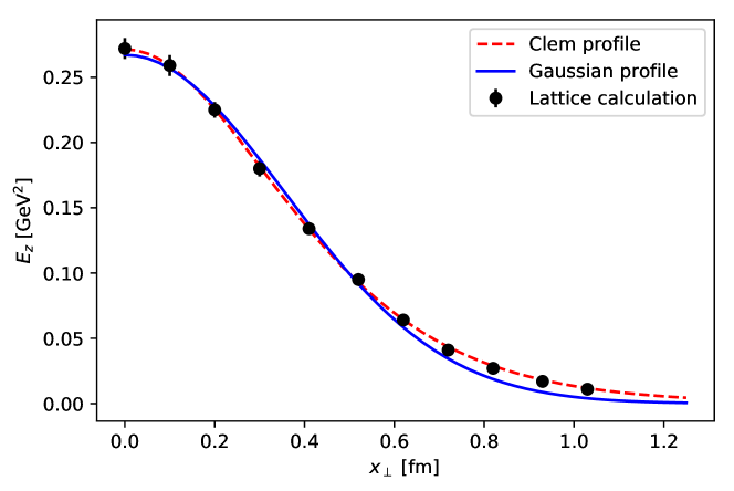
Figure 1: Profile of the electric field from the lattice calculation in ref. [55] compared to the fit by Clem [62] and a Gaussian distribution.

3 The Lund string hadronization

In the Lund string hadronization model, described in ref. [66], it is assumed that the dynamics of a single flux tube, and its breakup via quark pair production, is insensitive to the width of the tube. It is then approximated by an infinitely thin “massless relativistic string”. Essential features of the Lund hadronization model are first $q\bar{q}$ pair production via the Schwinger mechanism, and secondly the interpretation of gluons as transverse excitations on the string. This last assumption implies that the hadronization model is infrared safe and insensitive to the addition of extra soft or collinear gluons.

i) Breakup of a straight string

We here first describe the breakup of a straight flux tube or string between a quark and an antiquark. For simplicity we limit ourself to the situation with a single hadron species, neglecting also transverse momenta. For a straight string stretched between a quark and an anti-quark, the breakup to a state with $n$ hadrons is in the model given by the expression:

$$d\mathcal{P}\propto\prod_{i=1}^{n}\left[Nd^{2}p_{i}\delta(p^{2}_{i}-m^{2})\right]\delta^{(2)}\!\left(\sum p_{i}-P_{\mathrm{tot}}\right)\exp\left(-bA\right).$$ (7)

Here $p_{i}$ and $P_{\mathrm{tot}}$ are two-dimensional vectors. The expression is a product of a phase space factor, where the parameter $N$ expresses the ratio between the phase space for $n$ and $n-1$ particles, and the exponent of the imaginary part of the string action, $bA$. Here $b$ is a parameter and $A$ the space–time area covered by the string before breakup (in units of the string tension $\kappa$). This decay law can be implemented as an iterative process, where each successive hadron takes a fraction $z$ of the remaining light-cone momentum ($p^{\pm}=E\pm p_{z}$) along the positive or negative light-cone respectively. The values of these momentum fractions are then given by the distribution

$$f(z)=N\frac{(1-z)^{a}}{z}\exp(-bm^{2}/z).$$ (8)

Here $a$ is related to the parameters $N$ and $b$ in eq. (7) by normalization. (In practice $a$ and $b$ are determined from experiments, and $N$ is then determined by the normalization constraint.)

In applications it is also necessary to account for different quark and hadron species, and for quark transverse momenta. The result using Schwinger’s formalism for electron production in a homogenous electric field gives an extra factor $\exp(-\pi(\mu^{2}+p_{\perp}^{2})/\kappa)$, where $\mu$ and $p_{\perp}$ are the mass and transverse momentum for the quark and anti-quark in the produced pair. For details see e.g. ref. [66].

The result in eq. (8) is in principle valid for strings stretched between partons produced in a single space–time point, and moving apart as illustrated in the space–time diagram in fig. 2.

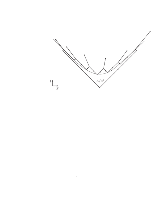
Figure 2: Breakup of a string between a quark and an anti-quark in a $x-t$ diagram. New $q\bar{q}$ pairs are produced around a hyperbola, and combine to the outgoing hadrons. The original $q$ and $\bar{q}$ move along light-like trajectories. The area enclosed by the quark lines is the coherence area $A$ in eq. (7), in units of the string tension $\kappa$. The notion of the ”hadronization time” is not well defined. It could be the time when the new $q\bar{q}$ pairs are produced, or when they meet for the first time to form a hadron (or something in between).

The expression in eq. (7) is boost invariant, and the hadrons are produced around a hyperbola in space–time. A Lorentz boost in the $x$-direction will expand the figure in the $(t+x)$ direction and compress it in the $(t-x)$ direction (or vice versa). Thus the breakups will be lying along the same hyperbola, and low momentum particles in a specific frame will always be the first to be produced in that special frame.

The typical proper time for the breakup points is given by

$$\langle\tau^{2}\rangle=\frac{1+a}{b\kappa^{2}}.$$ (9)

This does, however, not necessarily correspond to the ”hadronization time”, which might also be defined as the time when a quark and an anti-quark meet for the first time to form a hadron.

With parameters $a$ and $b$ determined by tuning to data from $e^{+}e^{-}$ annihilation at LEP, and $\kappa$ equal to 0.9-1 GeV/fm, eq. (9) gives a typical breakup time 1.5 fm, while the average time for the hadron formation is 2 fm. The typical hadronization time can therefore be estimated to 1.5-2 fm. This is important to keep in mind, as this value sets an upper limit on the time available for strings to interact.

ii) Hadronization of gluons

An essential component in Lund hadronization is the treatment of gluons. Here it is assumed that the width of the flux tube can be neglected, and that its dynamics can be approximated by an infinitely thin “massless relativistic string”. A quark at the endpoint of the string, carrying energy and momentum, moves along a straight line, affected by a constant force given by the string tension $\kappa$, reducing (or increasing) its momentum. A gluon is treated as a “kink” on the string, carrying energy and momentum and also moving along a straight line with the speed of light. A gluon carries both colour and anti-colour, and the string can be stretched from a quark, via a set of colour-ordered gluons, to an anti-quark (or alternatively as a closed gluon loop). Thus a gluon is pulled by two string pieces, and retarded by the force $2\kappa$. When it has lost its energy, the momentum-carrying kink is split in two corners, which move with the speed of light but carry no momentum.

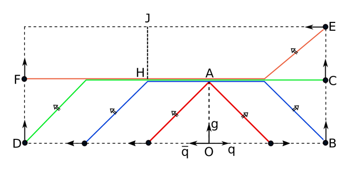
Figure 3: A $q-g-\bar{q}$ system moving out from a single point $O$ with energies 2, 2, and 3 units of energy respectively. The position of the string is shown at four consecutive times, marked by red, blue, green, and purple colour respectively.

A simple example is shown in figure 3. It shows a quark, a gluon, and an anti-quark moving out from a single point, called $O$ in the figure. They move outwards at right angles with energies 2, 2, and 3 units respectively. After 1 unit of time (equal to $\kappa^{-1}$ energy units) the gluon has arrived at point $A$ and lost all its energy. The gluon is then replaced by two corners connected by a straight section. The quark has lost its energy in point $B$. In the rest frame of the attached string piece it now turns back, gaining momentum in the opposite direction. In the figure frame it is turning $90^{\circ}$, and after meeting the string corner at $C$, it is instead pulled back and loosing energy. The anti-quark turns around in a similar way at point $D$. If the string does not break up in hadrons, the string evolution will be reversed. The kinks meet at point $H$, and the whole system collapses to a point $J$. (Note that this system is not in its rest frame.)

We note that although the string pieces initially move with a transverse velocity $1/\sqrt{2}$, after some time most of the string is at rest (the horizontal string pieces in figure 3. A soft gluon will soon stop and be replaced by a straight section stretched as if it were pulled out between the quark and the anti-quark. This implies that the string hadronization model is infrared safe; a soft gluon will only cause a minor modification on the string motion. The same is also true for a collinear gluon [66]. For a string with several gluons there will also be several new straight string pieces, which become more and more aligned with the directions of the endpoints, as described in ref. [68]. Therefore a string stretched over many rapidity units, and with several soft gluon kinks, will be pulled out in a way much more aligned with the beam axis, before it breaks into hadrons.

4 The string shoving picture

In the following we will describe the details in our new implementation of the string shoving model. First we recap the main idea as applied to two straight parallel string pieces, then we consider the interaction between two arbitrary string pieces, and describe a special Lorentz frame in which the shoving can be properly formulated. Finally we describe how we discretize the shoving into small fixed-size nudges and how these are ordered in time and applied to the final state hadrons.

4.1 Force between two straight and parallel strings

The force between two straight and parallel strings was discussed in ref. [30], We here shortly reproduce the treatment presented there. Just after the production of a string stretched between a quark and an anti-quark, the colour field is necessarily compressed, not only longitudinally but also transversely. They then expand transversely with the speed of light until they reach the equilibrium radius $R_{S}\sim$ 0.5-1 fm.

As illustrated in figure 1, the electric field $E$ obtained in lattice calculations, and fitted to the Clem formula, eq. (6), is also well approximated by a Gaussian

$$E=N\exp(-\rho^{2}/2R^{2}).$$ (10)

The normalization factor $N$ can be determined if the energy in the field (per unit length), given by $\int d^{2}\rho\,E^{2}/2$, is adjusted to a fraction $g$ of the string tension $\kappa$. This gives $N^{2}=2g\kappa/(\pi R^{2})$. As discussed in section 2.3, the simple bag model would give $g=1/2$. Due to the uncertainties in determining the properties of the flux tube, we will treat $R$ and $g$ as tunable parameters.

When the colour-electric fields in two nearby parallel strings overlap, the energy per unit length is given by $\int d^{2}\rho\,(\mathbf{E}_{1}+\mathbf{E}_{2})^{2}/2$. For a transverse separation $d_{\perp}$ this gives the interaction energy $2\kappa g\exp(-d_{\perp}^{2}/(4R^{2}))$. Taking the derivative with respect to $d_{\perp}$ then gives the force per unit length

$$f(d_{\perp})=\frac{g\kappa d_{\perp}}{R^{2}}\exp\left(-\frac{d_{\perp}^{2}}{4R^{2}}\right).$$ (11)

For a boost invariant system it is convenient to introduce hyperbolic coordinates

$$\tau=\sqrt{t^{2}-z^{2}},\,\,\,\,\,\eta_{st}=\ln((t+z)/\tau).$$ (12)

Near $z=0$ we get $\delta z=t\,\delta\eta_{st}$, and the force in eq. (11) gives $dp_{\perp}/dt\,\delta z=f(d_{\perp})$. Boost invariance then gives the two equations

$$\frac{dp_{\perp}}{\tau d\tau\,d\eta_{st}}=f(d_{\perp}),\,\,\,\,\frac{d^{2}d_{\perp}}{d\tau^{2}}=\frac{f(d_{\perp})}{\kappa}.$$ (13)

We have here assumed that the flux tubes are oriented in the same direction, leading to a repulsion. We have also argued in terms of an Abelian field, which means that if the fields are oppositely oriented there would be an attenuation of the fields rather than a repulsion. Since QCD is non-Abelian, the picture is slightly more complex, but the calculations are still valid. In case of two triplet fields in opposite directions, we get with probability 8/9 an octet field, which also leads to a repulsion when compressed. Only with probability 1/9 we get a singlet field, and in this case the strings are assumed to be removed through “colour reconnection”, as described in ref. [31]. Also for strings in other colour multiplets the string-string interaction is dominantly repulsive. This is not in conflict with the Abelian approximation, as discussed in section 2.3. A $q\bar{q}$ string is a colour singlet, where the quark is a coherent mixture of red, blue, and green (with corresponding anti-colours for the anti-quark). Similarly the endpoint of an octet string has a coherent combination of the 8 different colour charges.

4.2 String motion and the parallel frame

For a string piece between two (massless) partons, the motion and expansion of the sting is very simple in the rest frame of the two partons. If the partons have momenta along the $x$-axis, the position of the string ends are simply $x_{\pm}(t)=(t;\pm t,0,0)$, where we note that the ends move by the speed of light irrespective of the momentum of the partons.

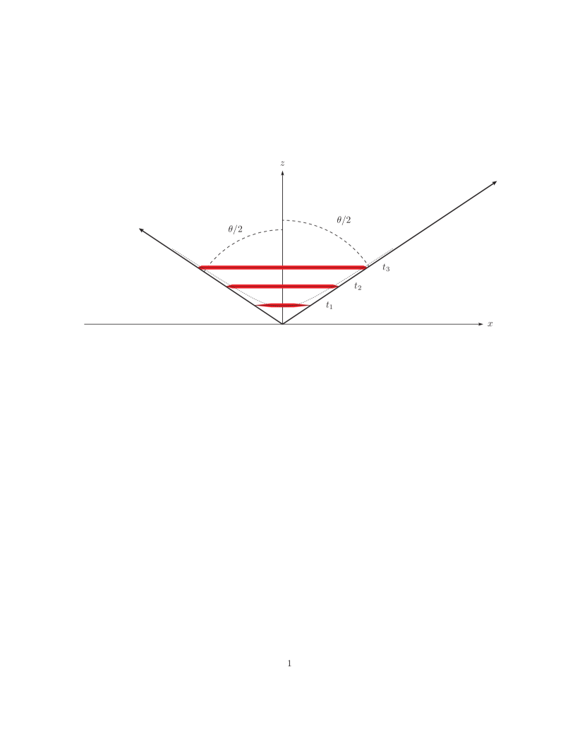
Figure 4: The time-evolution of a string piece between two partons in an arbitrary Lorentz frame. The system is rotated so that the momenta (the magnitude of which are indicated by the lengths of the arrows) of the of the partons are in the $x-z$ plane with equal but opposite angle w.r.t. the $z$-axis. The horizontal lines indicate the extension of the string horizontally and transversely at different times steps. The dotted curve indicates the hyperbola where in $x$ the proper time of the sting piece is equal to $R_{S}$ for a given $z=t\cos\frac{\theta}{2}$.

If we instead go to an arbitrary Lorentz frame we can also obtain a simple picture by rotating the partons so that they lie in the $x-z$ plane with the same but opposite angle $\theta/2$ with the $z$-axis, as shown in figure 4. Here the string ends still move by the speed of light and the position of string ends are given by $x_{\pm}(t)=(t;\,\pm t\sin\frac{\theta}{2},\,0,\,t\cos\frac{\theta}{2})$. A straight relativistic string is boost invariant and has no longitudinal momentum (similar to a homogeneous electric field). The energy and transverse momentum are given by $dE/dz=\kappa/\sqrt{1-v^{2}}$ and $dp_{\perp}/dz=v_{\perp}\,dE/dz$. The string in figure 4 is therefore still a straight line; it is just boosted transversely with velocity $v=\cos(\theta/2)$.

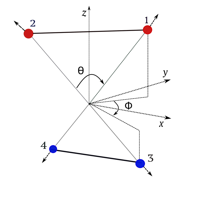
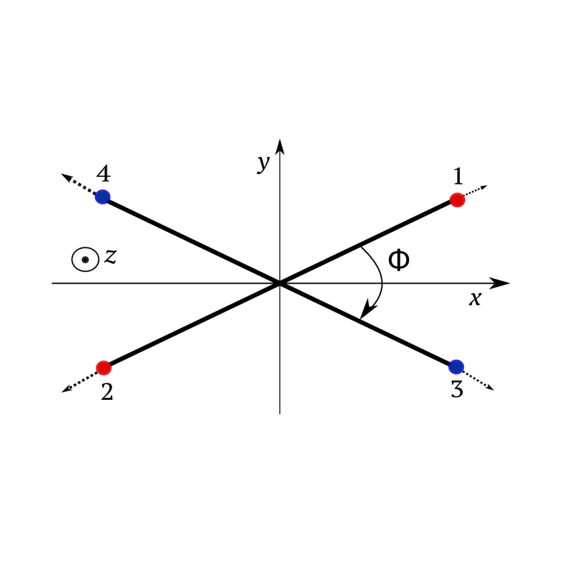
Figure 5: Schematic diagrams of two strings in their parallel frame. On the left, $\theta$ is the opening angle between the partons constituting each string, while on the right we show the skewness angle, $\phi$ in the projection on the $x-y$-plane of the two string pieces.

If we now want to study the interaction between two arbitrary string pieces, it is not possible to find a Lorentz frame where both these are always parallel to the $x$-axis, but it turns out that it is possible to find a frame where both always lie in parallel planes, perpendicular to the $z$-axis. To see this, we first we rotate the string piece in figure 4 an angle $\phi/2$ around the $z$-axis. Then we want another string piece with angle $\pi-\theta/2$ w.r.t. the the $z$-axis but rotated an angle $-\phi/2$. We then have the situation shown in figure 5 where the four partons have momenta (using pseudorapidity instead of the polar angle, to simplify the notation)

$$p_{1} = p_{\perp 1}\left(\cosh\frac{\eta}{2};\phantom{-}\cos\frac{\phi}{2},\phantom{-}\sin\frac{\phi}{2},\phantom{-}\sinh\frac{\eta}{2}\right),$$

$$p_{2} = p_{\perp 2}\left(\cosh\frac{\eta}{2};-\cos\frac{\phi}{2},-\sin\frac{\phi}{2},\phantom{-}\sinh\frac{\eta}{2}\right),$$

$$p_{3} = p_{\perp 3}\left(\cosh\frac{\eta}{2};\phantom{-}\cos\frac{\phi}{2},-\sin\frac{\phi}{2},-\sinh\frac{\eta}{2}\right),$$

$$p_{4} = p_{\perp 4}\left(\cosh\frac{\eta}{2};-\cos\frac{\phi}{2},\phantom{-}\sin\frac{\phi}{2},-\sinh\frac{\eta}{2}\right).$$ (14)

Here we have six unknown quantities and, for four massless momenta we can construct six independent invariant masses, $s_{ij}$. This means that for any set of four massless particles we can (as long as no two momenta are completely parallel) solve for the transverse momenta

$$p^{2}_{\perp 1}=\frac{s_{12}}{4}\sqrt{\frac{s_{13}s_{14}}{s_{23}s_{24}}},\,\,\,p^{2}_{\perp 2}=\frac{s_{12}}{4}\sqrt{\frac{s_{23}s_{24}}{s_{13}s_{14}}},\,\,\,p^{2}_{\perp 3}=\frac{s_{34}}{4}\sqrt{\frac{s_{13}s_{23}}{s_{14}s_{24}}},\,\,\,p^{2}_{\perp 4}=\frac{s_{34}}{4}\sqrt{\frac{s_{14}s_{24}}{s_{13}s_{23}}},$$ (15)

and the angles

$$\cosh\eta = \frac{s_{13}}{4p_{\perp 1}p_{\perp 3}}+\frac{s_{14}}{4p_{\perp 1}p_{\perp 4}},$$ (16)

$$\cos\phi = \frac{s_{14}}{4p_{\perp 1}p_{\perp 4}}-\frac{s_{13}}{4p_{\perp 1}p_{\perp 3}}.$$ (17)

We note that there is a mirror ambiguity in the solution, but apart from that we can now construct a Lorentz transformation to take any pair of string pieces to the desired frame, which we will call their parallel frame.

The sketches in figure 5 show the case where the four partons are produced in the same space–time point, which in general is not the case. The partons from the shower and MPI-machinery in PYTHIA8 are all assigned a space–time positions $(0;bx,by,0)$ in the lab frame assuming the standard picture that at t = 0 they are packed together at z = 0 and only with transverse separation. When a pair of string pieces are Lorentz transformed into their parallel frame, we assume that their respective production points are a simple average of the positions of the parton ends, giving us a $p^{a}_{0}=(t^{a}_{0};x^{a}_{0},y^{a}_{0},z^{a}_{0})$ for the string piece moving along the $z$-axis and the corresponding $p^{b}$ for the piece going in the other direction. From this we get for any given time, $t$, in the parallel frame that the string piece travelling along the $z$-axis has the length, $2(t-t^{a}_{0})\sin\frac{\theta}{2}$, and lies in a plane transverse to the $z$-axis. The string piece travelling in the opposite $z$ direction will similarly have a length $2(t-t^{b}_{0})\sin\frac{\theta}{2}$, which may be different, but the string will still always lie in a plane perpendicular to the $z$-axis. The endpoints of the two strings as a function of time then become

$$\!\!p^{a\pm}(t)\!\! = \!\!\!\left(t;\,x^{a}_{0}\pm(t-t_{0}^{a})\sin\frac{\theta}{2}\cos\frac{\phi}{2},\,y^{a}_{0}\pm(t-t_{0}^{a})\sin\frac{\theta}{2}\sin\frac{\phi}{2},\,z^{a}_{0}+(t-t_{0}^{a})\cos\frac{\theta}{2}\right)$$

$$\!\!p^{b\pm}(t)\!\! = \!\!\!\left(t;\,x^{b}_{0}\pm(t-t_{0}^{b})\sin\frac{\theta}{2}\cos\frac{\phi}{2},\,y^{b}_{0}\mp(t-t_{0}^{b})\sin\frac{\theta}{2}\sin\frac{\phi}{2},\,z^{b}_{0}-(t-t_{0}^{b})\cos\frac{\theta}{2}\right)$$ (18)

We see now that the distance between the two planes will change linearly with time as $\Delta_{z}(t)=z_{0}^{a}-z_{0}^{b}-t_{0}^{a}+t_{0}^{b}+2t\cos\frac{\theta}{2}$.

Besides the string motion we are also interested in the radius of the string. As indicated in figure 4 this radius is not constant along the string, but depends on the proper time of a point on the string. As the partons are assumed massless, the endpoints of the string always have zero proper time and the colour field there has not had time to spread out transversely. Looking at a point on the $x$-axis, $\bar{x}$, we can easily find the proper time

$$\tau(t,\bar{x})=\sqrt{(t-t_{0})^{2}\sin^{2}\frac{\theta}{2}-(\bar{x}-x_{0})^{2}-\left((\bar{x}-x_{0})\tan\frac{\phi}{2}-y_{0}\right)^{2}}.$$ (19)

The radius of the string will then vary linearly with $\tau$, from zero in the ends until it reaches the final equilibrium radius, $R_{S}=\tau_{S}\lesssim 1$ fm. After this the string’s width is fixed (as is indicated in figure 4) until it ultimately brakes, which on the average happens at $\tau_{H}\lesssim 2$ fm. In our implementation we have chosen to only allow the shoving to take place between string pieces at points in the parallel frame where both strings have proper times between $\tau_{S}$ and $\tau_{H}$.

Clearly there may also be shoving between string pieces where they have not yet reached their maximum radius, $R_{S}$. From the derivation of eq. (11) we see that the force will be larger and the range will be smaller. In our current implementation it is possible to set $\tau_{S}<R_{S}$ to allow for shoving also in these region, but the force is still given for $R=R_{S}$ in eq. (11). This can therefore only give an indication of the effect, and we have to postpone a quantified study to a later publication.

The shoving naturally stops when the string breaks, but there is a grey-zone after the string breaks and before the hadrons are fully formed where one could imagine that the string pieces in the hadrons being formed will still repel each other. Also, after the hadrons are fully formed we expect final state interactions between them. In this article we will not investigate final-state hadron interactions, although it is able to produce a sizable flow signal in $\mathrm{PbPb}$ collisions with Angantyr initial conditions [69], and has recently been implemented in P YTHIA 8 [70]. As indicated by the discussion about the inherent ambiguity in defining a “hadronization time” in section 3, defining a transition between a string-dominated final state at early times, and a hadron dominated final state at late times, will require scrutiny.

Another mechanism that reduces the shoving is when the endpoints have limited momenta, $k_{x}$ in the $x$-direction in the parallel frame. A parton loses momentum to the string at a rate $t\kappa$, and a gluon being connected to two string pieces loses momentum at twice that rate. After a time $t=|k_{x}|/2\kappa$ a gluon will therefore have lost all its momentum to the string and turn back, gaining momentum from the string in the opposite direction. As explained in section 3 (figure 3), this means that a new string region opens up which is then not in the same parallel $x-y$ plane. In this article we do not treat this new string region, but will comment on them in the following sections.

4.3 Generating the shoving

We now want to take the force between two string pieces in eq. (11) and apply it in the parallel frame. In ref. [30] everything was done in the laboratory frame and all strings were assumed to be parallel to the beam, and there generation of the shove was done by discretizing time and rapidity, calculating a tiny transverse momentum exchange in each such point. Here we instead use the parallel frame and discretize the transverse momentum into tiny fixed-size nudges.

Going back to the case where we have two completely parallel strings we have from the expression for the force from eq. (11) as

$$\frac{dp_{\perp}}{dtdx}=f(d_{\perp}(t))$$ (20)

and we get the total transverse momentum push on the strings as

$$\Delta p_{\perp}=\int dt\int dxf(d_{\perp}(t)),$$ (21)

where we note that the integration limits in $x$ are time-dependent. Now we will instead nudge several times with a fixed (small) transverse momentum, $\delta p_{\perp}$ according to some (unnormalized) probability distribution $P(t)$, which would give us the total push

$$\Delta p_{\perp}=\int dtP(t)\delta p_{\perp},$$ (22)

and for small enough $\delta p_{\perp}$ we can make the trivial identification

$$P(t)=\frac{1}{\delta p_{\perp}}\int dxf(d_{\perp}).$$ (23)

In any string scenario we can now order the nudges in time (in the parallel frame), and we can ask the question which of the pairs of string pieces will generate a transverse nudge of size $\delta p_{\perp}$ first. This gives us a situation that looks much like the one in parton showers where the question is which parton radiates first. And just as in a parton shower we will use the so-called Sudakov-veto algorithm [2, 71]. The main observation here is that the probability of nothing to happen before some time $t$ exponentiates, so that the (now normalized) probability for the first thing to happen at time $t$ is given by

$$P(t)e^{-\int_{t_{\min}}^{t}dt^{\prime}P(t^{\prime})}.$$ (24)

In the Sudakov-veto algorithm, one can then generate the next thing to happen in all pairs of strings individually, and then pick the pair where something happens first. In addition, since $P(t)$ may be a complicated function, one may chose to generate according to an simplified overestimate, $\hat{P}(t)\geq P(t)$, for which generating according to eq. (24) is easier. In this way we get a trial time, $t_{t}$, for the first thing to happen and then for that particular time calculate the true value of $P(t_{t})$, and accept the chosen time with a probability $P(t_{t})/\hat{P}(t_{t})$. If we reject, we then know we have underestimated the probability of nothing haven happened before $t_{t}$, which means we can generate the next trial time from $t_{\min}=t_{t}$ (in eq. (24)).

In our case we will make the overestimate by treating the strings as being completely parallel, only separated in $z$ and overestimating the limits in the $x$-integration. We then generate a time and a point along the $x$ axis, calculate the actual repulsion force there, to get the true probability for accepting the generated time.

The whole procedure can be seen as discretizing in time with a dynamically sized time step with larger time steps where the force is small, and vise versa. This is a very efficient way of evolving in time, and efficiency is important since we will calculate several nudges in each pair of string pieces in an event, and in the case of $AA$, there may be up to $\mathcal{O}(10^{4})$ string pieces per event at the LHC.

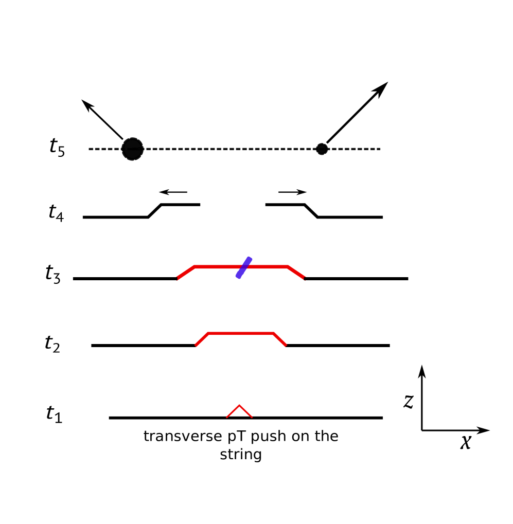
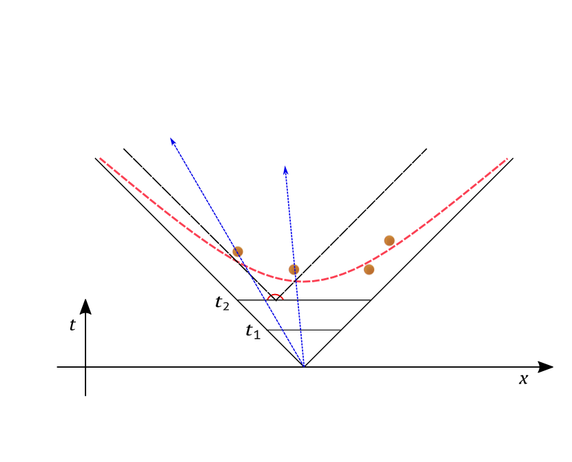
Figure 6: The left figure illustrates how a nudge deforms the geometry of a string piece from the time it is applied until the string breaks. The right figure illustrates how the final state hadrons that are will share the transverse momentum of a nudge are chosen.

4.4 Transferring the nudges to the hadons

Each time a nudge has been included somewhere along a string piece, the string is deformed slightly. It will correspond to a gluon kink on the string, however, since the transverse momentum of this kink is small, the $\delta p_{\perp}$ will soon start propagating along the string as indicated in figure 6 (left). A hadron that is produced along the string where there happens to be such a kink will absorb the corresponding nudge in transverse momentum. In practice this is done by finding the point where the proper time of the kink is $\tau_{H}$, the averaged hadronization time, and finding the primary hadron with the corresponding pseudorapidity (which is strongly correlated to the hyperbolic angle of the creation point, c.f. section 2.1) in the parallel frame, as sketched out in figure 6 (right). In this way each nudge is added to two hadrons from each of the two interacting string pieces. It should be noted that the fact that the two hadrons receive an extra transverse momentum in the same direction, will also mean that they come closer together in pseudorapidity. In addition, energy and momentum conservation is achieved by the adjusting the longitudinal momentum of the two hadrons separately in the two string pieces will also (on average) pull the hadrons closer together in rapidity. In the results below in section 6.2 this becomes visible in the overall multiplicity distribution.

It should be noted that the deformation of the string must be taken into account, not only in the pair of string pieces where the nudge was generated, but in all pairs involving one of the string pieces, triggering a recalculation of the next nudge in all these pairs. To do this in detail turns out to be forbiddingly time consuming, so instead we estimate an average shift of a string piece only after a certain number of nudges (typically $\mathcal{O}(10)$) and distribute it evenly along the string.

5 Results for simple initial state geometries

The most widely employed models for describing the space–time evolution of a final state interactions of heavy ion collisions as a QGP (after the decay of a CGC as discussed in the introduction), are based on relativistic dissipative fluid dynamics (see e.g. ref. [72] for a review). A key feature of such models, is that the observed momentum-space anisotropy of the final state, originates from the azimuthal spatial anisotropy of the initial state density profile. The final state anisotropy is quantified in flow coefficients ($v_{n}$’s), which are coefficients of the Fourier expansion of the single particle azimuthal particle yield, with respect to the event plane ($\Psi_{n}$) [73, 74]:

$$E\frac{d^{3}N}{d^{3}p}=\frac{1}{2\pi}\frac{d^{2}N}{p_{\perp}dp_{\perp}dy}\left(1+2\sum_{n=1}^{\infty}v_{n}\cos(n(\phi-\Psi_{n}))\right).$$ (25)

Here $E$ is the particle energy, $p_{\perp}$ the transverse momentum, $\phi$ the azimuthal angle and $y$ the rapidity. In this section, we will explore the models’ response to initial state geometry in a toy setup without non-flow contributions from jets, i.e. not real events, and thus we do not adapt the experimental calculation procedures involving $Q$-vectors (see section 6 where we compare to real data), but rather use the definition of the event plane angle from final state particles:

$$\Psi_{n}=\frac{1}{n}\arctan\left(\frac{\langle p_{\perp}\sin(n\phi)\rangle}{\langle p_{\perp}\cos(n\phi)\rangle}\right).$$ (26)

Flow coefficients can then be calculated using only final state information as:

$$v_{n}=\langle\cos(n(\phi-\Psi_{n}))\rangle.$$ (27)

“Toy” systems with known, simple input geometries are therefore better suited for exploring the basic model dynamics. In section 5.1 we set up a toy model for high energy nuclear–nuclear collisions in which the shoving model can be applied, and in section 5.2 we use the toy model to study the high-density behaviour of the shoving model. The parameters of the shoving model are not tuned, but set at reasonable values of $g=0.5$, $R_{S}=\tau_{S}=1$ fm amd $\tau_{H}=2$ fm.

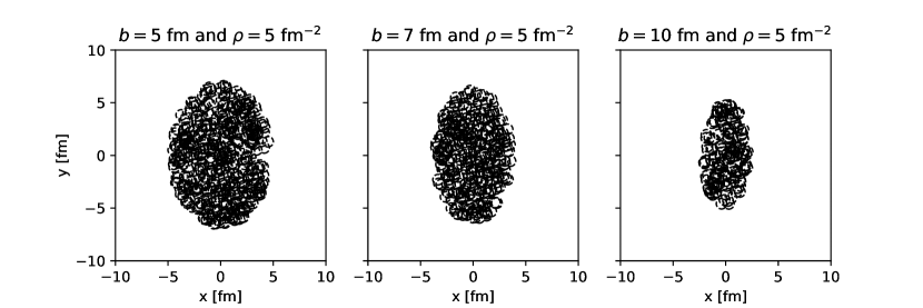
Figure 7: Examples of a sampled ellipse configuration in the Pb-Pb toy model, at three different impact parameters, with $\rho=5$ fm^-2.

5.1 Isolating flow effects to $v_{2}$ in a toy model

In this and the following section, we restrict our study to systems with constrained straight strings. The strings are drawn between $\mathrm{u}\bar{\mathrm{u}}$ pairs, with cms energy of 15 GeV, a small Gaussian kick in $p_{x}$, $p_{y}$, and $p_{z}$ fixed by energy-momentum conservation. This ensures that all strings will be stretched far enough in rapidity, that a study of final state hadrons with $|\eta|<1$ will not be perturbed by any edge effects. Final state hadrons studied in the figures, are all hadrons emerging from strings breakings (i.e. no decays enabled).

To study the model response in a heavy-ion like geometry, we set up a toy geometry in the shape of an ellipse, drawn between two overlapping nuclei of $r_{\mathrm{Pb}}=7.1$ fm. The ellipse has a minor axis ($\beta$) given by $2\beta=2r_{\mathrm{Pb}}-b$, and a major axis ($\alpha$) given by $2\alpha=\sqrt{4r^{2}_{\mathrm{Pb}}-b^{2}}$, where $b$ is the impact parameter. The elliptic overlap region is filled randomly with strings, given a certain density ($\rho$). Example events for $\rho=5\mathrm{~{}fm}^{-2}$ are shown in figure 7. We note that this configuration is deliberately chosen to maximize $v_{2}$ (elliptical flow) at the expense of $v_{3}$ (triangular flow), though with a fluctuating initial state geometry, some $v_{3}$ will always be present in order to study the response of the shoving model with minimal fluctuations.

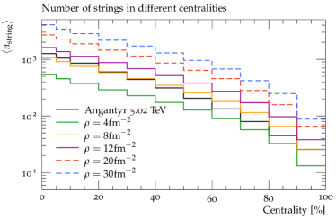
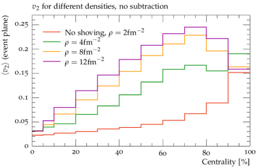
Figure 8: The number of string pieces (left) and $v_{2}$ (right) as function of centrality in the Pb-Pb toy model, for different values of $\rho$. In (right) compared to the number of strings generated by Angantyr at $\eta=0$ for Pb-Pb collisions at $\sqrt{s_{\mathrm{NN}}}=5.02$ TeV.

The initial anisotropy is given by the usual definition of the participant eccentricity [77], here employed on the strings:

$$\epsilon_{n}=\frac{\sqrt{\langle r^{2}\cos(n\phi)\rangle^{2}+\langle r^{2}\sin(n\phi)\rangle^{2}}}{\langle r^{2}\rangle},$$ (28)

where $r$ and $\phi$ are the usual polar coordinates of the string centers, but with the origin shifted to the center of the distribution. It is possible to calculate higher order moments of eq. (28), but here we will be concerned only with $\epsilon^{2}_{2}\{2\}=\langle\epsilon^{2}_{2}\rangle$, denoted by the short-hand $\epsilon_{2}$. We begin by studying average quantities as a function of collision centrality, here defined by the impact parameter of the two colliding nuclei, for exemplary

values of string density $\rho=\{4,8,12,20,30\}$ fm^-2. In figure 8 (left) we show the average number of strings in bins of centrality. The numbers are compared to the number of strings at $\eta=0$ generated by the Angantyr model [33] in Pb-Pb collisions at $\sqrt{s_{\mathrm{NN}}}=5.02$ TeV. The Angantyr model has been shown to give a good description of charged multiplicity at mid-rapidity in $AA$ collisions [78], and this comparison is therefore useful to provide a comparison to realistic string densities at current LHC energies.

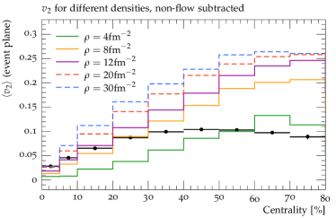
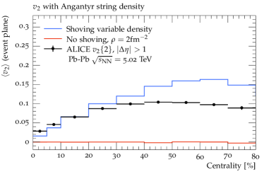
Figure 9: The $v_{2}$ flow coefficient with non-flow effects subtracted according to eq. (29) for different constant densities (left), and with string densities from Angantyr (right). Data from ALICE [79] added to guide the eye.

In figure 8 (b), the average $v_{2}$ as a function of centrality is shown for the same densities as figure 8 (a), as well as for a reference without shoving, with $\rho=2$ fm^-2. Again, several observations can be made. First of all, for a fixed centrality $v_{2}$ will increase with increasing density. Secondly, the non-flow contribution is rather large – in particular for peripheral centralities. This was also noted in our recent paper on the Angantyr model [33] using full Pb-Pb calculations. Third, for low string densities, the non-flow contribution is so large, that it takes over in peripheral events, meaning that the curve exhibits no turn-over at a characteristic centrality. Due to the toy nature of this setup, this cannot be taken as a firm prediction of the model, but should be investigated further in full simulations.

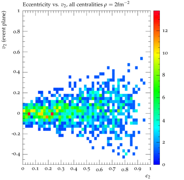
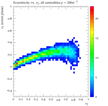
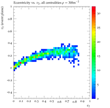
Figure 10: The correlation between $\epsilon_{2}$ and $v_{2}$ (non-flow subtracted) for four different densities, $\rho=2$ fm^-2 (upper left), $\rho=12$ fm^-2 (upper right), $\rho=20$ fm^-2 (lower left) and $\rho=30$ fm^-2 (lower right).

Since the goal of this section is to study the response to the elliptic geometry, the non-flow contribution will in the following be subtracted. To obtain this, each event is hadronized twice: once with shoving enabled, and once with shoving disabled. For each of the two final states, $\Psi_{n}$ and $\cos(n(\phi-\Psi_{n}))$ is calculated, and the final, non-flow subtracted, (inclusive) flow coefficients are given by:

$$v_{n}^{\mathrm{sub}}=\langle\cos(n(\phi-\Psi_{n}))_{\mathrm{shoving}}-\cos(n(\phi-\Psi_{n}))_{\mathrm{no~{}shoving}}\rangle_{\mathrm{all~{}events}}.$$ (29)

The flow coefficient $v_{2}$, with non-flow subtracted, is shown in figure 9. In the left part of the figure, $v_{2}$ is shown for different constant densities. The higher density samples now all have a characteristic turn-over at some centrality. It should be noted that the density intervals are not evenly spaced. Looking at $v_{2}$ in figure 9, the growth in the peak value decreases with higher density, like a saturation effect. Since final state multiplicity is proportional to the number of strings, the result in figure 9 suggests that the shoving model dynamically predicts a steep rise in the peak value of $v_{2}$ at low densities (corresponding to low energies, with otherwise fixed geometry), which should then slow down. The fact that string density is different at different centralities (as also shown in figure 8 (a)), is used to construct figure 9 (b). In this figure, string multiplicity for each toy-event are generated with Angantyr, and an elliptic initial condition of the same impact parameter is constructed. This provides more realistic string densities at different centralities, and as it can be seen, this construction does a reasonable job at describing $v_{2}$ as a function of centrality. A no-shoving reference is also added to this figure, and as expected, it is consistent with zero. Finally it can be added, both $v_{3}$ and $v_{4}$ are, as could be expected from the engineered initial conditions, both compatible with zero after the subtraction, indicating that non-flow has been successfully removed. (Not shown in any figure here.)

5.2 Towards the hydrodynamical limit at high string density

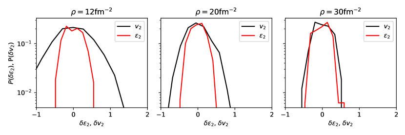
Figure 11: Probability distributions of $\epsilon_{2}$ and $v_{2}$ (non-flow subtracted) in the 20-30% centrality bin, for three different values of $\rho$.

As mentioned earlier, hydrodynamic calculations are often employed for heavy ion phenomenology, when it concerns interactions of the final state, leading to collective flow. Whether or not the shoving model will, in the end, describe heavy ion data to a satisfactory degree, it is interesting to ask to what kind of hydrodynamics the shoving model will become in the thermodynamic limit. While analytic exploration of this question will be left to future studies, it is possible at this point to study similarities in the phenomenology of the two approaches. An obvious route is to follow the paper by Niemi et al.[80], which studied the correlation between flow coefficients and eccentricities, and noted that $v_{2}$ and $v_{3}$ have a strong linear correlation with $\epsilon_{2}$ and $\epsilon_{3}$. In figure 10, we show the correlation between $\epsilon_{2}$ (from eq. (28)) and $v_{2}$, for four values of $\rho$. No centrality selection is performed, as the toy geometry of the system impose a strict relationship between eccentricity and centrality defined by impact parameter, and binning in centrality would thus not add any information. In the very dilute limit, $\rho=2$ fm^-2, in figure 10 (upper left), it is seen that even though $\langle v_{2}\rangle$ in figure 9 is non-zero, there is no strong correlation with $\epsilon_{2}$, and the distribution of $v_{2}$ is rather wide. At intermediate densities $\rho=12$ and $20$ fm^-2, in figure 10 (upper right) and (lower left), the strong correlation appears, though not as narrow as in ref. [80]. Finally for the densest considered state, $\rho=30$ fm^-2 in figure 10 (lower right) the correlation is, on average, similar to the more dilute ones, but more narrow.

To further study the scaling of $v_{2}$ with $\epsilon_{2}$, we study the scaled event-by-event variables:

$$\delta\epsilon_{2}=\frac{\epsilon_{2}-\langle\epsilon_{2}\rangle}{\langle\epsilon_{2}\rangle}\mathrm{,~{}~{}~{}and~{}~{}~{}}\delta v_{2}=\frac{v_{2}-\langle v_{2}\rangle}{\langle v_{2}\rangle}.$$ (30)

In figure 11 the distributions of $\delta\epsilon_{2}$ and $\delta v_{2}$, are shown for the densities $\rho=\{12,20,30\}$ fm^-2, in the 20-30% centrality bin. It should be noted that, due to the purely elliptical sampling region, the shape of the distribution cannot be compared directly to those of ref. [80]. The main conclusion is, however, clear. In the dense limit, in the rightmost panel, the two distributions are almost identical. This means that the shoving model, in this limit, reproduces a key global feature of hydrodynamics, namely full scaling of final state (purely momentum space) quantities with the global initial state geometry.

A notable discussion pertains to the issue whether or not heavy ion collisions at RHIC and LHC energies, reach a high enough string density for the shoving model to behave like hydrodynamics, as indicated above. In figure 8 (left), it was shown that Pb-Pb collisions at LHC energies produce an amount of strings corresponding to toy model densities of around 10 fm^-2 for very central events, 8 fm^-2 for mid-central events (corresponding to the two leftmost panels of figure 11) and less than 4 fm^-2 for the most peripheral events. Even though the toy model predicts scaling of $\langle v_{2}\rangle$ with $\langle\epsilon_{2}\rangle$, the fluctuations do not exhibit the same scaling. A further direct study of flow fluctuations in non-central heavy ion collisions would thus be of interest both on the phenomenological and experimental side.

6 Results with Angantyr initial states

In the previous section, we have shown that given a simple initial state of long, straight strings without any soft gluons, the shoving mechanism can produce a response which (a) scales with initial state geometry in the same way as a hydrodynamic response, and (b) can produce flow coefficients in momentum space at the same level as measured in experiments. In this section we go a step further, and present the response of the model given a more realistic initial string configuration, as produced by the Angantyr model, which can be compared to data. In section section 4 we described several of the challenges faced when interfacing the shoving model to an initial state containing many soft gluons, which in particular is the case in $AA$ collisions. Throughout this section we use the same canonical values of shoving model parameters as in the previous section.

6.1 Results in $\mathrm{pp}$ collisions

Already the original implementation of the shoving model was shown in ref. [30] to give a satisfactory description of the $\mathrm{pp}$ “ridge”. We will in this section focus on flow observables as calculated at high energy heavy ion experiments, i.e. flow coefficients calculated using the generic framework formalism [81, 82], in the implementation in the Rivet program [83].

It is in principle possible to generate $\mathrm{pp}$ events using the normal P YTHIA MPI model [84, 85, 86]. It would, however, be computationally inefficient, since emphasis should be given to high multiplicity results. The results presented here therefore use the modifications of the MPI framework presented as part of the Angantyr heavy ion model [33], notably the ability to bias the impact parameter selection towards very central pp collisions, and re-weighting back to the normal distribution.

We first note, that while the shoving mechanism does not change the total multiplicity of an event, it will change the multiplicity in fiducial region measured by an experiment, because it will push particles from the unmeasured low-$p_{\perp}$ region to (measured) higher $p_{\perp}$. It is therefore necessary to slightly re-tune the model parameters, to obtain a correct description of basic observables such as $p_{\perp}$ distributions and total multiplicity. In practise, the parameter $p_{\perp,0}$, which regulates the $2\rightarrow 2$ parton cross section is increased from the default value of 2.28 to 2.4. In figure 12 we show a comparison between P YTHIA (with the above mentioned impact parameter sampling) and P YTHIA + shoving, for a few standard minimum-bias observables, compared the charged $p_{\perp}$ distribution (left), the distribution of number of charged particles (middle) and $\langle p_{\perp}\rangle(N_{ch})$ (right), all at $\sqrt{s}=13$ TeV. Data by ATLAS [87], the analysis implemented in the Rivet framework [88].

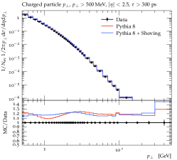
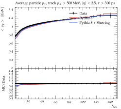
Figure 12: Comparison of P YTHIA (non-diffractive) to P YTHIA + shoving to basic $p_{\perp}$ (left), multiplicity (middle) and $\langle p_{\perp}\rangle$ distributions in $\mathrm{pp}$ collisions at $\sqrt{s}=13$ TeV to data by ATLAS.

The agreement between simulation and data for the multiplicity distribution, is not as good as normally expected from P YTHIA . This is expected, as only non-diffractive collisions were simulated. More interesting is the slight difference between the two simulations, where it is clearly visible that in spite of the re-tuning, shoving still produce more particles in the high-$N_{ch}$ limit. In the $p_{\perp}$ distribution, it is seen that shoving has the effect of increasing the spectrum around around $p_{\perp}=1$ GeV. While the normalization if off (due to the exclusion of diffractive events in the simulation), shoving brings the shape of the low-$p_{\perp}$ part of the spectrum closer to data. Finally the $\langle p_{\perp}\rangle(N_{ch})$ is almost unchanged.

We now turn our attention to flow coefficients, and show $v_{2}$ calculated by two-particle correlations in figure 13. In figure 13 (left) the multiplicity dependence of $v_{2}\{2\}$ with $|\Delta\eta|>1.4$ is shown, and in figure 13 (right) the $p_{\perp}$-dependence of $v_{2}\{2\}$ ($|\Delta\eta|>2$) in high multiplicity events is shown. Several conclusions can be drawn from the two figures.

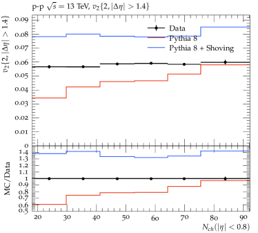
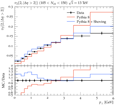
Figure 13: Comparison to $v_{2}\{2\}$ as function of multiplicity with ALICE high multiplicity trigger (left), and versus $p_{\perp}$ in high multiplicity events (right). Data from $\mathrm{pp}$ collisions at $\sqrt{s}=13$ TeV by ALICE [89] and CMS [90].

First of all, it is seen that $v_{2}$ as a function of multiplicity (in figure 13 (left)) is too high with shoving enabled. We emphasize that the model parameters have not been tuned to reproduce this data, and in particular that successful description of this data will also require a good model for the spatial distribution of strings in a $\mathrm{pp}$ collision – a point we will return to in a moment. We do, however, note that the additional $v_{2}$ added by the shoving model, persists even with an $\eta$ separation of correlated particles (as $|\Delta\eta|$ cuts are applied), a feature which separates the shoving model from e.g. colour reconnection approaches, which have been pointed out to produce flow-like effects in $\mathrm{pp}$ collisions [91, 92, 93]. We also note that the $p_{\perp}$-dependence of $v_{2}$ is drastically improved, as seen in figure 13 (right). In particular the high-$p_{\perp}$ behaviour of this quantity is interesting, as it decreases wrt. the baseline when shoving is enabled.

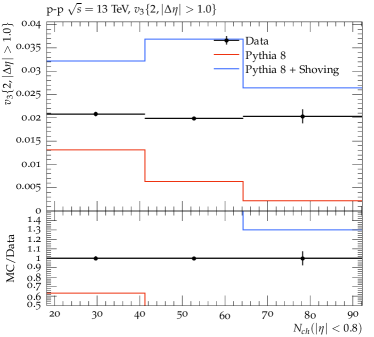
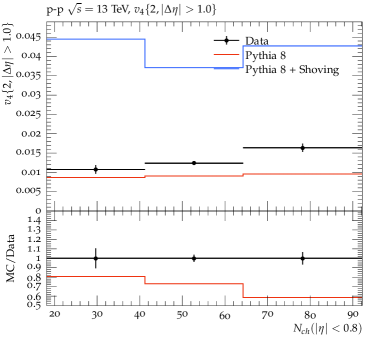
Figure 14: Comparison to $v_{3}\{2\}$ (left) and $v_{4}\{2\}$ (right) as function of multiplicity with ALICE high multiplicity trigger. Data from $\mathrm{pp}$ collisions at $\sqrt{s}=13$ TeV by ALICE [89].

In figure 14 comparisons to $v_{3}\{2\}$ (left) and $v_{4}\{2\}$ (right) are performed. While it is clear that shoving adds a sizeable contribution to both, it is equally clear that data is not very well reproduced. We remind the reader that any $v_{n}$ produced by the shoving model comes about as a response to the initial geometry, and the initial geometry used by default in P YTHIA , consists of two overlapping 2D Gaussian distributions. It was shown in ref. [94], that applying more realistic initial conditions, can drastically change the eccentricities of the initial state in $\mathrm{pp}$ collisions. So while the description at this point is not perfect, the observations that a clear effect is present, bears promise for future studies. Further on, correlations between flow coefficients, the so-called symmetric cumulants [82, 95], will be an obvious step. But at this point, without satisfactory description of the $v_{n}$’s themselves, it is not fruitful to go on to even more advanced observables.

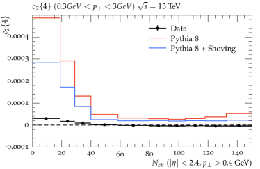
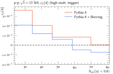
Figure 15: The four-particle cumulant $c_{2}\{4\}$, compared to data from CMS [90] (left), and with the ALICE high multiplicity trigger (no data, right).

Finally, in figure 15, we show results for the four-particle cumulant $c_{2}\{4\}$. We briefly remind the reader about some definitions. The 2- and 4-particle correlations in a single event are given by the moments [81]:

$$\langle 2\rangle = \langle\sum_{i,j}\exp[in(\phi_{i}-\phi_{j})]\rangle$$

$$\langle 4\rangle = \langle\sum_{i,j,k,l}\exp[in(\phi_{i}+\phi_{j}-\phi_{k}-\phi_{l})]\rangle.$$ (31)

The averages are here taken over all combinations of 2 or 4 non-equal particles in one event. The four particle cumulant is the all-event averaged 4-particle azimuthal correlations, with the 2-particle contribution subtracted:

$$c_{n}\{4\}=\langle\langle 4\rangle\rangle-2\langle\langle 2\rangle\rangle^{2}.$$ (32)

The double average here means first an average over particles in one event, and then average over all events.

As discussed in ref. [96], when the correlation is dominated by flow and the multiplicity is high, then the flow coefficient $v_{2}\{4\}$ is given by $\sqrt[4]{-c_{2}\{4\}}$. Clearly $c_{2}\{4\}$ must be negative for this to be realized. This, in turn, means that the relative difference between the 2 -and 4-particle azimuthal correlations, must be right from eq. (32). As it was also pointed out in ref. [96], the non-flow contribution to four-particle correlations is much smaller than for two-particle correlations, as the cumulant becomes flow-dominated when $v_{n}\gg 1/M^{3/4}$ ($M$ is the multiplicity) in the former case, but only when $v_{n}\gg 1/\sqrt{M}$ in the latter. In a $\mathrm{pp}$ collision $M$ is small compared to a heavy ion collision, and it can therefore be reasonably expected that the four particle correlations will only be flow dominated at sufficiently high multiplicity. Since data show a real $v_{2}\{4\}$, the importance of the sign of $c_{2}\{4\}$ in model calculations for $\mathrm{pp}$, have recently been highlighted [97, 98]. Importantly, standard hydrodynamic treatments do not obtain a negative sign of $c_{2}\{4\}$ in $\mathrm{pp}$ collisions, even with specifically engineered initial conditions [99].

In the results from the shoving model in figure 15, we note that while a negative $c_{2}\{4\}$ is not produced when comparing to CMS results, it is produced in high multiplicity events in the ALICE acceptance, using the high multiplicity trigger. There are several possible reasons for this apparent discrepancy. The acceptances are quite different, and since the sign of $c_{2}\{4\}$ is an observed characteristic, rather than a fundamental feature of the model, it is difficult to point out why a given model should produce different results in different acceptances – though it is possible. More interesting, is the possible effect of the high multiplicity trigger. In figure 15 (left), it is seen that both default P YTHIA , as well as P YTHIA with the shoving model, over-predicts $c_{2}\{4\}$ at low-multiplicity by a large margin. As noted in the original paper, this is also the case for the 2-particle cumulant. A reasonable explanation for this over-prediction could be, that P YTHIA collects too many particles in mini-jets in general. With a high multiplicity forward trigger, a strong bias against this effect is put in place, and the underlying model behaves more reasonable. In any case, the finding of a negative $c_{2}\{4\}$ in high-multiplicity events with the shoving model is an interesting and non-trivial result, which will be followed up in a future study.

6.2 Results in Pb-Pb collisions

We now turn to Pb-Pb collisions, where we use the Angantyr model in PYTHIA keeping the same settings as in section 6.1. The results for Pb-Pb collision events at 5.02 TeV has been compared to ALICE data points via Rivet routines. The anisotropic flow coefficients plotted here have been calculated, as in the previous section, using multi-particle cumulant methods as done in the ALICE experiment.

Centrality measures used in these analyses are of two kinds: for the plot in figure 16 we use the centrality binning of the generated impact parameter by Angantyr, and for the plots in figure 17, we use Angantyr generated centrality binning which mimics the experimental centrality definition where in ALICE the binning is in the integrated signal in their forward and backward scintillators. However, the difference between the two centrality measures is small in Pb-Pb collisions [83].

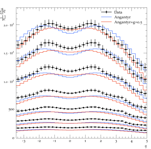
Figure 16: Charged particle multiplicity over a wide range of $\eta$ in Pb-Pb collisions at $\sqrt{s_{NN}}=5.02$ TeV for centralities 0-5%, 5-10%, 10-20%, …, 50-60% [100].

In figure 16, we plot the charged particle multiplicity for seven centrality classes (0-5%, 5-10%, 10-20%, 20-30%, 30-40%, 40-50%, 50-60%) as a function of pseudorapidity in the range $-3.5<\eta<5$ for $\sqrt{s_{NN}}=5.02$ TeV in Pb-Pb collisions comparing it to the study performed by ALICE[100]. We use this figure as our control plot to check that when we turn shoving on, the description of other observables are not destroyed.

We observe that this implementation fairly well preserves the Angantyr description of the multiplicity distributions. The overall multiplicity of the shoving curve is however a bit lower when compared to default Angantyr, which is because of the increased pT0Ref as mentioned in 6.1. Also, as discussed in section 4.3, when strings are shoved and the particles on average get a larger $p_{\perp}$ which also means that they come closer together in pseudorapidity. The overall effect is that particles are generally dragged closer towards mid-rapidity, reducing the two-humped structure seen for plain Angantyr.

We will look into further improvement of the multiplicity description by shoving through tuning, normalization of the distribution functions and accurate description of centrality as in experiments in the future.

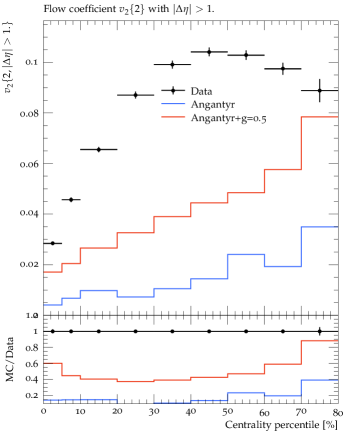
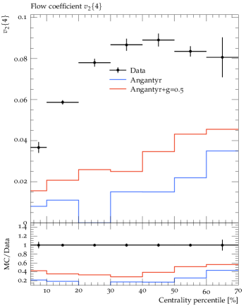
Figure 17: The flow coefficient $v_{2}\{2\}$(left) with $|\Delta\eta|>1$ and $v_{2}\{4\}$(right) for $0.2<p_{\perp}<5.0$ GeV in Pb-Pb collisions at $\sqrt{s_{\mathrm{NN}}}=5.02$ TeV[79].

Figure 17 presents the centrality dependence of the harmonic flow coefficient $v_{2}$ from two-particle cumulant on the left with $|\Delta\eta|>1$ and four-particle cumulants on the right, integrated over the $p_{\perp}$ range $0.2<p_{\perp}<5.0$ GeV for 5.02 TeV Pb-Pb collisions [79] for generated centrality. We note that Angantyr with shoving results in an increased $v_{2}$ in the right direction with respect to data. We see in data that $v_{2}\{2\}$ increases from central to peripheral collisions, reaching a maximum of around 0.10 between $40-50$% centrality. $v_{2}\{4\}$ also shows a similar behaviour with a maximum around 0.09 between $40-50$% centrality. String shoving result clearly lacks the curvature of the data points, but doubles the contribution in $v_{2}\{2\}$ as compared to Angantyr. The underlying cause for this behaviour is that the current implementation of shoving alone is not sufficient to generate the large overall response to the anisotropy in the initial collision geometry of the nuclei. An increased $g$ factor or delayed hadronization time or an early onset of shoving, and a combination of these factors, do not give rise to enough $v_{2}$ either.

In section 5.1, we showed that shoving can generate sufficient $v_{2}$ as seen in data with completely straight strings without any gluon kinks. With Angantyr, we have more realistic final states with many and often soft gluon emissions from the multi-parton interactions and the initial- and final-state evolution models, which hinder the process of strings shoving each other by cutting short their interaction time, hence resulting in the overall observation of the lack of enough transverse nudges generated via this mechanism.

7 Conclusions and outlook

In this paper we have argued that a hot thermalized plasma is not necessarily formed even in central $AA$ collisions, not even in Pb–Pb collisions at the highest attainable energies at the LHC. Instead we note that the string-based approach to simulating hadronic final states in the Angantyr model in P YTHIA 8 gives a very reasonable description of the number and general distribution of particles in $AA$ events, and take this as an incentive to study string hadronization in dense collision systems more carefully.

Our string picture is qualitatively different from the more conventional picture, where the colliding nuclei are described in terms of a CGC, that in the moment of collision turns into a so-called glasma, which very soon decays into a thermalized QGP. Similar to the string picture, the glasma has longitudinal fields stretched between the nucleus remnants, and these fields are kept together in flux tubes as the remnants move apart. There are, however, also essential differences. The glasma turns rapidly into a thermalized plasma. Such a plasma expands longitudinally in a boost invariant way, with decreasing energy density as a result. The initial density must therefore be quite high to give the observed particle density after freezeout. In contrast the energy density in the strings is constant up to the time for hadronization. When the strings become longer, the energy in the new string pieces is taken from the removing nucleus remnants, and not from depleting the energy in the strings already formed. In the string scenario we estimate the energy density at mid-rapidity to around 5 GeV/fm³ (in $\mathrm{PbPb}$ at the LHC), while in the glasma we find that it ought to be one or two orders of magnitude higher.

The low energy density in the string scenario implies that the vacuum condensate is very important to form the strings. The break-down of the glasma is often motivated by the so-called “Nielsen–Olesen instabilities”. These authors showed that a longitudinal chromo-electric field added to the QCD Fock vacuum is instable, and transverse fields grow exponentially. This growth does not go on forever. Instead higher order corrections will lead to a Higgs potential analogous to the potential describing the condensate of Cooper-pairs in a superconductor or the vacuum condensate in the EW Higgs model. Adding a (not too strong) linear field to this non-trivial ground state will then give flux tubes, similar to the vortex lines in a superconductor. We take this as an indication that it may indeed be possible that strings can be formed and actually survive the initial phase of the collision, without a thermalized plasma being formed. (The energy density needed in the glasma may, however, be strong enough to destroy the ”superconducting” phase.)

Another important difference between the two scenarios is that the glasma contains both chromo-electric and chromo-magnetic fields, not only chromo-electric fields as in the string picture. This implies CP-violating effects in the glasma, but this feature is not discussed in this paper.

In an earlier paper we argued that in a dense environment where the strings overlap in space–time, they should repel each other and we showed with a very simple model that this could induce flow in $\mathrm{pp}$. Here we have motivated the model further, and compared to lattice calculations to estimate the transverse shape and energy distribution of the string-like field. We have also improved the implementation of the model, where the strings no longer have to be completely parallel in order to calculate the force between them. Instead we show that for a pair of arbitrary string pieces, we can always find a Lorentz frame where they will be stretched out in parallel planes, allowing us to easily calculate the force there. We have further improved the time discretization, and instead of processing string interactions in fixed time intervals, the shoving model is implemented as a parton shower with dynamical time steps, greatly improving the computational performance of the model. Finally we have improved the procedure for transferring the nudges from string interactions to final state hadrons.

The implementation used for obtaining the results presented here is not yet quite complete. Although it circumvents the production of huge amounts of soft gluons in the shoving, which was a major problem for our previous implementation, it still has a problem with dealing with the soft gluons that are already there from the initial- and final-state parton showers. Gluon kinks loose energy with twice the force compared to a quark. A soft gluon therefore will soon loose all its energy, and new straight sections of the string will be formed, which in the current implementation are not taken into account.

In addition the implementation only allows shoving at points in space–time after the strings have expanded to the equilibrium size, $R_{S}\sim\tau_{S}$, and before they start to break up in hadrons at proper times around $\tau_{H}$. Clearly shoving should be present also at times before $\tau_{S}$, and the force between very close strings should then be higher, but our implementation currently cannot handle situations with varying string radii. Also, at times later than $\tau_{H}$, after the string break-up, one could expect some shoving between the hadrons being formed, and after they are formed one needs to consider final state re-scattering.

In light of these shortcomings of the current implementation, it is not surprising that when we apply the model to complete partonic final states generated by Angantyr, we cannot quantitatively reproduce the amount of $v_{2}$ measured in experiments. But we do see that the shoving actually does give rise to flow effects. We also see that in $\mathrm{pp}$ we currently get a bit too large $v_{2}$, but we would like to emphasise that we have here not tried to do any tuning of the model parameters. Instead these are kept at canonical values,

To investigate the model further and to make it plausible that the shoving model, when implemented in full, actually may be able to reproduce also quantitatively the flow effects measured in $AA$  collisions, we looked at what happens when applying it to a toy model of the initial state. To account for the missing string pieces due to soft gluons, we here used parallel strings without gluon kinks. The strings are randomly distributed with variable density in an ellipsoid shape in impact parameter space. In this way the shoving was unhampered by soft gluons, and we found that the model is able to get the azimuthal anisotropies in momentum space as expected from the eccentricity of the shape in impact parameter. By then matching the string density to the one we have in Angantyr for different centralities, we could also see that the resulting $v_{2}$ was much closer to measured data.

Showing that we can get reasonable azimuthal anisotropies in $AA$  collisions using a purely string-based scenario is, of course, not enough to prove that a thermalized QGP is not formed in such collisions. To do this we need to also be able to describe other measurements, such as strangeness enhancement and jet quenching and, more importantly find new observables where a string based scenario predicts results that cannot be reconciled with the QGP picture. And for this we not only need to improve the implementation of the shoving model, but also revisit our rope model and also our “swing” model for colour reconnections. The rope model has been shown to give reasonable descriptions of strangeness enhancement in high multiplicity $\mathrm{pp}$, and using the parallel frame presented here, we should be able to get a better handle on the space–time picture of the string overlaps needed to be able to apply it in $AA$. Also for the swing model we can take advantage of the parallel frame to properly understand which partons may reconnect and when and where they may do so. And since in the parallel frame hard and soft partons are treated on an equal footing this could also have interesting effect on jets.

In the end we hope that these models will be implemented in P YTHIA 8 together with the Angantyr model, so that we get a complete platform for generating fully hadronic final states that can be compared to any type of measurement in any kind of collision ($AA$, $\mathrm{p}A$, $\mathrm{pp}$, …). This would then give us a perfect laboratory to investigate a purely string-based picture as an alternative to the conventional QGP approach.

Appendix A Vortex lines in a superconductor

The microscopic properties in a superconductor, the magnetic field, $H$, and the condensate wavefunction (order parameter), $\psi$, can be determined by the LG equations (see e.g. ref. [52]). The theory contains two characteristic lengths, the penetration depth $\lambda$ for the magnetic field and the coherence length $\xi$ for the condensate. In its generalization to a relativistic theory, the Lagrangian contains a Higgs potential for the condensate. Here the lengths $\lambda$ and $\xi$ correspond to the (inverse) masses of the gauge boson and the Higgs particle respectively.

For a flux tube the wavefunction $\psi$ is undetermined along a “vortex line”, and has a phase changing by $2\pi n$ when going around the vortex line, with $n$ an integer. The total flux in the flux tube is then quantized to $n$ times a flux quantum $\Phi_{0}=2\pi/q$, where for a normal superconductor $q=2e$ is the charge of a Cooper pair. This quantum would also correspond to the charge of a magnetic monopole. The change in phase is related to a vortex-like current in the condensate, which keeps the flux confined within the flux tube.

At the boundary between a normal and a superconducting phase, the pressure from the condensate and the magnetic field balance each other. The condensate goes to zero over a distance $\xi$ in the superconductor, and the magnetic field is suppressed over a distance $\lambda$. As a result, when $\xi$ is larger than $\lambda$ (or more exactly $\xi>\sqrt{2}\,\lambda$), both the condensate and the field are suppressed over a range $\xi-\lambda$. This is a type I superconductor, and it implies that the surface provides a positive contribution to the energy. In equilibrium the surface then tends to be as small as possible. If in contrast $\lambda$ is larger than $\xi$ (type II superconductor), the condensate and the field can coexist over a range $\sim\lambda-\xi$, and the surface provides a negative contribution to the energy, favouring a large surface. If the flux tube has more than one flux quantum, there is then a tendency to split it into a number of vortices, each with one unit of flux. In case of a large total flux, there is a repulsive force between nearby flux tubes. The system will then tend to expand, forming an “Abrikosov lattice”.

The interaction between the condensate and the electromagnetic field in a superconductor is described by the LG equations, which in its relativistic generalization corresponds to the Abelian Higgs model relevant for the Abelian projection of the QCD field. The Lagrange density is here given by

$$\mathcal{L}=-\frac{1}{4}F_{\mu\nu}F^{\mu\nu}+[(\partial_{\mu}+ieA_{\mu})\psi^{*}][(\partial_{\mu}-ieA_{\mu})\psi]-\alpha|\psi|^{2}-\frac{\beta}{2}|\psi|^{4}.$$ (33)

When the parameter $\alpha$ is smaller than zero, the scalar field $\psi$ forms a condensate $\psi=\psi_{0}=\sqrt{-\alpha/\beta}$. The mass of the Higgs particle and the massive gauge boson, given by $\sqrt{-2\alpha}$ and $e\sqrt{-2\alpha/\beta}$ respectively, correspond to (the inverse of) the coherence length $\xi$ and the penetration depth $\lambda$. The LG equations are obtained from Euler-Lagrange’s equations varying $\psi$ (or $\psi^{*}$) and $A_{\mu}$.

In an extreme type II superconductor with $\xi\ll\lambda$, the LG equations have a solution $\psi=const.\,\,e^{-i\phi}$ (for $\rho>\xi$), for a vortex line which carries one unit of flux. The corresponding magnetic field is here given by

$$H(\rho)=C\cdot K_{0}(\rho/\lambda),$$ (34)

where $C=\Phi/(2\pi\lambda^{2}$) is a constant, $\Phi$ is the total flux, and $K_{0}$ is a modified Bessel function. The Bessel function has a logarithmic dependence on $\rho$ for $\rho<\lambda$, but falls exponentially for $\rho>\lambda$. The field is confined within this range by an electric current $j=\lambda\,|\mathrm{curl}\,\mathbf{H}|=(C/\lambda)\,K_{1}(\rho/\lambda)$ (also valid for $\rho>\xi$). In this extreme case, when $\xi$ is very small, the contribution to the energy from destroying the condensate is also small, and the energy of the flux tube, the string tension $\kappa$, is given by the sum of the field energy and the energy in the current:

$$\kappa=\int_{\xi}d^{2}\!\rho\,\frac{1}{2}\left\{H(\rho)^{2}+\lambda^{2}(\mathrm{curl}\,\mathbf{H}(\rho))^{2}\right\}.$$ (35)

We note that the energy is dominated by the contribution from the current, where $K_{1}(\rho/\lambda)$ is singular and $\sim\lambda/\rho$ for small $\rho$. Thus the total energy is proportional to $\ln(\lambda/\xi)$ for very small $\xi$.

When $\xi$ is smaller than $\lambda$, but not close to zero, the following approximate solution is given by Clem [62]:

$$H(\rho)=C\,K_{0}(x_{\perp}/R),\,\,\,\,\,\mathrm{with}\,\,\,R=\sqrt{\rho^{2}+\xi^{2}_{v}}\,\,\,\,\mathrm{and}\,\,\,C=\Phi/(2\pi\lambda\,\xi_{v}\,K_{1}(\xi_{v}/\lambda)).$$ (36)

The new distance scale $\xi_{v}$ depends on the ratio $\kappa_{LG}\equiv\lambda/\xi$, and is close to $\xi$ for $\kappa_{LG}\approx 1/\sqrt{2}$, i.e. for a superconductor on the border between type I and type II. The expression in eq. (36) satisfies the one of the LG equations (obtained by varying the field $A_{\mu}$) and Ampèr’s equation $\mathbf{j}=\mathrm{curl}\,\mathbf{B}=\mathrm{curl}\,\mathrm{curl}\,\mathbf{A}$. It does, however, not satisfy the equation obtained by varying $\psi$, and for $\xi>\lambda$ this equation can be badly violated.

In a superconductor there are magnetic flux tubes, and magnetic monopoles would be confined. In QCD colour-electric flux tubes and colour-electric charges are confined. Thus for the Abelian projection the fields $F_{\mu\nu}$ will be replaced by the dual fields $\widetilde{F}_{\mu\nu}$, as discussed in section 2.2.

References

- [1] T. Sjöstrand, S. Ask, J. R. Christiansen, R. Corke, N. Desai, P. Ilten et al., An introduction to PYTHIA 8.2, Comput. Phys. Commun. 191 (2015) 159 [1410.3012].
- [2] T. Sjöstrand, S. Mrenna and P. Z. Skands, PYTHIA 6.4 Physics and Manual, JHEP 05 (2006) 026 [hep-ph/0603175].
- [3] J. Bellm et al., Herwig 7.0/Herwig++ 3.0 release note, Eur. Phys. J. C76 (2016) 196 [1512.01178].
- [4] M. Bähr et al., Herwig++ Physics and Manual, Eur. Phys. J. C 58 (2008) 639 [0803.0883].
- [5] Sherpa collaboration, E. Bothmann et al., Event Generation with Sherpa 2.2, SciPost Phys. 7 (2019) 034 [1905.09127].
- [6] T. Gleisberg, S. Höche, F. Krauss, M. Schönherr, S. Schumann, F. Siegert et al., Event generation with SHERPA 1.1, JHEP 02 (2009) 007 [0811.4622].
- [7] E. Gotsman, E. Levin and U. Maor, A comprehensive model of soft interactions in the LHC era, Int. J. Mod. Phys. A 30 (2015) 1542005 [1403.4531].
- [8] V. Khoze, A. Martin and M. Ryskin, Elastic scattering and Diffractive dissociation in the light of LHC data, Int. J. Mod. Phys. A 30 (2015) 1542004 [1402.2778].
- [9] S. Ostapchenko, Monte Carlo treatment of hadronic interactions in enhanced Pomeron scheme: I. QGSJET-II model, Phys. Rev. D 83 (2011) 014018 [1010.1869].
- [10] W. Broniowski, M. Chojnacki, W. Florkowski and A. Kisiel, Uniform Description of Soft Observables in Heavy-Ion Collisions at s(NN)**(1/2) = 200 GeV**2, Phys. Rev. Lett. 101 (2008) 022301 [0801.4361].
- [11] B. Schenke, S. Jeon and C. Gale, Elliptic and triangular flow in event-by-event (3+1)D viscous hydrodynamics, Phys. Rev. Lett. 106 (2011) 042301 [1009.3244].
- [12] H. Song, S. A. Bass, U. Heinz, T. Hirano and C. Shen, Hadron spectra and elliptic flow for 200 A GeV Au+Au collisions from viscous hydrodynamics coupled to a Boltzmann cascade, Phys. Rev. C83 (2011) 054910 [1101.4638].
- [13] F. G. Gardim, F. Grassi, M. Luzum and J.-Y. Ollitrault, Anisotropic flow in event-by-event ideal hydrodynamic simulations of GeV Au+Au collisions, Phys. Rev. Lett. 109 (2012) 202302 [1203.2882].
- [14] C. Gale, S. Jeon, B. Schenke, P. Tribedy and R. Venugopalan, Event-by-event anisotropic flow in heavy-ion collisions from combined Yang-Mills and viscous fluid dynamics, Phys. Rev. Lett. 110 (2013) 012302 [1209.6330].
- [15] J. Noronha-Hostler, M. Luzum and J.-Y. Ollitrault, Hydrodynamic predictions for 5.02 TeV Pb-Pb collisions, Phys. Rev. C93 (2016) 034912 [1511.06289].
- [16] A. Andronic, P. Braun-Munzinger, K. Redlich and J. Stachel, Decoding the phase structure of QCD via particle production at high energy, Nature 561 (2018) 321 [1710.09425].
- [17] A. Kovner, L. D. McLerran and H. Weigert, Gluon production from nonAbelian Weizsacker-Williams fields in nucleus-nucleus collisions, Phys. Rev. D 52 (1995) 6231 [hep-ph/9502289].
- [18] A. Kovner, L. D. McLerran and H. Weigert, Gluon production at high transverse momentum in the McLerran-Venugopalan model of nuclear structure functions, Phys. Rev. D 52 (1995) 3809 [hep-ph/9505320].
- [19] T. Lappi and L. McLerran, Some features of the glasma, Nucl. Phys. A772 (2006) 200 [hep-ph/0602189].
- [20] R. Venugopalan, From Glasma to Quark Gluon Plasma in heavy ion collisions, J. Phys. G35 (2008) 104003 [0806.1356].
- [21] F. Gelis, Color Glass Condensate and Glasma, Int. J. Mod. Phys. A28 (2013) 1330001 [1211.3327].
- [22] D. Kharzeev, R. Pisarski and M. H. Tytgat, Possibility of spontaneous parity violation in hot QCD, Phys. Rev. Lett. 81 (1998) 512 [hep-ph/9804221].
- [23] D. Kharzeev, A. Krasnitz and R. Venugopalan, Anomalous chirality fluctuations in the initial stage of heavy ion collisions and parity odd bubbles, Phys. Lett. B 545 (2002) 298 [hep-ph/0109253].
- [24] G. Chen, R. J. Fries, J. I. Kapusta and Y. Li, Early Time Dynamics of Gluon Fields in High Energy Nuclear Collisions, Phys. Rev. C 92 (2015) 064912 [1507.03524].
- [25] N. Nielsen and P. Olesen, An Unstable Yang-Mills Field Mode, Nucl. Phys. B 144 (1978) 376.
- [26] N. Nielsen and P. Olesen, Electric Vortex Lines From the Yang-Mills Theory, Phys. Lett. B 79 (1978) 304.
- [27] E. S. Weibel, Spontaneously Growing Transverse Waves in a Plasma Due to an Anisotropic Velocity Distribution, Phys. Rev. Lett. 2 (1959) 83.
- [28] CMS collaboration, V. Khachatryan et al., Observation of Long-Range Near-Side Angular Correlations in Proton-Proton Collisions at the LHC, JHEP 09 (2010) 091 [1009.4122].
- [29] ALICE collaboration, J. Adam et al., Enhanced production of multi-strange hadrons in high-multiplicity proton-proton collisions, Nature Phys. 13 (2017) 535 [1606.07424].
- [30] C. Bierlich, G. Gustafson and L. Lönnblad, Collectivity without plasma in hadronic collisions, Phys. Lett. B 779 (2018) 58 [1710.09725].
- [31] C. Bierlich, G. Gustafson, L. Lönnblad and A. Tarasov, Effects of Overlapping Strings in pp Collisions, JHEP 03 (2015) 148 [1412.6259].
- [32] X.-N. Wang and M. Gyulassy, HIJING: A Monte Carlo model for multiple jet production in p p, p A and A A collisions, Phys. Rev. D44 (1991) 3501.
- [33] C. Bierlich, G. Gustafson, L. Lönnblad and H. Shah, The Angantyr model for Heavy-Ion Collisions in PYTHIA8, JHEP 10 (2018) 134 [1806.10820].
- [34] E. Avsar, G. Gustafson and L. Lönnblad, Small-x dipole evolution beyond the large-N(c) imit, JHEP 01 (2007) 012 [hep-ph/0610157].
- [35] G. Gustafson, L. Lönnblad, A. Ster and T. Csörgő, Total, inelastic and (quasi-)elastic cross sections of high energy pA and ⋆ A reactions with the dipole formalism, JHEP 10 (2015) 022 [1506.09095].
- [36] J. Bjorken, Highly Relativistic Nucleus-Nucleus Collisions: The Central Rapidity Region, Phys. Rev. D 27 (1983) 140.
- [37] B. Andersson, G. Gustafson, J. Hakkinen, M. Ringner and P. Sutton, Is there screwiness at the end of the QCD cascades?, JHEP 09 (1998) 014 [hep-ph/9807541].
- [38] B. Schenke, P. Tribedy and R. Venugopalan, Fluctuating Glasma initial conditions and flow in heavy ion collisions, Phys. Rev. Lett. 108 (2012) 252301 [1202.6646].
- [39] BRAHMS collaboration, I. G. Bearden et al., Pseudorapidity distributions of charged particles from Au+Au collisions at the maximum RHIC energy, Phys. Rev. Lett. 88 (2002) 202301 [nucl-ex/0112001].
- [40] BRAHMS collaboration, A. Jipa, Overview of the results from the BRAHMS experiment, Acta Phys. Hung. A22 (2005) 121 [nucl-ex/0404011].
- [41] B. Schenke, P. Tribedy and R. Venugopalan, Event-by-event gluon multiplicity, energy density, and eccentricities in ultrarelativistic heavy-ion collisions, Phys. Rev. C 86 (2012) 034908 [1206.6805].
- [42] H. B. Nielsen and P. Olesen, A Quantum Liquid Model for the QCD Vacuum: Gauge and Rotational Invariance of Domained and Quantized Homogeneous Color Fields, Nucl. Phys. B 160 (1979) 380.
- [43] J. Ambjørn, N. Nielsen and P. Olesen, A Hidden Higgs Lagrangian in QCD, Nucl. Phys. B 152 (1979) 75.
- [44] P. Olesen, On the QCD Vacuum, Phys. Scripta 23 (1981) 1000.
- [45] G. ’t Hooft, A Property of Electric and Magnetic Flux in Nonabelian Gauge Theories, Nucl. Phys. B 153 (1979) 141.
- [46] M. Baker, J. S. Ball and F. Zachariasen, Dual QCD: A Review, Phys. Rept. 209 (1991) 73.
- [47] G. ’t Hooft, Topology of the Gauge Condition and New Confinement Phases in Nonabelian Gauge Theories, Nucl. Phys. B 190 (1981) 455.
- [48] J. Carmona, M. D’Elia, A. Di Giacomo, B. Lucini and G. Paffuti, Color confinement and dual superconductivity of the vacuum. 3., Phys. Rev. D 64 (2001) 114507 [hep-lat/0103005].
- [49] P. Cea and L. Cosmai, Abelian monopole and vortex condensation in lattice gauge theories, JHEP 11 (2001) 064 [hep-lat/0103019].
- [50] G. Ripka, Dual superconductor models of color confinement, vol. 639. 2004, 10.1007/b94800, [hep-ph/0310102].
- [51] A. Di Giacomo, QCD monopoles, abelian projections and gauge invariance, 1707.07896.
- [52] P. G. de Gennes, Superconductivity in Metals and Alloys. Addison–Wesley Publ. Co., 1966, 1989.
- [53] K. Johnson, The M.I.T. Bag Model, Acta Phys. Polon. B 6 (1975) 865.
- [54] K.-I. Kondo, S. Kato, A. Shibata and T. Shinohara, Quark confinement: Dual superconductor picture based on a non-Abelian Stokes theorem and reformulations of Yang–Mills theory, Phys. Rept. 579 (2015) 1 [1409.1599].
- [55] P. Cea, L. Cosmai, F. Cuteri and A. Papa, Flux tubes in the SU(3) vacuum: London penetration depth and coherence length, Phys. Rev. D89 (2014) 094505 [1404.1172].
- [56] M. Baker, P. Cea, V. Chelnokov, L. Cosmai, F. Cuteri and A. Papa, Isolating the confining color field in the SU(3) flux tube, Eur. Phys. J. C79 (2019) 478 [1810.07133].
- [57] M. Baker, P. Cea, V. Chelnokov, L. Cosmai, F. Cuteri and A. Papa, The confining color field in SU(3) gauge theory, Eur. Phys. J. C80 (2020) 514 [1912.04739].
- [58] S. Nishino, K.-I. Kondo, A. Shibata, T. Sasago and S. Kato, Type of dual superconductivity for the Yang–Mills theory, Eur. Phys. J. C79 (2019) 774 [1903.10488].
- [59] A. Shibata, K.-I. Kondo, S. Nishino, T. Sasago and S. Kato, Type of dual superconductivity for and Yang–Mills theories, 1903.10487.
- [60] A. Shibata, K.-I. Kondo, S. Kato and T. Shinohara, Non-Abelian dual superconductivity in SU(3) Yang-Mills theory: dual Meissner effect and type of the vacuum, Phys. Rev. D87 (2013) 054011 [1212.6512].
- [61] N. Battelli and C. Bonati, Color flux tubes in Yang-Mills theory: an investigation with the connected correlator, Phys. Rev. D99 (2019) 114501 [1903.10463].
- [62] J. R. Clem, J. Low Temp. Physics 18 (1975) 427.
- [63] R. Sommer, Scale setting in lattice QCD, PoS LATTICE2013 (2014) 015 [1401.3270].
- [64] R. G. Edwards, U. M. Heller and T. R. Klassen, Accurate scale determinations for the Wilson gauge action, Nucl. Phys. B517 (1998) 377 [hep-lat/9711003].
- [65] S. Necco and R. Sommer, The N(f) = 0 heavy quark potential from short to intermediate distances, Nucl. Phys. B622 (2002) 328 [hep-lat/0108008].
- [66] B. Andersson, G. Gustafson, G. Ingelman and T. Sjöstrand, Parton Fragmentation and String Dynamics, Phys. Rept. 97 (1983) 31.
- [67] X. Artru, Classical String Phenomenology. 1. How Strings Work, Phys. Rept. 97 (1983) 147.
- [68] T. Sjöstrand, Jet Fragmentation of Nearby Partons, Nucl. Phys. B248 (1984) 469.
- [69] A. V. da Silva, W. M. Serenone, D. Dobrigkeit Chinellato, J. Takahashi and C. Bierlich, Improved heavy-ion collision baseline based on perturbative QCD and hadronic rescattering, 2002.10236.
- [70] T. Sjöstrand and M. Utheim, A Framework for Hadronic Rescattering in pp Collisions, 2005.05658.
- [71] L. Lönnblad, Fooling Around with the Sudakov Veto Algorithm, Eur. Phys. J. C73 (2013) 2350 [1211.7204].
- [72] U. Heinz and R. Snellings, Collective flow and viscosity in relativistic heavy-ion collisions, Ann. Rev. Nucl. Part. Sci. 63 (2013) 123 [1301.2826].
- [73] S. Voloshin and Y. Zhang, Flow study in relativistic nuclear collisions by Fourier expansion of Azimuthal particle distributions, Z. Phys. C 70 (1996) 665 [hep-ph/9407282].
- [74] A. M. Poskanzer and S. Voloshin, Methods for analyzing anisotropic flow in relativistic nuclear collisions, Phys. Rev. C 58 (1998) 1671 [nucl-ex/9805001].
- [75] A. Badea, A. Baty, P. Chang, G. M. Innocenti, M. Maggi, C. Mcginn et al., Measurements of two-particle correlations in collisions at 91 GeV with ALEPH archived data, Phys. Rev. Lett. 123 (2019) 212002 [1906.00489].
- [76] Belle collaboration, A. Abdesselam et al., Measurement of two-particle correlations in hadronic collisions at Belle, 8, 2020, 2008.04187.
- [77] Z. Qiu and U. W. Heinz, Event-by-event shape and flow fluctuations of relativistic heavy-ion collision fireballs, Phys. Rev. C 84 (2011) 024911 [1104.0650].
- [78] ALICE collaboration, S. Acharya et al., Centrality and pseudorapidity dependence of the charged-particle multiplicity density in XeXe collisions at =5.44TeV, Phys. Lett. B 790 (2019) 35 [1805.04432].
- [79] ALICE collaboration, J. Adam et al., Anisotropic flow of charged particles in Pb-Pb collisions at TeV, Phys. Rev. Lett. 116 (2016) 132302 [1602.01119].
- [80] H. Niemi, G. Denicol, H. Holopainen and P. Huovinen, Event-by-event distributions of azimuthal asymmetries in ultrarelativistic heavy-ion collisions, Phys. Rev. C 87 (2013) 054901 [1212.1008].
- [81] A. Bilandzic, R. Snellings and S. Voloshin, Flow analysis with cumulants: Direct calculations, Phys. Rev. C 83 (2011) 044913 [1010.0233].
- [82] A. Bilandzic, C. H. Christensen, K. Gulbrandsen, A. Hansen and Y. Zhou, Generic framework for anisotropic flow analyses with multiparticle azimuthal correlations, Phys. Rev. C 89 (2014) 064904 [1312.3572].
- [83] C. Bierlich et al., Confronting experimental data with heavy-ion models: RIVET for heavy ions, Eur. Phys. J. C 80 (2020) 485 [2001.10737].
- [84] T. Sjöstrand and M. van Zijl, A Multiple Interaction Model for the Event Structure in Hadron Collisions, Phys. Rev. D36 (1987) 2019.
- [85] T. Sjöstrand and P. Z. Skands, Multiple interactions and the structure of beam remnants, JHEP 03 (2004) 053 [hep-ph/0402078].
- [86] R. Corke and T. Sjöstrand, Interleaved Parton Showers and Tuning Prospects, JHEP 03 (2011) 032 [1011.1759].
- [87] ATLAS collaboration, G. Aad et al., Charged-particle distributions in = 13 TeV pp interactions measured with the ATLAS detector at the LHC, Phys. Lett. B 758 (2016) 67 [1602.01633].
- [88] C. Bierlich et al., Robust Independent Validation of Experiment and Theory: Rivet version 3, SciPost Phys. 8 (2020) 026 [1912.05451].
- [89] ALICE collaboration, S. Acharya et al., Investigations of Anisotropic Flow Using Multiparticle Azimuthal Correlations in pp, p-Pb, Xe-Xe, and Pb-Pb Collisions at the LHC, Phys. Rev. Lett. 123 (2019) 142301 [1903.01790].
- [90] CMS collaboration, V. Khachatryan et al., Evidence for collectivity in pp collisions at the LHC, Phys. Lett. B 765 (2017) 193 [1606.06198].
- [91] A. Ortiz Velasquez, P. Christiansen, E. Cuautle Flores, I. Maldonado Cervantes and G. Paić, Color Reconnection and Flowlike Patterns in Collisions, Phys. Rev. Lett. 111 (2013) 042001 [1303.6326].
- [92] C. Bierlich and J. R. Christiansen, Effects of color reconnection on hadron flavor observables, Phys. Rev. D92 (2015) 094010 [1507.02091].
- [93] C. Bierlich, Microscopic collectivity: The ridge and strangeness enhancement from string-string interactions, Nucl. Phys. A 982 (2019) 499 [1807.05271].
- [94] C. Bierlich and C. O. Rasmussen, Dipole evolution: perspectives for collectivity and A collisions, JHEP 10 (2019) 026 [1907.12871].
- [95] J. L. Albacete, H. Petersen and A. Soto-Ontoso, Symmetric cumulants as a probe of the proton substructure at LHC energies, Phys. Lett. B778 (2018) 128 [1707.05592].
- [96] N. Borghini, P. M. Dinh and J.-Y. Ollitrault, Flow analysis from multiparticle azimuthal correlations, Phys. Rev. C64 (2001) 054901 [nucl-th/0105040].
- [97] W. Zhao, Y. Zhou, H. Xu, W. Deng and H. Song, Hydrodynamic collectivity in proton-proton collisions at 13 TeV, Phys. Lett. B 780 (2018) 495 [1801.00271].
- [98] J. Adolfsson et al., QCD Challenges from pp to A-A Collisions, 3, 2020, 2003.10997.
- [99] W. Zhao, Y. Zhou, K. Murase and H. Song, Searching for small droplets of hydrodynamic fluid in proton–proton collisions at the LHC, Eur. Phys. J. C 80 (2020) 846 [2001.06742].
- [100] ALICE collaboration, J. Adam et al., Centrality dependence of the pseudorapidity density distribution for charged particles in Pb-Pb collisions at TeV, Phys. Lett. B 772 (2017) 567 [1612.08966].