Encoder-decoder semantic segmentation models for electroluminescence images of thin-film photovoltaic modules

Abstract

We consider a series of image segmentation methods based on the deep neural networks in order to perform semantic segmentation of electroluminescence (EL) images of thin-film modules. We utilize the encoder-decoder deep neural network architecture. The framework is general such that it can easily be extended to other types of images (e.g. thermography) or solar cell technologies (e.g. crystalline silicon modules). The networks are trained and tested on a sample of images from a database with 6000 EL images of Copper Indium Gallium Diselenide (CIGS) thin film modules. We selected two types of features to extract, shunts and so called “droplets”. The latter feature is often observed in the set of images. Several models are tested using various combinations of encoder-decoder layers, and a procedure is proposed to select the best model. We show exemplary results with the best selected model. Furthermore, we applied the best model to the full set of 6000 images and demonstrate that the automated segmentation of EL images can reveal many subtle features which cannot be inferred from studying a small sample of images. We believe these features can contribute to process optimization and quality control.

Keywords: encoder-decoder neural networks, thin-film, electroluminescence imaging

I Introduction

Recently there has been an increasing interest in automated image analysis of spatially resolved characterization methods for Photo Voltaic (PV) modules such as electroluminescencetypo: luminescence (EL) [1, 2, 3, 4, 5, 6]. Such automated image analysis aims at quality control of modules and is thus of great interest for manufacturers, PV system owners, and insurance companies, as it allows for a systematic inspection of a large number of modules, both prior and after installation.

Several commonly used PV imaging methods exists which reveal detailed information on the state of a PV module. Examples include ultraviolet fluorescence luminescence (UVFL) to inspect the encapsulation of a module, Electro- and Photo-luminescence, which provides detailed information on the local electrical properties of the solar cells, and thermography, with which the operation temperature distribution within a module may be estimated.

These imaging methods may all be applied prior to installing the modules and after installation to inspect a system during operation. Thus, manufacturers may use these methods in production quality control. System owners and insurance companies may also use PV imaging methods to determine the cause of module performance issues or to support warranty claims and determine liabilities.

An automated image analysis allows the systematic analysis of a large number of module images. Thus, it can greatly contribute to classify degradation modes of modules and to the identification of early warning signs or degradation.

In this work we demonstrate the application of novel semantic image segmentation methods based on deep neural networks. The aim of an image segmentation is to assign a label to every pixel in an image. In our case we would like to identify pixels in EL images that correspond to some defect in a module.

We apply our segmentation models to a database of 6000 EL images of thin-film modules. Several common defect types are identified and different models are trained to detect these defect. Furthermore, we propose an approach to select the best models from the set of the obtained trained segmentation networks.

The main challenge that we have to overcome in this work comes from the type of our PV modules. Whereas for crystalline silicon there exists a well established catalogue of defects visible in EL images [7], such a catalogue does not exist for thin-film modulesthin-film defect catalogue. Therefore, our methods must be flexible enough to be easily adapted for different defects. This motivates the choice of the deep neural network methodology that we use.

We demonstrate that our approach reliably detects various defect types. Furthermore, a combined statistical evaluation of the EL image database reveals hidden features in EL images that are not observed in individual images of the modules. Our methods can be easily adapted for other types of defects, as well as other types of technology.

The paper is organized as follows. Section II reviews literature on the subject of automatic image analysis. The available data used in this study and its preprocessing is discussed in Section III. Section IV elaborates on our data and methodology. Section V discusses the results. Lastly, this work is concluded in Section VI.

II Related works

To review the relevant literature in a structured way we split this section into two subsections. Firstly, we review the research on the automatic visual inspection in photovoltaics. Secondly, we discuss works in other application fields, where approaches similar to this paper have been used. This allows us to overview methods used so far in photovoltaics community as well as to capture research trends in other image analysis fields.

One of such trends is the gradual replacement of feature-based methods by machine learning techniques. By a feature-based method, we understand here an approach that applies some transformation to an image that is tailored for extraction of some particular information. On the other hand, the machine learning methods usually solve some generic tasks such as regression or classification, which are then adapted to a particular application. This work also adapts a set of generic image segmentation methods based on deep neural networks.

II-A Image analysis in PV

In photovoltaics automated image analysis methods aim to solve different tasks. Although very different aims are pursued, there are some common methods applied. For this reason we briefly review related works on image analysis which can be roughly categorized as follows; detecting and locating defects and other structures of interest, forecasting module performance, and image collection itself.

Most work on locating and identifying structures of interest revolves around cracks in crystalline silicon solar modules. [8] [8], [9] [9, 10] used a pipeline consisting of an anisotropic diffusion and certain shape analysis algorithms to localise cracks in EL images.

[11] [11] consider image representation in the Fourier domain to identify position of cracks, breaks and finger interruptions. There the Fourier transformed image is filtered by setting high-frequency coefficients associated with lines artifacts to zero. Then the defects are identified by comparing the original image and the high-pass filtered image. Due to the assumptions on the shape of the defect, the method has difficulties detecting defects of more complex shapes.

[12] [12] introduce a supervised learning method for defect identification that uses Independent Component Analysis (ICA). Manually selected defect-free solar cell subimages are used to find a set of independent basis images with an independent component analysis (ICA), that are consequently used in a cosine distance to determine presence of a defect in a test sample image.

Some works focus on an automatic visual inspection of very specific parts of a PV module. [13] [13] proposed a machine vision algorithm to examine electrical contacts. Whereas [14] [14] describe a method for an automatic detection of finger interruptions via binary clustering.

Infrared imaging is mostly used to detect hot-spots. As IR imaging provides fairly direct information on the local surface temperature of a module, relatively simple image processing algorithms can be used. [15] [15] uses watershed transform algorithm to identify the hot-spots. [16] [16], and [17] [17] use clustering algorithms to segment IR image and identify hotspots. [18] developed a thresholding method for hot spot detection [18].

There are several research directions that have been established in order to build models that forecast electrical characteristics from images. [19] [19] uses a physical model to calculate the operating voltage of individual crystalline solar cells by EL imaging.

More recent works do not rely on a particular physical model and train a machine learning method to extract the required information from the data. [20] [20] proposed a system for forecasting power loss, localisation and type of soiling from RGB images of solar modules. Their approach uses deep neural network architectures similar to ones we use in this paper.

[3] [3] train an SVM classifier based on the extracted feature descriptors (SURF, KAZE, FAST), and a VGG-net based neural network in order to identify defective cells that have an impact on power reduction of the whole module.

[1] [1] proposes a Convolution Neural Network (CNN) architecture to forecast IV characteristics from a PL image as a production process control procedure.

When it comes to an application of these automatic methods to the real data, several practical problems arise. It is often the case that images taken in field conditions suffer from various distortions due to the position of a module in front of a camera, lens distortions, blurring due to wind and shocks. Such distortions introduce complications in automatic image processing. Therefore, a certain amount of work has been done in the direction of EL image preprocessing analysis methods [2, 5, 6].

The preprocessing steps are important for IR images as well. [21] [21] use the grey-level co-occurrence matrix to identify the location of the solar panels in IR images of the operating photovoltaic plants.

II-B Image analysis in other fields

Convolution neural networks are becoming a standard tool in automated image analysis. We provide here several references that use similar methods as used in this work.

[22] [22] developed a CNN architecture to detect cracks in steel. The proposed architecture is compared with a method that use hand-crafted feature description.

A neural network architecture has been proposed to identify cracks on the road, [23]. It has been demonstrated that the method outperforms methods based on SVM and Boosting.

[24] [24] use encoder-decoder neural networks to extract agriculture field boundaries from satellite images. [25] [25] use U-net with VGG11 encoder network to segment satellite images in the Inria Aerial Image Labelling Dataset [26].

Image segmentation is an important topic in medical image analysis as well. [27] [27] performs semantic segmentation of the brain tumours using MRI imaging. They explore the possibility to combine a simple CNN in a cascaded fashion. [28] [28] use deep neural network to classify different types of skin cancer. [29] [29] use combination of CNN and Recurrent Neural Networks (RNN) to identify a surgical tool location in medical imaging. [30] [30] adapt the U-net encoder-decoder style architecture for the 3-dimensional input signal of the MRI images.

III Data

The data was acquired within the framework of the PEARL-TF project. The website [31] contains detailed information about the project and the involved partners. In this project, the data from several solar parks with thin-film modules was collected. In addition to EL images, also performance characteristics of the modules were measured.

The EL images are taken at predefined conditions (selected fixed applied current and/or fixed applied voltage). A silicon CCD sensor camera is used to measure subsequently several parts of the module, with the images being stitched afterwards. The applied voltage and the applied current together with the temperature of the module are being recorded. The I/V characteristics are also measured and the solar cell performance parameters determined.

shorten data descriptionThe database contains 6000 EL images of the co-evaporated Copper Indium Gallium Diselenide (CIGS) modules from the same manufacturer. Every image is supplied with a measured performance data. A typical EL image of a thin-film CIGS module from our database is depicted in Figure 1. The module consists of 150 connected cells in series (in Figure 1 the cells are recognized as horizontal stripes). The cells are separated by interconnection lines (horizontal dark lines in Figure 1). In addition, the module is separated in 5 parallel sub-modules by vertical isolation lines (dark vertical lines).

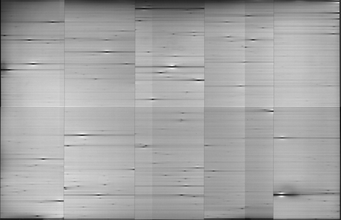
Figure 1: Thin-film module EL image. A module consists of 150 cells (positioned horizontally) connected in series. The cells are separated by interconnection lines (horizontal dark lines). The module consist of several submodules separated by vertical isolation lines, which appear dark in the EL image. The EL image is stitched (there are 1 horizontal and 3 vertical stitch lines); overall intensities of different patches of images are different. These intensity differences are attributed to metastable changes during the measurement.

As mentioned before, every EL image consists of several stitched images. Different stitched parts of the image have different overall intensities (see Figure 1). This is attributed to the metastable behaviour of CIGS solar cells, where the electrical properties of the cell can change during the measurement.

In order to obtainmanual labelling a labelled dataset we segment images manually. This work is done using two different image editor programs. Firstly, we use the GNU Image Manipulation Program (GIMP) [32] to create binary masks of various defects locations, where the defect pixels are manually marked using a drawing pad and a digital stylus. Alternatively, we use the ThinFia [33] program that is designed to identify defects in EL images by introducing a grid-mesh. thinfia and gimpThe ThinFia program was developed within the PEARL-TF project. A general image processing program such as GIMP requires more time to segment an image, comparing to the ThinFia, however, smaller defects are segmented more accurately in GIMP. The annotations for droplets and shunts are each performed by a single person, and thus the inter-annotator agreement has not been considered.inter-annotator

In the image database we focus on the segmentation of “shunts”. Shunts are characterized by a more conductive connection between the front and back electrodes than the normal solar cell structure (i.e. the solar cell structure is damaged or missing). There are many causes for shunts. Commonly shunts originate from debris of the copper evaporation source or pinholes in the CIGS absorber [34, 35]. Figure 2 (right) depicts a shunt defect. Shunts generally appear as dark areas with a gradient in intensity away from the actual defect location. The dark area is confined to the area of one cell. Severe shunts may also completely darken a cell stripe, in which case often the neighboring cells exhibit bright areas in the vicinity of the shunt [36]. Shunts are generally relevant to the solar module performance, in particular under low light conditions [37].

In addition to shunts we noticed the CIGS modules often exhibit “droplets” in the EL images. Figure 2 (left) shows a detail of droplets. The appearance of droplets resembles water stains and thus we speculate these structures originate from the chemical bath deposition. At this point it is unknown what the impact of droplets is on the module performance, however, the bright appearance imply a local change in quantum efficiency according to the reciprocity relations between luminescence and quantum efficiencytypo: page 3 efficiency [38].

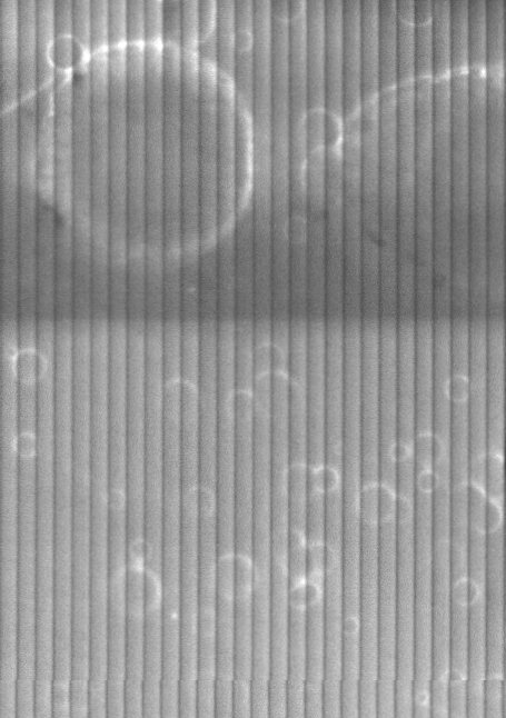
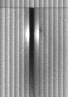
Figure 2: Example of droplets (left) and a shunted area (right). Here the cells are shown vertically.

In totaltotal images, we have about 6000 unlabelled, 142 labelled module images with shunts, and 14 labelled module images with droplets. The manual segmentation of droplets in an image is particular laborious, hence only few images are available.

training and testing datasets All labelled images are split randomly onto a training and a testing datasets. The training dataset consists 106 labelled shunts and 8 labelled droplets images. The testing dataset contains 24 labelled shunt and 3 droplets images. In addition we evaluate the final model using the remaining 12 images with shunts and 3 images with droplets.

The labelled dataset is available online, [39].

IV Methods

In this section we review methods that we use to build segmentation models. The encoder-decoder deep neural network architectures, [40], are commonly used in the semantic image segmentation problems, [30, 29, 25, 24]. We build multiple models by combining different encoder and decoder parts in the neural network architecture.

In order to populate our training data set we apply various transformations (data augmentation) to the original EL images.

After several models are trained, we compute segmentation on the test images and compute several performance metrics. It is important to establish a baseline for the evaluated metrics, as manual labelling has a significant human bias and differs for different types of defects.

The final model is obtained by means of using the multi-objective optimization technique.

It should be noted here, that the encoder-decoder models used here solve a general image segmentation problem, and hence can be applied to arbitrary images, as long as there exist a training dataset of sufficient size. For instance, these methods can be applied to different defects, different types of images (e.g. IR, PL, UVFL) or PV technologies (e.g. crystalline modules).

Our current approach is only restricted by the size of the input image patch and information contained in it. Therefore, defects that are larger than the input image patch can be problematic to identify.

IV-A Model architectures

For our segmentation models we utilize the encoder-decoder neural network architecture. These networks consist of two parts: the contraction part (or encoder) and the symmetric expansion part (or decoder). The encoder compresses information content of an arbitrarily high-dimensional image into a feature vector. The decoder gradually upscales the encoded features back to the original resolution.

Figure 3 schematically demonstrates a typical structure of the encoder-decoder architecture. Each block represents an output of the convolutional layer, with the data flow going from left to right. The arrows represent the skipping links, where the input for the layer is copied from the encoder to the decoder parts. Different networks may have different number of layers, skipping connections and different activation functions.

Figure 3: Schematic representation of an encoder-decoder architecture. The left-hand side image is an input image patch that is passed to a series of the computational layers. The right-hand side image is an output binary image. The arrows are skipping connection layers, where input is being copied directly from encoder to a decoder.

We take several popular networks and use parts of their architecture as an encoder or as a decoder. Combinations of encoders and decoders from different networks provide us with different segmentation networks. Furthermore, there are several tuning parameters available that allow us to generate even more segmentation models.

For the encoder part of our networks we use Mobile-net [41], ResNet [42], VGG-net [43] and U-net [44]. For the decoder part of our network we use U-net [44], FCN-net [45], PSP-net [46] and SegNet [47]. We use network implementations available in [48].

In order to be able to combine different encoder and decoder architectures we organize all encoder outputs to have 5 feature tensors. Different models have slightly different permissible input image sizes. The ResNet models require the input image dimension to be divisible by 32, the PSP-net models: divisible by 192. The Mobile-net models have the fixed input image size of $224\times 224$ pixels.

Table I summarizes the combinations of the encoder and decoder models. Some encoders and decoders have a tuning parameter. tuning parameters The ResNet, VGG-net, U-net have the size of the input image as an input parameter. We select between either $256\times 256$ and $512\times 512$. The SegNet’s parameter is the number of upsampling routines, see [47]. The FCN-net’s parameter has a single parameter: number of features, that can be equal $8$ or $32$. Combinations of different encoders and decoders with the choice of several tunable parameters provide us with a choice of 34 trainable modelstuning parameters result in models, i.e. we treat a single model with tuning parameters as several independent models corresponding to different choices of tuning parameters. Some of the FCN-net models with 32 layers are discarded as they require too much memory.

Table I: Various combination of encoder and decoder networks

Encoder	Decoder
Mobile-net	PSP-net
ResNet
VGG-net
Mobile-net	SegNet
ResNet
U-net
VGG-net

Encoder	Decoder
Mobile-net	U-net
ResNet
VGG-net
U-net
Mobile-net	FCN-net
ResNet
VGG-net
U-net

All models work with input image patches that are smaller than a typical EL image. The size of the input image regulates the information that is used for defect forecast. As shunts defects and droplets have a local nature, we select a square image patch size with an edge length varying between 15 and 30 times the cell width.

IV-B Data augmentation

We apply data augmentation to the training data set. The data augmentation is performed in order to increase the number of images to train our models with. This is particularly important for recognizing droplets as we have few labelled images to train with.

For the data augmentation, it is important to note that convolutional neural networks are able to incorporate spatial information in its model, however, they are not equivariant to scale and rotation transformations. Thus, the augmentation of data must entail scaling and rotation operations in order to boost the ability of the network to generalize, [40].

We organized data augmentation procedures in a pipeline of data augmentation generators. A generator accepts an image as its input and outputs a list of augmented images. Every image in the output is “piped” to the following generator in the pipeline. Thus, a single input image generates a series of augmented output images.

Every data augmentation generator has a set of tunable parameters. These parameters regulate the properties of the generated output images, such as size and transformation severity.

First augmentation transformation we perform are done on the original pair of EL and the corresponding label images. An image is re-sized preserving the aspect ratio, with the scaling factors ranging in the interval $[0.7,1.3]$. This scaling operation allows to populate the training dataset with examples of modules of slightly different cell sizes. After scaling, we perform mirroring of the image with respect to the vertical and horizontal axes, and apply the following contrast transformation to the EL image:

$$\big{(}(1-\alpha)M-(1+\alpha)m\big{)}\frac{I-m}{M-m}+m(1+\alpha),$$ (1)

where $M$ and $m$ are the maximum and the minimum values of the image, $\alpha$ is selected in a range of values $[-0.4,0.4]$.

Our segmentation models use a particular dimension of the input image. For example, as mentioned before Mobile-net accepts only images with the width and height of 224 pixels, and the dimensions of the ResNet should be divisible by 32. For this reason the final generator in the pipeline generates the subimages of the required dimensions. The subimages are generated using a sliding window of the selected size. The window shift is chosen to be 50 pixels, thus, we obtain overlapping subimages.

The ResNet networks input image size is chosen to be equal of width and height $256$ and $512$ pixels, the Mobile-net network — 224 pixel and the PSP-net network — 192 pixels.input

The defects are distributed in a non-uniform way. Therefore, to have a representative sample, we select only those subimages that contain at least 200 pixels corresponding to a defectaugment filter. All the training images are shuffled, so that, a particular order of the generator output does not play any role.

IV-C Training

We use the transfer learning technique [40], i.e. we use the pre-trained model on an unrelated dataset of images, and fine-tune it to adapt to the new task. We use weights that were pre-trained on the ImageNet dataset, [49]. The weights for various networks are accessible in [50].

In our training we use the dropout regularization technique, with the dropout rate chosen $0.2$; as well as the batch normalization technique. The latter method allows to normalize the inputs of every layer in the network, that helps reduce effect of the so-called covariance shift, [51].

For the loss function we use the categorical cross-entropy function, [40]loss function. We use the AdaDelta optimizer [52], as it requires no manual setting of a learning rate; it is robust to large gradients, noise architecture choice and insensitive to hyperparameters. The number of epochs is chosen to equal 100 with 512 gradient steps in each epoch. The training process stabilizes by this time, with no overfitting being observed in accuracy metrics evaluated on a testing dataset.

IV-D Accuracy metrics

To compare the trained segmentation models we compute performance metrics on pairs consisting of a segmented image and the corresponding ground truth mask.

The first performance metric is a common Jaccard index, [53]. Given two binary masks $A$ and $B$, the Jaccard index is defined by $J(A,B)\coloneqq\frac{|A\cap B|}{|A\cup B|},$ where $|A|$ denotes the number of non-zero elements in the binary mask $A$. The Jaccard index attains values in the interval $[0,1]$, where $0$ corresponds to the case when the binary masks $A$ and $B$ do not have common values.

We evaluate an index on a set of test images, thus obtaining a sample of index values for each model. our empirical finding remove The Jaccard index can be used to discover very bad-performing models, however, it cannot identify a significant difference between models.visuallydifferentmodels We conjecture that this happens because the Jaccard index reflects not only errors in defect locations, but also in its shape.

To address this drawback we introduce a second set of performance metrics, that ignores the shape information and focuses on the accuracy of the defects identification. We assume here that a single connected component in a segmented image constitutes a defect.

To this end, let $A$ and $B$ be two binary masks, and $K(A)$ is a set of connected components in $A$. Define the component instance function

$$I(A,B)\coloneqq\frac{\big{|}x\in K(B)\,|\,\exists y\in K(A\cap B):y\cap x\neq\emptyset\big{|}}{|K(B)|}.$$ (2)

Note that the component instance function attains values in the interval $[0,1]$, as the nominator is always less or equal than denominator. The connected components are computed using the labelling algorithm, [54].

The instance function is not symmetric, and if $A$ is a segmentation output and $B$ is the ground truth, then $I(B,A)$ can be interpreted as a precision index and $I(A,B)$ can be interpreted as a recall index.

The precision and recall are typical metrics computed in classification problems. In our case they can be interpreted in the following way. true location explanationThe precision is the proportion of correctly identified defects among all locations identified by a model, while the recall is the fraction of all defects that were identified by a model.

The component instance function formalises the meaning of a single defect by using the notion of a connected component. The defect is identified correctly, if the component on the ground truth image and the segmented image have a non-zero intersection.

IV-E Metrics baseline identification

A typical accuracy metric (or index) attains values in the interval $[0,1]$, where $0$ corresponds to a bad segmentation and $1$ to a perfect segmentation. In practice, however, the value of $1$ cannot be achieved. The reason for that in our case is the lack of clearly defined ground truth segmentation.

This happens due to several reasons. Firstly, when a defect expresses itself with a smooth gradient change in the image pixel value intensity, the beginning of the defect can be ambiguousambiguous labelling. For example, this can be observed in a shunted area, see Figure 2 (right). A shunt can be a microscopic defect, but on an EL image it induces a much larger darkened region with a smooth gradient change. Secondly, there can be too many defects to label them manually with high accuracy. For example, Figure 2 (left) shows a part of a module with so-called droplets.

establishing a baseline Therefore, to identify the values of the metrics that can be considered as good, we propose the following procedure. A set of images are segmented manually twice by the same person. A sufficient amount of time (more than 1 week) is taken between the first and second manual segmentation.double segmentation baseline The resulting segmentation images are evaluated using the performance metrics, to obtain the baseline values for the metrics.

IV-F Model selection

Combinations of different encoder and decoder networks with different tuning parameters yield a set of segmentation models. In this section we address the question of how to select the best model from this set, and discuss related problems.

Previously, we defined several metrics that are capable of measuring the quality of the segmentation given a manually segmented image. A two-stage procedure as described above allows to identify the baseline values for each metric, which allows to normalize the values and avoid the human bias incorporated in the raw metrics.

However, it is not possible to select the best model based on a single metric value. Firstly, from a sample of test images a single metric cannot significantly distinguish between several well performing models. At the same time, a visual inspection of the evaluations of this model indicate that models differ. Secondly, different metrics incorporate different information in its values. For example, the precision metric $I(B,A)$ measures how accurate are the identified defects by the model, whereas the recall metric $I(A,B)$ measures the total percentage of all identified defects.

Therefore, in order to address these problems we propose the following heuristic two-stage procedure. In the first step we select a set of models using a multi-objective optimization similar to the one used by [24], [24]. We use our precision and recall indices as the targets in the multi-objective optimization. In the second step, from a set of chosen models we select the final model using the Jaccard index. modelselectionfrompareto

V Results

To compute evaluation of a full sized module image we compute evaluation on a set of overlapping subimages, where the size of each subimage equals to the selected model input image size. Note that this introduces a limit on the size of the structures that can be detected as the model cannot properly detect structures larger than the subimage size. The resulting segmented image patches are combined with the overlapping borders being removed.

overlapping We overlap images by selecting a shift of 10 pixels less than what would be needed for producing subimages without an overlap. The width of the removed subimage borders equals to 5 pixels. The areas on the borders of the original image are not overlapped, and hence not removed.

The purpose of overlapping is to mitigate an incorrect segmentation close to the edges of the image patches. This problem is observed frequently in the FCN-net networks.

After the image augmentation pipeline we have about 15000 training images for shunts and 5000 training images for droplets.augment number images

Below we discuss the model selection for shunts and droplets, we demonstrate examples of shunts and droplets segmentation for the selected models, and provide details on the implementation and time required for the segmentation.

V-A Model selection

Figure 4 showsfigure 4 and 5 clarifications the estimated median of the precision and recall indices for each of the model for droplets (top figure) and shunts (bottom figure). The model evaluations are performed on a testing dataset that was not used during the training processevaluation on testing dataset.

The black line is the Pareto frontier of precision/recall multi-objective optimization for the droplets and shunts models. The Pareto frontier allows to select 6 models for droplets and 7 models for shunts. The red circle indicate the model on the frontier that maximizes the Jaccard indexmodelselectionfrompareto2. For the shunts the best model is Mobile-net-encoder and FCN-net-decoder, and for the droplets the best model is VGG-net-encoder and U-net-decoder.

Note that the estimated baseline for the precision and recall indices are equal 0.8 for both shunts and droplets, the Jaccard index baseline equals to 0.24 for shunts and 0.34 for droplets.baseline estimated

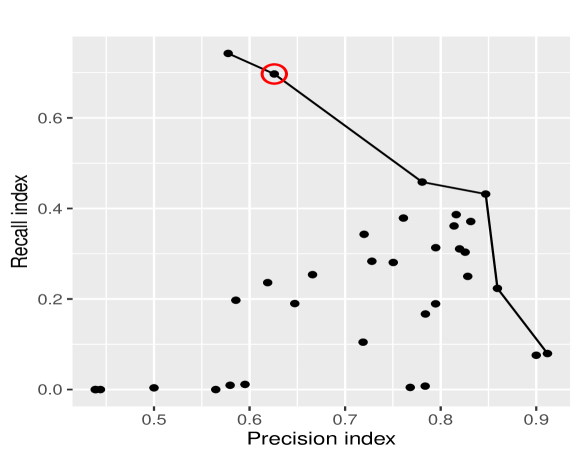
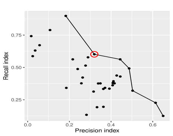
Figure 4: Pareto frontier for the droplets (top) and shunts (bottom) models

tuning parameters 2 All selected models have an input image of dimensions $256\times 256$ pixels (one of the tuning parameter for FCN-net and U-net), and the kernel size of the FCN-net network equals to 8.

final evaluation We perform a final evaluation on a set of images disjoint from training and testing images. Table II summarised the median value of the precision, recall and Jaccard indices evaluated on 24 shunts and 3 droplets images.

Table II: Final evaluation of the selected models

	Precision	Recall	Jaccard
Shunts	0.35	0.55	0.19
Droplets	0.61	0.68	0.27

In Figure 5 we show examples of the segmentation of droplets and shunts on two thin-film modules using the selected models. On the left side of the figures is shown the original image. On the right side is the binary mask of the segmentation. In the centre is shown an original image overlayed with the binary mask.

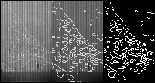
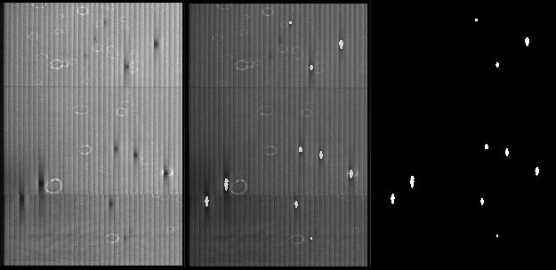
Figure 5: An example of droplets (top) and shunts (bottom) segmentation

V-B Segmentation examples and heat-maps

We apply the segmentation model for droplets and shunts for each EL image in our database. By evaluating an average of the computed binary segmented image, we obtain so-called heat maps. Figure 6 depicts heat maps based on 6000 EL images for droplet (top figure) and shunts (bottom figure) locationsCIGS subset. The brighter areas correspond to locations where defects have a higher probability of occurrence. The heat maps are given with a scale that maps pixel value in heat map images to a probabilityheatmap probability of shunts or droplets in that pixel. Note, that the scale is logarithmic in Figure 6 (bottom), with the $1\%$ of the brightest observations are shown as the white color.

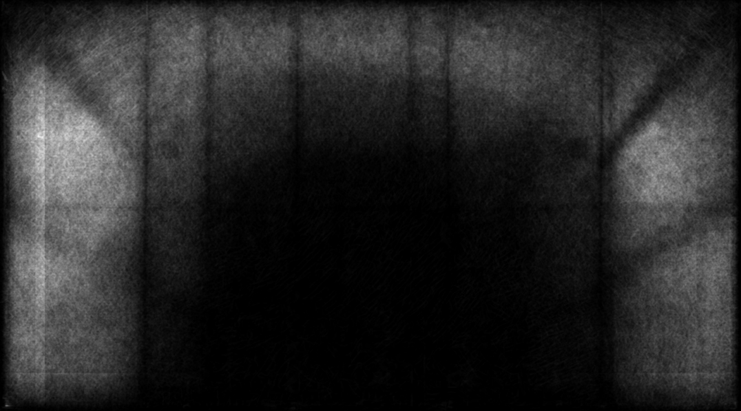
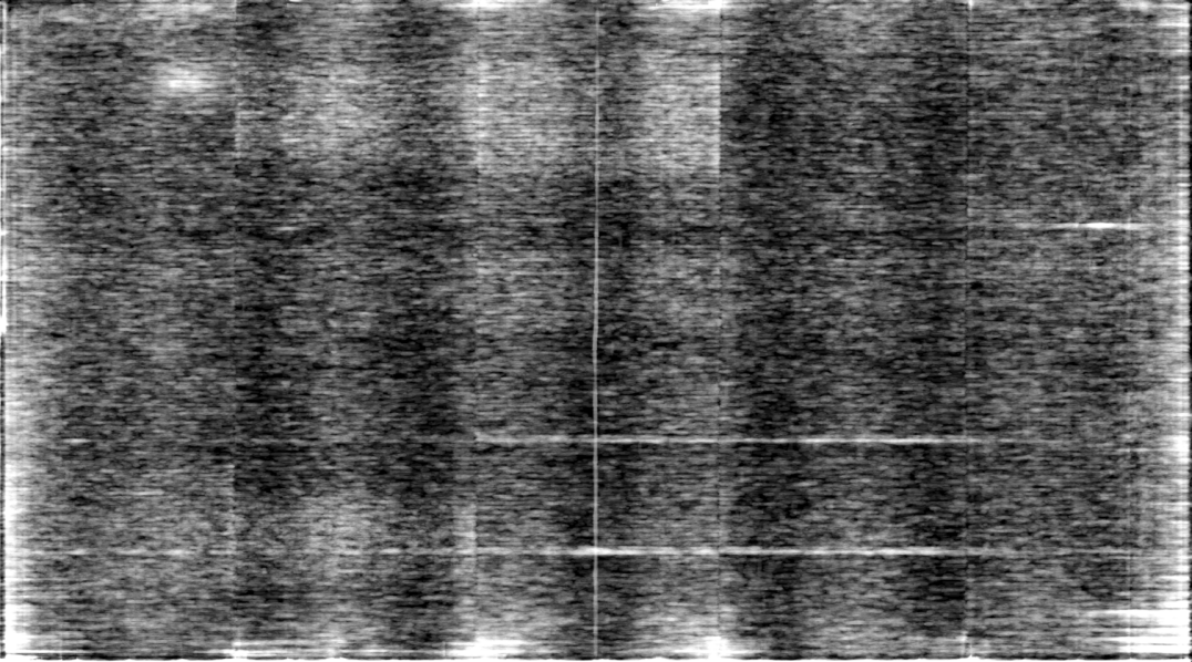
Figure 6: Heat map of droplets (top) and shunts (bottom) locations. The intensity scale indicates the probablity a pixel is marked as a droplet or a shunt.

The droplets in Figure 6 (top) expresses a clear structure where droplets are distributed along a broad arc along three edges of the module. In the brighter areas of the arc, the probability that a pixel is marked as a droplet is about 2.5% (148 times in 6000 imagesnumber of images in heatmap). The droplets do not occur in the center of the modules. Furthermore, there are several dark lines where fewer droplets are detected. The vertical and horizontal dark lines appear to be interference of vertical isolation lines in the modules as well as stitching lines in the image. However, the diagonal lines do not correspond to any obvious structure in the images that may interfere with droplet detection. We infer the diagonal lines have a physical origin.

The heat map of shunts is shown in Figure 6 (bottom). There is a great number of features to be seen, such as a clear banded structure, high concentrations at certain edges and locations, such as at the bottom edge where at the isolation lines high concentrations of shunts are detected. Two cell stripes in the bottom half of the module are more often shunted. The stitching lines do not show up and thus do not seem to interfere with shunt detection. The isolation lines are associated with more detected shunts. However, only parts of the isolation lines exhibit a larger concentration of shunts and not all isolation lines are equally affected. For this reason we believe the higher shunt probability around the isolation lines is no artifact. There is a bright vertical line in the center. This line does not correspond to the position of an isolation line or stitching line. Note that in Figure 5 a slightly darker vertical line is visible at the same position. However, in this example no shunts are detected along this line. In other EL images this darker line is not present (e.g. in Figure 1). The origin of this line is unclear.

We would like to note that many features in Figure 6 are rather subtle, and that these features only become visible when an average of a large number of images is computed. Furthermore, some of these features are quite certainly performance and reliability relevant (e.g. positions where shunts are likely to occur). We thus believe the extraction of such features can give manufacturers a better insight in their production process and thus contribute to process optimization and quality control.

V-C Correlation to performance data

correlation to performance Using the computed segmentation of EL images it is possible to correlate difference characteristics of the discovered defects in EL images and the performance of the modules.

Shunts originate from holes in the CIGS absorber, [34, 35], and primarely affect the low-light performance and the shunt resistance of PV modules [37]. A lower shunt resistance is expected to affect the fill factor and the slope of the IV characteristics around short circuit conditions. Note that it is a common practise in industry to count shunts in order to asses module quality.

Figure 7 shows a correlative plot between the slope of the IV curve near the short-circuit point and the number of the discovered shunts. The figure reveals no significant correlations between the variables. Unfortunately, we do not have low-light performance data for the correlation.

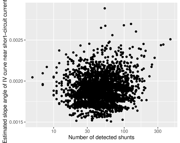
Figure 7: Slope of the IV curve near the short circuit current point versus number of shunts detected in the corresponding EL image.

Our study indicated that there are no significant correlations between size and amount of defects and the module performance data. Detailed discussion on the correlations between the discovered defects and performance of the modules is beyond the discussed topic of this paper.

VI Conclusions and outlook

In this paper, we applied the encoder-decoder deep neural networks in order to perform semantic segmentation of EL images of thin-film modules. The framework is general and applicable to other types of defects, PV images (e.g. thermography), as well as PV technologies.

We demonstrated the use of encoder-decoder deep neural networks to detect shunt-type defects and so-called droplets in thin-film CIGS solar cells. Several models are tested using various combinations of encoder-decoder layers. A method is proposed to select the best model based on the collection of metrics that evaluate different accuracy characteristics.

We show exemplary results for our selected best models of shunts and droplets. Furthermore, we analyzed a database with 6000 images of CIGS modules, all of one module type and one manufacturer. We show heat maps depicting the probability of a shunt or droplet occurring at a certain location in the solar module. The results show that the systematic segmentation of a large volume of images can reveal subtle features which cannot be inferred from studying individual images. Thus, we argue this type of segmentation models may aid process optimization and quality control by manufacturers.

Image segmentation methods is an active field of research, and there are several ways our approach can be extended. Firstly, the ensemble learning technique can be used to combine several segmentation models together with an aim to improve the model accuracy. Secondly, one can use the Generative Adversarial type of Neural networks (GAN) that can learn the defining features of the sample of images. The segmentation models can be then built on top of the constructed network.

Lastly, we remark that the code is available upon request, and the labelled dataset is available online, see [39].code available and training data

References

- [1] Matthias Demant, Patrick Virtue, Aditya S Kovvali, Stella X Yu and Stefan Rein “Deep learning approach to inline quality rating and mapping of multi-crystalline Si-wafers” In 35th European Photovoltaic Solar Energy Conference and Exhibition, 2018, pp. 814–818
- [2] Sergiu Deitsch, Claudia Buerhop-Lutz, Andreas Maier, Florian Gallwitz and Christian Riess “Segmentation of Photovoltaic Module Cells in Electroluminescence Images” In arXiv preprint arXiv:1806.06530, 2018
- [3] Sergiu Deitsch, Vincent Christlein, Stephan Berger, Claudia Buerhop-Lutz, Andreas Maier, Florian Gallwitz and Christian Riess “Automatic classification of defective photovoltaic module cells in electroluminescence images” In Solar Energy 185 Elsevier, 2019, pp. 455–468
- [4] Aline Kirsten Vidal Oliveira, Mohammedreza Aghaei and Ricardo Rüther “Automatic Fault Detection of Photovoltaic Array by Convolutional Neural Networks During Aerial Infrared Thermography” In 36th European Photovoltaic Solar Energy Conference and Exhibition, 2019
- [5] Ahmad Maroof Karimi, Justin S Fada, Mohammad Akram Hossain, Shuying Yang, Timothy J Peshek, Jennifer L Braid and Roger H French “Automated Pipeline for Photovoltaic Module Electroluminescence Image Processing and Degradation Feature Classification” In IEEE Journal of Photovoltaics 9.5 IEEE, 2019, pp. 1324–1335
- [6] Evgenii Sovetkin and Ansgar Steland “Automatic processing and solar cell detection in photovoltaic electroluminescence images” In Integrated Computer-Aided Engineering IOS Press, 2019, pp. 1–15
- [7] IEA “Review of failures of photovoltaic modules—report IEA-PVPS T13-01: 2014”, 2014
- [8] Du-Ming Tsai, Chih-Chieh Chang and Shin-Min Chao “Micro-crack inspection in heterogeneously textured solar wafers using anisotropic diffusion” In Image and Vision Computing 28.3 Elsevier, 2010, pp. 491–501
- [9] Said Amirul Anwar and Mohd Zaid Abdullah “Micro-crack detection of multicrystalline solar cells featuring shape analysis and support vector machines” In IEEE International Conference on Control System, Computing and Engineering, 2012, pp. 143–148 IEEE
- [10] Said Amirul Anwar and Mohd Zaid Abdullah “Micro-crack detection of multicrystalline solar cells featuring an improved anisotropic diffusion filter and image segmentation technique” In EURASIP Journal on Image and Video Processing 2014.1 Springer, 2014, pp. 15
- [11] Du-Ming Tsai, Shih-Chieh Wu and Wei-Chen Li “Defect detection of solar cells in electroluminescence images using Fourier image reconstruction” In Solar Energy Materials and Solar Cells 99 Elsevier, 2012, pp. 250–262
- [12] Du-Ming Tsai, Shih-Chieh Wu and Wei-Yao Chiu “Defect detection in solar modules using ICA basis images” In IEEE Transactions on Industrial Informatics 9.1 IEEE, 2012, pp. 122–131
- [13] T. Sun, C. Tseng and M. Chen “Electric contacts inspection using machine vision” In Image and Vision Computing 28, 2010, pp. 890–901
- [14] Din-Chang Tseng, Yu-Shuo Liu and Chang-Min Chou “Automatic finger interruption detection in electroluminescence images of multicrystalline solar cells” In Mathematical Problems in Engineering 2015 Hindawi, 2015
- [15] Akash Singh Chaudhary and DK Chaturvedi “Efficient Thermal Image Segmentation for Heat Visualization in Solar Panels and Batteries using Watershed Transform” In International Journal of Image, Graphics and Signal Processing 9.11 Modern EducationComputer Science Press, 2017, pp. 10
- [16] Genevieve C Ngo and Erees Queen B Macabebe “Image segmentation using K-means color quantization and density-based spatial clustering of applications with noise (DBSCAN) for hotspot detection in photovoltaic modules” In IEEE Region 10 Conference (TENCON), 2016, pp. 1614–1618 IEEE
- [17] Moath Alsafasfeh, Ikhlas Abdel-Qader and Bradley Bazuin “Fault detection in photovoltaic system using SLIC and thermal images” In 8th International Conference on Information Technology (ICIT), 2017, pp. 672–676 IEEE
- [18] Johannes Hepp, Florian Machui, Hans-J. Egelhaaf, Christoph J. Brabec and Andreas Vetter “Automatized analysis of IR-images of photovoltaic modules and its use for quality control of solar cells” In Energy Science & Engineering 4.6, 2016, pp. 363–371 DOI: 10.1002/ese3.140
- [19] T. Potthoff, K. Bothe, U. Eitner, D. Hinken and M. Köntges “Detection of the voltage distribution in photovoltaic modules by electromluminescence imaging” In Progress in Photovoltaics 18, 2010, pp. 100–106
- [20] Sachin Mehta, Amar P Azad, Saneem A Chemmengath, Vikas Raykar and Shivkumar Kalyanaraman “Deepsolareye: Power loss prediction and weakly supervised soiling localization via fully convolutional networks for solar panels” In 2018 IEEE Winter Conference on Applications of Computer Vision (WACV), 2018, pp. 333–342 IEEE
- [21] Santiago Salamanca, Pilar Merchán and Iván García “On the detection of solar panels by image processing techniques” In 25th Mediterranean Conference on Control and Automation (MED), 2017, pp. 478–483 IEEE
- [22] Jonathan Masci, Ueli Meier, Dan Ciresan, Jürgen Schmidhuber and Gabriel Fricout “Steel defect classification with max-pooling convolutional neural networks” In International Joint Conference on Neural Networks (IJCNN), 2012, pp. 1–6 IEEE
- [23] Lei Zhang, Fan Yang, Yimin Daniel Zhang and Ying Julie Zhu “Road crack detection using deep convolutional neural network” In IEEE International Conference on Image Processing (ICIP), 2016, pp. 3708–3712 IEEE
- [24] François Waldner and Foivos Diakogiannis “Deep learning on edge: extracting field boundaries from satellite images with a convolutional neural network” In arXiv preprint arXiv:1910.12023, 2019
- [25] Vladimir Iglovikov and Alexey Shvets “Ternausnet: U-net with vgg11 encoder pre-trained on imagenet for image segmentation” In arXiv preprint arXiv:1801.05746, 2018
- [26] “Inria Aerial Image Labeling Dataset” Accessed: 2019-12-17 URL: project.inria.fr/aerialimagelabeling
- [27] Mohammad Havaei, Francis Dutil, Chris Pal, Hugo Larochelle and Pierre-Marc Jodoin “A convolutional neural network approach to brain tumor segmentation” In BrainLes, 2015, pp. 195–208 Springer
- [28] Andre Esteva, Brett Kuprel, Roberto A Novoa, Justin Ko, Susan M Swetter, Helen M Blau and Sebastian Thrun “Dermatologist-level classification of skin cancer with deep neural networks” In Nature 542.7639 Nature Publishing Group, 2017, pp. 115
- [29] Mohamed Attia, Mohammed Hossny, Saeid Nahavandi and Hamed Asadi “Surgical tool segmentation using a hybrid deep cnn-rnn auto encoder-decoder” In IEEE International Conference on Systems, Man, and Cybernetics (SMC), 2017, pp. 3373–3378 IEEE
- [30] Baris Kayalibay, Grady Jensen and Patrick Smagt “CNN-based segmentation of medical imaging data” In arXiv preprint arXiv:1701.03056, 2017
- [31] “PEARL-TF project website” Accessed: 2019-12-01 URL: https://pearltf.eu/
- [32] The GIMP Development Team “GIMP”, 2019 URL: https://www.gimp.org
- [33] PI-Berlin “ThinFiA - Software Version provided and made by PI-Berlin”, 2018
- [34] B. Misic, B. E. Pieters, U. Schweitzer, A. Gerber and U. Rau “Defect Diagnostics of Scribing Failures and Cu-Rich Debris in Cu(In,Ga)Se2 Thin-Film Solar Modules With Electroluminescence and Thermography” In IEEE Journal of Photovoltaics 5.4, 2015, pp. 1179–1187 DOI: 10.1109/JPHOTOV.2015.2422143
- [35] Boris Misic “Analysis and Simulation of Macroscopic Defects in Cu(In,Ga)Se2 Photovoltaic thin film modules” 372, Schriften des Forschungszentrums Jülich. Reihe Energie und Umwelt / Energy and Environment Forschungszentrum Jülich GmbH, 2017, pp. 17–36
- [36] TMH Tran, BE Pieters, M Siegloch, A Gerber, C Ulbrich, T Kirchartz, R Schäffler and U Rau “Characterization of shunts in Cu (In, Ga) Se2 solar modules via combined electroluminescence and dark lock-in thermography analysis” In 26th European Photovoltaic Solar Energy Conference and Exhibition, 2011, pp. 2981–2985
- [37] Thomas Weber, Anton Albert, Nicoletta Ferretti, Margarete Roericht, Stefan Krauter and Paul Grunow “Electroluminescence investigation on thin film modules” In 26th European Photovoltaic Solar Energy Conf.(26th EU PVSEC), 2011, pp. 2584–2588
- [38] Uwe Rau “Reciprocity relation between photovoltaic quantum efficiency and electroluminescent emission of solar cells” In Phys. Rev. B 76 American Physical Society, 2007, pp. 085303 DOI: 10.1103/PhysRevB.76.085303
- [39] “PEARL TF-PV, thin-film modules, shunts and droplets” Accessed: 2020-07-15 URL: https://b2share.fz-juelich.de/records/e19fe0f0bc0e4f1b8e05b28e977934c9
- [40] Ian Goodfellow, Yoshua Bengio and Aaron Courville “Deep learning” MIT press, 2016
- [41] Andrew G Howard, Menglong Zhu, Bo Chen, Dmitry Kalenichenko, Weijun Wang, Tobias Weyand, Marco Andreetto and Hartwig Adam “Mobilenets: Efficient convolutional neural networks for mobile vision applications” In arXiv preprint arXiv:1704.04861, 2017
- [42] Kaiming He, Xiangyu Zhang, Shaoqing Ren and Jian Sun “Deep residual learning for image recognition” In Proceedings of the IEEE Conference on Computer Vision and Pattern Recognition, 2016, pp. 770–778
- [43] Karen Simonyan and Andrew Zisserman “Very deep convolutional networks for large-scale image recognition” In arXiv preprint arXiv:1409.1556, 2014
- [44] Olaf Ronneberger, Philipp Fischer and Thomas Brox “U-net: Convolutional networks for biomedical image segmentation” In International Conference on Medical Image Computing and Computer-Assisted Intervention, 2015, pp. 234–241 Springer
- [45] Jonathan Long, Evan Shelhamer and Trevor Darrell “Fully convolutional networks for semantic segmentation” In Proceedings of the IEEE Conference on Computer Vision and Pattern Recognition, 2015, pp. 3431–3440
- [46] Hengshuang Zhao, Jianping Shi, Xiaojuan Qi, Xiaogang Wang and Jiaya Jia “Pyramid scene parsing network” In Proceedings of the IEEE Conference on Computer Vision and Pattern Recognition, 2017, pp. 2881–2890
- [47] Vijay Badrinarayanan, Alex Kendall and Roberto Cipolla “Segnet: A deep convolutional encoder-decoder architecture for image segmentation” In IEEE Transactions on Pattern Analysis and Machine Intelligence 39.12 IEEE, 2017, pp. 2481–2495
- [48] “Image Segmentation Keras : Implementation of Segnet, FCN, UNet, PSPNet and other models in Keras” Accessed: 2019-12-01 URL: https://github.com/divamgupta/image-segmentation-keras
- [49] J. Deng, W. Dong, R. Socher, L.-J. Li, K. Li and L. Fei-Fei “ImageNet: A Large-Scale Hierarchical Image Database” In CVPR09, 2009
- [50] “Trained image classification models for Keras” Accessed: 2019-12-01 URL: https://github.com/fchollet/deep-learning-models/releases/
- [51] Sergey Ioffe and Christian Szegedy “Batch normalization: Accelerating deep network training by reducing internal covariate shift” In arXiv preprint arXiv:1502.03167, 2015
- [52] Matthew D Zeiler “ADADELTA: an adaptive learning rate method” In arXiv preprint arXiv:1212.5701, 2012
- [53] Cornelis Joost Van Rijsbergen “Information retrieval” Citeseer, 1979
- [54] Kesheng Wu, Ekow Otoo and Arie Shoshani “Optimizing connected component labeling algorithms” In Medical Imaging 2005: Image Processing 5747, 2005, pp. 1965–1976 International Society for OpticsPhotonics