Diagnosing First and Second Order Phase Transitions with Probes of Quantum Chaos

Abstract

We explore quantum phase transitions using two probes of quantum chaos: out-of-time-order correlators (OTOCs) and the $r$-parameter obtained from the level spacing statistics. In particular, we address $p$-spin models associated with quantum annealing or reverse annealing. Quantum annealing triggers first-order or second-order phase transitions, which is crucial for the performance of quantum devices. We find that the time-averaging OTOCs for the ground state and the average $r$-parameter change behavior around the corresponding transition points, diagnosing the phase transition. Furthermore, they can identify the order (first or second) of the phase transition by their behavior at the quantum transition point, which changes abruptly (smoothly) in the case of first-order (second-order) phase transitions.

1 Introduction

In recent years, out-of-time-order correlators (OTOCs) [1] have gained renewed interest, especially because of their connection with many-body quantum chaos and black hole physics [2, 3]. See [4], for a recent review. For works regarding the experimental measurement of OTOCs, see for instance [5, 6, 7, 8].

An OTOC is defined as

$$F_{VW}(t)=\langle W(t)V(0)W(t)V(0)\rangle\,,$$ (1.1)

where $V$ and $W$ are some simple operators and the expectation value is usually taken in a thermal state. The idea is that chaotic behavior leads to an early-time exponential suppression and the late-time vanishing of OTOCs, which happens for almost any choice of operators $V$ and $W$. On the other hand, the absence of chaos is expected to result in a non-universal, operator-dependent behavior of $F_{VW}(t)$.

Another way to characterize quantum chaotic behavior is through the statistics of the spacing between consecutive energy eigenvalues, which is usually known as level spacing statistics. In chaotic systems, the level spacing statistics obeys a Wigner-Dyson distribution [9], while in integrable systems it follows a Poisson distribution [10, 11]. We can also study the so-called $r$-parameter statistics, which is computed from the level spacing information. The average $r$-parameter takes different values depending on whether the system is chaotic or integrable. See Sec. 4 for more details.

The level spacing statistics is defined at zero temperature and involves time-scales much bigger than the ones involved in the behavior of OTOCs, which are usually computed at finite temperature. Despite these differences, both the level spacing statistics and the OTOCs can probe chaotic behavior, presumably capturing different aspects of it, due to the thermal nature of OTOCs.

Thermal effects can be removed by considering ground state OTOCs, in which the expectation value is taken in the ground state of the system. In this case, the OTOCs are completely controlled by the ground state physics [12] and may become sensitive to changes in the ground state, i.e., they may diagnose quantum phase transitions [12, 13, 14]. As far as we know, the relation between level spacing statistics and quantum phase transitions remains largely unexplored. It is then interesting to explore if the tools used to characterize level spacing statistics are also useful in diagnosing phase transitions. This is one of the goals of this paper. This could help to clarify the role played by chaos in quantum phase transitions.

Quantum phase transitions are transitions between different phases of matter that occur at zero temperature by variation of a non-thermal control parameter. Quantum phase transitions found applications in the description of several properties of condensed matter systems [18], as well as in quantum computation algorithms. In this work, we will be interested in quantum phase transitions that are triggered by a method of adiabatic quantum computation known as quantum annealing.

Quantum annealing [19] is a meta-heuristic quantum method for solving combinatorial optimization problems and could be as powerful as universal computation when a system with a non-stoquastic Hamiltonian evolves in an adiabatic way [20]. The conventional form of quantum annealing is done by the quantum mechanical time evolution of an initial state, which is the ground state of a transverse magnetic field. The initial phase consists of the uniform superposition of all possible classical states, which is called the quantum paramagnetic (QP) phase. In general, the system evolves into a different phase and the performance of a quantum annealer depends heavily on the choice of transition paths. According to the adiabatic theorem, the computational time that is needed to efficiently obtain the ground state is proportional to the inverse square of the minimal energy gap $\Delta$ between the ground state and the first excited state. A lot of examples indicate that $\Delta$ decays polynomially if a phase transition is second-order [21, 22], whereas $\Delta$ decays exponentially if it is first-order (although there are some exceptions [23, 24, 25]). Therefore, the problem in the case of systems with second-order phase transitions is efficiently solved. There are some models for which the first-order phase transitions can be avoided when a non-stoquastic Hamiltonian or reverse annealing [26] is used. The $p$-spin model we address in this article is a typical example (see also [27, 28]). The ground state of the $p$-spin model is ferromagnetic (F) and, depending on the path, the QP/F transition becomes first-order or second-order. In [29, 27], it is suggested that entanglement measures are good tools to analyse phase transitions of such a fully connected spin system.

In this work, we aim at diagnosing quantum phase transitions triggered by quantum annealing using two probes of quantum chaos, namely, OTOCs and the $r$-parameter statistics. The relation between the second-order phase transition and the time average of OTOCs is reported [12, 13, 14], but not proven in general. For a better understanding, it will be useful if we can check it in other examples. In addition, less is known about the relation between the order of the phase transition and the behavior of the OTOC. As far as we know, the relation between phase transitions and the average $r$-parameter has not been studied either. In this paper, we show that OTOCs and the average $r$-parameter not only detect the phase transition but also distinguish the order of the phase transition. To our best knowledge, our paper is the first work in the following aspects: (1) relating both first-order and second-order phase transitions with the dynamics of OTOCs and the $r$-parameter statistics, (2) using probes of quantum chaos to study quantum annealing or adiabatic quantum computing and (3) the Hamiltonians we employed are non-stoquastic, which means the models cannot be efficiently simulated by classical ways. Some stoquastic models are studied elsewhere [30, 31, 32, 33].

This article is organized as follows. In Sec. 2 we review and explain the phase transition associated with quantum annealing of the $p$-spin model. In Sec 3 we use the time average of OTOCs to characterize the QP/F transition. In Sec. 4, we study the $r$-parameter statistics and show that the average $r$-parameter is sensitive to the phase transition. In Sec. 5 we address phase transitions associated with reverse annealing and provide more evidence that they can be diagnosed by the time average of OTOCs. Finally, we present our conclusions in Sec. 6.

2 Model

Let us start with a Hamiltonian of adiabatic quantum computation

$$H(s)=sH_{\mathrm{T}}+(1-s)H_{\mathrm{I}},~{}~{}~{}~{}~{}~{}~{}s\in[0,1]\,,$$ (2.1)

where $H_{\mathrm{T}}$ is a target Hamiltonian and $H_{\mathrm{I}}$ is an initial Hamiltonian. They should not commute $[H_{\mathrm{I}},H_{\mathrm{T}}]\neq 0$. As an initial Hamiltonian we use the widely used transverse magnetic field [19, 20]:

$$H_{\mathrm{I}}=-\sum_{i}^{N}X_{i}\,,$$ (2.2)

and as a target Hamiltonian let us consider the Hamiltonian of the $p$-spin model

$$H_{\mathrm{T}}=-N\left(\frac{1}{N}\sum_{i=1}^{N}Z_{i}\right)^{p}\,,$$ (2.3)

where $X_{i}$ and $Z_{i}$ denote, for example,

$$\begin{split}X_{1}&=\sigma_{x}\otimes I_{2}\otimes I_{2}\otimes\cdots\otimes I_{2}\,,\\ Z_{3}&=I_{2}\otimes I_{2}\otimes\sigma_{z}\otimes I_{2}\otimes\cdots\otimes I_{2}\,,\end{split}$$ (2.4)

with $\sigma_{x}=\scriptsize\left(\begin{array}[]{cc}0&1\\ 1&0\end{array}\right),\ \sigma_{z}=\left(\begin{array}[]{cc}1&0\\ 0&-1\end{array}\right)\,.$

The Hamiltonian (2.1) is stoquastic. We say a Hamiltonian is stoquastic if all off-diagonal matrix elements in the standard basis are real and non-positive, otherwise it is non-stoquastic [34]. We add a term that introduces non-stoquastic antiferromagnetic(AF) interactions

$$H_{\text{AF}}=+N\left(\frac{1}{N}\sum_{i}^{N}X_{i}\right)^{2}\,,$$ (2.5)

in such a way that

$$H(s,\lambda)=s(\lambda H_{\mathrm{T}}+(1-\lambda)H_{\text{AF}})+(1-s)H_{\mathrm{I}}\,.$$ (2.6)

Even though a non-stoquastic term is in general hard to simulate by quantum Monte Carlo due to the negative sign problem, sometimes it makes problems efficiently solvable by adiabatic quantum computation or quantum annealing [35]. Furthermore, it is believed that adding a stoquastic Hamiltonian to (2.1) is not helpful for quantum speedup.

The initial Hamiltonian ($s=0$) is $H(0,\lambda)=H_{\mathrm{I}}$ with any $\lambda$. The final Hamiltonian is chosen to be $H(1,1)=H_{\mathrm{T}}$. At the initial stage of annealing $(s=0)$, since $\sigma_{x}\ket{+}_{i}=\ket{+}_{i}$, the ground state $\ket{\psi_{\mathrm{QP}}}$ is a superposition of all possible $2^{N}$ states with an equal probability weight

$$\ket{\psi_{\mathrm{QP}}}:=\prod_{i}^{N}\ket{+}_{i}=\frac{1}{\sqrt{2^{N}}}(\ket{\uparrow\uparrow\cdots\uparrow}+\ket{\uparrow\uparrow\cdots\uparrow\downarrow}+\cdots+\ket{\downarrow\downarrow\cdots\downarrow})\,,$$ (2.7)

which we call the quantum paramagnetic (QP) phase. Here $\ket{\uparrow}$ and $\ket{\downarrow}$ denote eigenstates of $\sigma_{z}$ at each site, i.e., $\sigma_{z}\ket{\uparrow}_{i}=\ket{\uparrow}_{i}$ and $\sigma_{z}\ket{\downarrow}_{i}=-\ket{\downarrow}_{i}$. The ground state of the target Hamlitonian $H_{\mathrm{T}}$ is degenerated if $p$ is even so we consider the cases when $p$ is odd. Then the ground state of $H_{\mathrm{T}}$ consists of all spins pointing up

$$\ket{\psi_{\mathrm{F}}}:=\ket{\uparrow\uparrow\cdots\uparrow}\,,$$ (2.8)

which is the ferromagnetic (F) phase.

Hence, as $s$ increases, a phase transition from QP phase to F phase occurs. The corresponding order parameters are magnetizations

$$m_{x}:=\frac{1}{N}\sum_{i}^{N}\left\langle X_{i}\right\rangle\,,\qquad m_{z}:=\frac{1}{N}\sum_{i}^{N}\langle Z_{i}\rangle\,,$$ (2.9)

where the expectation value is obtained by the ground state at a given $s$. The first-order (second-order) phase transitions are defined by the discontinuity (continuity) of a given order parameter, respectively. Without the antiferromagnetic interactions ($\lambda=1$), it is known that this model costs exponentially long time to obtain the ground state of $H_{\mathrm{T}}$ due to a first-order phase transition [36]. The first-order phase transition can be avoided by strong enough antiferromagnetic interactions, with which the problem can be solved efficiently [35, 27, 37]. In fact, by studying the behavior of $m_{x}$ along the quantum annealing process, the authors of [35] showed that, for $p>3$, the system displays a first-order phase transition when $\lambda\gtrsim 0.4$, but the transition becomes second order for smaller values of $\lambda$. In their analysis, they consider a large $N$ approximation. This phase transition was also studied at large $N$ using a spin-coherent state technique [27], which gives results that are consistent with the analysis of [35].

In this section, we first reproduce some of the results of [35] at finite $N$ without using a large $N$ approximation. By performing a direct diagonalization of the Hamiltonian (2.6), we numerically compute the ground state expectation values in (2.9). This is an important step because we will compute OTOCs at finite $N$ in the subsequent sections and try to understand its large $N$ properties. Thus, we first need to find an optimal $N$ which can be taken as large enough with reasonable computing time.

(a) $N=11$, $p=11$, $\lambda=1.0$

(b) $N=11$, $p=5$, $\lambda=0.2$

Figure 1: Magnetizations $m_{x}$ and $m_{z}$ versus $s$ for $N=11$. There are the first order(a) or second order(b) phase transitions between the QP phase (2.7) and the F phase (2.8). The vertical dashed line indicates the transition point.

(a) $N=20$, $p=11$, $\lambda=1.0$

(b) $N=20$, $p=5$, $\lambda=0.2$

Figure 2: Magnetization $m_{x}$ versus $s$ for $N=20$. There are the first order(a) or second order(b) transitions between the QP phase (2.7) and the F phase (2.8). The first order phase transition is clearer when compared to Fig. 1(a), where we set $N=11$. The vertical dashed line indicates the transition point.

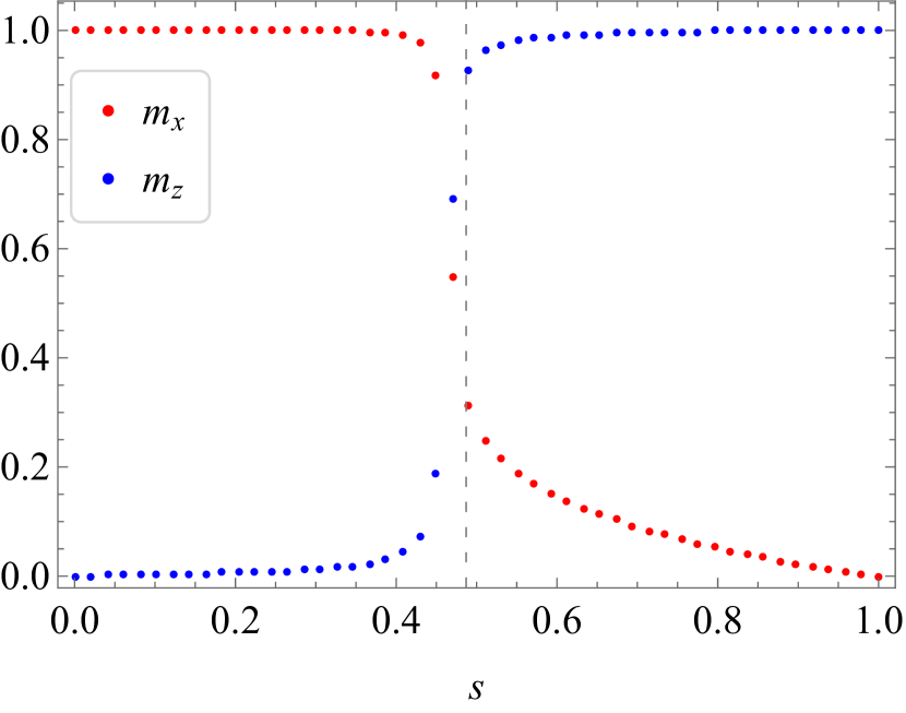
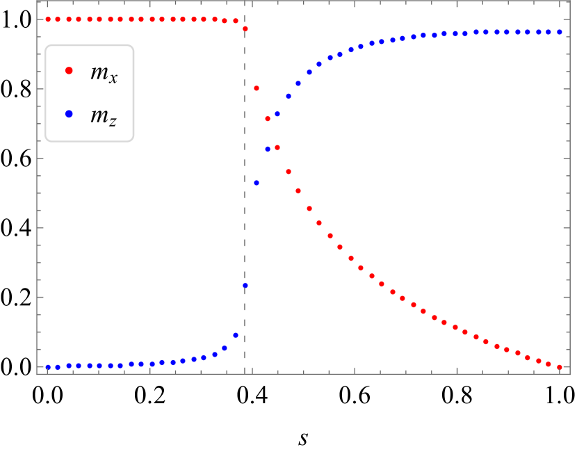
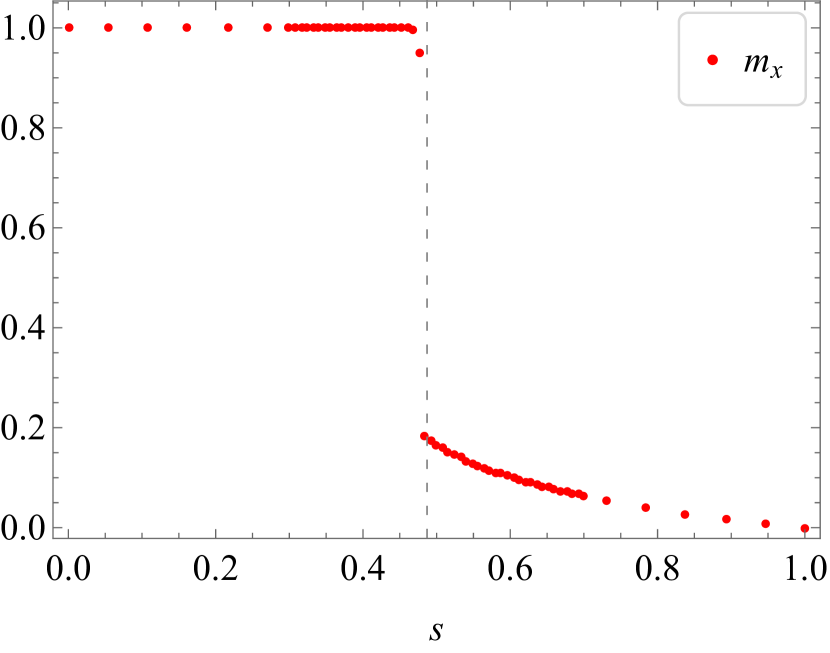
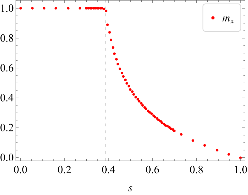
Fig. 1 shows the behavior of the magnetizations $m_{x}$ and $m_{z}$ as functions of $s$ for some values of $N$, $\lambda$ and $p$. As expected, at $s=0$ $m_{x}$ ($m_{z}$) starts from one (zero) and decreases (increases) to zero (a constant positive value) as we increase $s$. We chose $N=11$ for the sake of comparison because it is the optimal value we will use in the following OTOC computation. If $\lambda\gtrsim 0.4$ the transition is first-order while if $\lambda\lesssim 0.4$ the transition is second-order. To show this we choose $\lambda=0.2$ and $\lambda=1$. The feature of the first-order phase transition can be seen with $N=11$ in Fig. 1(a), but it is clearer for larger values of $N$. See Fig. 2 where we set $N=20$.

3 Diagnosing Quantum Phase Transition with OTOC

In the previous section we reviewed that the system described by the Hamiltonian (2.6) displays a quantum phase transition from a quantum paramagnetic (QP) phase to a ferromagnetic (F) phase as we change the parameter $s$ from 0 to 1. In this section, we study quantum phase transitions from the viewpoint of quantum chaos, in particular in terms of out-of-time-order correlators (OTOCs).

3.1 Short Review on OTOC

Here we provide a short review on OTOCs. For more details we refer to [4]. The OTOCs have the form

$$F_{VW}(t)=\langle W(t)VW(t)V\rangle\,,$$ (3.1)

where $V$ and $W$ are Hermitian and unitary local operators. In chaotic many-body systems, one expects $F_{VW}(t)$ to vanish at late times for almost any choice of operators $V$ and $W$.

The late-time vanishing of OTOCs is tied to the idea of scrambling of quantum information, which takes place in chaotic systems. Using the Baker-Campbell-Hausdorff (BCH) formula, we can write the Heisenberg operator as

$$W(t)=e^{iHt}We^{-iHt}=W+it\,[H,W]+\frac{(it)^{2}}{2!}[H,[H,W]]+\cdots\,.$$ (3.2)

At $t=0$, the operator only involves the local degrees of freedom associated with $W$. Under time evolution, higher order terms in the BCH become important, and $W(t)$ becomes more and more complicated as it starts to act non-trivially in a increasing number of degrees of freedom. In other words, the operator $W(t)$ ‘grows’ with time, and the initially local information gets scrambled into a non-local form.

The scrambling of the operator $W(t)$ can be probed by considering its commutator with some other, local operator, $V$. To avoid phase cancellations, one usually defines the double commutator

$$C(t)=\langle|[W(t),V]|^{2}\rangle\,,$$ (3.3)

which starts at zero and grows as $W(t)$ scrambles with an increasing number of degrees of freedom. After the so-called ‘scrambling time’, the operator $W(t)$ is scrambled with essentially all the degrees of freedom of the system, and $C(t)$ saturates to a constant value, which equals $2\,\langle VV\rangle\langle WW\rangle$. The double commutator is closely related to OTOCs. For unitary $V$ and $W$, the double commutator can be written as $C(t)=2(1-\text{Re}[F_{VW}(t)])$. Hence, the saturation of the double commutator after the scrambling time implies the vanishing of OTOCs. In contrast, in non-chaotic systems, one expects a non-universal behavior of the OTOCs, which in general depends on the choice of the operators $V$ and $W$. Moreover, the absence of thermalization in integrable systems is expected to lead to an oscillatory behavior of OTOCs.

The way $F_{VW}(t)$ approaches to zero is particularly simple in systems that display some sort of classical limit (e.g.: quantum mechanical systems that have a well-defined $\hbar\rightarrow 0$ limit or certain large-$N$ systems). In those cases, in an appropriate time window, the double commutator grows exponentially, i.e., $C(t)\sim e^{\lambda_{L}t}$, which is reminiscent of the divergence in the distance between initially nearby trajectories in the phase space of classically chaotic systems. In those cases, one can define a quantum Lyapunov exponent $\lambda_{L}$ characterizing the onset of chaos in the system. By contrast, in standard spin chains models with local interactions, $F_{VW}(t)$ does not have any sort of exponential behavior with time [41, 42], even for systems that are known to be strongly chaotic by other more conventional criteria for quantum chaos. This prevents the definition of a quantum Lyapunov exponent for those systems (see, however, [43]). Despite the absence of exponential behavior, one usually expects to distinguish chaotic and integrable systems by the late-time behavior of OTOCs, which vanishes in the case of many-body chaotic systems.

In finite-size systems, OTOCs do not decay exactly to zero at late times. In fact, it has been shown that the residual late-time value of OTOCs provides useful insights into the chaotic dynamics [40]. For energy-conserving chaotic spin chains, for example, the late-time value of the OTOCs scale as an inverse polynomial in the system size [40].

3.2 Ground state OTOCs

We are interested in ground state OTOCs

$$F_{VW}^{(0)}(t)=\bra{\phi_{0}}W(t)VW(t)V\ket{\phi_{0}}\,,$$ (3.4)

where $V$ and $W$ are Hermitian operators and $\ket{\phi_{0}}$ is the ground state of the total Hamiltonian $H=H(s,\lambda)$. In the following, we consider cases where $V$ and $W$ are non-local operators, like

$$S^{x}=\frac{1}{2}\sum_{i=1}^{N}\sigma^{x}_{i}\,,\quad\mathrm{or}\quad S^{z}=\frac{1}{2}\sum_{i=1}^{N}\sigma^{z}_{i}\,,$$ (3.5)

and also cases where $V$ and $W$ are local unitary operators, like $X_{i}$ or $Z_{i}$, for some site $i$ as in (2.4).

In both cases, the OTOCs show a qualitatively similar behavior, but the results for non-local operators tend to be more smooth. As an example, we show in Fig. 3 the time dependence of $F_{S^{x}S^{x}}^{(0)}(t)$ for increasing values of the annealing parameter $s$.

Figure 3: Time dependence of $F_{S^{x}S^{x}}^{(0)}(t)$ for increasing values of the annealing parameter $s$. Here we set $N=11$, $p=5$ and $\lambda=0.2$. The OTOC oscillates around a constant positive value that depends on the value of $s$.

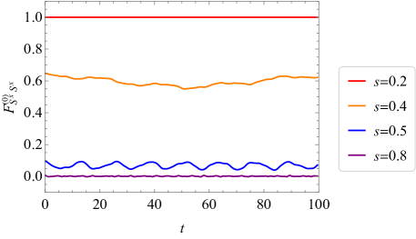
In the beginning of the annealing process, when $s<s_{c}$ (in this case, $s_{c}=0.385$) and the system is in the QP phase, $F_{S^{x}S^{x}}^{(0)}$ oscillates around one. After the phase transition to the F phase, for $s>s_{c}$, $F_{S^{x}S^{x}}^{(0)}$ oscillates around a constant (smaller than one) value that quickly decreases to zero as $s$ approaches one.

The above time-behavior indicates that the time-averaging OTOCs

$$\bar{F}_{VW}^{(0)}=\lim_{T\to\infty}\frac{1}{T}\int_{0}^{T}F_{VW}^{(0)}(t)\,dt\,,$$ (3.6)

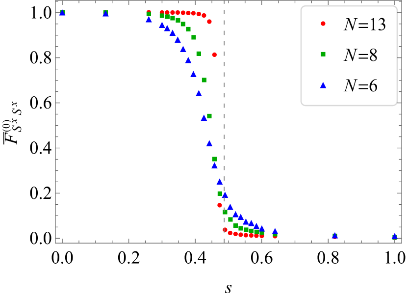
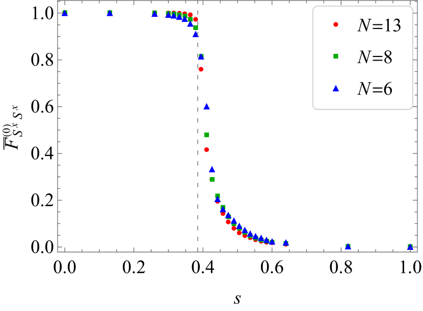
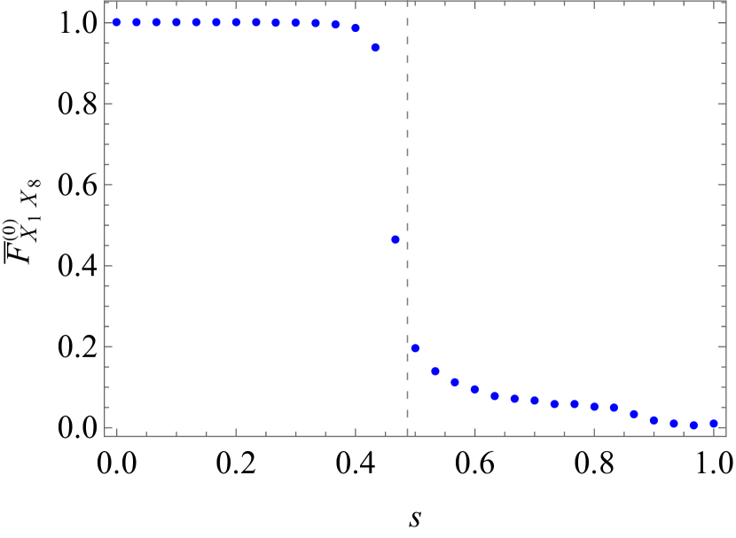
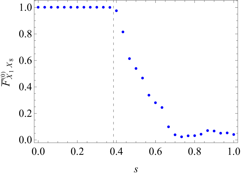
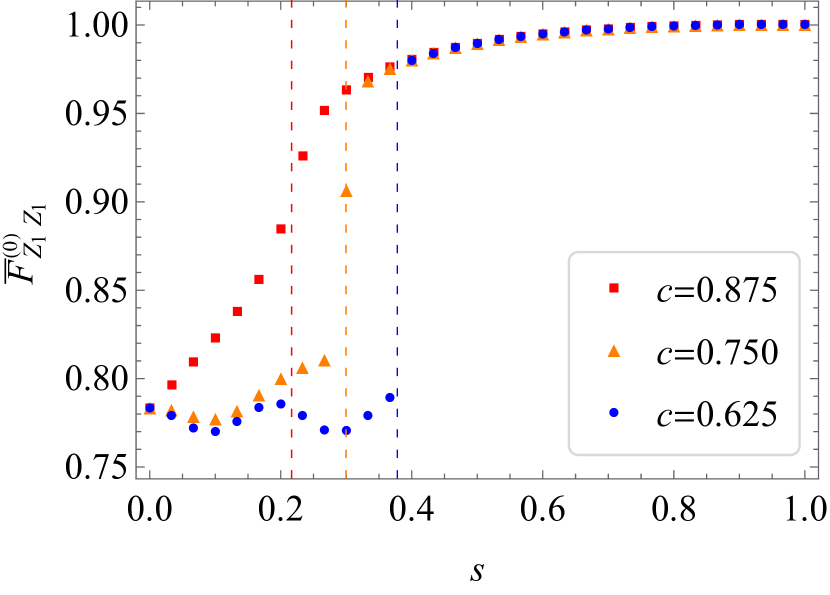
can diagnose the phase transition. We have checked that this is indeed true by studying the behavior of $\bar{F}_{VW}^{(0)}$ along the annealing process. Fig. 4 shows the behavior of $\bar{F}_{S^{x}S^{x}}^{(0)}$ as a function of the annealing parameter $s$. The time-averaging OTOC changes behavior across the quantum phase transition, whose transition points (estimated at large $N$) are indicated in the plots by vertical lines. The transition points of the second-order phase transitions obey the formula $s_{c}=\frac{1}{3-2\lambda}$ and those of the first-order phase transitions are numerically estimated in [27]. Those estimates become more and more precise as we consider larger values of $N$.

The choice of parameters for Fig. 4 is such that we have a first-order phase transition in Fig. 4(a), where $(p,\lambda)=(11,1)$, and a second-order phase transition in Fig. 4(b), where $(p,\lambda)=(5,0.2)$. The order of the phase transition is visible in the behavior of the time-averaging OTOC, specially when we consider the curves for $N=13$, where we can see that $\bar{F}_{S^{x}S^{x}}^{(0)}$ has a discontinuous (continuous) behavior at the quantum transition point in first-order (second-order) phase transitions.

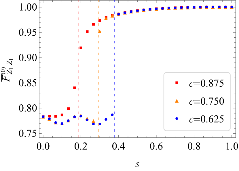
The diagnosis of the phase transition in terms of time-averaging OTOCs is not limited to a particular choice of operators. Fig. 5 shows that $\bar{F}_{S^{z}S^{z}}^{(0)}$ changes behavior around the quantum transition point, and also identifies the order of the phase transition. The same is true for time-averaging OTOCs involving local operators, e.g., $\bar{F}^{(0)}_{X_{1}X_{8}}$, as it is shown in Fig. 6. We have also checked that it is possible to detect the phase transition with different combinations, like $(V,W)=(Y_{i},X_{i}),\,(X_{i},Z_{i})$, etc. In this sense, we may say that the OTOCs provide a generalization of the order parameter, and thereby are useful to characterize a phase transition when the rigorous order parameter is unknown.

(a) $p=11,\lambda=1.0$

(b) $p=5,\lambda=0.2$

Figure 4: Time-averaging OTOCs $\bar{F}_{S^{x}S^{x}}$ versus the annealing parameter $s$. Here we set $N=6,8,13$. The phase transition is first-order for $(p,\lambda)=(11,1.0)$ and second-order for $(p,\lambda)=(5,0.2$). The transition points of the second-order phase transitions obey the formula $s=\frac{1}{3-2\lambda}$ and those of the first-order phase transitions are numerically estimated in [27].

(a) $p=11,\lambda=1.0$

(b) $p=5,\lambda=0.2$

Figure 5: Time-averaging OTOC $\bar{F}_{S^{z}S^{z}}^{(0)}$ versus the annealing parameter $s$. The transition points for each case are indicated by vertical lines. Here we set $N=11$.

(a) $p=11,\lambda=1.0$

(b) $p=5,\lambda=0.2$

Figure 6: Time-averaging OTOC $\bar{F}_{X_{1}X_{8}}^{(0)}$ versus the annealing parameter $s$. The transition points for each case are indicated by vertical lines. Here we set $N=11$.

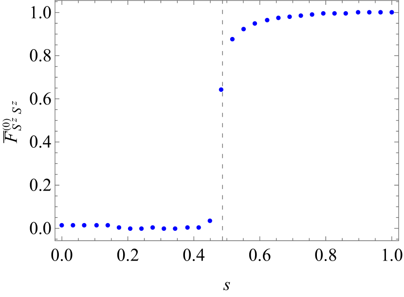
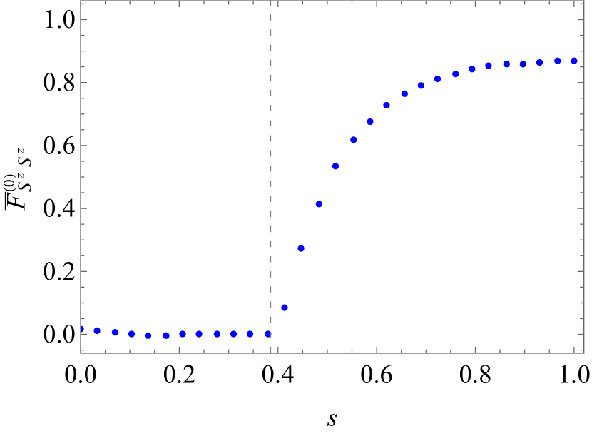
Naively, the fact that $\bar{F}^{(0)}_{X_{1}X_{8}}$ is initially one in the QP phase, and zero in the F phase, seem to suggest that the F phase is chaotic, but this is not correct. In fact, time-averaging OTOCs of the form $\bar{F}^{(0)}_{Z_{i}Z_{j}}$ start at zero in the QP phase, and approach one in the F phase. See Fig. 8(a). That means that the value that $\bar{F}^{(0)}_{VW}$ takes in each phase depends on the operators $V$ and $W$ in the corresponding OTOC. We understand this operator dependence of $\bar{F}^{(0)}_{VW}$ as due to the absence of scrambling in the ground state OTOCs. As we will see in the next section, the system under consideration displays some degree of scrambling at finite temperature, which makes thermal OTOCs to oscillate around zero at late-times in both phases. However, as we reduce the temperature, the physics is dominated by the ground state, and the behavior of $\bar{F}^{(0)}_{Z_{i}Z_{j}}$ and $\bar{F}^{(0)}_{X_{i}X_{j}}$ as a function of $s$ starts to mimic the behavior of the magnetizations $m_{z}$ and $m_{x}$, respectively.

3.3 Thermal OTOCs

We now consider thermal OTOCs to study thermal effects and the relation to chaos. Similarly to the ground state OTOCs, we first study the time-averaging thermal OTOC

$$\bar{F}_{S^{x}S^{x}}^{\beta}\equiv\lim_{T\rightarrow\infty}\frac{1}{T}\int_{0}^{T}F_{S^{x}S^{x}}^{\beta}(t)dt\,,$$ (3.7)

where

$$F_{S^{x}S^{x}}^{\beta}(t)\equiv\langle F_{S^{x}S^{x}}(t)\rangle_{\beta}\equiv\frac{\text{Tr}\left[e^{-\beta H}F_{S^{x}S^{x}}(t)\right]}{\text{Tr}\left[e^{-\beta H}\right]}\,,$$ (3.8)

with the inverse temperature $\beta$.

Fig. 7 shows that the time-averaging thermal OTOC $\bar{F}_{S^{x}S^{x}}^{\beta}$ can successfully diagnose the phase transition at small temperatures as expected. In high temperature regimes, $\bar{F}_{S^{x}S^{x}}^{\beta}$ vanishes in both phases.

(a) $p=11,\lambda=1.0$

(b) $p=5,\lambda=0.2$

Figure 7: Time average of the thermal OTOC, $\bar{F}_{S^{x}S^{x}}^{\beta}$ versus the annealing parameter $s$. The transition points for each case are indicated by vertical lines. We set $N$ = 11. $\beta$ is the inverse temperature.

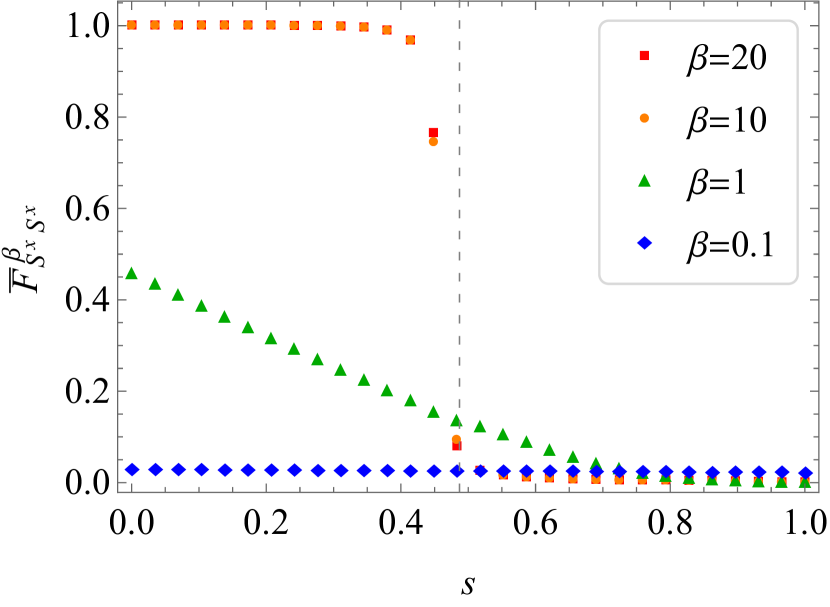
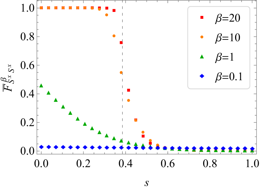
At small temperatures, thermal OTOCs are dominated by a contribution coming from the ground state, and contributions from higher excited states are exponentially suppressed. In fact, if $\mathcal{F}(t)=W(t)V(0)W(t)V(0)$, we can write

$$\langle\mathcal{F}(t)\rangle_{\beta}=\frac{\text{Tr}\left[e^{-\beta H}\mathcal{F}(t)\right]}{\text{Tr}\left[e^{-\beta H}\right]}=\frac{\sum_{n=0}^{\infty}e^{-\beta E_{n}}\langle n|\mathcal{F}(t)|n\rangle}{\sum_{n=0}^{\infty}e^{-\beta E_{n}}}=\langle 0|\mathcal{F}(t)|0\rangle+\sum_{n=1}^{\infty}\mathcal{O}\left(e^{-\beta(E_{n}-E_{0})}\right)\,,$$ (3.9)

where $|n\rangle$ denotes the state with energy $E_{n}$, with $E_{0}$ being the ground state energy. From (3.9) we see that corrections from excited states are all very small as long as the temperature is much smaller than the difference in energy between the ground state and the first excited state, i.e., $\beta(E_{1}-E_{0})>>1$. Therefore, at small temperatures, the thermal OTOC is roughly the same as the ground state OTOC, and that is why it can also diagnose phase transitions. For a more details about the relation between ground state OTOCs and phase transitions, we refer to [12].

Next, to have a clear understanding of the scrambling properties of our model, we also consider thermal OTOCs of the form, without time averaging,

$$F_{Z_{i}Z_{j}}^{\beta}(t)=\frac{\text{Tr}\,[e^{-\beta H}Z_{i}(t)Z_{j}(0)Z_{i}(t)Z_{j}(0)]}{\text{Tr}[e^{-\beta H}]}\,,$$ (3.10)

where $\beta$ is the inverse temperature and $H$ is given by (2.6). Fig. 8 shows the time dependence of $F_{Z_{1}Z_{1}}^{\beta}$ for the system in the QP phase ($s=0.2$, red curves), and for the system in the F phase ($s=0.8$, blue curves). In Fig. 8(a), we consider a very small temperature by setting $\beta=100$. In this case, the thermal OTOC oscillates around a constant value which is close to one (zero) in the QP (F) phase. In Fig. 8(b), we show the results at infinite temperature ($\beta=0$). In this case, the thermal OTOC oscillates around zero in both phases.

In chaotic systems, thermal OTOCs are expected to approach zero at late times. In our case, thermal OTOCs computed at infinite temperature ($\beta=0$) display an oscillatory behavior that persists at very large times, oscillating around zero and taking values that roughly range between -1 and 1. See Fig. 8(b). The oscillatory behavior around zero is present in both phases of the annealing process, and it happens independently of the operator considered in the OTOC. This should be contrasted with the non-universal behavior of ground state OTOCs $F_{VW}^{(0)}(t)$, which oscillate around a constant value that depends both on the phase and on the operators $V$ and $W$.

(a) Small temperature ($\beta=100$)

(b) Infinite temperature ($\beta=0$)

Figure 8: Time dependence of $F_{Z_{i}Z_{j}}^{\beta}$ for $N=11$, $p=5$ and $\lambda=0.2$. The red curves are for $s=0.2$ (QP phase) and the blue curves are for $s=0.8$ (F phase).

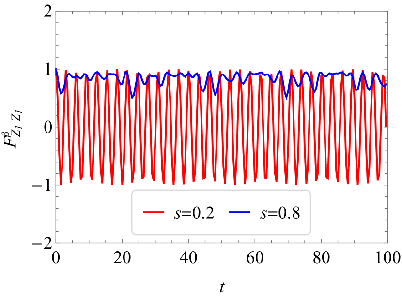
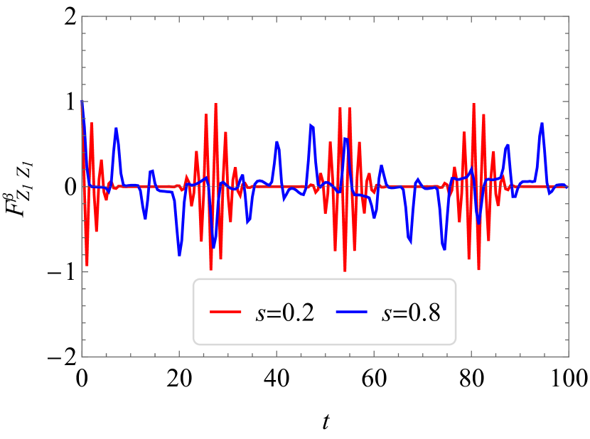
We interpret the fact that all thermal OTOCs oscillate around zero at high temperatures as some sort of weak chaotic behavior of the model (2.6). The adjective weak is because the thermal OTOC do not vanish at late-time, but only oscillates around zero. We believe this characterizes a weak chaotic behavior that takes place in relatively simple systems at finite temperature. We provide a more detailed discussion about the idea of weak scrambling in Appendix A.

4 Level Spacing Statistics

The statistics of the spacing between consecutive energy eigenvalues (level spacing) differs significantly depending on whether we consider chaotic or integrable systems. In chaotic systems, the level spacing statistics obeys a Wigner-Dyson distribution [9], while in integrable systems it follows an Poisson distribution [10, 11]. The above statement holds for a properly normalized spectrum, in which the influence of model-dependent density of states is removed by normalizing the level spacing by the local density of states. A properly normalized spectrum is said to be unfolded. Moreover, if the Hamiltonian has symmetries, one needs to block-diagonalize it according the corresponding to conserved charges, and perform the unfolding for each block, because the eigenvalues of different blocks are uncorrelated.

The Hamiltonian (2.6) conserves the total spin operator ${\bf S}^{2}=(S^{x})^{2}+(S^{y})^{2}+(S^{z})^{2}$, where $S^{x}=\frac{1}{2}\sum_{i=1}^{N}\sigma^{x}_{i}$, and so on. We will be interested in the sector with maximal total spin, in which $S=N/2$, where $S$ is the angular momentum quantum number that gives the eigenvalues of the total spin operator, i.e., ${\bf S}^{2}=S(S+1)$. The reason for that choice is because at the beginning of the annealing process, when $s=0$, the ground state of $H_{I}$ has maximal total spin. Since the total spin is conserved during the annealing process, we can restrict our analysis to this subspace.

We use the total-spin basis

$${\bf S}^{2}|S,M\rangle =S(S+1)|S,M\rangle\,,$$ (4.1)

$$S^{z}|S,M\rangle =M|S,M\rangle\,,$$ (4.2)

and, following [27], we label the states as

$$|w\rangle:=|S=N/2,M=N/2-w\rangle\,,$$ (4.3)

where $w=0,1,2,...,N$. In this subspace, the matrix elements of the Hamiltonin $[H]_{\omega,\omega^{\prime}}:=\langle\omega|H(s,\lambda)|\omega\rangle$ can be written as

$$[H]_{w,\,w} =s\left[-\lambda N\left(1-\frac{2w}{N}\right)^{p}+(1-\lambda)\left(2w-\frac{2w^{2}}{N}+1\right)\right]\,,$$ (4.4)

$$[H]_{w+1,\,w} =[H]_{w,\,w+1}=-(1-s)\sqrt{(N-w)(w+1)}\,,$$ (4.5)

$$[H]_{w+2,\,w} =[H]_{w,\,w+2}=\frac{1}{N}s(1-\lambda)\sqrt{(w+1)(w+2)(N-w)(N-w-1)}\,,$$ (4.6)

and all other elements are zero.

Here, we study the so called $r$-parameter statistics, introduced in [44]. Given a sorted spectrum $\{E_{n}\}$ and the corresponding level spacing, $s_{n}=E_{n+1}-E_{n}$, the $r$-parameter is defined by

$$r_{n}=\frac{\min\{s_{n},s_{n-1}\}}{\max\{s_{n},s_{n-1}\}}\,.$$ (4.7)

This quantity is independent of the local density of states and so it does not require unfolding. We are interested in the average $r$-parameter,

$$\tilde{r}\equiv\frac{1}{N-2}\sum_{n=2}^{N-1}r_{n}\,,$$ (4.8)

because it takes some simple benchmark values in the case of chaotic systems. For example, $\tilde{r}_{\text{GOE}}\approx 0.53590$, $\tilde{r}_{\text{GUE}}\approx 0.60266$, and $\tilde{r}_{\text{GSE}}\approx 0.67617$, for random matrices of the Gaussian Orthogonal Ensemble (GOE), Gaussian Unitary Ensemble (GUE) and Gaussian Simpletic Ensemble (GSE), respectively.. If the dynamics of a given systems is chaotic, one expects the $r$-parameter statistics to be described by random matrix theory, and $\tilde{r}$ to take one of the above-mentioned reference values. For integrable systems, one generally expects the statistics of the ratio of consecutive level spacing to be described by a Poisson distribution. In this case, $\tilde{r}_{\text{Poisson}}=0.38624$. Thus, the average $r$-parameter, $\tilde{r}$, diagnoses the chaotic behavior of the system, or the absence of it.

(a) $p=5,\lambda=1.0$

(b) $p=5,\lambda=0.2$

Figure 9: $s$ dependence of the average $r$-parameter ($\tilde{r}$) for the sector with maximal total spin. We set $N=100$. The red, purple, blue, and black horizontal lines correspond to the value of $\tilde{r}$ for GSE, GUE, GOE, and Poisson distributions. The transition values of $s$ are indicated by a vertical black dashed line. These values agree with our OTOC computation, for example, Fig. 4.

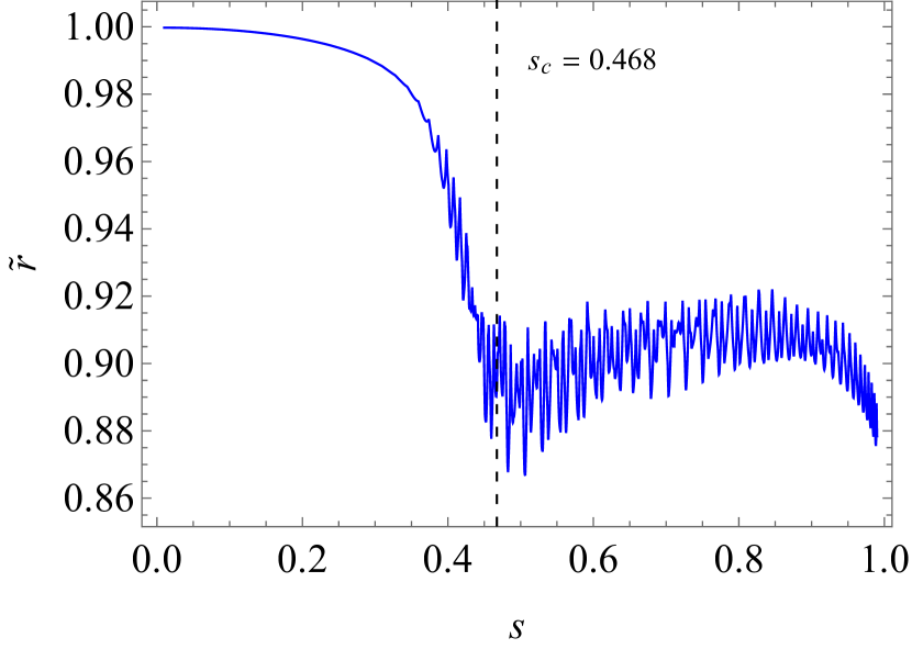
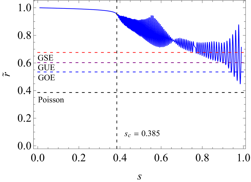
Fig. 9 exhibits $\tilde{r}$ for the maximal spin sector of the Hamiltonain (2.6). For small values of $s$, $\tilde{r}$ is close to one. As we increase $s$, the average $r$-parameter decreases slightly, and it starts to oscillate around the phase transition point. For the anti-ferromagnetic interactions at $\lambda=0.2$ (Fig. 9(a)) one can precisely find out the phase transition value of $s$, which agree with our OTOC result in Fig. 4(b). After the phase transition, in the F phase, $\tilde{r}$ oscillates wildly as we increase $s$, taking values that correspond to chaotic behavior for some specific $s$. In the case with no anti-ferromagnetic interactions at $\lambda=1$ (Fig. 9(a)), one can also estimate the phase transition value of $s$, which also agree with our OTOC result in Fig. 4(a), although in this case the phase transition point is less sharp. Moreover, in the F phase, $\tilde{r}$ oscillates around some constant value which is far away from any reference value for $\tilde{r}$. Thus, in general, our system is not chaotic.

It is interesting to question whether the behavior of $\tilde{r}$ versus $s$ can indicate the order of the phase transition. Our result suggests that it may be the case in the sense of the local average value of $\tilde{r}$ over $s$, $\tilde{r}_{\text{avg}}$, defined as

$$\tilde{r}_{\text{avg}}(s)=\frac{1}{\Delta s}\int_{s-\Delta s/2}^{s+\Delta s/2}ds^{\prime}\,\tilde{r}(s^{\prime})\,,$$ (4.9)

where $\Delta s$ is the range of the interval in $s$ that we use to compute the local average. For the second order phase transition, Fig. 9(b), the local average $\tilde{r}_{\text{avg}}(s)$ changes smoothly at the transition point, while for the first order transition, it changes abruptly Fig. 9(a).

5 Reverse Annealing and OTOCs

In this section, we study a relation between reverse annealing and OTOCs. Reverse annealing is a way to find a better classical solution than a given initial solution by starting from an appropriate classical state and gradually increasing and then decreasing the transverse magnetic field [26]. The current D-Wave quantum annealer implements reverse annealing and the performance has been studied for various cases [46, 47, 48]. Some studies on the efficiency of reverse annealing are provided theoretically [49] and numerically [50], where it is shown that, at least for the $p$-spin model, reverse annealing can turn first-order phase transition into second-order phase transition by choosing an appropriate process.

The Hamiltonian of reverse annealing we will consider is

$$H(s,\lambda)=sH_{T}+(1-s)(1-\lambda)H_{\text{init}}+\Gamma(1-s)\lambda H_{I}\,,$$ (5.1)

where $s,\lambda$ both take values in $[0,1]$ and $H_{T}$ is the Hamiltonian of the $p$-spin model (2.3). $\Gamma$ tunes the strength of the transverse magnetic field $H_{I}$ (2.2). $H_{\text{init}}$ is the initialization term

$$H_{\text{init}}=-\sum_{i=1}^{N}\epsilon_{i}Z_{i}\,,$$ (5.2)

which is $H(0,0)$ and $\epsilon_{i}\in\{-1,1\}$ is the $i$th component of the given classical initial state. Due to the high spatial symmetry of the $p$-spin model, without loss of generality we can assign $\epsilon_{i}$ as

$$\epsilon_{i}=\begin{cases}+1&\text{for~{}}i\leq N-n\,,\\ -1&\text{for~{}}i>N-n\,,\end{cases}$$ (5.3)

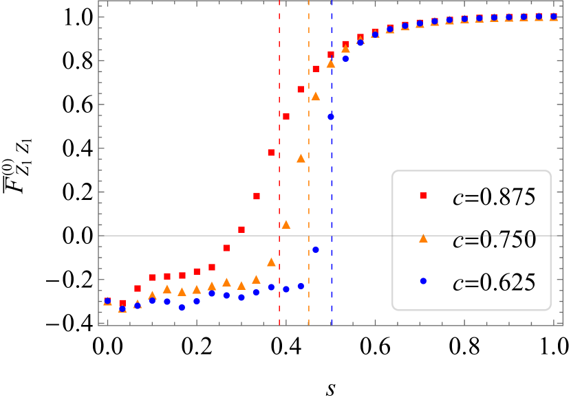
where $n\in\{0,1,\cdots,N\}$. The system may be characterized by a parameter $c=1-\frac{n}{N}\in[0,1]$, which is the probability for $\epsilon_{i}$ to be $+1$. The initial magnetization is $2c-1$. A large $c$ implies the solution is close to the ground state of $H_{T}$. According to [50], the $p$-spin model experiences phase transitions by reverse annealing. We will show that the phase transitions can be detected also by OTOCs.

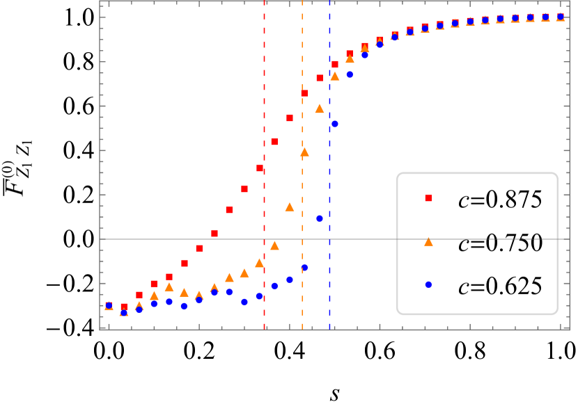
In Fig. 10 we present the time averaged OTOCs of the form $\bar{F}_{Z_{i}Z_{i}}^{(0)}$ as an example. We have confirmed that other choices of operators show the same properties. $\bar{F}_{Z_{i}Z_{i}}^{(0)}$ grows around the dotted lines corresponding to the transition points obtained by computing the free energy following [50]. This confirms that OTOCs can diagnose the phase transition. The smaller $c$ becomes, the larger the transition $s$ becomes. The bigger $\Gamma$ becomes, the bigger the transition points $s$ becomes. All these properties are also consistent with [50]. Furthermore, the curves for $c=0.625$ (blue circles) suggest a first order phase transition, while the curves for $c=0.875$ (red squares) suggest a second order phase transition. The results for $c=0.750$ depend on the value of $\Gamma$. For $\Gamma=1$, they suggest a first order phase transition, while for $\Gamma=5$ they suggest a second order phase transition. These are also consistent with [50], and provide more evidences that time-averaging OTOCs can diagnose also the order of phase transitions. The time-averaging OTOCs may play the role of an order parameter.

(a) $p=5,\Gamma=1$

(b) $p=11,\Gamma=1$

(c) $p=5,\Gamma=5$

(d) $p=11,\Gamma=5$

Figure 10: $\bar{F}_{Z_{i}Z_{i}}^{(0)}$ versus $s$ during the reverse annealing process for $N=8$ and $\lambda=0.2$. The left panel show the results for $p=5$, while the right panel show the results for $p=11$. We set $\Gamma=1$ in the first row, and $\Gamma=5$ in the second row.

6 Conclusions and Future Directions

In this work, we have studied quantum phase transitions associated with quantum annealing and reverse quantum annealing for the ferromagnetic $p$-spin model from the point of view of quantum chaos. More specifically, we have shown that time-averaging OTOCs and the $r$-parameter statistics, which are usually used to diagnose quantum chaos, can also be used to diagnose quantum phase transitions.

In the case of quantum annealing (QA), the system’s ground state is initially in a quantum paramagnetic (QP) phase ($s=0$). As we increase the value of $s$, the system displays a quantum phase transition to a ferromagnetic (F) phase. We observe that the time-averaging OTOC takes an approximately constant value which is different in each phase. The late-time average value of OTOCs of the form $F_{Z_{i}Z_{j}}^{(0)}=\langle Z_{i}(0)Z_{j}(t)Z_{i}(0)Z_{j}(t)\rangle$ vanishes in the QP phase, and it takes a non-zero value in the F phase. In contrast, in the case of OTOCs of the form $F_{X_{i}X_{j}}^{(0)}=\langle X_{i}(0)X_{j}(t)X_{i}(0)X_{j}(t)\rangle$, the late-time average value is non-zero in the QP phase and zero in the F phase. In both cases, despite having different values in each phase depending on the choice of operator in the OTOC, the time-averaging OTOC sharply diagnoses the quantum phase transitions. Time-averaging OTOCs made out of non-local operators, $\bar{F}^{(0)}_{S^{z}S^{z}}$ and $\bar{F}^{(0)}_{S^{x}S^{x}}$, show a qualitatively similar behavior to the local operators $\bar{F}^{(0)}_{Z_{i}Z_{j}}$ and $\bar{F}^{(0)}_{X_{i}X_{j}}$, respectively.

The operator-dependence of $\bar{F}^{(0)}_{VW}$ occurs because we are considering ground state OTOCs. The ground-state OTOCs is essentially controlled by the properties of the ground state and do not reflect any chaotic property of ferromagnetic $p$-spin model. To access the chaotic properties of the model, we need to consider thermal OTOCs at temperatures which are sufficiently larger than the ground state energy, in such a way that the OTOC receives contributions from excited states. In those cases, however, the thermal fluctuations washes out the special properties of the ground state, and the OTOCs are no longer useful in diagnosing phase transition. This can be seen in Fig. 7, which shows that the time-averaging thermal OTOCs vanish in both phases at high temperature.

The thermal OTOCs oscillate with time wildly around zero at late times, taking values which range roughly from -1 to 1. See Fig. 8. We think this oscillatory behavior reflects two effects: finite-size effects and some sort of weak chaotic behavior. Finite-size effects account for the fact that OTOCs do not vanish at late-times in systems whose size is not very large. In fact, it was shown in [40] that for energy-conserving system the late-time value of OTOCs scale as an inverse polynomial in the system size. Since our calculation of thermal OTOCs were done for $N\sim 11$, we expect finite-size effects in our results. The second effect, which we call weak scrambling, is based on the idea that, if the system is not strongly chaotic, or even if it is integrable, the thermal OTOC (for spatially separated operators) will not vanish at late times, but it will rather oscillate around zero, with the size of the oscillation being smaller for systems which are more chaotic. We give more evidence for these ideas in Appendix A using the chaotic Ising model. Similar ideas are also explored in [52].

From the above-mentioned results, we could confirm that time-averaging OTOCs provide useful order parameters to detect quantum phase transition, as suggested in [30]. Interestingly, time-averaging OTOCs not only diagnose the phase transition, but they can also distinguish first-order and second order phase transitions. In the case of first-(second-) order phase transitions, the time averaging OTOCs display a discontinuous (continuous) behavior at the quantum transition point, just like ordinary order parameters. This suggests that time-averaging OTOCs might be useful in detecting phase transitions when the rigorous order parameter is unknown.

The effectiveness of ground state OTOCs in detecting quantum phase transitions motivated us to question if we could also diagnose phase transitions using other probes of quantum chaos. In order to do that, we have studied how the average $r$-parameter behaves during the quantum annealing process. Fig. 9 shows that the average $r$-parameter clearly changes behavior around the quantum transition point, with the phase transition being more sharp in the case with anti-ferromagnetic interactions ($\lambda=0.2$). When $\lambda=1$, the average $r$-parameter, $\tilde{r}$, never takes any reference value characterizing random matrix behavior or integrability. In contrast, for $\lambda=0.2$, the curves of $\tilde{r}$ versus $s$ display large oscillations in the ferromagnetic phase, taking values that correspond to chaotic behavior at some specific $s$. However, we checked that the corresponding level spacing distributions are different from Poisson or random matrix distributions, although they might have some vague resemblance. Interestingly, the local average of $\tilde{r}$ also can distinguish first and second order phase transition like OTOCs. Since we have studied the $r$-parameter statistics in the maximal spin sector, and the ground state of the system belongs to this sector, it is natural that it can detect the ground state physics associated to the phase transition.

In the case of reverse QA, the $p$-model also displays quantum phase transitions, as shown in [50]. Similarly to the QA case, the time-averaging OTOC also can diagnose the quantum phase transition and its order. There is a quantitative difference from the QA case. In the beginning of the reverse annealing schedule, at $s=0$, the system already displays a non-zero value of $\bar{F}_{Z_{i}Z_{i}}^{(0)}$, which then increases as we increase the values of $s$.

Finally, we make a comment about the presence of the anti-ferromagnetic interaction term, $H_{AF}$, which makes the Hamiltonian non-stoquastic and turns first-order phase transitions into second-order ones during the quantum annealing process. From the analysis of the level spacing statistic we observe that this term makes the dynamics richer in the ferromagnetic phase. In particular, for some values of $s$, the system displays some degree of level repulsion, which is typical of chaotic systems. This suggests a connection between chaos and the order of the phase transitions. In particular, it seems that the presence of chaos in the ground state sector may turn first order phase transitions into second order ones. It would be interesting to further investigate this possibility.

Appendix A Chaotic/Integrable Transition in the Ising Spin Chain

In this section we review the time-behavior of OTOCs for the Ising model with transverse and magnetic fields,

$$H=-\sum_{i=1}^{L-1}Z_{i}Z_{i+1}-\sum_{i=1}^{L}\left(h_{x}X_{i}+h_{z}Z_{i}\right)\,,$$ (A.1)

where we chose open boundary conditions. The Hamiltonian (A.1) is known to display chaotic behavior when $(h_{x},h_{z})=(-1.05,0.5)$ [53]. The system is integrable if either $h_{x}$ or $h_{z}$ vanish.

We will be interested in the behavior of thermal OTOCs of the form

$$F_{Z_{i}Z_{j}}(t)=\langle Z_{i}(0)Z_{j}(t)Z_{i}(0)Z_{j}(t)\rangle\,,$$ (A.2)

where the expectation value is taken in a thermal state.

(a) $\beta=0$

(b) $\beta=50$

Figure 11: Thermal OTOCs, $F_{Z_{i}Z_{j}}(t)=\langle Z_{i}(0)Z_{j}(t)Z_{i}(0)Z_{j}(t)\rangle$, for the Ising model with longitudinal and transverse magnetic fields ($L=8$).

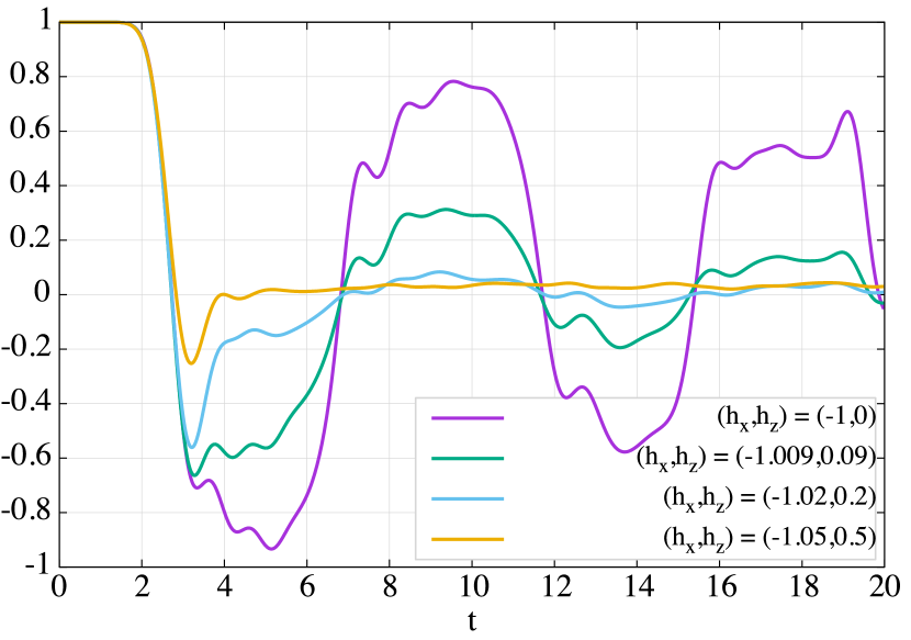
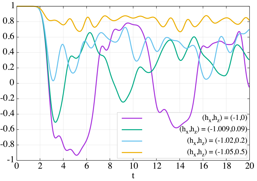
In Fig. 11 we study the behavior of OTOCs across the integrable/chaotic transition that takes place as we change the parameters from the integrable point $(h_{x},h_{z})=(-1,0)$ to the strongly chaotic point $(h_{x},h_{z})=(-1.05,0.5)$.

Let us first discuss the infinite-temperature results, which are shown in Fig. 11(a). At the strongly chaotic point $(h_{x},h_{z})=(-1.05,0.5)$, the OTOC vanishes at late times, which is a signal of scrambling . As we move away from the strongly chaotic point, the OTOC starts to oscillate around zero, and the amplitude of the oscillations increase as we approach the integrable point. We understand this behavior as a manifestation of weak scrambling, in which the OTOCs do not vanish at late times, but rather oscillates around zero, with the amplitude of the oscillations being smaller for more chaotic cases.

The behavior of the OTOCs change as we reduce the system’s temperature. Fig. 11(b) shows the results for $\beta=50$, which are almost same as the corresponding ground state OTOCs. Interestingly, the OTOCs at the integrable point $(h_{x},h_{z})=(-1,0)$ do not seem to depend on the temperature. For all other values of $(h_{x},h_{z})$, the late-time value of the OTOC does not approach zero at late times. Instead, it oscillates around some constant value that depends on $(h_{x},h_{z})$. This shows that the OTOC no longer displays universal behavior at small temperatures, being actually controlled by the ground state physics. Note that this happens even at the strong chaotic point $(h_{x},h_{z})=(-1.05,0.5)$. We understand this phenomenon as an absence of scrambling at low temperatures.

The observed behavior of the OTOCs for the quantum annealing Hamiltonian (2.6) are qualitatively similar to the ones obtained for the Ising model when we move slightly away from the integrable point, e.g. $(h_{x},h_{z})=(-1.02,.02)$. In both cases the thermal OTOCs (for sufficiently high temperatures) oscillate around zero taking some $\mathcal{O}(1)$ values. This suggests that the system described by the Hamiltonian (2.6) is close to be integrable.

References

- [1] A. Larkin and Y. N. Ovchinnikov, Quasiclassical method in the theory of superconductivity, Sov Phys JETP 28 (1969) 1200.
- [2] A. Kitaev, “Hidden correlations in the hawking radiation and thermal noise.”
- [3] J. Maldacena, S. H. Shenker and D. Stanford, A bound on chaos, JHEP 08 (2016) 106 [1503.01409].
- [4] V. Jahnke, Recent developments in the holographic description of quantum chaos, Adv. High Energy Phys. 2019 (2019) 9632708 [1811.06949].
- [5] B. Yoshida and N. Y. Yao, Disentangling Scrambling and Decoherence via Quantum Teleportation, Physical Review X 9 (2019) 011006 [1803.10772].
- [6] M. Gärttner, J. G. Bohnet, A. Safavi-Naini, M. L. Wall, J. J. Bollinger and A. M. Rey, Measuring out-of-time-order correlations and multiple quantum spectra in a trapped-ion quantum magnet, Nature Physics 13 (2017) 781 [1608.08938].
- [7] J. Li, R. Fan, H. Wang, B. Ye, B. Zeng, H. Zhai et al., Measuring Out-of-Time-Order Correlators on a Nuclear Magnetic Resonance Quantum Simulator, Physical Review X 7 (2017) 031011 [1609.01246].
- [8] R. J. Lewis-Swan, A. Safavi-Naini, J. J. Bollinger and A. M. Rey, Unifying scrambling, thermalization and entanglement through measurement of fidelity out-of-time-order correlators in the Dicke model, Nature Communications 10 (2019) 1581 [1808.07134].
- [9] O. Bohigas, M. J. Giannoni and C. Schmit, Characterization of chaotic quantum spectra and universality of level fluctuation laws, Phys. Rev. Lett. 52 (1984) 1.
- [10] B. M. Victor, T. M. and Z. J. Michael, Level clustering in the regular spectrum, Proc. R. Soc. Lond. A 356 (1977) .
- [11] M. V. Berry, Quantizing a classically ergodic system: Sinai’s billiard and the kkr method, Annals of Physics 131 (1981) 163.
- [12] C. B. Dağ, K. Sun and L. M. Duan, Detection of Quantum Phases via Out-of-Time-Order Correlators, Phys. Rev. Lett. 123 (2019) 140602 [1902.05041].
- [13] Z.-H. Sun, J.-Q. Cai, Q.-C. Tang, Y. Hu and H. Fan, Out-of-time-order correlators and quantum phase transitions in the rabi and dicke models, Annalen der Physik n/a 1900270 [https://onlinelibrary.wiley.com/doi/pdf/10.1002/andp.201900270].
- [14] Q. Wang and F. Pérez-Bernal, Probing excited-state quantum phase transition in a quantum many body system via out-of-time-ordered correlator, arXiv e-prints (2018) arXiv:1812.01920 [1812.01920].
- [15] A. M. García-García, T. Nosaka, D. Rosa and J. J. Verbaarschot, Quantum chaos transition in a two-site Sachdev-Ye-Kitaev model dual to an eternal traversable wormhole, Phys. Rev. D 100 (2019) 026002 [1901.06031].
- [16] T. Nosaka and T. Numasawa, Quantum chaos, thermodynamics and black hole microstates in the mass deformed syk model, 2020.
- [17] T. Nosaka and T. Numasawa, Chaos exponents of syk traversable wormholes, 2020.
- [18] M. Vojta, Quantum phase transitions, Reports on Progress in Physics 66 (2003) 2069–2110.
- [19] T. Kadowaki and H. Nishimori, Quantum annealing in the transverse ising model, Phys. Rev. E 58 (1998) 5355.
- [20] E. Farhi, J. Goldstone, S. Gutmann and M. Sipser, Quantum Computation by Adiabatic Evolution, ArXiv e-prints (2000) quant [quant-ph/0001106].
- [21] B. Damski and M. M. Rams, Exact results for fidelity susceptibility of the quantum ising model: the interplay between parity, system size, and magnetic field, Journal of Physics A: Mathematical and Theoretical 47 (2013) 025303.
- [22] S. Dusuel and J. Vidal, Continuous unitary transformations and finite-size scaling exponents in the lipkin-meshkov-glick model, Phys. Rev. B 71 (2005) 224420.
- [23] P. Pfeuty, The one-dimensional ising model with a transverse field, Annals of Physics 57 (1970) 79 .
- [24] C. R. Laumann, R. Moessner, A. Scardicchio and S. L. Sondhi, Quantum adiabatic algorithm and scaling of gaps at first-order quantum phase transitions, Phys. Rev. Lett. 109 (2012) 030502.
- [25] J. Tsuda, Y. Yamanaka and H. Nishimori, Energy gap at first-order quantum phase transitions: An anomalous case, Journal of the Physical Society of Japan 82 (2013) 114004 [https://doi.org/10.7566/JPSJ.82.114004].
- [26] A. Perdomo-Ortiz, S. E. Venegas-Andraca and A. Aspuru-Guzik, A study of heuristic guesses for adiabatic quantum computation, Quantum Information Processing 10 (2011) 33.
- [27] Y. Susa, J. F. Jadebeck and H. Nishimori, Relation between quantum fluctuations and the performance enhancement of quantum annealing in a nonstoquastic hamiltonian, Phys. Rev. A 95 (2017) 042321.
- [28] G. Passarelli, K.-W. Yip, D. A. Lidar, H. Nishimori and P. Lucignano, Reverse quantum annealing of the -spin model with relaxation, arXiv e-prints (2019) arXiv:1911.07186 [1911.07186].
- [29] M. Filippone, S. Dusuel and J. Vidal, Quantum phase transitions in fully connected spin models: An entanglement perspective, Phys. Rev. A 83 (2011) 022327 [1101.3654].
- [30] M. Heyl, F. Pollmann and B. Dóra, Detecting equilibrium and dynamical quantum phase transitions in ising chains via out-of-time-ordered correlators, Physical Review Letters 121 (2018) .
- [31] H. Shen, P. Zhang, R. Fan and H. Zhai, Out-of-time-order correlation at a quantum phase transition, Phys. Rev. B 96 (2017) 054503 [1608.02438].
- [32] C. B. Dağ, K. Sun and L.-M. Duan, Detection of quantum phases via out-of-time-order correlators, Phys. Rev. Lett. 123 (2019) 140602.
- [33] R. K. Shukla, G. K. Naik and S. K. Mishra, Out-of-time-order correlation and detection of phase structure in floquet transverse ising spin system, 2020.
- [34] S. Bravyi, D. P. DiVincenzo, R. I. Oliveira and B. M. Terhal, The Complexity of Stoquastic Local Hamiltonian Problems, arXiv e-prints (2006) quant [quant-ph/0606140].
- [35] Y. Seki and H. Nishimori, Quantum annealing with antiferromagnetic fluctuations, Phys. Rev. E 85 (2012) 051112 [1203.2418].
- [36] T. Jörg, F. Krzakala, J. Kurchan, A. C. Maggs and J. Pujos, Energy gaps in quantum first-order mean-field–like transitions: The problems that quantum annealing cannot solve, EPL (Europhysics Letters) 89 (2010) 40004.
- [37] K. Ikeda, Universal computation with quantum fields, Quantum Information Processing 19 (2020) 331.
- [38] Y. Ahn, V. Jahnke, H.-S. Jeong and K.-Y. Kim, Scrambling in Hyperbolic Black Holes: shock waves and pole-skipping, JHEP 10 (2019) 257 [1907.08030].
- [39] V. Jahnke, K.-Y. Kim and J. Yoon, On the Chaos Bound in Rotating Black Holes, JHEP 05 (2019) 037 [1903.09086].
- [40] Y. Huang, F. G. S. L. Brandão and Y.-L. Zhang, Finite-size scaling of out-of-time-ordered correlators at late times, Phys. Rev. Lett. 123 (2019) 010601 [1705.07597].
- [41] V. Khemani, D. A. Huse and A. Nahum, Velocity-dependent Lyapunov exponents in many-body quantum, semiclassical, and classical chaos, Phys. Rev. B98 (2018) 144304 [1803.05902].
- [42] B. Craps, M. D. Clerck, D. Janssens, V. Luyten and C. Rabideau, Lyapunov growth in quantum spin chains, 1908.08059.
- [43] H. Gharibyan, M. Hanada, B. Swingle and M. Tezuka, Quantum Lyapunov Spectrum, JHEP 04 (2019) 082 [1809.01671].
- [44] V. Oganesyan and D. A. Huse, Localization of interacting fermions at high temperature, Physical Review B 75 (2007) .
- [45] Y. Y. Atas, E. Bogomolny, O. Giraud and G. Roux, Distribution of the ratio of consecutive level spacings in random matrix ensembles, Physical Review Letters 110 (2013) .
- [46] K. Ikeda, Y. Nakamura and T. S. Humble, Application of quantum annealing to nurse scheduling problem, Scientific Reports 9 (2019) 12837.
- [47] D. Venturelli and A. Kondratyev, Reverse quantum annealing approach to portfolio optimization problems, Quantum Machine Intelligence 1 (2019) 17.
- [48] A. D. King, J. Carrasquilla, J. Raymond, I. Ozfidan, E. Andriyash, A. Berkley et al., Observation of topological phenomena in a programmable lattice of 1,800 qubits, Nature 560 (2018) 456.
- [49] M. Ohkuwa, H. Nishimori and D. A. Lidar, Reverse annealing for the fully connected -spin model, Phys. Rev. A 98 (2018) 022314.
- [50] Y. Yamashiro, M. Ohkuwa, H. Nishimori and D. A. Lidar, Dynamics of reverse annealing for the fully connected -spin model, Phys. Rev. A 100 (2019) 052321.
- [51] X. Nie, B.-B. Wei, X. Chen, Z. Zhang, X. Zhao, C. Qiu et al., Experimental observation of equilibrium and dynamical quantum phase transitions via out-of-time-ordered correlators, 2019.
- [52] E. M. Fortes, I. García-Mata, R. A. Jalabert and D. A. Wisniacki, Gauging classical and quantum integrability through out-of-time-ordered correlators, Physical Review E 100 (2019) .
- [53] M. C. Bañuls, J. I. Cirac and M. B. Hastings, Strong and Weak Thermalization of Infinite Nonintegrable Quantum Systems, Phys. Rev. Lett. 106 (2011) 050405 [1007.3957].