Causal Inference in the Presence of Interference in Sponsored Search Advertising

Abstract

In classical causal inference, inferring cause-effect relations from data relies on the assumption that units are independent and identically distributed. This assumption is violated in settings where units are related through a network of dependencies. An example of such a setting is ad placement in sponsored search advertising, where the clickability of a particular ad is potentially influenced by where it is placed and where other ads are placed on the search result page. In such scenarios, confounding arises due to not only the individual ad-level covariates but also the placements and covariates of other ads in the system. In this paper, we leverage the language of causal inference in the presence of interference to model interactions among the ads. Quantification of such interactions allows us to better understand the click behavior of users, which in turn impacts the revenue of the host search engine and enhances user satisfaction. We illustrate the utility of our formalization through experiments carried out on the ad placement system of the Bing search engine.

1 Introduction

In recent years, advertisers have increasingly shifted their ad expenditures online. One of the most effective platforms for online advertising is search engine result pages. Given a user query, the search engine allocates a few ad slots (e.g., above or below its organic search results) and runs an auction among advertisers who are bidding and competing for these slots. Quantifying the effectiveness of ad placement is vital not only to the experience of the user, but also revenue of the advertiser and the search engine. Click yield is a common metric used in this regard. Often, statistical models are used to predict the click behavior of users by estimating the likelihood of receiving a click in a given slot using logged data. A rich literature is devoted to click prediction in sponsored search advertising (Xiong et al., 2012; Cheng et al., 2012; Nabi-Abdolyousefi, 2015; Zhang et al., 2014; Effendi and Ali, 2017). However, a comprehensive understanding of click behavior requires causal, rather than associative, reasoning (Bottou et al., 2013; Hill et al., 2015; Zeng et al., 2019; Yin et al., 2014).

Causal inference is central to making data-driven decisions. Inferring valid cause-effect relations, even with granular data and large sample sizes, is complicated by confounding induced by common causes of observed exposures and outcomes. In classical causal inference, it is assumed that samples are independent and identically distributed (iid). However, a causal view of ad placement under the iid assumption is implausible as ads interfere with one another from the beginning of the auction until the end when clicks on impressed ads are recorded. In non-iid settings, confounding arises due to not only the individual ad-level covariates but also the exposures and covariates of other ads in the system. This is commonly referred to as interference (Hudgens and Halloran, 2008). Incorporating knowledge of interference into the statistical models used to compute rank scores for each ad can help optimize the profitability of the final layout of each search page. Moreover, a proper understanding of the interference issue in relation to causal inference directly impacts engineering of more purposeful interventions and design of more effective A/B testing for ad placement.

In this paper, we formalize the problem of interference among ads using the language of causal inference. To the best of our knowledge, this is the first attempt to analyze ads under the plausible and realistic setting of interference. Throughout the paper, we discuss mechanisms that give rise to interference in ad placement. Using graphical models, we assume a causal structure that encodes the various sources of interference. We formulate our causal questions and discuss the identification and estimation of relevant effects. Our experiments find statistically significant interference effects among ads. We further adapt the constraint-based structure learning algorithm Fast Causal Inference (Spirtes et al., 2000) to verify the soundness of our presumed causal structure and learn the underlying mechanisms that give rise to interference. Finally, we incorporate the knowledge of interference to improve the performance of the statistical models used during the course of the auction. We demonstrate this improvement in performance by running experiments that closely resemble the framework in the Genie model – an offline counterfactual policy estimation framework for optimizing Sponsored Search Marketplace in Bing ads (Bayir et al., 2019).

2 Preliminaries and Setup

In causal inference, we are interested in quantifying the cause-effect relationships between a treatment variable $A$ and an outcome $Y$ using experimental or observational data. A common setting assumes that the treatment received by one unit does not affect the outcomes of other units – this is known as the stable unit treatment value assumption or SUTVA Rubin (1980) and is informally referred to as the “no-interference” assumption. In this setting, the average causal effect (ACE) of a binary treatment $A$ on $Y$ is defined as $\textit{ACE}\coloneqq\mathbb{E}[Y(1)]-\mathbb{E}[Y(0)],$ where $Y(a)$ denotes the counterfactual/potential outcome $Y$ had treatment $A$ been assigned to $a,$ possibly contrary to the fact.

Causal inference uses assumptions in causal models to link the observed data distribution to the distribution over counterfactual random variables. A simple example of a causal model is the conditionally ignorable model which encodes three main assumptions: (i) Consistency assumes the mechanism that determines the value of the outcome does not distinguish the method by which the treatment was assigned, as long as the treatment value assigned was invariant, (ii) Conditional ignorability assumes $Y(a)\perp A\mid X,$ where $X$ acts as a set of observed confounders, such that adjusting for their influence suffices to remove all non-causal dependence between $A$ and $Y,$ and (iii) Positivity of $p(A=a\mid X=x),\forall a,x.$ Under these assumptions, $p(Y(a))$ is identified as the following function of the observed data: $\sum_{X}p(Y\mid A=a,X)\times p(X),$ known as backdoor adjustment or g-formula (Pearl, 2009; Robins, 1986). For a general identification theory of causal effects in the presence of unmeasured confounders see (Tian and Pearl, 2002; Shpitser and Pearl, 2006; Huang and Valtorta, 2006; Bhattacharya et al., 2020a). Alternative causal quantities of interest include conditional causal effects (effects within subpopulations defined by covariates)Shpitser and Pearl (2012), mediation quantities (which decompose effects into components along different mechanisms)Shpitser (2013), and the effects of decision rules in sequential settings (such as dynamic treatment regimes in personalized medicine)Nabi et al. (2018).

In this paper, we relax the implausible assumption of no-interference in ad placement. Interference among ads across different pageviews creates the most extreme scenario of full interference, as this allows for user interaction with the system over multiple time frames. Following the convention in (Sobel, 2006; Hudgens and Halloran, 2008; Tchetgen and VanderWeele, 2012; Ogburn et al., 2014), we model only interference within pageviews and restrict any cross-pageview interference among ads. In other words, we restrict the interference to spatial constraints and exclude temporal dependence across pageviews. This is known as partial interference and could be justified by the fact that pageviews are query specific and are separated by time and space. In presence of interference, the counterfactual $Y(a)$ is no longer well-defined as we need to distinguish ads by a proper indexing scheme and consider the treatment assignments of other ads simultaneously.

Suppose we have $N$ pageviews, indexed by $n=1,\ldots,N,$ with each containing $m$ impressed ads. We index the ads on each pageview by $i=1,\dots,m$ based on the order in which they appear on the page. The $i$-th ad on the $n$-th pageview is represented by the tuple $(X_{ni},A_{ni},Y_{ni}),$ where $X_{ni}$ denotes the vector that collects all the ad-specific features such as geometric features (e.g., line width, pixel height), decorative features (e.g., rating information, twitter followers), and other textual features extracted from the ad. $A_{ni}$ denotes the treatment and is predefined by the analyst. An example of a treatment is the block membership of the ad: an indicator that specifies whether the ad is placed on top of the page (Top) or bottom of the page (Bottom). Ads can also appear elsewhere such as the sidebars. In this paper, without loss of generality, we assume we only have two distinct blocks of ads on each pageview: Top and Bottom. $Y_{ni}$ denotes a binary indicator of receiving a click by the user. We denote the state space of a random variable $V$ by $\mathfrak{X}_{V}.$

Let ${\bf X}_{n}\coloneqq(X_{n1},\dots,X_{nm}),$ ${\bf A}_{n}\coloneqq(A_{n1},\dots,A_{nm}),$ and ${\bf Y}_{n}\coloneqq(Y_{n1},\dots,Y_{nm})$ collect the features, treatment assignments, and outcomes of all the ads on the $n$-th pageview, respectively. We define the counterfactual $Y_{ni}({\bf a}_{n})$ to be the click response of the $i$-th ad on the $n$-th pageview where every ad on the same pageview is relocated according to the treatment assignment rule ${\bf a}_{n},$ which is a vector of size $m$ and the $i$-th element $a_{i}$ denotes the treatment value of the $i$-th ad. This notation makes the interference among ads on the same pageview more explicit as the potential outcome of a single ad now depends on the entire treatment assignment ${\bf a}_{n},$ rather than just $a_{ni}.$ The causal effect of interventions in the presence of interference can be quantified by comparing such counterfactuals under different interventions; for instance $Y_{ni}({\bf a}_{n})$ vs $Y_{ni}({\bf a^{\prime}}_{n}),$ where ${\bf a}_{n}$ and ${\bf a^{\prime}}_{n}$ denote two plausible interventions.

In the next section, we discuss various sources that give rise to interference among ads and propose a causal graphical model that captures such interactions in a reasonable way. In what follows, we discuss various ways of quantifying the interference effect among ads and provide sufficient conditions for identification of such effects along with estimation strategies.

3 Ad Placement in the Presence of Interference

We describe ad placement in the presence of interference by a system of nonparametric structural equation models with independent errors (Pearl, 2009). The key characteristic of structural models is that they represent each variable as deterministic functions of their direct causes together with an unobserved exogenous noise term, which itself represents all causes outside of the model. Let $U$ denote a variable capturing user intention which is unknown and hidden to the analyst. Given such intent, the user types a query, denoted by $C,$ which is expressed as an unrestricted function of the intent $U$ and a noise term $\epsilon_{c},$ denoted by $f_{c}(.).$ Upon observing the query, a set of ads are selected from the inventory, then online auction is run to determine winner ads to be displayed on the page. The $i$-th displayed ad is denoted by $X_{i}.$ The relation between $X_{i}$ and $C$ is captured by an unrestricted function $f_{x_{i}}(.)$ and the perturbation term $\epsilon_{x_{i}}.$ The block allocation of $i$-th ad is denoted by $A_{i}.$ The set of all impressed ads and the allocations are denoted by $\bf X$ and $\bf A,$ respectively (we suppress the indexing of pageviews for clarity.) The information on $U,{\bf X},{\bf A},$ along with the noise term $\epsilon_{y_{i}},$ determines whether the $i$-th ad is clicked or not which is captured by $Y_{i}.$ The structural equation models are summarized as follows.

user intent $$U\ \leftarrow\ f_{u}(\epsilon_{u})$$

user query $$C\ \leftarrow\ f_{c}(U,\epsilon_{c})$$

i-th ad $$X_{i}\ \leftarrow\ f_{x_{i}}(C,\epsilon_{x_{i}})$$

i-th ad’s allocation $$A_{i}\ \leftarrow\ f_{a_{i}}({\bf X},\epsilon_{a_{i}})$$

i-th ad’s click indication $$Y_{i}\ \leftarrow\ f_{y_{i}}(U,{\bf X},{\bf A},\epsilon_{y_{i}})$$ (1)

Note that in the above equations, when allocating the $i$-th ad to Top or Bottom, we are not only considering the corresponding features of the ad itself, but also features of other ads on the page, hence the entire array of $\bf X$ is acting as causes of $A_{i}.$ Similarly, we allow for the entire vector of $\bf A$ and array of $\bf X$ to influence $Y_{i}.$ These equation capture the interference mechanism in ad placement. In the absence of interference, the above equations simplify by replacing the allocation structural equation with $A_{i}\leftarrow f_{a_{i}}(X_{i},\epsilon_{a_{i}})$ and the click indication structural equation with $Y_{i}\leftarrow f_{y_{i}}(U,X_{i},A_{i},\epsilon_{y_{i}}).$

Causal relationships are often represented by graphical causal models (Spirtes et al., 2000; Pearl, 2009). Such models generalize independence models on directed acyclic graphs (DAGs) to also encode conditional independencies on counterfactual variables (Richardson and Robins, 2013). A DAG ${\mathcal{G}}(V)$ consists of a set of nodes $V$ connected through directed edges such that there are no directed cycles. We will abbreviate ${\mathcal{G}}(V)$ as simply ${\mathcal{G}},$ when the vertex set is clear from the given context. Statistical models of a DAG ${\mathcal{G}}$ are sets of distributions that factorize as $p(V)=\prod_{V_{i}\in V}p(V_{i}\mid\operatorname{pa}_{\mathcal{G}}(V_{i}))$, where $\operatorname{pa}_{\mathcal{G}}(V_{i})$ are the parents of $V_{i}$ in ${\mathcal{G}}$. The absence of edges between variables in ${\mathcal{G}},$ relative to a complete DAG entails conditional independence facts in $p(V).$ These can be directly read off from the DAG ${\mathcal{G}}$ by the well-known d-separation criterion (Pearl, 2009). That is, for disjoint sets $X,Y,Z$, the following global Markov property holds: $(X\perp\!\!\!\perp_{\text{d-sep}}Y\mid Z)_{\mathcal{G}}\implies(X\perp\!\!\!\perp Y\mid Z)_{p(V)}.$ When the context is clear, we will simply use $X\perp\!\!\!\perp Y\mid Z$ to denote the conditional independence between $X$ and $Y$ given $Z.$ The DAG representation of the structural equations in (1) for a pageview with three impressed ads is shown in Fig. 1(a). For simplicity and to avoid cluttering the graph, we only depict the outcome of the $i$-th ad on the DAG and marginalize out all the other outcomes (since all the outcomes share the same set of parents.) The statistical model of the DAG in Fig. 1(a), assuming all outcomes are included on the DAG, can be written as, $p(U,C,{\bf X,A,Y})=p(U)\times p(C\mid U)\times\prod_{i=1}^{3}\ \big{\{}p(X_{i}\mid C)\times p(A_{i}\mid{\bf X})\times p(Y_{i}\mid U,{\bf X,A})\big{\}}.$

Figure 1: (a) DAG representation of the SEM in 1 for a pageview with three impressed ads (the independent error terms are omitted from the graph for simplicity.) (b) The corresponding SWIG where we intervene on $\bf A$ and set the block allocations $(A_{1},A_{2},A_{3})$ to $(a_{1},a_{2},a_{3}).$

As we mentioned earlier, the user intent is unmeasured. We further restrict our attention to ad-specific features and leave the query-specific features aside. In other words $U$ and $C$ are both treated as latent. We highlight this in Fig 1(a) by coloring both vertices and the relevant edges in gray. In this case, the joint distribution over observed variables ${\bf X,A,Y}$ and latent variables $U,C$ is said to be Markov relative to a hidden variable DAG. There may be infinitely many hidden variable DAGs that imply the same set of conditional independences on the observed margin, i.e., $p({\bf X,A,Y}).$ It is typical to use a single acyclic directed mixed graph that entails the same set of equality constraints as this infinite class; see Verma and Pearl (1990); Richardson et al. (2017) for more details.

3.1 Sources of Interference in Ad Placement

In order to better understand the interference behavior among ads, we need to identify the causal mechanisms that give rise to such behaviors. Looking at our causal model in Fig. 1(a), we allow for two distinct pathways through which other ads influence $Y_{i}.$ One is direct pathways such as $X_{j}\rightarrow Y_{i}$ and $A_{j}\rightarrow Y_{i}$. This type of interference is called direct interference. As an example, suppose a low quality ad (determined by various scores) is placed in the Top. The poor quality of this ad may shape the user’s opinion about the sorted search results in negative ways, preventing them from clicking on further ads. Similarly, placing a high quality ad in the Top may convince the user to return and explore more ads. Other pathways by which outcomes of different ads could be related are ones that go through the common unmeasured confounders and account for marginal dependencies between $Y_{i}$ and $Y_{j}.$ An example of this marginal dependency is through user intent $U,$ $Y_{j}\leftarrow U\rightarrow Y_{i}.$ This type of interference is called interference by homophily (Shalizi and Thomas, 2011). Accounting for homophily makes our framework more practical as it allows for unmeasured confounders to influence multiple outcomes simultaneously.

The third type of interference that we account for is called allocational interference. In allocational interference, the interactions among units are modeled according to their corresponding group assignments. Through interactions within a group, units’ characteristics may affect one another. This type of interference is well-suited for our purposes since each pageview is divided into non-overlapping blocks (Top and Bottom), and we can simply treat each block as a single group of ads. In our setting, treatment allocates each ad to a single block (randomly or given covariates $\bf X$), and the outcome of the ad is affected by which other ads are allocated to the same block. We call this behavior block-level interference. We can also imagine a scenario where the outcome of an ad is affected by the ads that are not allocated to the same block. In other words, ads could potentially interact across blocks. We call this cross-block interference. As an example, moving a high quality ad to the Bottom may improve the perception of other ads in the Bottom and yield higher clicks on these ads. On the other hand, it may also affect the click yields of ads in the Top by drawing attention away from these ads, resulting in cross-block interactions. In order to formalize the block-level interference and cross-block interference, we split ${\bf X}$ into two disjoint sets: one that contains block-level information, denoted by ${\bf X}^{b},$ and one that contains information outside the block, denoted by ${\bf X}^{c}.$ For the $i$-th positioned ad, we define two disjoint sets:

$${\bf X}^{b}_{i} =\big{\{}X_{j}\in{\bf X}\ \text{ s.t. }\ A_{j}=A_{i}\big{\}}=\big{\{}\mathbb{I}(A_{j}=A_{i})\times X_{j},\ \forall j=1,\dots,m\big{\}},$$

$${\bf X}^{c}_{i} =\big{\{}X_{k}\in{\bf X}\ \text{ s.t. }\ A_{j}\not=A_{i}\big{\}}=\big{\{}\mathbb{I}(A_{j}\not=A_{i})\times X_{j},\ \forall j=1,\dots,m\big{\}}.$$

We modify the structural equations for $Y_{i}$ in (1) to directly account for the allocational interference in our framework by simply replacing $f_{y_{i}}(U,{\bf X,A},\epsilon_{y_{i}})$ with $f_{y_{i}}(U,{\bf X}^{b}_{i},{\bf X}^{c}_{i},\epsilon_{y_{i}}).$ Note that both ${\bf X}^{b}_{i}$ and ${\bf X}^{c}_{i}$ depend on the treatment rule $\bf A$ by construction. The function $f_{y_{i}}$ can take a nonlinear or a linear form. For illustration, assume $f_{y_{i}}$ is linear in parameters. Therefore, we have:

$$Y_{i}\ \leftarrow\ \sum_{j=1}^{m}\gamma_{j}\times\mathbb{I}(A_{j}=A_{i})\times X_{j}+\eta_{j}\times\mathbb{I}(A_{j}\not=A_{i})\times X_{j}+\epsilon_{y_{i}}$$

In the above equation, $\gamma_{j}$ controls the block-level influence of $X_{j}$ on the $i$-th ad if $X_{j}$ is in the same block as $X_{i},$ otherwise the influence is controlled by the parameter $\eta_{j}.$ If $\eta_{j}=0,\forall j,$ then this implies that there is no cross-block interference and blocks are independent. If $\eta_{j}=\gamma_{j},\forall j,$ then this implies that there is no allocational interference. In other words, interactions within blocks and across blocks are modeled exactly the same and therefore the notion of “groups” is ruled out.

4 Interference Effects Among Ads

Structural equation models, such as the one in display (1), enable us to determine the response of variables to interventions through incorporating knowledge of the functional dependencies between variables. For instance, intervening on the block allocation of the $i$-th ad would fix the value of $A_{i}$ to $a_{i},$ and would transform descendants of $A_{i}$ to counterfactual variables of the form $V(a_{i}).$ Under an intervention that sets $\bf A$ to $\bf a,$ the structural equations in (1) are modified as follows:

$$A_{i}\ \leftarrow\ a_{i},\ \forall i=1,\dots,m,\quad\text{ and }\quad Y_{i}({\bf a})\ \leftarrow\ f_{y_{i}}(U,{\bf X},{\bf a},\epsilon_{y_{i}}),\ \forall i=1,\dots,m.$$ (2)

Interventions can be directly applied to the causal graph through a node-splitting operation where random variables in $\bf A$ are split into two parts: a random part that takes all the incoming edges and a fixed part that takes all the outgoing edges. The resulting graph is called a single-world intervention graph (SWIG) which encodes counterfactual independences associated with the intervention (Richardson and Robins, 2013). Given the causal model in Fig. 1(a), we obtain the corresponding SWIG in Fig. 1(b) after performing the intervention described in display (2).

4.1 Causal Effects of Interest

We set block allocation as our treatment of interest, and based on the prior literature, consider several causal effects that are of particular interest in ad placement systems.

1. Unit-level effect: defined as the effect of modifying an ad’s block allocation on its clickability but holding the block allocations of other ads fixed. Assume we have a fixed allocation rule ${\bf a},$ and we are interested in moving the $i$-th ad from block $a^{\prime}$ to $a^{\prime\prime},$ i.e., altering the $i$-th element of $\bf a$ and allowing the other ads to follow the rule ${\bf a}_{-i}.$ Then the unit-level effect is quantified via $\text{UE}_{i}(a^{\prime},a^{\prime\prime},{\bf a})=\mathbb{E}\big{[}Y_{i}(a^{\prime},{\bf a_{-i}})\big{]}-\mathbb{E}\big{[}Y_{i}(a^{\prime\prime},{\bf a_{-i}})\big{]}.$

2. Spillover effect: defined as the effect of holding an ad’s block allocation fixed but modifying the block allocations of other ads on the pageview. Assume we are interested in comparing two allocation rules ${\bf a^{\prime}}$ and ${\bf a^{\prime\prime}}$ where the the $i$-th element in each rule is fixed to $a.$ Then the spill-over effect is quantified via $\text{SE}_{i}(a,{\bf a^{\prime}},{\bf a^{\prime\prime}})=\mathbb{E}\big{[}Y_{i}(a,{\bf a^{\prime}_{-i}})\big{]}-\mathbb{E}\big{[}Y_{i}(a,{\bf a^{\prime\prime}}_{-i})\big{]}.$

3. Overall effect: defined as the effect of allocation rule $\bf a$ versus $\bf a^{\prime}$ on the outcome of the $i$-th ad, which can be quantified via $\text{OE}_{i}({\bf a},{\bf a^{\prime}})=\mathbb{E}\big{[}Y_{i}({\bf a})\big{]}-\mathbb{E}\big{[}Y_{i}({\bf a^{\prime}})\big{]}.$

4. Average overall effect: defines as a pageview-level comparison of two different allocation rules. This would require an average over all the overall effects computed on a single pageview, i.e., $\text{AOE}({\bf a},{\bf a^{\prime}})=\frac{1}{m}\ \sum_{i=1}^{m}\mathbb{E}\big{[}Y_{i}({\bf a})\big{]}-\mathbb{E}\big{[}Y_{i}({\bf a^{\prime}})\big{]}.$

4.2 Identification Assumptions

Counterfactuals cannot in general be identified from data alone, and require assumptions. It is straightforward to see that all the effects described above involve counterfactual mean contrasts of the form $\mathbb{E}[Y_{i}({\bf a})].$ Thus if we can identify this counterfactual mean, all the effects described are identifiable. In order to identify the counterfactual mean $\mathbb{E}[Y_{i}({\bf a})],$ we make the following three assumptions: (i) Allocational consistency: $Y_{i}({\bf a})=Y_{i}$ if ${\bf A=a}.$ In other words, the potential outcome agrees with the observed outcome when the allocational intervention agrees with the observed allocations, (ii) Positivity: $p({\bf A}={\bf a}\mid{\bf X}={\bf x})>0,\forall{\bf a}\in\mathfrak{X}_{\bf A}$ and $\forall{\bf x}\in\mathfrak{X}_{\bf X},$ and (ii) Network conditional ignorability: $Y_{i}({\bf a})\perp\!\!\!\perp{\bf A}\mid{\bf X}.$ In other words, all the common confounders between each $A_{j}\in{\bf A}$ and $Y_{i}$ are measured.

Given the structural equation model described in (1), the represented causal model in Fig. 1(a), and the corresponding SWIG in Fig. 1(b), we can easily verify that network conditional ignorability holds in our model. By rules of d-separation, all the paths from $Y_{i}({\bf a})$ to each $A_{j}$ is blocked by conditioning on ${\bf X}.$ Under the aforementioned assumptions, the identifying functional for $\mathbb{E}[Y_{i}({\bf a})]$ is then obtained as follows,

$$\mathbb{E}\big{[}Y_{i}({\bf a})\big{]}=\mathbb{E}\Big{[}\mathbb{E}\big{[}Y_{i}\mid{\bf A}={\bf a},{\bf X}\big{]}\Big{]},$$ (3)

where the outer expectation is taken with respect to the marginal distribution over $\bf X$, i.e., $p({\bf X}).$ For a general theory describing when causal inference with interference is possible, interested readers can refer to Sherman and Shpitser (2018).

4.3 Estimation of Causal Effects

We set our target of inference to be $\psi=\mathbb{E}[Y_{i}({\bf a})]$ which is identified via (3). In order to compute $\psi,$ we use the augmented inverse probability weighting (AIPW) estimator, given as

$$\widehat{\psi}_{\text{aipw}} =\frac{1}{N}\sum_{n=1}^{N}\ \bigg{[}\ \frac{\mathbb{I}({\bf A}_{n}={\bf a})\times\Big{(}Y_{in}-\mathbb{E}\big{[}Y_{in}\mid{\bf A=a},{\bf X}_{n};\widehat{\alpha}_{y}\big{]}\Big{)}}{\prod_{i=1}^{m}p(A_{in}=a_{i}\mid{\bf X}_{n};\widehat{\alpha}_{a})}+\mathbb{E}\big{[}Y_{in}\mid{\bf A=a},{\bf X}_{n};\widehat{\alpha}_{y}\big{]}\bigg{]},$$ (4)

where $\widehat{\alpha}_{y}$ and $\widehat{\alpha}_{a}$ are MLE estimates of the parameters in the outcome regression model $\mathbb{E}[Y\mid{\bf A},{\bf X}]$ and propensity models $p(A_{i}\mid{\bf X}),$ respectively. The above estimator is consistent if and only if either the propensity scores or the outcome regression models are correctly specified. This property is known as doubly robust. For a more general discussion of semiparametric doubly robust estimators of average causal effects in presence of unmeasured confounders, see Bhattacharya et al. (2020a).

4.4 Verifying and Learning Causal Structure

Throughout the paper, we assumed a known causal structure for the ad placement system. To verify the soundness of our presumed causal structure, we adapt structure learning algorithms to learn the underlying mechanisms that give rise to interference. There is a rich literature on model selection from observational data in the context of causal inference with no interference (Spirtes et al., 2000). This includes constraint-based algorithms such as PC (Spirtes et al., 2000; Colombo and Maathuis, 2014), score-based algorithms such as GES (Chickering, 2002), and continuous optimization based algorithms such as the ones in Zheng et al. (2018); Bhattacharya et al. (2020b). Bhattacharya et al. (2019) provided a novel algorithm for model selection when units are related through a network of dependencies that can be modeled using a chain graph (Lauritzen, 1996). However, in our context, dependencies are best modeled using DAGs with hidden variables. There exists (conditional independence) constraint-based algorithms such as fast causal inference (FCI) and variations of it, such as GFCI and RFCI, that tackle the model selection problem in the presence of unmeasured confounders.

Click yields are the primary target of interest. Hence, we adapt the FCI algorithm in order to learn the “causal parents” of each $Y_{i}.$ We do this by performing a pre-processing step on the data, where each row corresponds to the information we collect on a single pageview, in order to account for block-level and cross-block interference. As an example, consider pageviews with three impressed ads where we are interested in finding the causal parents of the outcome in the first positioned ad, i.e., $Y_{1}.$ We pre-process the data as follows: For each row, we evaluate the variables in $X_{j}$ to zero if $A_{j}=A_{1},$ for $j=1,2,3.$ We call this pre-processed data $\mathcal{D}_{1}.$ We then evaluate the variables in $X_{j}$ to zero if $A_{j}\not=A_{1},$ for $j=2,3.$ We call this pre-processed data $\mathcal{D}_{2}.$ We then append $\mathcal{D}_{2}$ to $\mathcal{D}_{1},$ column-wise and pass this data to the FCI algorithm. Additional knowledge, such as causal ordering, can be incorporated in the procedure. The FCI algorithm then returns a partial ancestral graph (Zhang, 2008) as the Markov equivalence class. The partial ancestral graph corresponds to a set of ancestral acyclic directed mixed graphs (Richardson and Spirtes, 2002) that agree on conditional independence constraints on the observed data distribution. Under standard assumptions, that the true model can be represented via an ancestral graph and faithfulness, (asymptotically) FCI and hence our modification of it returns a Markov equivalence class that contains the true underlying model.

5 Experiments

In this section, we illustrate the utility of our formalization of the ad interference problem through three separate experiments using Bing PC traffic: (i) estimating the counterfactual mean under interference as described in Section 4, (ii) identifying causally relevant features through structure learning, and (iii) comparing click prediction models with and without accounting for interference. For training and validation purposes, we used data from the first two weeks of June in 2020. The test data comes from the first two weeks of July in the same year. We use random forest classifiers for fitting the propensity score model and the outcome regression model. We focused on pageviews with at least one observed click and 3 impressed ads. We refer to these as positive pageviews.

Calculation of Interference Effects

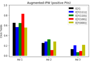
(a)

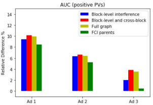
(b)

Figure 2: (a) Estimates of the counterfactual mean $\mathbb{E}[Y_{i}({\bf a})]$ for all possible allocations using AIPW. (b) Relative difference (in percentage) in AUCs with respect to the baseline model.

Recall that each allocation rule can be represented via a binary vector ${\bf a}=(a_{1},a_{2},a_{3}).$ As an example, the allocation $(1,1,1)$ corresponds to a scenario where all three ads are shown in the Top block. As mentioned in the preliminaries, ads are indexed according to the order in which they appear on the page. This indexing scheme restricts the state space of all possible allocation rules. For instance, an allocation like $(0,1,1)$ where the first positioned ad is placed at the Bottom and the rest are on Top is ill-defined and therefore excluded from the set of possible allocation rules.

We use AIPW to estimate the counterfactual mean $\mathbb{E}[Y_{i}({\bf a})]$ under all possible allocation rules for $\bf a.$ The results are shown in Figure 2(a). The layout that yields the highest click for each position on the pageview corresponds to the tallest bar on each plot. For instance, the first positioned ad benefits the most from being the sole ad in the Top block, i.e., $\mathbb{E}[Y_{1}(1,0,0)]>\mathbb{E}[Y_{1}({\bf a})],\forall{\bf a}\neq(1,0,0).$ However the corresponding optimal layout for the first positioned ad is not coherent with the optimal layout of other ads. For instance, the second positioned ad benefits the most from being on the Top block as well. On the other hand, the last positioned ad benefits slightly more when all ads are placed at the Bottom. In order to find a coherent optimal layout yielding the highest number of overall clicks, we need to compare the average click response over all positions on the pageview, i.e., the average overall effect $\frac{1}{m}\sum_{i=1}^{m}\ \mathbb{E}[Y_{i}({\bf a})],$ for all possible $\bf a$.

Table 1: Estimated values for the counterfactual mean $\mathbb{E}[Y_{i}({\bf a})]$ for all possible $\bf a,$ along with the $95\%$ confidence intervals. The observed $\mathbb{E}[Y_{i}]$ is reported on the last column.

	$\mathbb{E}[Y_{i}(1,1,1)]$	$\mathbb{E}[Y_{i}(1,1,0)]$	$\mathbb{E}[Y_{i}(1,0,0)]$	$\mathbb{E}[Y_{i}(0,0,0)]$	$\mathbb{E}[Y_{i}]$
First Ad	$0.57\ \pm\ 0.006$	$0.64\ \pm\ 0.004$	$0.83\ \pm\ 0.004$	$0.56\ \pm\ 0.005$	$0.65$
Second Ad	$0.28\ \pm\ 0.007$	$0.32\ \pm\ 0.005$	$0.11\ \pm\ 0.003$	$0.28\ \pm\ 0.005$	$0.25$
Third Ad	$0.20\ \pm\ 0.006$	$0.07\ \pm\ 0.002$	$0.09\ \pm\ 0.003$	$0.21\ \pm\ 0.005$	$0.13$

Estimated values for all the counterfactual means are reported in Table 1 along with the corresponding $95\%$ confidence intervals. We can use this table to compute various effects that were discussed in the previous section. For instance, the following contrast gives us the unit-level effect for $Y_{2}$ under allocation rule ${\bf a}=(1,0,0)$: $\text{UE}_{2}(1,0,{\bf a})=\mathbb{E}[Y_{2}(1,1,0)-Y_{2}(1,0,0)]=0.32-0.11=0.21\ (\pm 0.004).$ The spillover effect under allocation rules ${\bf a}=(1,0,0)$ and ${\bf a}^{\prime}=(1,1,1)$ is given by $\text{SE}_{2}(1,{\bf a^{\prime}},{\bf a})=\mathbb{E}[Y_{2}(1,1,1)-Y_{2}(1,1,0)]=0.28-0.32=-0.04\ (\pm 0.006).$ The overall effect of $\bf a$ versus ${\bf a}^{\prime},$ i.e., $\mathbb{E}[Y_{2}(1,1,1)-Y_{2}(1,0,0)]$ is equal to the sum of UE and SE which is $0.17\ (\pm 0.007).$

Learning the Causal Structure using FCI

In this part of the experiment, we use data to learn the parents of each outcome for all ads on the pageview; while allowing for both block-level and cross-block interference. We preprocess the data as described in Section 4.4, and use the implementation of the FCI algorithm in the Tetrad software. Independence tests are performed using kernel conditional independence tests (Zhang et al., 2012) with a significance level of $0.01.$ On each pageview, we collect $66$ different features. Neither plotting the learned graph nor enlisting all parental sets is relevant to the point we like to deliver here. Our primary objective is to show that for a particular positioned ad, features from other ads on the pageview (not necessarily from the same block even) are directly relevant to the clickability of the ad. In order for us to report the results in a more concise and clear way, we divide the ad-specific features into four distinct categories: (a) Calculated scores, such as PClick, PDefect, Relevance score, etc, (b) Decorative features, such as Twitter information, links, and ratings, (c) Geometric features, such as line counts, pixel heights, pixel heights from top of the block, and (d) match type information. We found out that the parent set of each $Y_{i}$ contains at least one variable in each category of features from a different ad; providing further evidence for the presence of interference among ads. In our extended set of experiments, we learned that Decorative features are more influential on pageviews with higher number of impressed ads.

Improvements in Click Prediction

Given the set of experiments described above, we are more confident to believe that interference does exist among ads. This was shown through both finding effects that are away from zero and learning causally relevant features that originate from other ads on the pageview. We now leverage this knowledge to better estimate the click yields. We considered fitting 5 different sets of models: (i) Baseline: $p(Y_{i}\mid L,X_{i}),$ (ii) Block-level interference: $p(Y_{i}\mid L,X_{i},\mathbb{I}(A_{j}=A_{i})\times X_{j}),$ (iii) Block-level and cross-block interference: $p(Y_{i}\mid L,X_{i},\mathbb{I}(A_{j}=A_{i})\times X_{j},\mathbb{I}(A_{k}\neq A_{i})\times X_{k}),$ (iv) Full graph with no block decomposition: $p(Y_{i}\mid L,X),$ and (v) fitting the model using parents in the output of FCI: $p(Y_{i}\mid\text{pa}(Y_{i})).$ We report relative improvements in area under the curve over the baseline in Figure 2(b). All methods that account for interference show improvement over the baseline over the baseline, demonstrating the utility of our formalization. It is also worth noting that the performance gains are greater for higher positioned ads compared to lower ones.

6 Conclusions

Despite the intuition that ads should not be scrutinized independently of one another, to the best of our knowledge, there has not been a formal analysis of interference in advertisement placement and sponsored search marketing. In this paper, we formalized the interference problem among ads using the language of causal inference and counterfactual reasoning. We proposed a framework to quantify the interference effects by posing a graphical causal model that accounts for potential underlying interference mechanisms. We described several causal effects that might be of interest in ad placement systems and discussed identification assumptions and estimation strategies for computing these effects.

References

- Bayir et al. [2019] Murat Ali Bayir, Mingsen Xu, Yaojia Zhu, and Yifan Shi. Genie: An open box counterfactual policy estimator for optimizing sponsored search marketplace. In Proceedings of the Twelfth ACM International Conference on Web Search and Data Mining, pages 465–473, 2019.
- Bhattacharya et al. [2019] Rohit Bhattacharya, Daniel Malinsky, and Ilya Shpitser. Causal inference under interference and network uncertainty. In Uncertainty in artificial intelligence: proceedings of the… conference. Conference on Uncertainty in Artificial Intelligence, volume 2019. NIH Public Access, 2019.
- Bhattacharya et al. [2020a] Rohit Bhattacharya, Razieh Nabi, and Ilya Shpitser. Semiparametric inference for causal effects in graphical models with hidden variables. arXiv preprint arXiv:2003.12659, 2020a.
- Bhattacharya et al. [2020b] Rohit Bhattacharya, Tushar Nagarajan, Daniel Malinsky, and Ilya Shpitser. Differentiable causal discovery under unmeasured confounding. arXiv preprint arXiv:2010.06978, 2020b.
- Bottou et al. [2013] Léon Bottou, Jonas Peters, Joaquin Quiñonero-Candela, Denis X Charles, D Max Chickering, Elon Portugaly, Dipankar Ray, Patrice Simard, and Ed Snelson. Counterfactual reasoning and learning systems: The example of computational advertising. The Journal of Machine Learning Research, 14(1):3207–3260, 2013.
- Cheng et al. [2012] Haibin Cheng, Roelof van Zwol, Javad Azimi, Eren Manavoglu, Ruofei Zhang, Yang Zhou, and Vidhya Navalpakkam. Multimedia features for click prediction of new ads in display advertising. In Proceedings of the 18th ACM SIGKDD international conference on Knowledge discovery and data mining, pages 777–785, 2012.
- Chickering [2002] David Maxwell Chickering. Optimal structure identification with greedy search. Journal of machine learning research, 3(Nov):507–554, 2002.
- Colombo and Maathuis [2014] Diego Colombo and Marloes H Maathuis. Order-independent constraint-based causal structure learning. The Journal of Machine Learning Research, 15(1):3741–3782, 2014.
- Effendi and Ali [2017] Muhammad Junaid Effendi and Syed Abbas Ali. Click through rate prediction for contextual advertisment using linear regression. arXiv preprint arXiv:1701.08744, 2017.
- Hill et al. [2015] Daniel N Hill, Robert Moakler, Alan E Hubbard, Vadim Tsemekhman, Foster Provost, and Kiril Tsemekhman. Measuring causal impact of online actions via natural experiments: Application to display advertising. In Proceedings of the 21th ACM SIGKDD International Conference on Knowledge Discovery and Data Mining, pages 1839–1847, 2015.
- Huang and Valtorta [2006] Yimin Huang and Marco Valtorta. Pearl’s calculus of intervention is complete. In Proceedings of the 22nd Conference on Uncertainty in Artificial Intelligence, pages 13–16, 2006.
- Hudgens and Halloran [2008] Michael G Hudgens and M Elizabeth Halloran. Toward causal inference with interference. Journal of the American Statistical Association, 103(482):832–842, 2008.
- Lauritzen [1996] Steffen L. Lauritzen. Graphical models. Oxford, U.K.: Clarendon, 1996.
- Nabi et al. [2018] Razieh Nabi, Phyllis Kanki, and Ilya Shpitser. Estimation of personalized effects associated with causal pathways. In Uncertainty in artificial intelligence: proceedings of the… conference. Conference on Uncertainty in Artificial Intelligence, volume 2018. NIH Public Access, 2018.
- Nabi-Abdolyousefi [2015] Razieh Nabi-Abdolyousefi. Conversion rate prediction in search engine marketing. PhD thesis, 2015.
- Ogburn et al. [2014] Elizabeth L Ogburn, Tyler J VanderWeele, et al. Causal diagrams for interference. Statistical science, 29(4):559–578, 2014.
- Pearl [2009] Judea Pearl. Causality. Cambridge University Press, 2009.
- Richardson and Robins [2013] Thomas S. Richardson and James M. Robins. Single world intervention graphs (SWIGs): A unification of the counterfactual and graphical approaches to causality. Center for the Statistics and the Social Sciences, University of Washington Series. Working Paper, 128(30), 2013.
- Richardson and Spirtes [2002] Thomas S. Richardson and Peter L. Spirtes. Ancestral graph Markov models. The Annals of Statistics, 30(4):962–1030, 2002.
- Richardson et al. [2017] Thomas S. Richardson, Robin J. Evans, James M. Robins, and Ilya Shpitser. Nested Markov properties for acyclic directed mixed graphs. arXiv preprint arXiv:1701.06686, 2017.
- Robins [1986] James M. Robins. A new approach to causal inference in mortality studies with a sustained exposure period – application to control of the healthy worker survivor effect. Mathematical Modelling, 7(9-12):1393–1512, 1986.
- Rubin [1980] Donald B Rubin. Randomization analysis of experimental data: The fisher randomization test comment. Journal of the American Statistical Association, 75(371):591–593, 1980.
- Shalizi and Thomas [2011] Cosma Rohilla Shalizi and Andrew C Thomas. Homophily and contagion are generically confounded in observational social network studies. Sociological methods & research, 40(2):211–239, 2011.
- Sherman and Shpitser [2018] Eli Sherman and Ilya Shpitser. Identification and estimation of causal effects from dependent data. In Advances in Neural Information Processing Systems, pages 9424–9435, 2018.
- Shpitser [2013] Ilya Shpitser. Counterfactual graphical models for longitudinal mediation analysis with unobserved confounding. Cognitive science, 37(6):1011–1035, 2013.
- Shpitser and Pearl [2006] Ilya Shpitser and Judea Pearl. Identification of joint interventional distributions in recursive semi-Markovian causal models. In Proceedings of the 21st National Conference on Artificial Intelligence, 2006.
- Shpitser and Pearl [2012] Ilya Shpitser and Judea Pearl. Identification of conditional interventional distributions. arXiv preprint arXiv:1206.6876, 2012.
- Sobel [2006] Michael E Sobel. What do randomized studies of housing mobility demonstrate? causal inference in the face of interference. Journal of the American Statistical Association, 101(476):1398–1407, 2006.
- Spirtes et al. [2000] Peter Spirtes, Clark N Glymour, Richard Scheines, and David Heckerman. Causation, prediction, and search. MIT press, 2000.
- Tchetgen and VanderWeele [2012] Eric J Tchetgen Tchetgen and Tyler J VanderWeele. On causal inference in the presence of interference. Statistical methods in medical research, 21(1):55–75, 2012.
- Tian and Pearl [2002] Jin Tian and Judea Pearl. A general identification condition for causal effects. In Proceedings of the 18th National Conference on Artificial Intelligence, pages 567–573. American Association for Artificial Intelligence, 2002.
- Verma and Pearl [1990] Thomas Verma and Judea Pearl. Equivalence and synthesis of causal models. In Proceedings of the 6th Conference on Uncertainty in Artificial Intelligence, 1990.
- Xiong et al. [2012] Chenyan Xiong, Taifeng Wang, Wenkui Ding, Yidong Shen, and Tie-Yan Liu. Relational click prediction for sponsored search. In Proceedings of the fifth ACM international conference on Web search and data mining, pages 493–502, 2012.
- Yin et al. [2014] Dawei Yin, Bin Cao, Jian-Tao Sun, and Brian D Davison. Estimating ad group performance in sponsored search. In Proceedings of the 7th ACM international conference on Web search and data mining, pages 143–152, 2014.
- Zeng et al. [2019] Shuxi Zeng, Emre Kiciman, Denis Charles, Joel Pfeiffer, and Murat Ali Bayir. Causal transfer random forest: Leveraging observational and randomization studies. 2019.
- Zhang [2008] Jiji Zhang. On the completeness of orientation rules for causal discovery in the presence of latent confounders and selection bias. Artificial Intelligence, 172(16-17):1873–1896, 2008.
- Zhang et al. [2012] Kun Zhang, Jonas Peters, Dominik Janzing, and Bernhard Schölkopf. Kernel-based conditional independence test and application in causal discovery. arXiv preprint arXiv:1202.3775, 2012.
- Zhang et al. [2014] Yuyu Zhang, Hanjun Dai, Chang Xu, Jun Feng, Taifeng Wang, Jiang Bian, Bin Wang, and Tie-Yan Liu. Sequential click prediction for sponsored search with recurrent neural networks. arXiv preprint arXiv:1404.5772, 2014.
- Zheng et al. [2018] Xun Zheng, Bryon Aragam, Pradeep K Ravikumar, and Eric P Xing. Dags with no tears: Continuous optimization for structure learning. In Advances in Neural Information Processing Systems, pages 9472–9483, 2018.