Boosting One-Point Derivative-Free Online Optimization via Residual Feedback
Abstract
Zeroth-order optimization (ZO) typically relies on two-point feedback to estimate the unknown gradient of the objective function. Nevertheless, two-point feedback can not be used for online optimization of time-varying objective functions, where only a single query of the function value is possible at each time step. In this work, we propose a new one-point feedback method for online optimization that estimates the objective function gradient using the residual between two feedback points at consecutive time instants. Moreover, we develop regret bounds for ZO with residual feedback for both convex and nonconvex online optimization problems. Specifically, for both deterministic and stochastic problems and for both Lipschitz and smooth objective functions, we show that using residual feedback can produce gradient estimates with much smaller variance compared to conventional one-point feedback methods. As a result, our regret bounds are much tighter compared to existing regret bounds for ZO with conventional one-point feedback, which suggests that ZO with residual feedback can better track the optimizer of online optimization problems. Additionally, our regret bounds rely on weaker assumptions than those used in conventional one-point feedback methods. Numerical experiments show that ZO with residual feedback significantly outperforms existing one-point feedback methods also in practice.
1 Introduction
Zeroth-order optimization (ZO) algorithms have been widely used to solve online optimization problems where first or second order information (i.e., gradient or Hessian information) is unavailable at each time instant. Such problems arise, e.g., in online learning and involve adversarial training Chen et al. (2017) and reinforcement learning Fazel et al. (2018); Malik et al. (2018) among others. The goal is to minimize a sequence of time-varying objective functions , where the value is revealed to the agent after an action is selected and is used to adapt the agent’s future strategy. Since the objective functions are not known a priori, the quality of an online decision can be measured using notions of regret, that generally compare the total cost incurred by an online decision to the cost of the fixed or varying optimal decision that a clairvoyant agent could select.
Perhaps the most popular zeroth-order gradient estimator is the two-point estimator that has been extensively studied in Agarwal et al. (2010); Ghadimi & Lan (2013); Duchi et al. (2015); Bach & Perchet (2016); Nesterov & Spokoiny (2017); Gao et al. (2018); Roy et al. (2019). This estimator queries the function value twice at each time step, and uses the difference in the two function values to estimate the desired gradient, i.e.,
| (Two-point | (1) |
where is a parameter and . Although this two-point estimator produces gradient estimates with low variance that improve the convergence speed of ZO, it can not be used for non-stationary online optimization problems that arise frequently in online learning. The reason is that in these non-stationary online optimization problems, the objective function being queried is time-varying, and hence only a single function value can be sampled at a given time instant. In this case, one-point estimators can be used instead that query the objective function only once at each time instant, i.e.,
| (One-point | (2) |
One-point feedback was first proposed and analyzed in Flaxman et al. (2005) for convex online optimization problems. Saha & Tewari (2011); Dekel et al. (2015) showed that the regret of convex online optimization methods using one-point gradient estimation can be improved if the objective functions are assumed to be smooth and self-concordant regularization is used. More recently, Gasnikov et al. (2017) developed regret bounds for ZO with one-point feedback also for stochastic convex problems. On the other hand, Hazan et al. (2016) characterized the convergence of one-point zeroth-order methods for static stochastic non-convex optimization problems. However, as shown in these studies, one-point feedback produces gradient estimates with large variance which results in increased regret. In addition, the regret analysis for ZO with one-point feedback usually requires the strong assumption that the function value is uniformly upper bounded over time, so this method can not be used for practical non-stationary optimization problems.
Contributions: In this paper, we propose a novel one-point gradient estimator for zeroth-order online optimization and develop new regret bounds to study its performance. Our proposed estimator uses the residual between two consecutive feedback points to estimate the gradient and, therefore, we refer to it as residual feedback. We show that, for both deterministic and stochastic problems, using residual feedback produces gradient estimates with lower variance compared to those produced using the conventional one-point feedback proposed in Flaxman et al. (2005); Gasnikov et al. (2017). As a result, we obtain tighter regret bounds both for convex and non-convex problems, especially when the value of the objective function is large. Moreover, our regret analysis relies on weaker assumptions compared to those for ZO with conventional one-point feedback. Finally, we present numerical experiments that demonstrate that ZO with residual feedback significantly outperforms the conventional one-point method in its ability to track the time-varying optimizers of online learning problems. To the best of our knowledge, this is the first time a one-point zeroth-order method is theoretically studied for non-convex online optimization problems. It is also the first time that a one-point gradient estimator demonstrates comparable empirical performance to that of the two-point method. We note that two-point estimators can only be used to solve non-stationary online learning problems in simulation, where the system can be reset to the same fixed state during two different queries of the objective function values at a given time instant.
Related work: Online optimization problems are only one instance of optimization problems that ZO methods have been used to solve. For example, Balasubramanian & Ghadimi (2018) apply ZO to solve a set-constrained optimization problem where the projection onto the constraint set is non-trivial. Gorbunov et al. (2018); Ji et al. (2019) apply a variance-reduced technique and acceleration schemes to achieve better convergence speed in ZO. Wang et al. (2018) improve the dependence of the iteration complexity on the dimension of the problem under an additional sparsity assumption on the gradient of the objective function. Finally, Hajinezhad & Zavlanos (2018); Tang & Li (2019) apply zeroth-order oracles to distributed optimization problems when only bandit feedbacks are available at each local agents. Our proposed residual feedback oracle can be used to solve such optimization problems as well. Also related is work by Zhang et al. (2015) that considers non-convex online bandit optimization problems with a single query at each time step. However, this method employs the exploration and exploitation bandit learning framework and the proposed analysis is restricted to a special class of non-convex objective functions. Finally, Agarwal et al. (2011); Hazan & Li (2016); Bubeck et al. (2017) study online bandit algorithms using ellipsoid methods. In particular, these methods induce heavy computation per step and achieve regret bounds that have bad dependence on the problem dimension. As a comparison, our one-point method is computation light and achieves regret bounds that have better dependence on the problem dimension.
2 Preliminaries and Residual Feedback
In this section we provide basic definitions and results on ZO that will be needed in the subsequent analysis. We also define the residual feedback gradient estimator that we propose to solve online optimization problems with unknown gradient information. First, we define the class of Lipschitz and smooth objective functions we are concerned with.
Definition 2.1 (Lipschitz functions).
The class of Lipschtiz-continuous functions satisfies: for any , , where is the Lipschitz parameter. The class of smooth functions satisfies: for any , where is the smoothness parameter.
The key idea in ZO is to estimate the unknown first-order gradient of the objective function using zeroth-order oracles that perturb the objective function around the current point along all directions uniformly. The ability of these oracles to correctly estimate the gradient is typically analyzed using the Gaussian-smoothed version of the function defined as , where the coordinates of the vector are i.i.d standard Gaussian random variables; see Nesterov & Spokoiny (2017). The following result bounds the approximation error of the function and can be found in Nesterov & Spokoiny (2017).
Lemma 2.2.
Consider a function and its smoothed version . It holds that
The smoothed function also satisfies the following amenable property; see Nesterov & Spokoiny (2017).
Lemma 2.3.
If is -Lipschitz, then with Lipschitz constant .
In this paper we consider the following online bandit optimization problem
| (P) |
where is a convex set and is a random sequence of objective functions. We assume that at time , a new objective function is randomly generated independent of an agent’s decisions, the objective functions are unknown a priori and their derivatives are unavailable but can be estimated using a zeroth-order oracle that queries the objective function value at different perturbed points , as discussed above. The goal is to determine an online decision with cost that is as close as possible to the cost of a fixed or varying optimal decision that a clairvoyant agent could select, which is measured using notions of regret.
Such online optimization problems often arise in non-stationary learning, where the system is time-varying or a single query of the function changes the system state (i.e., changes to ). In these problems, two-point feedback can not be used to estimate the unknown gradient as it requires to evaluate at two different points at the same time . Instead, a more practical approach is to use the one-point feedback scheme (2) in Gasnikov et al. (2017). However, the gradient estimates produced by the one-point feedback method in (2) have large variance that leads to large regret and, therefore, poor ability to track the optimizer of the online problem. To address this limitation, in this paper we propose a novel one-point gradient estimator, which we call a one-point residual feedback estimator, that has reduced variance and is defined as
| (3) |
where are independent random vectors. To elaborate, the proposed residual feedback estimator in (3) queries at a single perturbed point , and then subtracts the value obtained from the previous iteration. Next, we discuss some basic properties of this new estimator. We first show that this estimator provides an unbiased gradient estimate of the smoothed function .
Lemma 2.4.
The residual feedback estimator satisfies for all and .
Proof.
The proof follows from the fact that has zero mean and is independent from and . ∎
Remark 2.5.
We note that existing two-point estimators can not be easily modified to be used for non-stationary optimization. The difficulty is in ensuring that the returned gradient estimates are unbiased as in the case of residual feedback in Lemma 2.4. To see this, consider the simple modification of the online two-point gradient estimator (7) proposed in Bach & Perchet (2016)
Then, it is easy to see that this modified two-point gradient estimator is biased since . Specifically, let , where . Although , we have that since is correlated with . Therefore, for this modified estimator we have that . Note that the original two-point estimator proposed in Bach & Perchet (2016) is unbiased, because the function is queried at two points, and , and the noise in this case is simply the evaluation noise that is zero mean for any .
In this paper, we consider the following ZO projected gradient update with residual feedback to solve the online problem (P):
| (4) |
where is the learning rate and is the projection operator onto the set . The update (4) can be implemented assuming that the objective function can be queried at points outside the feasible set , similar to the methods considered in Duchi et al. (2015); Bach & Perchet (2016); Gasnikov et al. (2017). Note that it is possible to modify the update (4) so that the iterates are guaranteed to be within the feasible set . This modification and related analysis can be found in Section H in the supplementary material. The requirement that the objective function is evaluated at feasible points in derivative-free optimization algorithms has also been considered in Bubeck et al. (2017); Bilenne et al. (2020). Specifically, Bubeck et al. (2017) develop the so called ellipsoid method, which requires computation of an ellipsoid containing the optimizer at each time step. On the other hand, almost concurrently with this work, Bilenne et al. (2020) proposed a similar oracle as in (3) for a static convex optimization problem with specific objective and constraint functions. The following result bounds the second moment of the gradient estimate generated by using residual feedback.
Lemma 2.6 (Second moment).
Assume that with Lipschitz constant for all time . Then, under the ZO update rule in (4), the second moment of the residual feedback satisfies:
| (5) |
where .
The proof of above lemma can be found in Appendix B. The above lemma shows that the second moment of the gradient estimates obtained using residual feedback forms a contraction with perturbation term , provided that we choose and such that the contracting rate satisfies . As we show later in the analysis, this contraction property leads to gradient estimates with low variance that allow to reduce the regret of the online ZO algorithm (4).
3 ZO with Residual Feedback for Convex Online Optimization
In this section, we consider the online bandit problem (P) where the sequence of functions are all convex. In particular, we are interested in analyzing the static regret of algorithm (4) defined as
| (6) |
First, we make the following assumption on the non-stationarity of the online learning problem.
Assumption 3.1 (Bounded variation).
There exists such that for all ,
| (7) |
where the expectation is taken over , the random vector and the random functions ,.
Assumption 3.1 states that the squared variation of the objective function between two consecutive time instants is uniformly bounded over time. We note that this assumption is weaker than the assumption that the objective function is uniformly bounded, i.e., , which is used in the analysis of ZO with conventional one-point feedback in Flaxman et al. (2005); Gasnikov et al. (2017). In particular, under Assumption 3.1, the perturbation term in Lemma 2.6 can be bounded as . Then, by telescoping the contraction inequality, we obtain the following bound for the second moment of the residual-feedback gradient estimate
| (8) |
The detailed proof can be found in Appendix J. In practice, needs to be sufficiently small so that the smoothed function is close to the original function according to Lemma 2.2. In this case, the above bound on the second moment of the residual-feedback gradient estimates is dominated by , which is much smaller than the bound on the second moment of the conventional one-point gradient estimates , where is the uniform bound on over time. For example, consider the time-varying objective functions, and , where is Gaussian noise with zero mean at time . Then, it can be verified that Assumption 3.1 holds with a finite whereas the second moment of is unbounded over time. As a result, the variance of the residual feedback gradient estimates can be significantly smaller than that of the conventional one-point feedback gradient estimates.
The following result characterizes the regret of ZO with residual feedback when the objective function is convex and Lipschitz.
Theorem 3.2 (Regret for Convex Lipschitz ).
Let Assumption 3.1 hold. Assume that is convex with Lipschitz constant for all and . Run ZO with residual feedback for iterations with and . Then, we have that
| (9) |
Asymptotically, we have .
The proof can be found in Appendix C. To the best of our knowledge, the best known regret for ZO with conventional one-point feedback is of the order Gasnikov et al. (2017). Therefore, our regret bound is tighter if the function variation satisfies . Essentially, using the proposed residual feedback gradient estimator, the regret of ZO no longer depends on the uniform bound of the function value, which can be very large in practice. Instead, our regret only relies on how fast the function varies over time. Note that knowledge of the neighborhood in Theorem 3.2 allows to select the stepsize and the parameter so that a better regret rate can be achieved that depends on . However, knowledge of is not required and ZO with residual feedback converges from any initial point . When the parameter is unknown, we can choose and and obtain the regret bound . The proof can be found in Appendix C.
Remark 3.3.
We note that the complexity bound in Theorem 3.2 generally depends on the values of the Lipschitz parameters , and the constant . Specifically, choose and with as a tuning parameter, and we obtain that when . If , we can choose to achieve the bound . On the other hand, if , we can choose to achieve the bound . We note that the dependence of the bounds in Theorems 3.4, 4.2 and 4.3 on can also be optimized in a similar way by properly choosing .
Next, we present the regret of ZO with residual feedback when the objective function is convex and smooth.
Theorem 3.4 (Regret for Convex Smooth ).
Let Assumption 3.1 hold. Assume that is convex with Lipschitz constant and smoothness constant for all , and assume that . Run ZO with residual feedback for iterations with and . Then, we have that
| (10) |
Asymptotically, we have that .
The proof can be found in Appendix D. To the best of our knowledge, the best known regret for ZO with conventional one-point feedback for convex and smooth problems is of the order Gasnikov et al. (2017). Therefore, our regret bound is tighter if the function variation satisfies . Our numerical experiments in Section 6 show that ZO with residual feedback always outperforms ZO with conventional one-point feedback in practice.
4 ZO with Residual Feedback for Non-Convex Online Optimization
In this section, we analyze the regret of ZO with residual feedback for the unconstrained online bandit problem (P) where the objective functions are non-convex. To the best of our knowledge, this is the first time that a one-point zeroth-order method is studied for non-convex online optimization. Throughout this section, we make the following assumption on the objective functions.
Assumption 4.1.
There exist such that the following conditions hold for all .
-
1.
, where the expectation is taken with respect to and the random smoothed objective functions , .
-
2.
, where the expectation is taken with respect to , the random vector and the random objective functions , .
The above two conditions in Assumption 4.1 measure the accumulated first-order and second-order function variations. A similar assumption is made in Roy et al. (2019).
First, we consider the case where are nonconvex and Lipschitz continuous functions. Since the objective function is not necessarily differentiable, i.e., is not well defined, we define the regret as the accumulated gradient of the smoothed function, i.e., In addition, similar to Nesterov & Spokoiny (2017), we require that the smoothed function is close to the original function such that for all . To satisfy this condition, we need to choose according to Lemma 2.2. Then, we can show the following regret bound for ZO with residual feedback.
Theorem 4.2 (Nonconvex Lipschitz ).
Let Assumptions 4.1 hold. Assume that with Lipschitz constant and that is bounded below by for all . Run ZO with residual feedback for iterations with and . Then, we have that
| (11) |
Asymptotically, we have .
The proof can be found in Appendix E. Theorem 4.2 implies that the regret bound satisfies whenever and . In particular, if the bounded variation Assumption 4.1 holds, then we have , and it suffices to let .
Next, we assume that the objective functions in (P) are non-convex and smooth and study the regret . Specifically, we provide the following regret bound for ZO with residual-feedback.
Theorem 4.3 (Nonconvex smooth ).
Let Assumptions 4.1 hold. Assume that with Lipschitz constant and smoothness constant and that is bounded below by for all . Run ZO with residual feedback for iterations with and . Then,
| (12) |
Asymptotically, we have that .
5 ZO with Residual Feedback for Stochastic Online Optimization
Our proposed residual feedback gradient estimator can be also extended to solve stochastic online bandit problems. Since the regret analysis is similar to that for deterministic online problems presented before, we only introduce the key technical lemmas and comment on the differences in the proof. Specifically, we consider the following stochastic online bandit problems
| (R) |
where denotes a certain noise that is independent of . Different from the deterministic online problems discussed before, the agent here can only query noisy evaluations of the objective function. This covers scenarios where the agent does not have access to the underlying data distribution. To solve the above stochastic online problem, we propose the following stochastic residual feedback
| (13) |
where and are independent random samples that are sampled at consecutive iterations and , respectively. Since the noisy function value is an unbiased estimate of the objective function , it is straightforward to show that (13) is an unbiased gradient estimate of the function . To analyze the regret of ZO with stochastic residual feedback, we first consider the convex case and make the following assumption on the variation of the stochastic objective functions.
Assumption 5.1.
(Bounded stochastic variation) There exists such that for all ,
where the expectation is taken with respect to , the random vector and the random objective functions , .
The above assumption generalizes Assumption 3.1 to stochastic problems. The bound controls both the variation of function over time and the variation due to stochastic sampling.
The following lemma characterizes the second moment of the stochastic residual feedback gradient estimates. Its proof can be found in Appendix G.
Lemma 5.2.
Assume with Lipschitz constant for all . Then, under the ZO update rule, we have that
where .
Observe that the above second moment bound is very similar to that in Lemma 2.6, and the only difference is the perturbation term. Since the perturbation term can be further bounded by leveraging Assumption 5.1, the resulting second moment bound can become almost the same as that in eq. 8 for deterministic problems (simply replace in eq. 8 by ). Therefore, the regret analysis of ZO with stochastic residual feedback is the same as that of ZO with residual feedback for deterministic online problems. Consequently, ZO with stochastic residual feedback achieves almost the same regret bounds as those in Theorems 3.2 and 3.4, and one simply needs to replace by .
In the case of non-convex stochastic online problems, we adopt the following assumption that generalizes Assumption 4.1.
Assumption 5.3.
There exists such that the following two conditions hold for all .
-
1.
, where the expectation is taken with respect to and the random smoothed objective functions , .
-
2.
, where the expectation is taken with respect to , the random vector and the random objective functions , .
6 Numerical Experiments
In this section, we compare the performance of ZO with one-point, two-point and residual feedback in solving two non-stationary reinforcement learning problems, i.e., LQR control and resource allocation, in which either the reward or transition functions are varying over episodes.
6.1 Nonstatinoary LQR Control
We consider an LQR problem with noisy system dynamics. The static version of this problem is considered in Fazel et al. (2018); Malik et al. (2018). Specifically, consider a system whose state at step is subject to a transition function , where is the action at step , and and are dynamical matrices in episode . These matrices are unknown and changing over episodes. The vector is the noise on the state transition. Specifically, the entries of the dynamical matrices and at episode are randomly generated from a Gaussian distribution . Then, we generate the time-varying dynamical matrices as and , where and are random matrices whose entries are uniformly sampled from [0,1]. Moreover, consider a state feedback policy , where is the policy parameter that is fixed during episode . We assume that there exists an optimal policy so that the discounted accumulated cost function at episode is minimized, where is the discount factor and is the horizon. The goal is to track the time-varying optimal policy parameter so that is small in every episode.
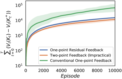
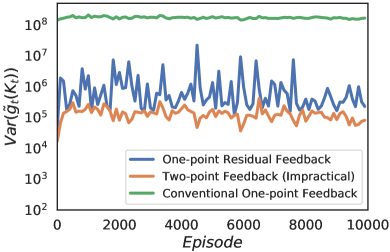
We apply the conventional one-point method in Gasnikov et al. (2017) and the proposed residual-feedback method (13) to solve the above non-stationary LQR problem. The performance of the two-point method in Bach & Perchet (2016) is also presented to serve as a benchmark, although it is not possible to implement in practice for non-stationary problems. This is because the two-point method in Bach & Perchet (2016) requires to evaluate value function for two different policy functions at two consecutive episodes. However, evaluating the value function for a given policy during episode requires to collect samples by executing this policy. Then, during the subsequent episode , since the problem is non-stationary, the dynamic matrices change to and so does the value function . Therefore, it is not possible to evaluate the same value function at two different episodes and, as a result, the two-point method in Bach & Perchet (2016) is not applicable here. Each algorithm is run for trials, and the stepsizes are optimized for each algorithm separately. The accumulated regrets of the three algorithms are presented in Figure 1(a). We observe that ZO with residual feedback achieves a much lower regret than the conventional one-point method and has a comparable performance to that of the two-point method. Moreover, we present in Figure 1(b) the estimated variance of the gradient estimates returned by these three oracles at the policy iterates over episodes. It can be seen that the variance of the gradient estimates returned by our proposed residual-feedback is close to that of the gradient estimates returned by the two-point feedback and is much smaller than that of the gradient estimates returned by the conventional one-point feedback. This observation validates our theoretical characterization of the second moment of the residual feedback gradient estimates.
6.2 Nonstationary Resource Allocation
We consider a multi-stage resource allocation problem with time-varying sensitivity to the lack of resource supply. Specifically, agents are located on a grid. During episode , at step , agent stores amount of resources and has a demand for resources in the amount of . Also, agent decides to send a fraction of resources to its neighbors on the grid. The local amount of resources and demands of agent evolve as and , where is the noise in the demand. At each step , agent receives a local cost , such that when and when , where represents the varying sensitivity of the agents to the lack of supply during episode . Let agent makes its decisions according to a parameterized policy function , where is the parameter of the policy function at episode , denotes agent ’s local observation. Specifically, we let . Our goal is to track the time-varying optimal policy so that the accumulated cost over the grid during each episode is maintained at a low level, where is the policy parameter, is the problem horizon at each episode, and is the discount factor.
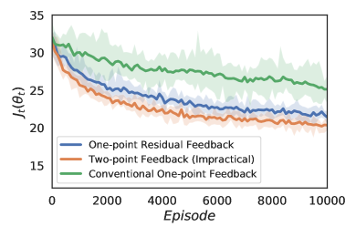
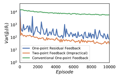
In Figure 2(a), we present the cost achieved during each episode after trials of ZO with residual-feedback, one-point, and two-point feedback which, as before, is impossible to use in practice for this non-stationary problem either. It can be seen that ZO with our proposed residual-feedback achieves a cost that is as low as the cost achieved by the two-point feedback in this non-stationary environment. In particular, ZO with both residual and two-point feedback performs much better than ZO with conventional one-point feedback. Figure 2(b) also compares the estimated variance of the gradient estimates returned by these feedback schemes. It can be seen that the variance of the gradient estimates returned by the residual feedback oracle is comparable to that of the gradient estimates returned by the two-point oracle and is much smaller than that of the gradient estimates returned by the conventional one-point oracle.
7 Conclusion
In this paper, we proposed a novel one-point residual feedback oracle for zeroth-order online optimization, which estimates the gradient of the time-varying objective function using a single query of the function value at each time instant. For both deterministic and stochastic problems, we showed that ZO with the proposed residual feedback estimator achieves much lower regret than that of ZO with conventional one-point feedback for convex online optimization problems. In addition, we provided regret bounds for ZO with residual feedback for non-convex online optimization problems. To the best of our knowledge, this is the first time that a one-point zeroth-order method is theoretically studied for non-convex online problems. Numerical experiments on two non-stationary reinforcement learning problems were conducted and the proposed residual-feedback estimator was shown to significantly outperform the conventional one-point method.
References
- Agarwal et al. (2010) Alekh Agarwal, Ofer Dekel, and Lin Xiao. Optimal algorithms for online convex optimization with multi-point bandit feedback. In COLT, pp. 28–40. Citeseer, 2010.
- Agarwal et al. (2011) Alekh Agarwal, Dean P Foster, Daniel J Hsu, Sham M Kakade, and Alexander Rakhlin. Stochastic convex optimization with bandit feedback. In Advances in Neural Information Processing Systems, pp. 1035–1043, 2011.
- Bach & Perchet (2016) Francis Bach and Vianney Perchet. Highly-smooth zero-th order online optimization. In Conference on Learning Theory, pp. 257–283, 2016.
- Balasubramanian & Ghadimi (2018) Krishnakumar Balasubramanian and Saeed Ghadimi. Zeroth-order (non)-convex stochastic optimization via conditional gradient and gradient updates. In Advances in Neural Information Processing Systems, pp. 3455–3464, 2018.
- Bilenne et al. (2020) Olivier Bilenne, Panayotis Mertikopoulos, and Elena-Veronica Belmega. Fast optimization with zeroth-order feedback in distributed, multi-user mimo systems. IEEE Transactions on Signal Processing, 2020.
- Bubeck et al. (2012) Sébastien Bubeck, Nicolo Cesa-Bianchi, et al. Regret analysis of stochastic and nonstochastic multi-armed bandit problems. Foundations and Trends® in Machine Learning, 5(1):1–122, 2012.
- Bubeck et al. (2017) Sébastien Bubeck, Yin Tat Lee, and Ronen Eldan. Kernel-based methods for bandit convex optimization. In Proceedings of the 49th Annual ACM SIGACT Symposium on Theory of Computing, pp. 72–85, 2017.
- Chen et al. (2017) Pin-Yu Chen, Huan Zhang, Yash Sharma, Jinfeng Yi, and Cho-Jui Hsieh. Zoo: Zeroth order optimization based black-box attacks to deep neural networks without training substitute models. In Proceedings of the 10th ACM Workshop on Artificial Intelligence and Security, pp. 15–26, 2017.
- Dekel et al. (2015) Ofer Dekel, Ronen Eldan, and Tomer Koren. Bandit smooth convex optimization: Improving the bias-variance tradeoff. In Advances in Neural Information Processing Systems, pp. 2926–2934, 2015.
- Duchi et al. (2015) John C Duchi, Michael I Jordan, Martin J Wainwright, and Andre Wibisono. Optimal rates for zero-order convex optimization: The power of two function evaluations. IEEE Transactions on Information Theory, 61(5):2788–2806, 2015.
- Fazel et al. (2018) Maryam Fazel, Rong Ge, Sham Kakade, and Mehran Mesbahi. Global convergence of policy gradient methods for the linear quadratic regulator. In Proceedings of the 35th International Conference on Machine Learning, volume 80, 2018.
- Flaxman et al. (2005) Abraham D Flaxman, Adam Tauman Kalai, and H Brendan McMahan. Online convex optimization in the bandit setting: gradient descent without a gradient. In Proceedings of the sixteenth annual ACM-SIAM symposium on Discrete algorithms, pp. 385–394. Society for Industrial and Applied Mathematics, 2005.
- Gao et al. (2018) Xiand Gao, Xiaobo Li, and Shuzhong Zhang. Online learning with non-convex losses and non-stationary regret. In International Conference on Artificial Intelligence and Statistics, pp. 235–243, 2018.
- Gasnikov et al. (2017) Alexander V Gasnikov, Ekaterina A Krymova, Anastasia A Lagunovskaya, Ilnura N Usmanova, and Fedor A Fedorenko. Stochastic online optimization. single-point and multi-point non-linear multi-armed bandits. convex and strongly-convex case. Automation and remote control, 78(2):224–234, 2017.
- Ghadimi & Lan (2013) Saeed Ghadimi and Guanghui Lan. Stochastic first-and zeroth-order methods for nonconvex stochastic programming. SIAM Journal on Optimization, 23(4):2341–2368, 2013.
- Gorbunov et al. (2018) Eduard Gorbunov, Pavel Dvurechensky, and Alexander Gasnikov. An accelerated method for derivative-free smooth stochastic convex optimization. arXiv preprint arXiv:1802.09022, 2018.
- Hajinezhad & Zavlanos (2018) Davood Hajinezhad and Michael M Zavlanos. Gradient-free multi-agent nonconvex nonsmooth optimization. In 2018 IEEE Conference on Decision and Control (CDC), pp. 4939–4944. IEEE, 2018.
- Hazan & Li (2016) Elad Hazan and Yuanzhi Li. An optimal algorithm for bandit convex optimization. arXiv preprint arXiv:1603.04350, 2016.
- Hazan et al. (2016) Elad Hazan, Kfir Yehuda Levy, and Shai Shalev-Shwartz. On graduated optimization for stochastic non-convex problems. In International conference on machine learning, pp. 1833–1841, 2016.
- Ji et al. (2019) Kaiyi Ji, Zhe Wang, Yi Zhou, and Yingbin Liang. Improved zeroth-order variance reduced algorithms and analysis for nonconvex optimization. arXiv preprint arXiv:1910.12166, 2019.
- Malik et al. (2018) Dhruv Malik, Ashwin Pananjady, Kush Bhatia, Koulik Khamaru, Peter L Bartlett, and Martin J Wainwright. Derivative-free methods for policy optimization: Guarantees for linear quadratic systems. arXiv preprint arXiv:1812.08305, 2018.
- Nesterov (2013) Yurii Nesterov. Introductory lectures on convex optimization: A basic course, volume 87. Springer Science & Business Media, 2013.
- Nesterov & Spokoiny (2017) Yurii Nesterov and Vladimir Spokoiny. Random gradient-free minimization of convex functions. Foundations of Computational Mathematics, 17(2):527–566, 2017.
- Roy et al. (2019) Abhishek Roy, Krishnakumar Balasubramanian, Saeed Ghadimi, and Prasant Mohapatra. Multi-point bandit algorithms for nonstationary online nonconvex optimization. arXiv preprint arXiv:1907.13616, 2019.
- Saha & Tewari (2011) Ankan Saha and Ambuj Tewari. Improved regret guarantees for online smooth convex optimization with bandit feedback. In Proceedings of the Fourteenth International Conference on Artificial Intelligence and Statistics, pp. 636–642, 2011.
- Tang & Li (2019) Yujie Tang and Na Li. Distributed zero-order algorithms for nonconvex multi-agent optimization. In 2019 57th Annual Allerton Conference on Communication, Control, and Computing (Allerton), pp. 781–786. IEEE, 2019.
- Wang et al. (2018) Yining Wang, Simon Du, Sivaraman Balakrishnan, and Aarti Singh. Stochastic zeroth-order optimization in high dimensions. In International Conference on Artificial Intelligence and Statistics, pp. 1356–1365, 2018.
- Zhang et al. (2015) Lijun Zhang, Tianbao Yang, Rong Jin, and Zhi-Hua Zhou. Online bandit learning for a special class of non-convex losses. In AAAI, pp. 3158–3164, 2015.
Appendix
Appendix A Implementation Details of the Numerical Experiments
All experiments are conducted using Matlab R2019a on Ubuntu 18.04 with the AMD Ryzen 2700X 8-core processor and 16GB 2133MHz memory.
For the non-stationary LQR experiments, we select , and . The dynamical matrices and at episode are randomly generated from a Gaussian distribution . Then, we generate the time-varying dynamical matrices according to and , where and are random matrices whose entries are uniformly sampled from [0,1]. To evaluate the cost function given the policy parameter at episode , we roll out a trajectory of length using the policy parameter and sum up the collected rewards.
For the non-stationary resource allocation experiments, the policy function is parameterized as: , where and and the episode index is omitted for notational simplicity. Specifically, the feature function is selected as , where is the parameter of the -th feature function. Effectively, the agents need to make decisions on actions, and each action is decided by parameters. Therefore, the problem dimension is . The discount factor is selected as and the length of the horizon is . The time-varying sensitivity parameter is generated as follows: let and , where is a random number uniformly sampled from .
Appendix B Proof of Lemma 2.6
By definition of the residual feedback, we have
| (14) |
Since is independent of , and the generation of functions and , we have that . Moreover, adding and subtracting in the term of the above inequality, we obtain that
| (15) |
Since is Lipschitz with constant , we further obtain that
| (16) |
Note that is a Gaussian vector independent from , we then obtain that Furthermore, using Lemma 1 in Nesterov & Spokoiny (2017), we know that . Substituting these bounds into inequality (B), we obtain that
Since , we get that due to the nonexpansiveness of the projection operator onto a convex set. Therefore, we have that
The proof is complete.
Appendix C Proof of Theorem 3.2
Note that is convex for all , we then conclude that
| (17) |
Adding and subtracting after in above inequality, and taking expectation over on both sides, we obtain that
| (18) |
Since , for any we have that
| (19) |
Rearranging the above inequality yields that
| (20) |
Taking expectation on both sides of the above inequality over and substituting the resulting bound into (18), we obtain that
| (21) |
Since , we know that . Therefore, we obtain from the above inequality that
| (22) |
Telescoping the bound in (5) over , adding on both sides, adding to the right hand side and using Assumption 3.1, we obtain that
| (23) |
where . Substituting the above bound into (C) yields that
| (24) |
Since above inequality holds for all , we can replace with . When the upper bound on is known, let and , so that , when . Then, we obtain that
| (25) |
When is unknown, let and , so that . Then, we obtain that
| (26) |
On the other hand, we can let and , where is a user-specific parameter. With this choice of parameters, we get when and, as a result, we obtain that
| (27) |
Appendix D Proof of Theorem 3.4
Since , we know that . Following the same proof logic as that for proving (C), we obtain that
| (28) |
Substituting the bound in (23) into the above inequality, we obtain that
| (29) |
Since above inequality holds for all , we can replace with . Assuming the bound is known, let and so that when . Plugging these parameters into above inequality, we finally obtain that
| (30) |
When the bound is unknown. Choose and so that . Plugging these parameters into above inequality, we finally obtain that
| (31) |
The proof is complete.
Appendix E Proof of Theorem 4.2
We first consider the case where Assumption 4.1.1 holds. Note that . According to Lemma 2.2, has -Lipschitz continuous gradient with . Furthermore, according to Lemma 1.2.3 in Nesterov (2013), we have the following inequality
| (32) |
where . According to Lemma 2.4, we know that . Therefore, taking expectation over conditional on on both sides of inequality (32) and rearranging terms, we obtain that
| (33) |
where the expectation is conditional on . Then, we can further condition both sides of (E) on without changing the sign of inequality, and then apply the tower rule of conditional expectation to make the expectation in (E) become full expectation. Telescoping the above inequality over and dividing both sides by , we obtain that
| (34) |
where is the lower bound of the smoothed function . must exist because we assume the orignal function is lower bounded and the smoothed function has a bounded distance from due to Lemma 2.2 for all .
Next, we consider the case where Assumption 4.1.2 holds. Summing the bound in (5) from , adding on both sides, and adding to the right hand side, we obtain that
| (35) |
Substituting this bound into the inequality (34), we obtain that
| (36) |
To fullfill the requirement that , we set the exporation parameter . In addition, let the stepsize be . Then, we have that when . Therefore, we have that . Substituting this bound and the choices of and into the bound (LABEL:eqn:Online_Nonconvex_nonsmooth_1), we finally obtain that
| (37) |
The proof is complete.
Appendix F Proof of Theorem 4.3
We first consider the case where Assumption 4.1.1 holds. Note that when with Lipschitz constant , the smoothed function with Lipschitz constant . Therefore, following the proof of Theorem 4.2 but replacing with , we obtain that
| (38) |
Since , according to Lemma 2.2, we have that .
Furthermore, we have that
| (39) |
Appendix G Proof of Lemma 5.2
Consider the case when with . According to (13), we have that
| (42) |
Using the bound in Assumption 5.1 and the fact that the generation of random objective functions and are independent of , we get that . In addition, adding and subtracting in in above inequality, we obtain that
| (43) |
By Lipschitz continuity of , we can bound the first two items on the right hand side of above inequality following the same procedure after inequality (B) and get that
The proof is complete.
Appendix H Residual-Feedback Convex Optimization with Unit Sphere Sampling
Consider the online bandit optimization problem (P) with convex objective functions and a compact constraint set . In this section, we assume that the objective function cannot be queried outside the constraint set . To satisfy this requirement, we estimate the gradient as
| (44) |
where and are independently and uniformly sampled from the unit sphere . Consider the smoothed function , where the random vector is uniformly sampled from the unit ball . Then, we have the following lemma
Lemma H.1.
The function is an unbiased estimate of the gradient , i.e., .
Proof.
Since is sampled independently from and , and has zero mean, it is straightforward to complete the proof by applying Lemma 2.1 in Flaxman et al. (2005). ∎
To ensure that the iterates are confined within the constraint set , we consider the update
| (45) |
where the set is a shrinked version of the original constraint set . The goal is to select a parameter so that for every , for every . To achieve this, we first make the following assumption that is inspired by Flaxman et al. (2005); Bubeck et al. (2012).
Assumption H.2.
There exist contants and such that .
Then, we have the following lemma.
Lemma H.3.
If the parameter satisfies , then for every iterate obtained using (45), we have that for all .
Proof.
When , we get that . Therefore, there exists such that the vector . Since , there exists such that , and there exists such that . As a result, we have that . This is because set is convex. ∎
Next, we study the regret achieved by executing the online update (45) We do so in the following two steps. First, in Lemma H.4, we provide an upper bound on the difference between the optimal solution that lies in the set and the one that lies in the set , i.e., ; Then, in Theorem H.7, we bound the regret defined by the expected difference between the function values achieved by running the update (45) and the term , i.e., . Adding the two bounds above, we can complete the proof.
In the following lemma we provide a bound on .
Lemma H.4.
If the function is convex and with Lipschitz constant for all time , we have that
| (46) |
where and .
Proof.
Since , we have that . Moreover, since is the minimizer in the set , we get that
| (47) |
Also, since is convex and , we have that
| (48) |
where the last inequality is due to the fact that . Summing the inequality (H) over time, we obtain that
| (49) |
Adding up the inequalities (47) and (49) and rearranging terms completes the proof. ∎
Next, we study the regret following similar steps as in Section 3. First, we can bound the difference between the smoothed objective function and for every time step as follows.
Lemma H.5.
Consider a function and its smoothed version . It holds that
Proof.
Recall that . Then, we have that
| (50) |
Furthermore, since , we have that . Combining this inequality with (H), we have that . When the function with Lipschitz constant , we have that
| (51) |
for all . Taking the expectation of (51) over v sampled uniformly from the unit ball and recalling that is sampled independently from and has zero mean, we get that
| (52) |
In addition, because , we obtain that . The proof is complete. ∎
The next lemma provides a bound on the second moment of the gradient estimate (44) under update (45).
Lemma H.6 (Second moment).
Proof.
By definition of the residual feedback (44), we have that
| (54) |
where the last inequality is because . Moreover, adding and subtracting to the term in the inequality (54), we obtain
| (55) |
Since is Lipschitz with constant , we further obtain that
| (56) |
Since , we get that . Substituting this bound into inequality (H), we obtain that
| (57) |
Since , we get that due to the nonexpansiveness of the projection operator onto a convex set. Therefore, we have that
| (58) |
The proof is complete. ∎
Theorem H.7 (Regret for Convex Lipschitz ).
Let Assumption 3.1 hold. Assume that is convex with Lipschitz constant for all . Run ZO with residual feedback for iterations with and , where is a user-specified parameter. Then, we have that
| (59) |
Asymptotically, we have .
Proof.
First, we provide a bound on the regret that compares the sum of the function values obtained using (45) to that obtained for the optimizer in the shrinked constraint set , i.e., . Since is convex for all , we conclude that
| (60) |
Adding and subtracting to in inequality (60), and taking the expectation of both sides with respect to , we obtain that
| (61) |
Since , for any we have that
| (62) |
Rearranging the terms in inequality (H) yields
| (63) |
Taking the expectation of both sides of inequality (63) with respect to and substituting the resulting bound into (61), we obtain that
| (64) |
Since , we know that . Therefore, we obtain
| (65) |
where we have made use of the bound in (64). Telescoping the bound in (53) over , adding to both sides, and adding to the right hand side, we obtain that
| (66) |
where . Substituting the bound in (66) into (H) yields
| (67) |
Since inequality (H) holds for all , we can replace in (H) with . Furthermore, using Lemma H.4, we have that
| (68) |
Summing inequalities (H) and (68), we obtain
| (69) |
where . According to Lemma H.3, we can select to guarantee that all iterates for all . Furthermore, let and , where is a user-specified parameter. Then, when . Substituting these parameter values into (H), we obtain that
| (70) |
The proof is complete. ∎
Appendix I Discussion on Online Optimization with Adversaries
In Section 2, we consider online optimization problems where the sequence of the objective functions is randomly generated and is independent of the agent’s decisions. This assumption is satisfied when the non-stationarity of the environment is caused by the nature. In this section, we consider a different scenario where the objective function is selected by an opponent. Specifically, at time , the agent selects a decision , then the opponent selects a objective function according to the history information to maximize the agent’s regret.
When the gradient estimator (3) is applied, where the searching direction is sampled from Gaussian distribution , we have the following Lemma in adversarial scenario.
Lemma I.1 (Second moment).
Assume that with Lipschitz constant for all time . Then, under the ZO update rule in (4), the second moment of the residual feedback satisfies: for all ,
| (71) | ||||
Proof.
The proof is essentially the same as the proof of Lemma 2.6, except that the bound used under (14) does not apply in the adversary case, because the selection of the function depends on . Since the other derivations in the proof of Lemma 2.6 does not rely on the independence between and , they still hold. It is straightforward to obtain the bound in (71). ∎
Next, we present the assumptions on the adversary agent for online convex optimization problems.
Assumption I.2 (Bounded Adversary).
Given the history , the adversary agent selects a function such that for all time there exists a constant that satisfies
| (72) |
Then, within the expectation term in in the bound (71), for any realization of the random vector , the bound holds according to Assumption I.2. Therefore, we have that
| (73) |
Therefore, after combining Lemma I.1 and Assumption I.2, we can achieve the bound on the second moment
| (74) |
This is the same bound we obtained by combining Lemma 2.6 and Assumption 3.1. And it can be used to obtain (23) in the proofs of Theorems 3.2, which is also used in 3.4. Then, it is straightforward to follow the same proofs of Theorems 3.2 and 3.4 to get the same regret bounds in online convex optimization problems under adversarial environment.
Finally, we present the assumptions on the adversary agent for non-stationary non-convex optimization problems.
Assumption I.3.
From time to , the adversary agent selects a sequence of objective functions such that
-
1.
There exists a constant that satisfies , where the expectation is taken with respect to .
-
2.
At time , given the history , the adversary agent selects a function such that there exists a constant that satisfies
(75) Furthermore, we have that
(76)
Different from Assumption I.2, where at each time , the adversary should select a function according to a uniform function variation bound , Assumption I.3.2 allows the adversary to select according to a varying function variation bound . However, there also exists a budget for the adversary, which represents the total variation on the functions that the adversary is allowed to make from time to .
Then, similar to the discussion under Assumption I.2, within the expectation term in in the bound (71), for any realization of the random vector , the bound holds at time according to Assumption I.3. Therefore, we can combine Lemma I.1 and Assumption I.3 and use similar derivation in (73) to achieve the same bounds in (34), (35) and (38), which are used in the proof of Theorems 4.2 and 4.3. The other part of the proofs remains the same. Therefore, by combining Lemma I.1 and Assumption I.3, we achieve the same regret bounds in Theorems 4.2 and 4.3 in online non-stationary non-convex optimization problems under adversarial environment.
Appendix J Proof of the Second Moment Bound (8)
Let , using (5), we have that
| (77) |
According to Assumption 3.1, we obtain that
| (78) |
Therefore, we get that
Next, we show that this inequality is equivalent to
| (79) |
To see this, observe that the sequence is monotonic. This is because if , then we can multiply both sides by and add to both sides and get that . Using mathematical induction we can show that the sequence is monotonically non-increasing. Similarly, if , then we can show that the sequence is monotonically non-decreasing and converges to . Therefore, the proof is complete.