Do End-to-end Stereo Algorithms Under-utilize Information?

Abstract

Deep networks for stereo matching typically leverage 2D or 3D convolutional encoder-decoder architectures to aggregate cost and regularize the cost volume for accurate disparity estimation. Due to content-insensitive convolutions and down-sampling and up-sampling operations, these cost aggregation mechanisms do not take full advantage of the information available in the images. Disparity maps suffer from over-smoothing near occlusion boundaries, and erroneous predictions in thin structures. In this paper, we show how deep adaptive filtering and differentiable semi-global aggregation can be integrated in existing 2D and 3D convolutional networks for end-to-end stereo matching, leading to improved accuracy. The improvements are due to utilizing RGB information from the images as a signal to dynamically guide the matching process, in addition to being the signal we attempt to match across the images. We show extensive experimental results on the KITTI 2015 and Virtual KITTI 2 datasets comparing four stereo networks (DispNetC, GCNet, PSMNet and GANet) after integrating four adaptive filters (segmentation-aware bilateral filtering, dynamic filtering networks, pixel adaptive convolution and semi-global aggregation) into their architectures. Our code is available at https://github.com/ccj5351/DAFStereoNets.

1 Introduction

Progress in learning based stereo matching has been rapid from early work that focused on aspects of the stereo matching pipeline [32], such as similarity computation [43], to recent end-to-end systems [7, 23, 29, 45]. What is remarkable is that the evolution of learning based stereo has largely mirrored that of conventional algorithms: initial end-to-end systems resembled winner-take-all stereo with the disparity of each pixel determined almost independently based on a small amount of local context, while GA-Net [45], arguably the most effective current algorithm, includes a differentiable form of the Semi-Global Matching (SGM) algorithm [20], which has been by far the most popular conventional optimization technique for over a decade.

Despite their success, deep stereo networks seem to under-utilize information present in their inputs. Specifically, in this paper we demonstrate how many existing networks leverage RGB information from the images to extract features that facilitate matching, but leave additional information unexploited. We show that the accuracy of representative network architectures can be improved by integrating into them modules that are sensitive to pixel similarity, image edges or semantics and act like adaptive filters.

In our experiments, we have integrated four components that can be thought of as adaptive or guided filters into four existing networks for stereo matching. Specifically, we have experimented with segmentation-aware bilateral filtering (SABF) [17], dynamic filtering networks (DFN) [22], pixel adaptive convolution (PAC) [34] and semi-global aggregation (SGA) from GANet [45] integrated into DispNetC [29], GCNet [23], PSMNet [7], and GANet [45]. The set of filters is diverse: SABF, for example, is pre-trained to embed its input via a semantic segmentation loss, while SGA aggregates matching cost along rows and columns of cost volume slices. The backbone networks are also diverse, spanning 2D [29] and 3D [7, 23] convolutional networks and GANet that foregoes 3D convolutions in favor of the SGM-like aggregation mechanism. The number of parameters of the backbones ranges from 2.8 to 42.2 million.

The contributions of this paper are:

• Several novel deep architectures for stereo matching.

• Evidence that further progress in stereo matching is possible by leveraging image context as guidance for refinement, filtering and aggregation of the matching volume.

• A comparison of four filtering methods leading to the conclusion that SGA typically achieves the highest accuracy among them.

2 Related Work

We review deep learning based end-to-end stereo matching and content-guided or adaptive filtering in CNNs.

End-to-end Stereo Matching.   End-to-end stereo matching methods can be generally grouped into two categories: 2D CNNs for correlation-based disparity estimation and 3D CNNs for cost volume based disparity regression.

A representative work in the first category is DispNetC [29]. It computes the correlations among features between stereo views at different disparity values, and regresses the disparity via an encoder-decoder 2D CNN architecture. Many other methods [26, 31, 33, 36, 41, 42, 44] extend this paradigm. CRL [31] employs a two-stage network for cascade disparity residual learning. Feature constancy is added in iResNet [26] to further refine the disparity. SegStereo [41], DSNet [44] and EdgeStereo [33] are multi-task learning approaches jointly optimizing stereo matching with semantic segmentation or edge detection.

State-of-the-art stereo networks [7, 16, 23, 45] largely fall in the second category. Different than the correlation based cost volume in 2D-CNN stereo networks, 3D-CNNs generate a 4D cost volume by concatenating the deep features from the Siamese branches along the channel dimension at each disparity level and each pixel position. GCNet [23] and PSMNet [7] apply 3D convolutional layers for cost aggregation, followed by a differentiable soft-argmin layer for disparity regression. GwcNet [16] leverages group-wise correlation of channel-split features to generate a hybrid cost volume that can be processed by a smaller 3D convolutional aggregation sub-network. GANet [45] includes local guided aggregation (LGA) and semi-global aggregation (SGA) layers for efficient cost aggregation which are complementary to 3D convolutional layers. LGA aggregates the cost volume locally to refine thin structures, while SGA is a differentiable counterpart of SGM [20].

Content Guided and Adaptive Filtering in CNNs. Existing content-adaptive CNNs fall into two general classes. In the first class, conventional image-adaptive filters (e.g. bilateral filters [1, 35], guided image filters [18] and non-local means [2, 4], among others) have been adapted to be differentiable and used as content-adaptive neural network layers [6, 8, 9, 14, 21, 24, 27, 28, 37, 38, 46]. Wu et al. [38] propose novel layers to perform guided filtering [18] inside CNNs. Wang et al. [37] present non-local neural networks to mimic non-local means [4] for capturing long-range dependencies. The bilateral inception module by Gadde et al. [14] can be inserted into existing CNN segmentation architectures for improved results. It performs bilateral filtering to propagate information between superpixels based on the spatial and color similarity. Harley et al. [17] integrate segmentation information in the CNN by firstly learning segmentation-aware embeddings, then generating local foreground attention masks, and combining the masking filters with convolutional filters to perform segmentation-aware convolution (see details in Sec. 3.2). Deformable convolutions [12, 47] produce spatially varying modifications to the convolutional filters, where the modifications are represented as offsets in favor of learning geometric-invariant features. Pixel adaptive convolution (PAC) [34] mitigates the content-agnostic drawback of standard convolutions by multiplying the convolutional filter weights by a spatial kernel function. PAC has been applied in joint image upsampling networks [25] and in a learnable dense conditional random field (CRF) framework [9, 21, 24, 46]. See Sec. 3.2 for more details.

Another class of content-adaptive CNNs focuses on learning spatial position-aware filter weights using separate sub-networks. These approaches are called “Dynamic Filter Networks” (DFN) [22, 39, 40] or kernel prediction networks [3], which have been used in several computer vision tasks. Jia et al. [22] propose the first DFN where the convolutional filters are generated dynamically depending on input pixels. The filter weights, provided by a filter-generating network conditioned on an input, are applied to another input through the dynamic filtering layer (see details in Sec. 3.2). It is extended by Wu et al. [39] with an additional attention mechanism and a dynamic sampling strategy to allow the position-specific kernels to also learn from multiple neighboring regions.

3 Approach

In this section, we describe our approach for adapting state-of-the-art stereo matching networks [7, 23, 29, 45] by integrating deep filtering techniques to improve their accuracy. We show how four filtering techniques, segmentation-aware bilateral filtering (SABF) [17], dynamic filtering networks (DFN) [22], pixel adaptive convolution (PAC) [34] and semi-global aggregation (SGA) [45], can be used to filter the cost volume for accurate disparity estimation.

3.1 Cost Volume in Stereo Matching

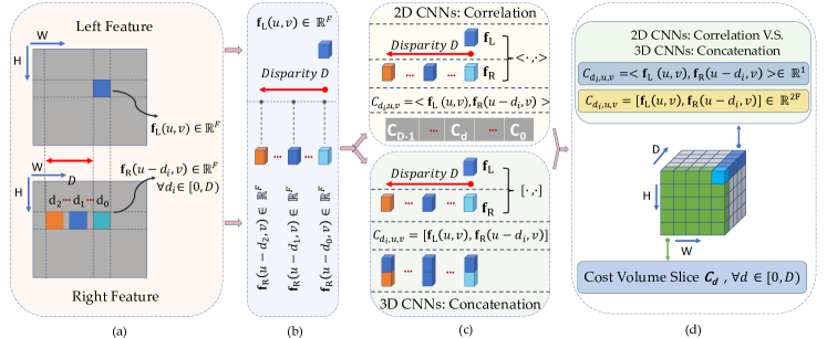
Figure 1: Cost volume in 2D and 3D CNNs for stereo matching. (a) Deep features are extracted for each view. (b) A left feature vector $\mathbf{f}_{L}(u,v)$ and several counterparts $\mathbf{f}_{R}(u-d_{i},v)$, at disparity $d_{i}\in[0,D)$. (c) The left feature vector is either correlated (top branch for 2D CNNs) or concatenated (bottom branch for 3D CNNs) with the corresponding right feature vectors. (d) The cost volume, including the highlighted cost volume slice $\mathcal{C}_{d}$ (green), cost volume fiber $\mathcal{C}_{u,v}$ (blue) and cost feature $\mathcal{C}_{d,u,v}$ (light blue) that is a scalar for 2D CNNs or a vector for 3D CNNs.

Given a rectified stereo pair $\mathbf{I}_{L}$ and $\mathbf{I}_{R}$ with dimensions $H\times W$ ($H$: height, $W$: width), stereo matching finds the correspondence between a reference pixel $\mathbf{p}_{L}$ in the left image $\mathbf{I}_{L}$ and a target pixel $\mathbf{p}_{R}$ in the right image $\mathbf{I}_{R}$. The cost volume (or matching volume) $\mathcal{C}$ is defined as a 3D or 4D tensor with dimensions $D\times H\times W$ or $2F\times D\times H\times W$ ($D$: disparity range, $F$: feature dimensionality for each of the views), to represent the likelihood of a reference pixel $\mathbf{p}_{L}(u,v)$ corresponding to a target pixel $\mathbf{p}_{R}(u-d,v)$, with disparity $d\in[0,D)$. Its construction is illustrated in Fig 1. Specifically, the extracted left feature vector $\mathbf{f}_{L}(u,v)\in\mathbb{R}^{F}$ of the reference pixel $\mathbf{p}_{L}(u,v)$ is either correlated (in 2D CNNs e.g. DispNetC [29] and iResNet [26]) or concatenated (in 3D CNNs e.g. GCNet [23], PSMNet [7] and GANet [45]) with the corresponding feature $\mathbf{f}_{R}(u-d,v)\in\mathbb{R}^{F}$ of the target pixel $\mathbf{p}_{R}(u-d,v)$, for each disparity $d\in\{0,\dots,D-1\}$. It is formulated in Eq. 1:

$$\mathcal{C}_{d,u,v}=\begin{cases}\langle\mathbf{f}_{L}(u,v),\mathbf{f}_{R}(u-d,y)\rangle\in\mathbb{R}^{1}&\text{\small{2D CNNs}}\\ [\mathbf{f}_{L}(u,v),\mathbf{f}_{R}(u-d,v)]\in\mathbb{R}^{2F}&\text{\small{3D CNNs}}\\ \end{cases}$$ (1)

where $\langle\cdot,\cdot\rangle$ denotes correlation, $[\cdot,\cdot]$ indicates concatenation, resulting in a 3D or 4D tensor for 2D and 3D CNNs, respectively. We denote a cost volume slice at disparity $d$ by $\mathcal{C}_{d}$ (i.e., $\mathcal{C}_{d}=\mathcal{C}_{d,u,v}|_{u=1:W;v=1:H}$).

3.2 Content-Adaptive Filtering Modules

In this subsection, we present four content-adaptive filtering approaches which can be effectively incorporated as content-adaptive CNN layers in state-of-the-art networks for end-to-end stereo matching.

3.2.1 Segmentation-aware Bilateral Filtering Module

Segmentation-aware bilateral filtering (SABF) [17] was proposed to enforce smoothness while preserving region boundaries or motion discontinuities in dense prediction tasks, such as semantic segmentation and optical flow estimation. As shown in Fig. 2, here we adapt the SABF to stereo matching to filter the cost volume $\mathcal{C}$ (Sec. 3.1), by (i) learning to embed in a feature space where semantic dissimilarity between pixels can be measured by a distance function [10]; (ii) creating local foreground (relative to a given pixel) attention filters $K^{sabf}$; (iii) filtering the cost volume $\mathcal{C}$ so as to capture the relevant foreground and be robust to appearance variations in the background or occlusions.

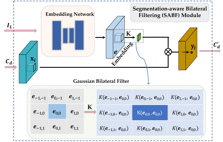
Figure 2: Integrating the segmentation-aware bilateral filtering (SABF) module. The upper branch shows the embedding $\mathbf{e}$ is learned by an embedding network from an input image $\mathbf{I}_{L}$. Pairwise embedding distances are converted (Eq. 4) to SABF filter weights $K$, as shown at the bottom. The overall figure shows how SABF filters a cost volume slice $\mathcal{C}_{d}$ to obtain a segmentation-aware filtered result $\mathcal{C}^{\prime}_{d}$.

Learning the Embedding.   Given an RGB image $\mathbf{I}$, consisting of $N$ pixels $\mathbf{q}$, and its semantic segmentation label map $\mathbf{l}$, the embedding function is implemented as an Embedding Network (see the detailed architecture in supplement) that maps pixels into an embedding space as $f:\mathbb{R}^{3}\mapsto\mathbb{R}^{64}$, or $f(\mathbf{q})=\mathbf{e}$, where $\mathbf{e}\in\mathbb{R}^{64}$ is the embedding for RGB pixel $\mathbf{q}$, with $64$ as the dimension of the embedding space. See Fig. 2. The embeddings are learned via a loss function over pixel pairs sampled in a neighborhood around each pixel. Specifically, for any two pixels $\mathbf{p}_{i}$ and $\mathbf{p}_{j}$ and corresponding object class labels $\mathbf{l}_{i}$ and $\mathbf{l}_{j}$, the pairwise loss is:

$$\ell_{i,j}=\begin{cases}\text{ }\max(||\mathbf{e}_{i}-\mathbf{e}_{j}||_{1}-\alpha,0)&\text{if }\mathbf{l}_{i}=\mathbf{l}_{j}\\ \text{ }\max(\beta-||\mathbf{e}_{i}-\mathbf{e}_{j}||_{1},0)&\text{if }\mathbf{l}_{i}\neq\mathbf{l}_{j}\\ \end{cases}$$ (2)

where $||\cdot||_{1}$ indicates the $L_{1}$-norm, and the thresholds are $\alpha=0.5$ and $\beta=2$. Therefore, the total loss for all the pixels in the image $\mathbf{I}$ is defined in Eq. 3:

$$\mathcal{L}=\sum_{i=0}^{N-1}\sum_{j\in\mathcal{N}_{i}}\ell_{i,j}$$ (3)

where $j\in\mathcal{N}_{i}$ spans the spatial neighbors of index $i$. We follow the implementation of Harley et al. [17] where three overlapping $3\times 3$ neighborhoods with dilation rates of $1$, $2$, and $5$ are used for a good trade-off between long-range pairwise connectivity and computational efficiency.

Applying the SABF Layer.   Once the embedding is learned, the SABF filter weights are obtained by converting the pairwise distance between $\mathbf{e}_{i}$ and $\mathbf{e}_{j}$ into (unnormalized) probabilities using two Gaussian distributions as in Eq. 4:

$$K^{sabf}_{i,j}=\exp{\left(-\frac{||\mathbf{p}_{i}-\mathbf{p}_{j}||^{2}}{2\sigma_{s}^{2}}-\frac{||\mathbf{e}_{i}-\mathbf{e}_{j}||^{2}}{2\sigma_{r}^{2}}\right)}$$ (4)

where $\sigma_{s}$ and $\sigma_{r}$ are two predefined standard deviations. Then, given an input feature $\mathbf{x}_{i}$, we can efficiently compute a segmentation-aware filtered result $\mathbf{y}_{i}$ via the SABF layer:

$$\mathbf{y}_{i}=\frac{\sum_{k\in\Omega(i)}\mathbf{x}_{k}\,K^{sabf}_{i,k}}{\sum_{k\in\Omega(i)}K^{sabf}_{i,k}}$$ (5)

where $\Omega(\cdot)$ defines an $s\times s$ (e.g., $5\times 5$) filtering window. The input $\mathbf{x}_{i}$ and output $\mathbf{y}_{i}$ here are from a raw cost volume slice $\mathcal{C}_{d}$ and the filtered slice $\mathcal{C}^{\prime}_{d}$, respectively (Fig. 2).

3.2.2 Dynamic Filtering Networks (DFN) Module

Dynamic Filter Networks (DFN) [22] are a content-adaptive filtering technique. As shown in Fig. 4(b), the filters $\mathcal{F}_{\theta}$ in the DFN are dynamically generated by a separate filter-generating network conditioned on an input $\textbf{x}_{A}$. Then, they are applied to another input $\mathbf{x}_{B}$ via the dynamic filtering layer. In our implementation, $\mathbf{x}_{A}$ is the deep feature $\mathbf{f}_{L}$ of the reference image $\mathbf{I}_{L}$, and $\mathbf{x}_{B}$ is a cost volume slice $\mathcal{C}_{d}$.

Filter-Generating Network.   Given an input $\mathbf{x}_{A}\in\mathbb{R}^{H\times W\times C_{A}}$ ($H$: height, $W$: width, $C_{A}$: channel size of $\mathbf{x}_{A}$), the filter-generating network generates dynamic filters $\mathcal{F}_{\theta}$, parameterized by $\theta\in\mathbb{R}^{s\times s\times C_{B}\times n_{F}}$ ($s$: filter window size, $C_{B}$: channel size of $\mathbf{x}_{B}$, $n_{F}$: the number of filters).

Dynamic Local Filtering Layer.   The generated filters $\mathcal{F}_{\theta}$ are applied to input images or feature maps $\mathbf{x}_{B}\in\mathbb{R}^{H\times W\times C_{B}}$ via the dynamic filtering layer to output the filtered result $G=\mathcal{F}_{\theta}(\mathbf{x}_{B})\in\mathbb{R}^{H\times W}$. Specifically, the dynamic filtering layer in the DFN [22] has two types of instances: dynamic convolutional layer (with $n_{F}=1$) and dynamic local filtering layer (with $n_{F}=H\cdot W$). The latter is adopted in this paper because it guarantees content-adaptive filtering via applying a specific local filter $\mathcal{F}_{\theta}^{(u,v)}$ to the neighborhood centered around each pixel coordinate $(u,v)$ of the input $\mathbf{x}_{B}$:

$$G(u,v)=\mathcal{F}_{\theta}^{(u,v)}(\mathbf{x}_{B}(u,v))$$ (6)

Therefore, the operations in Eq. 6 are not only input content specific but also spatial position specific.

3.2.3 Pixel Adaptive Convolutional (PAC) Module

Pixel adaptive convolution (PAC) proposed by Su et al. [34] is a new content-adaptive convolution, which can alleviate the drawback of standard convolution that ignores local image content, while retaining its favorable spatial sharing property compared with existing content-adaptive filters, e.g. the DFN [22]. As illustrated in Fig. 4(a), PAC modifies a conventional spatially invariant convolution filter $\mathbf{W}$ at each position by multiplying it with a position-specific filter $K^{pac}$, the adapting kernel. $K^{pac}$ has a pre-defined form, e.g. Gaussian: $e^{-\frac{1}{2}||\mathbf{f}_{i}-\mathbf{f}_{j}||^{2}}$, where $\mathbf{f}_{i}$ and $\mathbf{f}_{j}$ are the adapting features, corresponding to pixels $\mathbf{p}_{i}$ and $\mathbf{p}_{j}$. The adapting features $\mathbf{f}$ can be either hand-crafted (e.g. position and color features) or deep features. We use deep features extracted from the left image as the adapting features $\mathbf{f}$.

Given an input $\mathbf{x}_{i}\in\mathbb{R}^{C_{x}}$ at pixel $\mathbf{p}_{i}$, the output $\mathbf{y}_{i}\in\mathbb{R}^{C_{y}}$ filtered by PAC is defined as

$$\mathbf{y}_{i}=\sum_{j\in\Omega(i)}\,K^{pac}{(\mathbf{f}_{i},\mathbf{f}_{j})}\,\mathbf{W}{[\mathbf{p}_{i}-\mathbf{p}_{j}]}\,\mathbf{x}_{i}\,+\mathbf{b}$$ (7)

where $C_{x}$ and $C_{y}$ denote the feature dimension of $\mathbf{x}_{i}$ and $\mathbf{y}_{i}$, respectively. $\Omega(\cdot)$ defines an $s\times s$ convolution window. $\mathbf{W}\in\mathbb{R}^{C_{y}\times C_{x}\times s\times s}$ and $\mathbf{b}\in\mathbb{R}^{C_{y}}$ indicate the convolution filter weights and biases. We adopt the notation $[\mathbf{p}_{i}-\mathbf{p}_{j}]$ to spatially index filter weights $\mathbf{W}$ with 2D spatial offsets. In our approach $\mathbf{x}_{i}$ and $\mathbf{y}_{i}$ are from the raw and filtered cost volume slices $\mathcal{C}_{d}$ and $\mathcal{C}^{\prime}_{d}$, respectively.

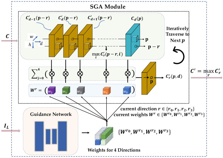
Figure 3: Integrating the SGA module. The bottom branch shows the guidance network which generates aggregation weights in four directions. The top branch illustrates SGA which iteratively aggregates the cost volume $\mathcal{C}$ via traversing from pixel $\mathbf{p}-\mathbf{r}$ to $\mathbf{p}$ in a direction $\mathbf{r}$, over the entire image and each disparity $d$. The maximum response among the four directions is selected as the output $\mathcal{C}^{\prime}$.

3.2.4 Semi-Global Aggregation Module

In contrast to the above filters that leverage local context, Semi-Global Aggregation (SGA) [45] is able to iteratively aggregate the cost volume considering both pixelwise costs and pairwise smoothness constraints in four directions. The constraints are originally defined and approximately solved by Semi-Global Matching (SGM) [20] as an energy function of the disparity map. SGA learns to aggregate the cost volume $\mathcal{C}$ to approximately minimize the energy, and also support backpropagation for end-to-end stereo matching as shown in Fig. 3. The aggregated cost volume $\mathcal{C}^{\prime}$ is recursively defined as:

$$\begin{split}\mathcal{C}^{\prime}_{\mathbf{r}}(\mathbf{p},d)&=\text{sum }\begin{cases}\mathbf{w}_{0}(\mathbf{p},\mathbf{r})\cdot\mathcal{C}(\mathbf{p},d)\\ \mathbf{w}_{1}(\mathbf{p},\mathbf{r})\cdot\mathcal{C}^{\prime}_{\mathbf{r}}(\mathbf{p}-\mathbf{r},d)\\ \mathbf{w}_{2}(\mathbf{p},\mathbf{r})\cdot\mathcal{C}^{\prime}_{\mathbf{r}}(\mathbf{p}-\mathbf{r},d-1)\\ \mathbf{w}_{3}(\mathbf{p},\mathbf{r})\cdot\mathcal{C}^{\prime}_{\mathbf{r}}(\mathbf{p}-\mathbf{r},d+1)\\ \mathbf{w}_{4}(\mathbf{p},\mathbf{r})\cdot\underset{i}{\mathrm{max}}\,\,\mathcal{C}^{\prime}_{\mathbf{r}}(\mathbf{p}-\mathbf{r},i)\\ \end{cases}\end{split}$$ (8)

where $\mathbf{r}$ is a unit direction vector along which the cost $\mathcal{C}^{\prime}_{\mathbf{r}}(\mathbf{p},d)$ of pixel $\mathbf{p}$ at disparity $d$ is aggregated. The weights $\mathbf{w}_{j}$ are achieved and normalized (s.t. $\sum_{j=0}^{4}\mathbf{w}_{j}(\mathbf{p},\mathbf{r})=1$) by a guidance sub-network to avoid very large accumulated values when traversing along the path. The final aggregated cost $\mathcal{C}^{\prime}_{\mathbf{r}}(\mathbf{p},d)$ is obtained by picking the maximum among four directions, namely, left, right, up and down, i.e., $\mathbf{r}\in\{(-1,0),(1,0),(0,1),(0,-1)\}$, defined as:

$$\mathcal{C}^{\prime}(\mathbf{p},d)=\underset{\mathbf{r}}{\mathrm{max}}\,\,\mathcal{C}^{\prime}_{\mathbf{r}}(\mathbf{p},d)$$ (9)

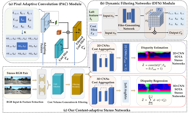
Figure 4: (a) PAC filters the cost volume slice $\mathcal{C}_{d}$ by multiplying it with a standard spatially invariant convolutional filter $\mathbf{W}$ and a spatially varying filter $K$ that depends on input pixel features $\mathbf{f}$. The output is the filtered slice $\mathcal{C}^{\prime}_{d}$. (b) DFN filters $\mathcal{F}_{\theta}$ are dynamically generated by the filter-generating network conditioned on left pixel features $\mathbf{f}_{L}$. $\mathcal{C}_{d}$ is filtered by $\mathcal{F}_{\theta}$ to output $\mathcal{C}^{\prime}_{d}$. (c) Overview of network architecture: a stereo pair is fed into a weight-sharing Siamese sub-network for feature learning; the extracted features of each view are correlated or concatenated to generate the cost volume $\mathcal{C}$; content-adaptive filtering modules are applied to $\mathcal{C}$ and output the filtered volume $\mathcal{C}^{\prime}_{d}$, followed by state-of-the-art encoder-decoder cost aggregation and disparity regression, as shown in two branches for 2D and 3D convolutional architectures.

3.3 Network Architecture

As illustrated in Fig. 4, our architecture takes as backbones four state-of-the-art 2D and 3D CNNs for stereo matching, i.e., DispNetC [29], GCNet [23], PSMNet [7] and GANet [45], and adapts SABF (Fig. 2), PAC (Fig. 4(a)), DFN (Fig. 4(b)) and SGA (Fig. 3), to aggregate the cost volume.

3.3.1 Network Backbones

Given a rectified stereo pair, the backbone architectures described below include unary feature extraction from the images by a weight-sharing Siamese structure, cost volume computation and regularization, and disparity regression. Unary features are denoted by $\mathbf{f}_{u}$. 2D or 3D convolutional and transpose convolutional layers have $3\times 3$ or $3\times 3\times 3$ kernels, unless otherwise specified.

DispNetC Backbone.   DispNetC [29] is an encoder-decoder architecture with an explicit 1D correlation layer. The encoder downsamples the input images via convolution by up to $1/64$, while the decoder gradually upsamples the feature maps via transposed convolution at 6 different scales ranging from $1/64$ to $1/2$. Features $\mathbf{f}_{u}$ ($H/4\times W/4\times F$, $F=128$) are correlated by a 1D correlation layer [13] to form a 3D cost volume $\mathcal{C}$ ($D/4\times H/4\times W/4$) with a maximum disparity of $D/4$. $\mathcal{C}$ is further contracted to $1/64$ resolution and expanded by alternate transpose convolutions and loss layers. There are six intermediate disparity maps which are all interpolated to the input resolution. The loss is computed on all six disparity maps, but only the last one is used as output.

GCNet Backbone.   GCNet [23] is a 3D CNN architecture that models geometry in stereo matching. We add an initial bilinear interpolation layer to downsample the input stereo pair to half resolution. GCNet extracts $\mathbf{f}_{u}$ ($F\times H/4\times W/4$, $F=32$) via a $5\times 5$ convolution layer and eight residual blocks [19] and then builds a 4D cost volume $\mathcal{C}$ ($D/4\times 2F\times H/4\times W/4$) by concatenating $\mathbf{f}_{u}$ with its counterpart from the other view across each disparity level. $\mathcal{C}$ is downsampled by up to $1/16$ via four encoding blocks (each with three convolutions with strides equal to $2$, $1$, and $1$) and upsampled by $32$ via five decoding blocks (each has a skip-connection from the early layer and one transposed convolution with stride $2$), resulting in an aggregated ($D/2\times H/2\times W/2$) volume. It is interpolated to input resolution and regressed to predict the disparity map via the differentiable soft argmin:

$$\hat{\mathcal{D}}=\sum_{d=0}^{D-1}d\cdot\sigma(-\mathcal{C}_{d})$$ (10)

where cost $\mathcal{C}_{d}$ is first converted to a probability of each disparity value $d$ via the softmax operation $\mathbf{\sigma}(\cdot)$.The disparity map $\hat{\mathcal{D}}$ comprises the expected values of $d$ for each pixel.

PSMNet Backbone.   PSMNet [7] learns $\mathbf{f}_{u}$ ($F\times H/4\times W/4$, $F=128$) via three convolution layers followed by four basic residual blocks [19]. $\mathbf{f}_{u}$ is further processed separately by spatial pyramid pooling (SPP), a $1\times 1$ convolution, bilinear interpolation and feature concatenation. This generates the SPP features ($F\times H/4\times W/4$, $F=32$) used to construct a 4D ($D/4\times 2F\times H/4\times W/4$) cost volume $\mathcal{C}$. $\mathcal{C}$ is regularized by a stacked hourglass with three encoding-decoding blocks. Each hourglass generates a regularized volume, from which an intermediate disparity is obtained via the soft argmin (Eq. 10). The training loss is computed on all three intermediate disparities.

GANet Backbone.   GANet [45] introduces local guided aggregation (LGA) and semi-global aggregation (SGA) layers which are complementary to 3D convolutional layers. The unary features $\mathbf{f}_{u}$ ($F\times H/3\times W/3$, $F=32$) are extracted through a stacked hourglass CNN with skip connections. They are then used to construct a 4D cost volume ($D/3\times 2F\times H/3\times W/3$), which is fed into a cost aggregation block (built of alternate 3D convolution and transpose convolution layers, SGA and LGA) for regularization, refinement and disparity regression via the soft argmin (Eq. 10). The guidance sub-network generates the weight matrices for SGA (Sec. 3.2) and LGA. The LGA layer is used before disparity regression and locally refines the 4D cost volume for several times. We adopt the GANet-deep version which achieves the best accuracy among all variants.

Network Capacity.  Network capacities are listed in Table 1. The parameters of four backbone networks (i.e, row W/O in gray, meaning no filters applied) increase in the order of GCNet $<$ PSMNet $<$ GANet $<$ DispNetC. The order of the filtering modules (rows in skyblue) according to increasing number of parameters is PAC $<$ DFN $<$ SABF $<$ SGA.

3.3.2 Loss Function

The smooth $L_{1}$ loss function (see the supplement) is used for end-to-end training. The GCNet backbone has one disparity output, while the other backbones produce multiple intermediate disparity maps. The network loss is their weighted average. The corresponding weights are defined as 1) GANet: $0.2$, $0.6$, and $1.0$; 2) PSMNet: $0.5$, $0.7$, and $1.0$; 3) DispNetC: $0.05$, $0.10$, $0.14$, $0.19$, $0.24$, and $0.29$ as training starts on Scene Flow, while in finetuning, only the final disparity is activated. When integrating the SABF filter to the backbones, the embedding loss in Eq. 3 is added with a weight of $0.06$.

Filters	Network Backbones
	DispNetC		PSMNet		GANet		GCNet
	No.	$\uparrow$(%)	No.	$\uparrow$(%)	No.	$\uparrow$(%)	No.	$\uparrow$(%)
mygrayW/O	42.2	-	5.2	-	6.6	-	2.8	-
myskyblueSABF	44.0	4.2	7.0	34	8.4	27	4.6	62.4
myskyblueDFN	42.6	0.8	5.6	6.4	6.9	5.1	3.2	11.8
myskybluePAC	42.3	0.1	5.3	2.0	6.7	1.6	2.9	3.6
myskyblueSGA	45.2	7.0	8.3	58.8	-	-	5.9	108

Table 1: Network capacity. For each combination of the filtering techniques and network backbones, columns No. show the number of parameters in millions, and columns $\uparrow$(%) are the relative increase in the number of parameter w.r.t. the backbone baselines. Largest values are in bold. Inapplicable entries are marked by “-”.

4 Experiments

4.1 Datasets

Our networks are trained from scratch on Scene Flow [29], then finetuned on Virtual KITTI 2 (VKT2) [5, 15] or KITTI 2015 (KT15) [30]. Scene Flow is a large scale synthetic dataset containing $35,454$ training and $4,370$ testing images with dense ground truth disparity maps. We exclude the pixels with disparities $d>192$ in training. Virtual KITTI 2 (VKT2) is a synthetic clone of the real KITTI dataset. It contains 5 sequence clones of Scene 01, 02, 06, 18 and 20, and nine variants with diverse weather conditions (e.g. fog, rain) or modified camera configurations (e.g. rotated by $15\degree$, $30\degree$). Since there is no designated validation set, we select (i) Scene06 (i.e., VKT2-Val-S6 with $2,700$ frames) and (ii) multiple blocks of consecutive frames from Scene 01, 02, 18, 20 (i.e., VKT2-Val-WoS6 with $2,620$ frames), and use the remaining $15,940$ images for training. The former scene remains unseen during training, while networks observe similar frames to the latter. We evaluate these settings separately. KITTI 2015 (KT15): is a real dataset of street views. It contains $200$ training stereo image pairs with sparsely labeled disparity from LiDAR data. We divided the training data into a training set ($170$ images) and a validation set ($30$ images) for our experiments.

Metrics.   For KT15, we adopt the bad-3 error (i.e., percentage of pixels with disparity error $>3$px or $\geq 5\%$ of the true disparity) counted over non-occluded (noc) or all pixels with ground truth. For VKT2, in addition to bad-3, we also use the endpoint error (EPE) and bad-1 error ($\geq 1$px or $\geq 5\%$) over all pixels.

Filters	DispNetC			PSMNet			GANet			GCNet
	EPE(px)	$\geq 1$ px	$\geq 3$ px	EPE(px)	$\geq 1$ px	$\geq 3$ px	EPE(px)	$\geq 1$ px	$\geq 3$ px	EPE(px)	$\geq 1$ px	$\geq 3$ px
Seen locations (i.e., Scene01, 02, 18 and 20) from VKT2 validation set VKT2-Val-WoS6
W/O	0.68	11.54	3.72	0.45	7.08	2.21	0.33	5.34	1.70	0.62	9.71	3.18
myskyblueSABF	mygray0.65	mygray 10.86	mygray 3.48	mygray0.36	mygray5.92	mygray1.98	0.34	5.50	1.76	mygray0.60	9.89	3.19
myskyblue DFN	mygray 0.57	mygray9.85	mygray3.26	mygray0.42	mygray6.45	mygray2.17	0.37	6.23	1.99	mygray0.60	mygray9.20	mygray3.11
myskybluePAC	mygray0.58	mygray9.92	mygray3.39	0.52	7.81	2.61	0.40	7.01	2.20	0.75	12.98	4.02
myskyblueSGA	mygray0.57	mygray9.37	mygray3.21	mygray0.40	mygray6.08	mygray2.14	-	-	-	mygray0.55	mygray9.24	mygray2.98
Totally unseen location (i.e., Scene06) from VKT2 validation set VKT2-Val-S6
W/O	0.70	10.28	3.12	0.48	5.16	1.96	0.30	3.09	1.0563	0.59	7.48	2.25
myskyblueSABF	mygray0.69	mygray 9.75	mygray 3.00	mygray0.44	mygray4.47	mygray1.73	mygray0.28	3.16	mygray0.97	mygray0.56	7.51	mygray2.23
myskyblue DFN	mygray 0.599	mygray8.54	mygray2.791	mygray0.39	mygray4.83	mygray1.69	mygray0.29	3.54	mygray 1.0561	mygray0.55	mygray6.81	mygray2.14
myskybluePAC	mygray0.603	mygray8.73	mygray2.96	0.52	5.78	1.98	0.35	4.36	1.47	0.73	11.87	2.99
myskyblueSGA	mygray0.607	mygray8.02	mygray2.794	mygray0.42	mygray4.34	mygray1.71	-	-	-	mygray0.53	mygray7.45	2.29

Table 2: Evaluation on the validation sets of VKT2-Val-WoS6 and VKT2-Val-S6. Results are shown in the entries of filters (rows in skyblue) and backbones (columns) w.r.t. the baselines (rows W/O). Our improved results are highlighted in gray, and the best ones are in bold. GANet already contains SGA, resulting in blank entries “-”.

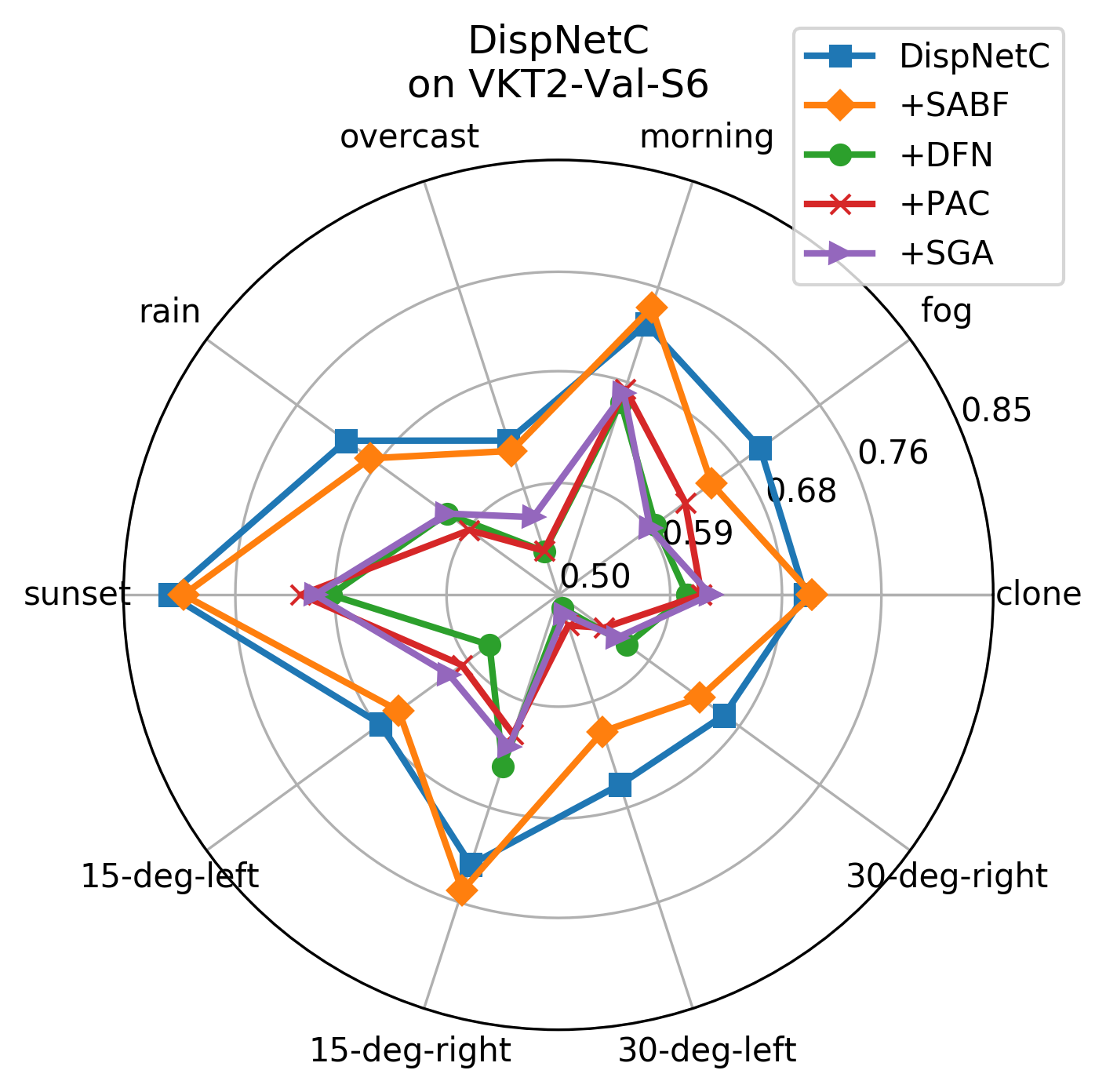
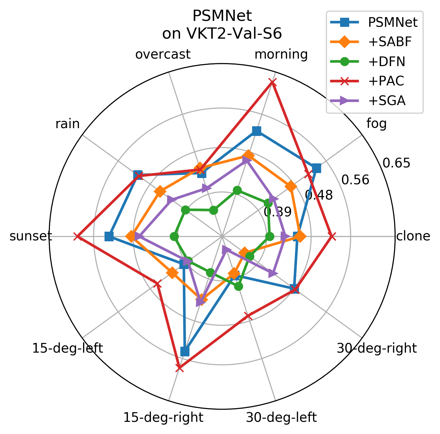
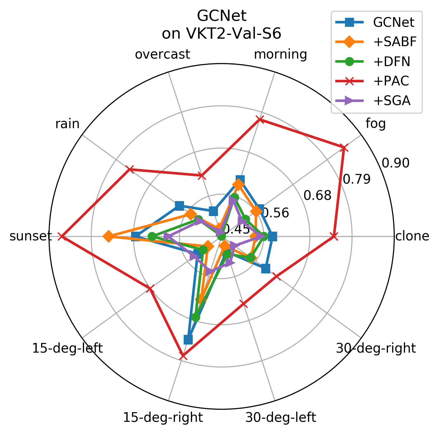
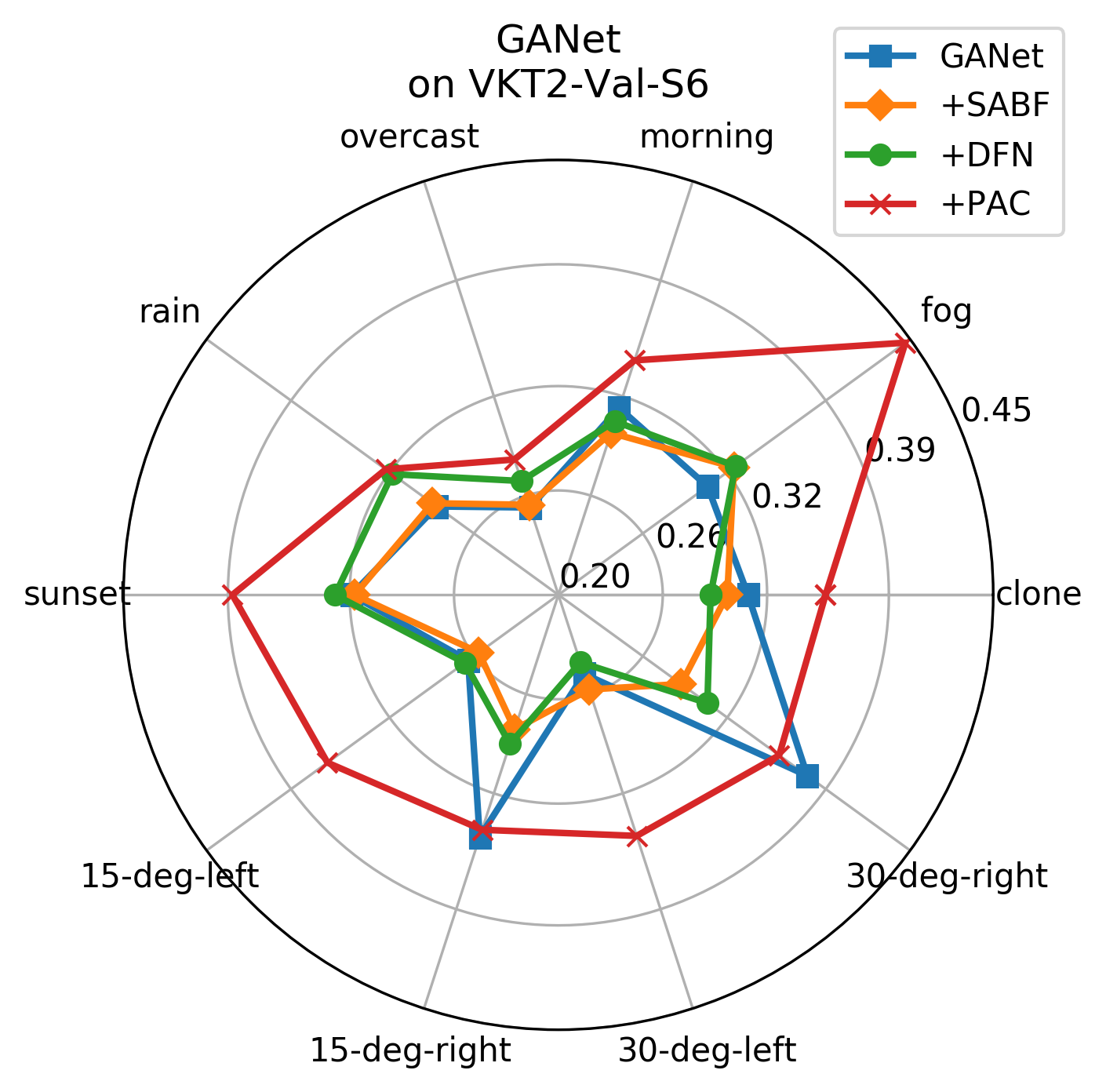
(a)	(b)	(c)	(d)

Figure 5: Results of (a) DispNetC, (b) PSMNet, (c) GCNet and (d) GANet on each category of validation set VKT2-Val-S6.

4.2 Implementation Details

Architecture Details.   Our models are implemented with PyTorch. Each convolution layer is followed by batch normalization (BN) and ReLU unless otherwise specified. We use the official code of PSMNet and GANet, and implement DispNetC (no PyTorch version) and GCNet (no official code). Our implementations achieve similar or better results on the KT15 benchmark, i.e., bad-3 errors $4.48\%$ (all) and $3.85\%$ (noc) versus the authors’ $4.34\%$ (all) and $4.05\%$ (noc) for DispNetC, and $2.38\%$ (all) and $2.07\%$ (noc) versus the authors’ $2.87\%$ (all) and $2.61\%$ (noc) for GCNet. We use $\sigma_{s}=0.7$ and $\sigma_{r}=0.1$ in Eq. 4 for SABF. We investigate how the filter window $s$ and dilation rate $r$ affect the filtering output, and find that $s=5$ with $r=2$ achieve a good balance in accuracy, space requirements and runtime. Please see the supplementary material for ablation studies.

Training Details.   The SABF embedding network is pre-trained on Cityscapes [11]. For data augmentation we randomly crop $256\times 512$ image patches and do channel-wise standardization by subtracting the mean and dividing by the standard deviation. For fair comparison, we follow the baselines and set the maximum disparity to $D=192$. We use the official pre-trained models on Scene Flow for GANet and PSMNet, and train DispNetC and GCNet on Scene Flow from scratch for $10$ epochs with a learning rate (lr) of $0.001$. Training is optimized with Adam ($\beta_{1}=0.9$, $\beta_{2}=0.999$), except for GCNet which uses RMSprop ($\alpha=0.9$). For KT15, our models and baselines are finetuned for 600 epochs (with lr of 0.001 for the first $300$ epochs and 0.0001 for the next $300$ epochs). For VKT2, we finetune all algorithms for $20$ epochs, with lr of 0.001 at first, then divided by 10 at epoch 5 and epoch 18.

4.3 Quantitative Results

All the results are on the validation sets since we could not submit all combinations to the benchmarks. Due to page limits, qualitative results are available in the supplement.

Virtual KITTI 2 Evaluation.  We finetune our models (the pre-trained backbones on Scene Flow after integrating the filters) on the VKT2 dataset. (EPE, bad-1 and bad-3) on the VKT2-Val-WoS6 and VKT2-Val-S6 validation sets are listed in Table 2. In most cases, our models (rows in skyblue) achieve higher accuracy than the baselines (row W/O). The exception is standard GANet which performs well since it always includes SGA and LGA for global and local matching volume aggregation. Fig. 5 plots EPE errors on individual categories of VKT2-Val-S6. SABF, DFN and SGA boost 2D and 3D CNNs, while PAC improves 2D CNNs, but not 3D CNNs. When moving from familiar (VKT2-Val-WoS6) to unseen (VKT2-Val-S6) validation scenes, DFN achieves better adaptation than SGA, and the SABF and DFN variants outperform standard GANet.

KITTI 2015 Evaluation.  The results on KT15 are shown in Table 3. Our networks obtain improved accuracy for all the backbones except for GANet. All the filters boost the backbones due to leveraging image context as guidance, and SGA achieves the highest accuracy among them.

Filters	DispNetC		PSMNet		GANet		GCNet
	noc	all	noc	all	noc	all	noc	all
W/O	2.59	3.02	1.46	1.60	0.97	1.10	2.06	2.64
myskyblue SABF	mygray2.26	mygray2.63	mygray1.28	mygray1.40	1.07	1.17	mygray1.76	mygray 2.10
myskyblue DFN	mygray 2.37	mygray 2.78	mygray 1.23	mygray 1.34	0.99	1.11	mygray 1.70	mygray 2.08
myskyblue PAC	mygray 2.38	mygray 2.72	mygray 1.29	mygray 1.48	1.13	1.23	mygray 1.71	mygray 2.03
myskyblue SGA	mygray1.90	mygray2.18	mygray1.17	mygray1.32	-	-	mygray1.69	mygray1.91

Table 3: KITTI 2015 bad-3 validation results. Improved results are highlighted in gray, and best ones are in bold. GANet contains SGA, resulting in blank entries “-”.

Runtime   In Table 4, we compare the GPU memory consumption and runtime in inference mode on pairs of frames with dimension $384\times 1280$. All experiments are run on the same machine, with the same configuration of disparity range $D=192$, filter size $s=5$ and dilation rate $r=2$.

Comparison and Summary.   Our results show that most architectures benefit from adaptive filtering, with the exception of GANet, which already includes such filtering of SGA. It is worth pointing that GANet has the largest number of parameters and the longest runtime among the backbones. Lighter architectures, e.g. PSMNet+SABF or PSMNet+DFN can achieve competitive results. DispNetC trails in terms of accuracy, but has about 20% of the footprint of GANet and its combination with DFN strikes a good balance between accuracy and processing requirements.

5 Conclusions

We demonstrate how deep adaptive or guided filtering can be integrated into representative 2D and 3D CNNs for stereo matching with improved accuracy. Our extensive experimental results on Virtual KITTI 2 and KITTI 2015 highlight how our filtering modules effectively leverage the RGB information to dynamically guide the matching, resulting in further progress in stereo matching. SGA, a component of GANet, is the most effective filtering mechanism and improves all backbones. More broadly, our work shows that current state-of-the-art methods do not take full advantage of available information, with the exception of GANet which shows superior performance due to SGA and LGA, but has more parameters than GCNet and PSMNet. Integrating even the smaller filtering modules leads to decreases in error in the order of 10%.

Filters	DispNetC		PSMNet		GANet		GCNet
	Mem.	Time	Mem.	Time	Mem.	Time	Mem.	Time
W/O	1394	18.35	5151	315.57	7178	1894.70	4280	146.83
myskyblue SABF	1888	24.32	5386	563.42	7920	2488.72	4424	379.37
myskyblue DFN	1422	28.33	5246	432.32	7466	2041.53	4298	255.20
myskybluePAC	1535	25.34	5168	514.91	8274	2383.44	4400	334.73
myskyblue SGA	7066	489.60	11070	823.00	-	-	9916	655.18

Table 4: Runtime (ms) and GPU memory consumption (MiB). Results are shown in the entries of filters (rows in skyblue) and backbones (columns) w.r.t. the baselines (rows W/O). The smallest values are in bold. GANet already contains SGA, resulting in blank entries “-”.

Acknowledgements.   This research has been partially supported by National Science Foundation under Awards IIS-1527294 and IIS-1637761.

Supplement

In this supplementary material, we show the loss function, more details of filtering modules in the network, ablation study, and additional qualitative results, some of which are mentioned but not fully discussed in the main paper due to the page limit.

Loss Function.   The loss is evaluated over the valid pixels which have ground truth disparity. We adopt the smooth $L_{1}$ loss function for end-to-end training:

$$L(d,\hat{d}) =\frac{1}{N}\sum_{i=1}^{N}l_{s}(||d_{i}-\hat{d_{i}}||_{1})$$ (11)

$$\text{and, }l_{s}(x) =\begin{cases}0.5x^{2}&\text{if }|x|<1\\ |x|-0.5&\text{otherwise}\end{cases}$$

where $N$ counts the valid pixels, $||d_{i}-\hat{d_{i}}||_{1}$ measures the absolute error of disparity prediction $\hat{d_{i}}$ and ground truth $d_{i}$.

Deep Adaptive Filtering Architectures.   The integrated deep adaptive or guided filters include segmentation-aware bilateral filtering (SABF) [17], dynamic filtering networks (DFN) [22], pixel adaptive convolution (PAC) [34] and semi-global aggregation (SGA). Please see our source code (https://github.com/ccj5351/DAFStereoNets) for the detailed architectures. Fig. 6 shows the embedding network of SABF.

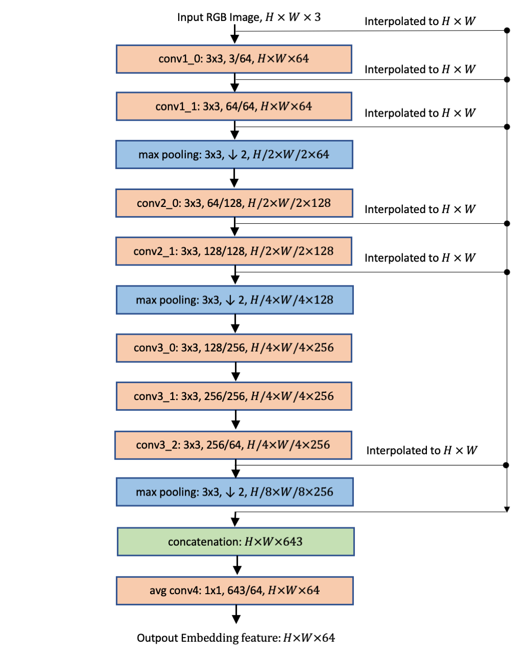
Figure 6: The embedding network in the segmentation-aware bilateral filtering (SABF) module. Each convolutional layer is followed by a ReLU layer which is not drawn. Convolutional layers, e.g. conv1_0, are defined by $3\times 3$ as filter, $3/64$ as in/out feature planes, and $H\times W\times 64$ as the output dimension). Max pooling layers are implemented as $3\times 3$ filter with stride of $2$ for downsampling (i.e., $\downarrow 2$).

Ablation Study.    We perform ablation studies to investigate how the filter window $s$ and the dilation rate $r$ can affect the filtering output and disparity estimation. Out of a large number of possible combinations, we show two representatives DispNetC+SABF and PSMNet+SABF in Table 5. We find that $s=5$ with $r=2$ achieve a good balance in accuracy, space and runtime. The 500-run averaged memory consumption and runtime in GPUs are measured when we test a $384\times 1280$ stereo pair, and the bad-3 (noc,all) errors are evaluated on the KITTI 2015 validation set. Please note that a $5\times 5$ filter (with dilation rate $2$) covers $9\times 9$ regions in the cost feature space, which is equivalent to $33\times 33$ regions in the RGB image space, due to the cost volume being a quarter of the size of the input images. In the following experiments, we keep using $s=5$ with $r=2$ for our different architectures. Please note that the results in Table 5 are obtained on a 16-core Intel Core i7-9800X CPU at 3.80GHz, and an NVIDIA TITAN Xp GPU with 12GB of RAM.

Effectiveness Comparison    In Table 7, we further investigate the effectiveness among those variants in terms of parameter increase (column $\delta P$%) and error decrease (column $\delta E$%) evaluated on the KITTI 2015 validation set, as shown in Table 6. Please note that Table 6 is originally included in the main paper, and we repeat it here to explain the effectiveness in Table 7.

filter size $s$	DispNetC+SABF						PSMNet+SABF
	$r=1$		$r=2$		Mem.	Time	$r=1$		$r=2$		Mem.	Time
	EPE(px)	$\geq$3(%)	EPE(px)	$\geq$3(%)	(MiB)	(ms)	EPE(px)	$\geq$3(%)	EPE(px)	$\geq$3(%)	(MiB)	(ms)
$s=3$	0.875	3.14	0.845	2.99	2132	45.26	0.639	1.63	0.643	1.61	4681	449.40
$s=5$	0.867	3.13	mygray 0.841	mygray 2.90	mygray 2228	mygray 48.99	0.657	1.54	mygray 0.630	mygray 1.46	mygray 4989	mygray 633.42
$s=7$	0.832	2.83	0.795	2.46	2588	54.21	0.650	1.50	0.642	1.54	4709	939.40
$s=9$	0.825	2.84	0.854	3.00	3008	60.56	0.868	1.77	0.689	1.91	4953	1226.72

Table 5: Illustration of the effects of different filter window sizes $s$ and dilation rates $r$. We computer the bad-3 (noc,all) errors on the KITTI 2015 validation set and the averaged GPU memory consumption and runtime to test a pair of frames with dimension $384\times 1280$.

Filters	DispNetC		PSMNet		GANet		GCNet
	noc	all	noc	all	noc	all	noc	all
W/O	2.59	3.02	1.46	1.60	0.97	1.10	2.06	2.64
myskyblue SABF	mygray2.26	mygray2.63	mygray1.28	mygray1.40	1.07	1.17	mygray1.76	mygray 2.10
myskyblue DFN	mygray 2.37	mygray 2.78	mygray 1.23	mygray 1.34	0.99	1.11	mygray 1.70	mygray 2.08
myskyblue PAC	mygray 2.38	mygray 2.72	mygray 1.29	mygray 1.48	1.13	1.23	mygray 1.71	mygray 2.03
myskyblue SGA	mygray1.90	mygray2.18	mygray1.17	mygray1.32	-	-	mygray1.69	mygray1.91

Table 6: KITTI 2015 bad-3 validation results. Improved results are highlighted in gray, and best ones are in bold. GANet contains SGA, resulting in blank entries “-”.

Filters	DispNetC		PSMNet		GANet		GCNet
	$\delta$E(%)	$\delta$P(%)	$\delta$E(%)	$\delta$P(%)	$\delta$E(%)	$\delta$P(%)	$\delta$E(%)	$\delta$P(%)
SABF	12.9	4.2	12.4	34	-5.9	27	20.6	62.4
DFN	7.9	0.8	16.2	6.4	-0.1	5.1	21.5	11.8
PAC	9.9	0.1	7.8	2.0	-12	1.6	23.3	3.6
SGA	27.8	7.0	17.7	58.8	-	-	27.7	108

Table 7: Effectiveness comparison on the KITTI 2015 val-30 dataset. For each combination of network backbone and filtering, columns $\delta$E(%) and $\delta$P(%) indicate the relative decrease of error and increase of the number of parameters, respectively, w.r.t. the backbone baselines.

Qualitative Results    In Figs. 7–10, we show reference images and disparity maps generated by each backbone without modifications and the same backbone after integrating one of the filtering techniques.

	\begin{overpic}[width=163.96347pt]{img/dispnetc-disp-color-0045.png} \put(85.0,25.0){$\displaystyle{\color[rgb]{1,1,1}\textbf{7.19\%}}$} \put(75.0,17.0){{\color[rgb]{1,1,1} \circle{18.0}}} \end{overpic}	\begin{overpic}[width=163.96347pt]{img/pac-dispnetc-disp-color-0045.png} \put(85.0,25.0){$\displaystyle{\color[rgb]{1,1,1}\textbf{4.66\%}}$} \put(75.0,17.0){{\color[rgb]{1,1,1} \circle{18.0}}} \end{overpic}
	\begin{overpic}[width=163.96347pt]{img/dispnetc-disp-color-1880.png} \put(85.0,25.0){$\displaystyle{\color[rgb]{1,1,1}\textbf{3.03\%}}$} \put(6.0,6.0){{\color[rgb]{1,1,1} \circle{12.0}}} \end{overpic}	\begin{overpic}[width=163.96347pt]{img/pac-dispnetc-disp-color-1880.png} \put(85.0,25.0){$\displaystyle{\color[rgb]{1,1,1}\textbf{2.43\%}}$} \put(6.0,6.0){{\color[rgb]{1,1,1} \circle{12.0}}} \end{overpic}
	(a)
	\begin{overpic}[width=163.96347pt]{img/dispnetc-disp-color-0001-000005_10.png} \put(85.0,23.0){$\displaystyle{\color[rgb]{1,1,1}\textbf{7.59\%}}$} \put(13.0,17.0){{\color[rgb]{1,1,1} \circle{12.0}}} \end{overpic}	\begin{overpic}[width=163.96347pt]{img/sabf-dispnetc-disp-color-0001-000005_10.png} \put(85.0,23.0){$\displaystyle{\color[rgb]{1,1,1}\textbf{5.42\%}}$} \put(13.0,17.0){{\color[rgb]{1,1,1} \circle{12.0}}} \end{overpic}
	\begin{overpic}[width=163.96347pt]{img/dispnetc-disp-color-0011-000086_10.png} \put(5.0,20.0){$\displaystyle{\color[rgb]{1,1,1}\textbf{9.23\%}}$} \put(88.0,15.0){{\color[rgb]{1,1,1} \circle{22.0}}} \end{overpic}	\begin{overpic}[width=163.96347pt]{img/sabf-dispnetc-disp-color-0011-000086_10.png} \put(5.0,20.0){$\displaystyle{\color[rgb]{1,1,1}\textbf{7.35\%}}$} \put(88.0,15.0){{\color[rgb]{1,1,1} \circle{22.0}}} \end{overpic}
	(b)

Figure 7: Results using DispNetC as backbone. (a) DispNetC vs DispNetC+PAC on Virtual KITTI 2 Scene06 validation set. (b) DispNetC vs DispNetC+SABF on KITTI 2015 validation set. In all rows, the left image is the reference image of the stereo pair, the middle column in the disparity map from the unmodified backbone, and the right image is the disparity map of the backbone with the integrated filter.

	\begin{overpic}[width=163.96347pt]{img/gcnet-disp-color-0125.png} \put(4.0,25.0){$\displaystyle{\color[rgb]{1,1,1}\textbf{3.84\%}}$} \put(75.0,17.0){{\color[rgb]{1,1,1} \circle{18.0}}} \end{overpic}	\begin{overpic}[width=163.96347pt]{img/sga-gcnet-disp-color-0125.png} \put(4.0,25.0){$\displaystyle{\color[rgb]{1,1,1}\textbf{2.03\%}}$} \put(75.0,17.0){{\color[rgb]{1,1,1} \circle{18.0}}} \end{overpic}
	\begin{overpic}[width=163.96347pt]{img/gcnet-disp-color-2535.png} \put(4.0,25.0){$\displaystyle{\color[rgb]{1,1,1}\textbf{11.50\%}}$} \put(90.0,19.0){{\color[rgb]{1,1,1} \circle{18.0}}} \end{overpic}	\begin{overpic}[width=163.96347pt]{img/sga-gcnet-disp-color-2535.png} \put(4.0,25.0){$\displaystyle{\color[rgb]{1,1,1}\textbf{6.69\%}}$} \put(90.0,19.0){{\color[rgb]{1,1,1} \circle{18.0}}} \end{overpic}
	(a)
	\begin{overpic}[width=163.96347pt]{img/gcnet-disp-color-0001-000005_10.png} \put(4.0,25.0){$\displaystyle{\color[rgb]{1,1,1}\textbf{6.94\%}}$} \put(53.0,24.0){{\color[rgb]{1,1,1} \circle{15.0}}} \end{overpic}	\begin{overpic}[width=163.96347pt]{img/sga-gcnet-disp-color-0001-000005_10.png} \put(4.0,25.0){$\displaystyle{\color[rgb]{1,1,1}\textbf{4.82\%}}$} \put(53.0,24.0){{\color[rgb]{1,1,1} \circle{15.0}}} \end{overpic}
	\begin{overpic}[width=163.96347pt]{img/gcnet-disp-color-0022-000131_10.png} \put(4.0,25.0){$\displaystyle{\color[rgb]{1,1,1}\textbf{4.03\%}}$} \put(50.0,24.0){{\color[rgb]{1,1,1} \circle{15.0}}} \end{overpic}	\begin{overpic}[width=163.96347pt]{img/sga-gcnet-disp-color-0022-000131_10.png} \put(4.0,25.0){$\displaystyle{\color[rgb]{1,1,1}\textbf{2.54\%}}$} \put(50.0,24.0){{\color[rgb]{1,1,1} \circle{15.0}}} \end{overpic}
	(b)

Figure 8: Results using GCNet as backbone. (a) GCNet vs GCNet+SGA on Virtual KITTI 2 Scene06 validation set. (b) GCNet vs GCNet+SGA on KITTI 2015 validation set. In all rows, the left image is the reference image of the stereo pair, the middle column in the disparity map from the unmodified backbone, and the right image is the disparity map of the backbone with the integrated filter.

	\begin{overpic}[width=163.96347pt]{img/psm-disp-color-1615.png} \put(2.0,25.0){$\displaystyle{\color[rgb]{1,1,1}\textbf{4.71\%}}$} \put(87.0,17.0){{\color[rgb]{1,1,1} \circle{18.0}}} \end{overpic}	\begin{overpic}[width=163.96347pt]{img/dfn-psm-disp-color-1615.png} \put(2.0,25.0){$\displaystyle{\color[rgb]{1,1,1}\textbf{2.70\%}}$} \put(87.0,17.0){{\color[rgb]{1,1,1} \circle{18.0}}} \end{overpic}
	\begin{overpic}[width=163.96347pt]{img/psm-disp-color-2535.png} \put(2.0,25.0){$\displaystyle{\color[rgb]{1,1,1}\textbf{12.23\%}}$} \put(90.0,17.0){{\color[rgb]{1,1,1} \circle{18.0}}} \end{overpic}	\begin{overpic}[width=163.96347pt]{img/dfn-psm-disp-color-2535.png} \put(2.0,25.0){$\displaystyle{\color[rgb]{1,1,1}\textbf{3.81\%}}$} \put(90.0,17.0){{\color[rgb]{1,1,1} \circle{18.0}}} \end{overpic}
	(a)
	\begin{overpic}[width=163.96347pt]{img/psm-disp-color-0017-000114_10.png} \put(2.0,25.0){$\displaystyle{\color[rgb]{1,1,1}\textbf{2.29\%}}$} \put(50.0,16.0){{\color[rgb]{1,1,1} \circle{10.0}}} \put(55.0,8.0){{\color[rgb]{1,1,1} \circle{12.0}}} \end{overpic}	\begin{overpic}[width=163.96347pt]{img/pac-psm-disp-color-0017-000114_10.png} \put(2.0,25.0){$\displaystyle{\color[rgb]{1,1,1}\textbf{1.21\%}}$} \put(50.0,16.0){{\color[rgb]{1,1,1} \circle{10.0}}} \put(55.0,8.0){{\color[rgb]{1,1,1} \circle{12.0}}} \end{overpic}
	\begin{overpic}[width=163.96347pt]{img/psm-disp-color-0023-000173_10.png} \put(2.0,25.0){$\displaystyle{\color[rgb]{1,1,1}\textbf{3.02\%}}$} \put(8.0,8.0){{\color[rgb]{1,1,1} \circle{14.0}}} \end{overpic}	\begin{overpic}[width=163.96347pt]{img/pac-psm-disp-color-0023-000173_10.png} \put(2.0,25.0){$\displaystyle{\color[rgb]{1,1,1}\textbf{1.71\%}}$} \put(8.0,8.0){{\color[rgb]{1,1,1} \circle{14.0}}} \end{overpic}
	(b)

Figure 9: Results using PSMNet as backbone. (a) PSMNet vs PSMNet+DFN on Virtual KITTI 2 Scene06 validation set.(b) PSMNet vs PSMNet+PAC on KITTI 2015 validation set. In all rows, the left image is the reference image of the stereo pair, the middle column in the disparity map from the unmodified backbone, and the right image is the disparity map of the backbone with the integrated filter.

	\begin{overpic}[width=163.96347pt]{img/ganet-disp-color-2640.png} \put(2.0,25.0){$\displaystyle{\color[rgb]{1,1,1}\textbf{6.34\%}}$} \put(54.0,15.0){{\color[rgb]{1,1,1} \circle{20.0}}} \end{overpic}	\begin{overpic}[width=163.96347pt]{img/sabf-ganet-disp-color-2640.png} \put(2.0,25.0){$\displaystyle{\color[rgb]{1,1,1}\textbf{2.33\%}}$} \put(54.0,15.0){{\color[rgb]{1,1,1} \circle{20.0}}} \end{overpic}
	\begin{overpic}[width=163.96347pt]{img/ganet-disp-color-1495.png} \put(2.0,25.0){$\displaystyle{\color[rgb]{1,1,1}\textbf{4.30\%}}$} \put(93.0,15.0){{\color[rgb]{1,1,1} \circle{12.0}}} \end{overpic}	\begin{overpic}[width=163.96347pt]{img/sabf-ganet-disp-color-1495.png} \put(2.0,25.0){$\displaystyle{\color[rgb]{1,1,1}\textbf{1.22\%}}$} \put(93.0,15.0){{\color[rgb]{1,1,1} \circle{12.0}}} \end{overpic}
	(a)
	\begin{overpic}[width=163.96347pt]{img/ganet-disp-color-0019-000122_10.png} \put(2.0,25.0){$\displaystyle{\color[rgb]{1,1,1}\textbf{1.79\%}}$} \put(7.0,16.0){{\color[rgb]{1,1,1} \circle{12.0}}} \end{overpic}	\begin{overpic}[width=163.96347pt]{img/pac-ganet-disp-color-0019-000122_10.png} \put(2.0,25.0){$\displaystyle{\color[rgb]{1,1,1}\textbf{1.12\%}}$} \put(7.0,16.0){{\color[rgb]{1,1,1} \circle{12.0}}} \end{overpic}
	\begin{overpic}[width=163.96347pt]{img/ganet-disp-color-0029-000196_10.png} \put(10.0,25.0){$\displaystyle{\color[rgb]{1,1,1}\textbf{1.07\%}}$} \put(5.0,20.0){{\color[rgb]{1,1,1} \circle{10.0}}} \end{overpic}	\begin{overpic}[width=163.96347pt]{img/pac-ganet-disp-color-0029-000196_10.png} \put(10.0,25.0){$\displaystyle{\color[rgb]{1,1,1}\textbf{0.95\%}}$} \put(5.0,20.0){{\color[rgb]{1,1,1} \circle{10.0}}} \end{overpic}
	(b)

Figure 10: Results using GANet as backbone. (a) GANet vs GANet+SABF on Virtual KITTI 2 Scene06 validation set. (b) GANet vs GANet+PAC on KITTI 2015 validation set. In all rows, the left image is the reference image of the stereo pair, the middle column in the disparity map from the unmodified backbone, and the right image is the disparity map of the backbone with the integrated filter.

References

- [1] V. Aurich and J. Weule. Non-linear Gaussian filters performing edge preserving diffusion. In Mustererkennung 1995, pages 538–545. Springer, 1995.
- [2] S. P. Awate and R. T. Whitaker. Higher-order image statistics for unsupervised, information-theoretic, adaptive, image filtering. In CVPR, volume 2, pages 44–51. IEEE, 2005.
- [3] S. Bako, T. Vogels, B. McWilliams, M. Meyer, J. Novák, A. Harvill, P. Sen, T. Derose, and F. Rousselle. Kernel-predicting convolutional networks for denoising monte carlo renderings. ACM Trans. Graph., 36(4):97–1, 2017.
- [4] A. Buades, B. Coll, and J.-M. Morel. A non-local algorithm for image denoising. In CVPR, volume 2, pages 60–65, 2005.
- [5] Y. Cabon, N. Murray, and M. Humenberger. Virtual KITTI 2. arXiv preprint arXiv:2001.10773, 2020.
- [6] S. Chandra and I. Kokkinos. Fast, exact and multi-scale inference for semantic image segmentation with deep Gaussian CRFs. In ECCV, pages 402–418, 2016.
- [7] J.-R. Chang and Y.-S. Chen. Pyramid stereo matching network. In CVPR, pages 5410–5418, 2018.
- [8] L.-C. Chen, J. T. Barron, G. Papandreou, K. Murphy, and A. L. Yuille. Semantic image segmentation with task-specific edge detection using cnns and a discriminatively trained domain transform. In CVPR, pages 4545–4554, 2016.
- [9] L.-C. Chen, A. Schwing, A. Yuille, and R. Urtasun. Learning deep structured models. In ICML, pages 1785–1794, 2015.
- [10] S. Chopra, R. Hadsell, and Y. LeCun. Learning a similarity metric discriminatively, with application to face verification. In CVPR, pages 539–546, 2005.
- [11] M. Cordts, M. Omran, S. Ramos, T. Rehfeld, M. Enzweiler, R. Benenson, U. Franke, S. Roth, and B. Schiele. The cityscapes dataset for semantic urban scene understanding. In CVPR, pages 3213–3223, 2016.
- [12] J. Dai, H. Qi, Y. Xiong, Y. Li, G. Zhang, H. Hu, and Y. Wei. Deformable convolutional networks. In ICCV, Oct 2017.
- [13] A. Dosovitskiy, P. Fischer, E. Ilg, P. Hausser, C. Hazirbas, V. Golkov, P. Van Der Smagt, D. Cremers, and T. Brox. Flownet: Learning optical flow with convolutional networks. In ICCV, pages 2758–2766, 2015.
- [14] R. Gadde, V. Jampani, M. Kiefel, D. Kappler, and P. Gehler. Superpixel convolutional networks using bilateral inceptions. In ECCV, pages 597–613. Springer, 2016.
- [15] A. Gaidon, Q. Wang, Y. Cabon, and E. Vig. Virtual worlds as proxy for multi-object tracking analysis. In Proceedings of the IEEE conference on Computer Vision and Pattern Recognition, pages 4340–4349, 2016.
- [16] X. Guo, K. Yang, W. Yang, X. Wang, and H. Li. Group-wise correlation stereo network. In CVPR, 2019.
- [17] A. W. Harley, K. G. Derpanis, and I. Kokkinos. Segmentation-aware convolutional networks using local attention masks. In ICCV, pages 5038–5047, 2017.
- [18] K. He, J. Sun, and X. Tang. Guided image filtering. PAMI, 35(6):1397–1409, 2012.
- [19] K. He, X. Zhang, S. Ren, and J. Sun. Deep residual learning for image recognition. In CVPR, pages 770–778, 2016.
- [20] H. Hirschmüller. Stereo processing by semiglobal matching and mutual information. PAMI, 30(2):328–341, 2008.
- [21] V. Jampani, M. Kiefel, and P. V. Gehler. Learning sparse high dimensional filters: Image filtering, dense crfs and bilateral neural networks. In CVPR, pages 4452–4461, 2016.
- [22] X. Jia, B. De Brabandere, T. Tuytelaars, and L. V. Gool. Dynamic filter networks. In Advances in Neural Information Processing Systems, pages 667–675, 2016.
- [23] A. Kendall, H. Martirosyan, S. Dasgupta, P. Henry, R. Kennedy, A. Bachrach, and A. Bry. End-to-end learning of geometry and context for deep stereo regression. In ICCV, pages 66–75, 2017.
- [24] P. Krähenbühl and V. Koltun. Efficient inference in fully connected crfs with Gaussian edge potentials. In NIPS, pages 109–117, 2011.
- [25] Y. Li, J.-B. Huang, A. Narendra, and M.-H. Yang. Deep joint image filtering. In ECCV, pages 154–169, 2016.
- [26] Z. Liang, Y. Feng, Y. Guo, H. Liu, W. Chen, L. Qiao, L. Zhou, and J. Zhang. Learning for disparity estimation through feature constancy. In CVPR, pages 2811–2820, 2018.
- [27] G. Lin, C. Shen, A. Van Den Hengel, and I. Reid. Efficient piecewise training of deep structured models for semantic segmentation. In CVPR, pages 3194–3203, 2016.
- [28] S. Liu, S. De Mello, J. Gu, G. Zhong, M.-H. Yang, and J. Kautz. Learning affinity via spatial propagation networks. In NIPS, pages 1520–1530, 2017.
- [29] N. Mayer, E. Ilg, P. Hausser, P. Fischer, D. Cremers, A. Dosovitskiy, and T. Brox. A large dataset to train convolutional networks for disparity, optical flow, and scene flow estimation. In CVPR, pages 4040–4048, 2016.
- [30] M. Menze and A. Geiger. Object scene flow for autonomous vehicles. In CVPR, pages 3061–3070, 2015.
- [31] J. Pang, W. Sun, J. S. Ren, C. Yang, and Q. Yan. Cascade residual learning: A two-stage convolutional neural network for stereo matching. In ICCV Workshop on Geometry Meets Deep Learning, Oct 2017.
- [32] D. Scharstein and R. Szeliski. A taxonomy and evaluation of dense two-frame stereo correspondence algorithms. IJCV, 47(1-3):7–42, 2002.
- [33] X. Song, X. Zhao, L. Fang, and H. Hu. EdgeStereo: An effective multi-task learning network for stereo matching and edge detection. IJCV, 2020.
- [34] H. Su, V. Jampani, D. Sun, O. Gallo, E. Learned-Miller, and J. Kautz. Pixel-adaptive convolutional neural networks. In CVPR, 2019.
- [35] C. Tomasi and R. Manduchi. Bilateral filtering for gray and color images. In Sixth international conference on computer vision (IEEE Cat. No. 98CH36271), pages 839–846. IEEE, 1998.
- [36] A. Tonioni, F. Tosi, M. Poggi, S. Mattoccia, and L. Di Stefano. Real-time self-adaptive deep stereo. In CVPR, June 2019.
- [37] X. Wang, R. Girshick, A. Gupta, and K. He. Non-local neural networks. In CVPR, pages 7794–7803, 2018.
- [38] H. Wu, S. Zheng, J. Zhang, and K. Huang. Fast end-to-end trainable guided filter. In CVPR, pages 1838–1847, 2018.
- [39] J. Wu, D. Li, Y. Yang, C. Bajaj, and X. Ji. Dynamic filtering with large sampling field for convnets. In The European Conference on Computer Vision (ECCV), September 2018.
- [40] T. Xue, J. Wu, K. Bouman, and B. Freeman. Visual dynamics: Probabilistic future frame synthesis via cross convolutional networks. In NIPS, pages 91–99, 2016.
- [41] G. Yang, H. Zhao, J. Shi, Z. Deng, and J. Jia. SegStereo: Exploiting semantic information for disparity estimation. In ECCV, pages 636–651, 2018.
- [42] Z. Yin, T. Darrell, and F. Yu. Hierarchical discrete distribution decomposition for match density estimation. In CVPR, June 2019.
- [43] J. Žbontar and Y. LeCun. Stereo matching by training a convolutional neural network to compare image patches. Journal of Machine Learning Research, 17(1-32):2, 2016.
- [44] W. Zhan, X. Ou, Y. Yang, and L. Chen. DSNet: Joint learning for scene segmentation and disparity estimation. In IEEE International Conference on Robotics and Automation, pages 2946–2952, 2019.
- [45] F. Zhang, V. Prisacariu, R. Yang, and P. H. Torr. Ga-net: Guided aggregation net for end-to-end stereo matching. In CVPR, 2019.
- [46] S. Zheng, S. Jayasumana, B. Romera-Paredes, V. Vineet, Z. Su, D. Du, C. Huang, and P. H. S. Torr. Conditional random fields as recurrent neural networks. In ICCV, 2015.
- [47] X. Zhu, H. Hu, S. Lin, and J. Dai. Deformable convnets v2: More deformable, better results. In CVPR, June 2019.