Matching-space Stereo Networks for Cross-domain Generalization

Abstract

End-to-end deep networks represent the state of the art for stereo matching. While excelling on images framing environments similar to the training set, major drops in accuracy occur in unseen domains (e.g., when moving from synthetic to real scenes). In this paper we introduce a novel family of architectures, namely Matching-Space Networks (MS-Nets), with improved generalization properties. By replacing learning-based feature extraction from image RGB values with matching functions and confidence measures from conventional wisdom, we move the learning process from the color space to the Matching Space, avoiding over-specialization to domain specific features. Extensive experimental results on four real datasets highlight that our proposal leads to superior generalization to unseen environments over conventional deep architectures, keeping accuracy on the source domain almost unaltered. Our code is available at https://github.com/ccj5351/MS-Nets.

1 Introduction

The rising availability of stereo imagery with ground truth depth [8, 23, 29, 32] has enabled the development of machine learning based stereo matching algorithms. The first attempts to exploit machine learning for dense correspondence focused on matching [1, 7, 20, 45] or other stages [2, 9, 26, 27, 33] of the stereo pipeline [30] and were combined with conventional components. As in other areas of computer vision, end-to-end methods [21] soon became the dominant paradigm. They can be distinguished in two categories according to network architecture: 2D [19, 21, 24, 35, 42] and 3D [5, 17, 44, 46] convolutional networks. The latter reason about geometry by building a matching volume, either correlating or concatenating learned features from the images. 3D convolutions enable these methods to consider context beyond a fixed disparity value (a slice of the matching volume) for higher accuracy.

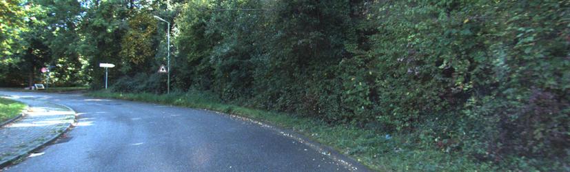
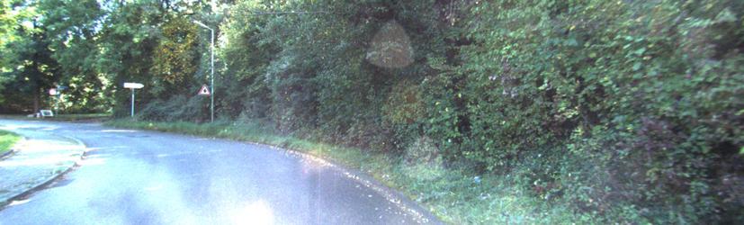
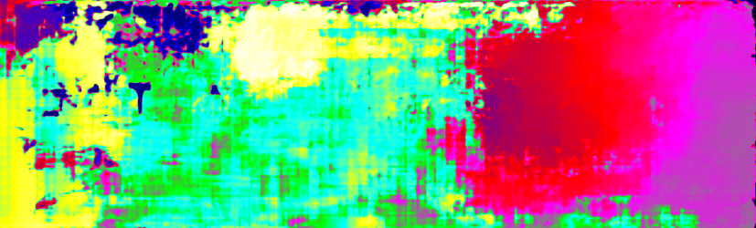
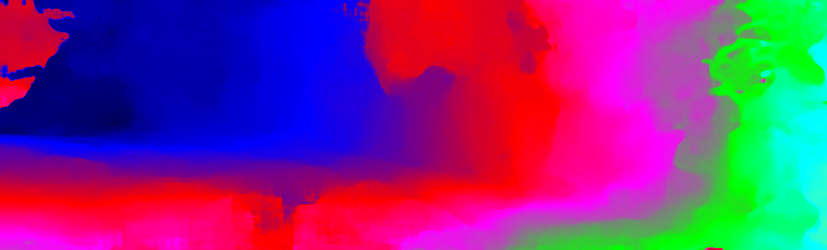
(a)	(b)	(c)	(d)

Figure 1: Generalization across domains. (a) and (b) Challenging stereo pair from the KITTI dataset. (c) Disparity map estimated by PSMNet [5]. (d) Disparity map estimated by our MS-PSMNet. Both networks are trained on the same synthetic data.

Although end-to-end models excel at specializing on specific domains when enough data are available for training, e.g. autonomous driving [8, 23], they are less effective at generalization to very different domains or with high variety of image content. Strong evidence supporting this emerges by browsing online benchmarks: while on KITTI 2012 [8] and 2015 [23] end-to-end networks dominate the leaderboards, very few of them appear on the Middlebury 2014 leaderboard [29] and typically achieve lower accuracy than hand-designed algorithms [36] deploying machine learning on individual steps [45] of the pipeline. This is due to the diversity of the Middlebury dataset.

Poor generalization is a cause for concern, since gathering annotated data may be too expensive or infeasible in practical applications. We argue that this lack of generalization, or over-specialization, is caused by the learning process being driven by image content, i.e. the network learns how to match pixels by strongly relying on appearance properties. When such content differs substantially from the one observed in training, end-to-end approaches suffer large accuracy drops. Usually large amounts of labelled images, often generated in synthetic environments [21], are used to improve generalization and mitigate this effect. On the other hand, domain shifts still pose difficulties [25, 37, 40], in particular when moving from synthetic to real imagery affected by reflective surfaces, sensor noise and illumination conditions, which have not been modeled in the simulators. Anyway, there is evidence in literature that this effect can be soften by moving the learning process to different representations [1] or parts of the pipeline [31]. We claim that better generalization can be achieved by choosing a representation insensitive to common variations of the input images. Instead of augmenting the dataset to guide the network to achieve certain invariances, one could design a hybrid approach in which some invariances are learned from the data while others are imposed by the design. For example, if we wish the network to be invariant to affine transformations of image intensity or color, we would use normalized cross correlation (NCC) in a conventional stereo algorithm. In an end-to-end trainable algorithm, we could either achieve this invariance via augmenting the data by affinely transforming one of the images, or by using an NCC-like abstraction in the representation of the images.

In this paper, we propose a new family of end-to-end architectures designed to have invariant properties that make them robust to domain shifts. Our networks learn to reason about stereo matching in the domain of matching functions by combining four matching functions and associated confidence scores [15, 28]. Stacking multiple of these cues results in a 4D tensor compatible with matching volumes processed by 3D networks. This way, the network is never exposed to image appearance and is forced to learn in the Matching Space (MS) only, avoiding over-specialization.

We demonstrate the effectiveness of the proposed representation by implementing two 3D convolutional architectures based on the above principle. Specifically, we replicate two popular, but different, 3D convolutional networks, GCNet [17] and PSMNet [5], replacing their matching volume, which is based on deep image features, with the proposed MS representation. Extensive experiments show that our MS-Nets generalize better to data from domains that differ substantially from the training one. We believe that the reason for this is that our approach learns to reason on relationships in the matching volume without being affected by image appearance, which our networks never observe directly. Figure 1 shows disparity estimation by both PSMNet and its MS variant on a challenging stereo pair from KITTI, after being trained on synthetic images only. In particular, we can notice large changes of illumination between the two frames, possibly never observed during training. Estimated disparity maps show that such perturbations drive PSMNet to totally unreliable estimations. Conversely, MS-PSMNet learned a robust representation leading to accurate results.

Our claim is supported by extensive experimental results on five popular datasets: SceneFlow [21], KITTI 2012 [8], KITTI 2015 [23], Middlebury 2014 [29] and ETH3D [32]. In particular, we study a variety of training protocols involving both large and limited amounts of labelled images in order to dig deeper into the relationship between training data and model performance, an aspect that has been largely ignored in previous works [5, 17, 19, 21, 35, 42]. Our MS-Nets are able to generalize much better than GCNet and PSMNet with minor loss of accuracy in the source domain. The main contributions of this paper are:

• The observation and testing of the hypothesis that not exposing CNNs directly to image appearance leads to better generalization properties;

• A novel family of architectures, MS-Nets, and one of its possible implementations built on conventional wisdom [1] and popular 3D networks [17, 5];

• An extensive set of experiments highlighting the behavior of both 3D and MS-Nets under domain shift.

2 Related Work

The problem of disparity estimation from stereo image pairs has been studied for decades. We refer readers to survey papers [8, 16, 28, 30]. In this section, we review deep learning based stereo methods, broadly divided into matching cost learning and optimization and end-to-end dense disparity regression.

Matching cost learning and optimization.   Convolutional Neural Networks for predicting the matching costs were first introduced by [45]. The outputs of the MC-CNN network were refined according to the non-learned traditional pipeline [22, 30] to generate disparity maps. [20] substituted an inner product layer for the fully connected layer in MC-CNN [45] to alleviate the expensive computational burden. [34] presented a network for matching cost computation, utilizing a highway network with multi-level weighted residual shortcuts. A deep embedding model presented by [7] was learned from a multi-scale ensemble framework, which fuses feature vectors learned at different scales. [33] used CNNs to learn the penalty-parameters of the Semi-Global Matching (SGM) algorithm [13] and proposed a new parameterization of the same algorithm discriminating between positive and negative disparity changes. In contrast, our method, combining conventional matching functions and confidence measures as matching cost, can be trained end-to-end.

End-to-end disparity regression.   Mayer et al. [21] were the first to propose an end-to-end stereo network, namely DispNet, with an encoder-decoder architecture for disparity estimation trained on a large synthetic dataset created by them. This synthetic dataset enabled the development of end-to-end deep stereo networks. [17] presented GCNet to exploit contextual information for disparity regression, via 3D-convolution on the matching volume using deep unary features and a differentiable soft-argmin operation. Chang and Chen put forward PSMNet [5] consisting of spatial pyramid pooling for unary feature extraction, and stacked 3D hourglasses for matching volume regularization. StereoDRNet [4] extends PSMNet [5] by replacing the spatial pyramid pooling [12] with vortex pooling [41] in feature extraction, and by utilizing 3D dilated convolutions in cost volume filtering. [44] learned cost aggregation via a two-stream network for generation and selection of cost aggregation proposals. In parallel, more architectures built on DispNet have been proposed, leveraging cascade residual learning [24] or deploying multi-task learning by jointly learning disparity estimation together with edge detection [35] or semantic segmentation [42]. [19] incorporated matching cost calculation and aggregation, disparity estimation and refinement into one network, ranking first at the Robust Vision Challenge 2018. [11] constructed the matching volume by group-wise correlation of features which were split into multiple groups along the channel dimension. Zhang et al. [46] proposed GA-Net, a deep guided aggregation network, including semi-global aggregation (SGA) and local guided aggregation (LGA) layers for efficient end-to-end stereo matching. Our proposed networks, never exposed to RGB values, are trained end-to-end from the matching space to final disparity maps.

Deep learning for domain transfer.   Most deep stereo models are particularly data dependent and their performance drops considerably when dealing with unseen domains different from those observed during training [37, 38]. To tackle the domain shift problem, two main strategies are involved: image synthesis [6, 14, 18], and un-/self-supervised adaptation [3, 10, 25, 37, 38, 39, 40, 48, 49]. In contrast, our method aims at being transferred without adaptation to different domains, being this possibility more appealing for practical applications.

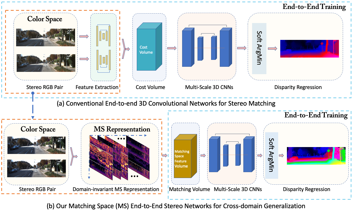
Figure 2: Architecture overview. (a) shows a conventional end-to-end 3D convolutional network for stereo matching. (b) illustrates our end-to-end MS-Nets architecture. The orange dashed boxes show the different feature extractors of the two architectures. The blue dashed boxes show the part of each network that is trained end-to-end. Feature extractors in MS-Nets are fixed and isolate the network from RGB.

3 Approach

Deep learning methods [5, 17, 21, 45, 48] work extremely well on disparity estimation when sufficient data with ground truth are available. However, they have been proven vulnerable to out-of-distribution data. When dealing with unseen environments quite different from those employed to train the network, the accuracy may rapidly decrease. By moving the learning process to Matching Space, we force the neural network to learn a more general representation, avoiding over-fitting to specific image appearance statistics that are characteristic of the training domain and thus to be more robust to such decreases.

For one possible implementation of MS-Nets, we select a subset of the CBMV features [1], which have shown good generalization across distinct datasets with respect to neural networks [45] when used to learn a matching function. In contrast to existing end-to-end networks, which are directly exposed to raw image intensities (or RGB values) [5, 17, 21, 45, 48], the proposed MS-Nets, leveraging features that encode geometric constraints and prior knowledge, can be transferred without adaptation to different domains. The general architecture of the proposed family of networks is shown in Fig. 2.

As base architectures, we have chosen PSMNet [5] and GCNet [17]. Both belong to the 3D CNN category, but they have different architectures and parameter configuration. Specifically, PSMNet has 3.3M ($63.5\%$) parameters in the unary feature extraction modules, versus only 1.9M ($36.5\%$) in the 3D CNN layers for cost volume regularization. On the other hand, GCNet has the opposite configuration, i.e. 0.3M ($11.5\%$) parameters for feature extraction and 2.3M ($88.5\%$) parameters in the 3D CNNs. We will show how these differences impact generalization.

3.1 Matching-Space Features and Volume

We follow the notation of [1] in this section. Given a rectified stereo pair comprising the left and right image, $I_{L}$ and $I_{R}$, a matching hypothesis $(x_{L},x_{R},y)$ represents a potential correspondence between a pixel $p_{L}(x_{L},y)$ in $I_{L}$ and a pixel $p_{R}(x_{R}=x_{L}-d,y)$ in $I_{R}$, with disparity $d$ defined as $d=x_{L}-x_{R}$. For each disparity, we adopt eight features, consisting of the raw matching cost and likelihood for four matchers. The matchers used are: the normalized cross correlation (NCC), the zero-mean sum of absolute differences (ZSAD), the census transform (CENSUS) and the absolute differences of the horizontal Sobel operator (SOBEL). Unlike [1], we only use the left-to-right-likelihood for each matcher to keep memory and processing requirements manageable.

According to [15] and [1], the likelihood, a confidence measure of all disparities of a given pixel $p_{L}$, is obtained by converting its cost curve to a probability density function for disparity $d$ under consideration. Using ZSAD ($z$ in short in Eq. 1) as an example, with the left image $I_{L}$ as reference and the right image $I_{R}$ as the matching target, the likelihood is defined as:

$$L_{z}(x_{L},y,d)=\frac{\exp{\big{(}-\frac{(C_{z}(x_{L},y,d)-C_{z,min})^{2}}{2\sigma_{z}^{2}}}\big{)}}{\sum_{i}\exp{\big{(}-\frac{(C_{z}(x_{L},y,d_{i})-C_{z,min})^{2}}{2\sigma_{z}^{2}}\big{)}}}$$ (1)

where $C_{z,min}$ denotes the minimum cost of ZSAD for the left pixel $p_{L}$, and $\sigma_{{}_{z}}$ is a predefined hyper-parameter that depends on the corresponding matching algorithm.

Matching Volume.    Given the above features extracted from a stereo image pair at size $H\times W$, we generate a 4D matching volume of dimensionality $D\times H\times W\times F$, across each disparity level, where $F$ is the number of features (i.e., F = 8 in this case). The matching values for CENSUS, ZSAD, SOBEL and NCC are normalized to $[0,1]$ before being fed into the subsequent multi-scale 3D CNN encoder-decoder layers.

3.2 Multi-Scale 3D CNN Encoder-Decoder

The generated 4D matching volume is too noisy to directly predict disparity maps in Winner-Take-All fashion, due to textureless or reflective regions among other challenges. Hence, the matching volume is regularized via 3D multi-scale encoder-decoder architectures [5, 17] for effective disparity optimization. 3D networks [5, 17] perform this after such a volume has been derived from earlier subnetworks exposed to image appearance, thus prone to over-fitting and poor generalization. In our case, the volume itself is the input to the first layers of the networks, that starts the entire learning process in the Matching Space and thus prevents exposing the networks to image appearance. We present two variants of 3D networks for matching volume regularization based on GCNet and PSMNet.

MS-GCNet variant.   We adopt the regularization sub-network of GCNet [17], and feed the MS matching volume to it for end-to-end disparity estimation. Specifically, given a stereo pair of size $H\times W$ and disparity range $D$, we first extract the features from the image pair, after down-sampling by a factor of 2, to compute a matching volume of size $D/2\times H/2\times W/2\times F$. Then the generated matching volume is regularized through a 4-level down-sampling (via 3D convolution with stride 2) in the encoder, and a corresponding 4-level up-sampling (via 3D transposed convolution with stride 2) in the decoder. The 4-level down-sampling, together with the input images, down-sampled by a factor of 2 (for feature extraction), results in a total of 32-times enlarged receptive field in order to exploit context information. In our implementation the matching volume is encoded into a $D/32\times H/32\times W/32\times 16F$ volume, and then decoded to $D/2\times H/2\times W/2\times 4F$. In order to make the best use of ground-truth disparity maps at the original resolution, we apply another 3-D transposed convolution (with stride 2) and a single feature (i.e., the channel dimension) output resulting in the final regularized $D\times H\times W$ matching volume, essential for dense disparity estimation in the original input dimensions.

MS-PSMNet variant.    We also implement a variant of PSMNet [5] by replacing the spatial pyramid pooling layers in charge of extracting deep features directly from RGB images with matching volumes from the Matching Space.

The initial $D/2\times H/2\times W/2\times F$ 4D volume, obtained as for MS-GCNet, is down-sampled to quarter resolution by means of two $3\times 3\times 3$ convolution layers, the first with stride 2, in order to reduce the computational burden, then is processed by two more $3\times 3\times 3$ layers extracting 32 features each. Then, following [5], we regularize the 4D volume through a stacked-hourglass architecture, built of three encoding-decoding blocks made of four $3\times 3\times 3$ convolution layers, with strides respectively 2, 1, 2 and 1, and two $3\times 3\times 3$ transposed convolution layers restoring the input resolution. Each hourglass generates a regularized volume, from which an intermediate disparity is obtained, and is implemented exactly as in the original paper [5] (which we refer the reader to for the sake of space) to ensure a fair comparison. While at training time the loss function is computed on all three intermediate results, at test time only the one obtained from the last hourglass is used as output.

3.3 Disparity Regression

In both cases, we use the differentiable soft argmin as proposed by [17] to regress the disparity from the regularized matching volume. This enables end-to-end training and continuous disparity maps as output. The cost curve $C_{d}$ for a given pixel $p_{L}$ is first converted to a probability of each disparity $d\in[0,D]$, via the softmax operation $\sigma(\cdot)$. Then the predicted disparity $\hat{d}$ is calculated as the expected value (i.e., the probability-weighted average) of random variable $d\in[0,D]$, defined as

$$\hat{d}=\sum_{d=0}^{D}d\times\sigma(-C_{d})$$ (2)

3.4 Loss Function

Our network is trained end-to-end, via supervised learning using datasets with ground truth disparities. The loss is evaluated and averaged only over the valid pixels (i.e., with ground truth disparity). For the MS-GCNet variant, we follow the authors of GCNet and use the $L_{1}$ loss, defined as:

$$L(d,\hat{d})=\frac{1}{N}\sum_{i=1}^{N}||d_{i}-\hat{d_{i}}||_{1}$$ (3)

where $N$ is the number of valid pixels.

For MS-PSMNet, we adopt the smooth $L_{1}$ loss, as in PSMNet.

$$L_{s}(d,\hat{d}) =\frac{1}{N}\sum_{i=1}^{N}\text{smooth}_{L_{1}}(d_{i}-\hat{d_{i}})$$

$$\text{smooth}_{L_{1}}(x) =\begin{cases}0.5x^{2}&\text{if }|x|<1\\ |x|-0.5&\text{otherwise}\end{cases}$$ (4)

with $s=0,1,2$ for the three intermediate outputs. The total loss is defined as the weighted sum of the three intermediate losses with weights $0.5$, $0.7$, and $1.0$, respectively.

4 Experimental Results

In this section, we evaluate our algorithms in a domain transfer setting on five datasets: Scene Flow (SF) [21], KITTI 2012 (KT12) [8], KITTI 2015 (KT15) [23], Middlebury 2014 (MB) [29], and the ETH3D stereo benchmark (ETH3D) [32]. From now on, we use domain and dataset interchangeably. For convenience, we adopt the notation $\mathcal{S}\rightarrow\mathcal{T}$ to describe that the model, trained in source domain $\mathcal{S}$, is transferred without adaptation to a different target domain $\mathcal{T}$.

		Target domain $\mathcal{T}$
		KT12 (bad3-noc)%		KT15 (bad3-all)%		MB (bad2-noc)%		ETH3D (bad1-noc)%
Source domain $\mathcal{S}$		GCNet	MS-GCNet	GCNet	MS-GCNet	GCNet	MS-GCNet	GCNet	MS-GCNet
	sf-all	6.22	5.51	14.68	6.21	30.42	18.52	8.03	8.84
	sf-3k	7.40	6.51	17.43	7.77	34.73	21.82	15.57	14.81
	sfD3k	8.50	10.50	13.68	12.15	42.56	25.59	17.64	19.29
	sfM3k	8.29	7.98	9.51	8.79	28.05	24.21	11.17	14.4
	sfF3k	8.48	7.78	37.32	9.11	41.30	20.77	20.87	17.41

(a) Generalization results for GCNet and MS-GCNet.

		Target domain $\mathcal{T}$
		KT12 (bad3-noc)%		KT15 (bad3-all)%		MB (bad2-noc)%		ETH3D (bad1-noc)%
Source domain $\mathcal{S}$		PSMNet	MS-PSMNet	PSMNet	MS-PSMNet	PSMNet	MS-PSMNet	PSMNet	MS-PSMNet
	sf-all	27.02	13.97	26.62	7.76	26.92	19.81	18.91	16.84
	sf-3k	35.63	8.57	35.56	8.36	32.48	19.44	19.44	15.36
	sfD3k	40.12	17.81	39.00	16.39	37.14	24.78	19.58	22.29
	sfM3k	7.93	7.68	8.20	7.00	24.70	20.49	14.58	14.24
	sfF3k	45.41	9.14	49.50	8.52	33.33	20.39	30.14	16.96

(b) Generalization results for PSMNet and MS-PSMNet.

Table 1: Generalization results for MS-Nets, GCNet and PSM-Net. The bad-$x$ errors are evaluated on $\mathcal{T}$ after training on $\mathcal{S}$ without any fine-tuning or adaptation to $\mathcal{T}$, using the default error measure of $\mathcal{T}$.

• Scene Flow is a large synthetic dataset which contains 3 subsets - Driving (sfD), Monkaa (sfM), and FlyingThings3D (sfF) totaling more than 39000 stereo frames with dense ground truth disparity maps (35454 for training, and 4370 for testing) at $960\times 540$ pixel resolution. In our experiments, Scene Flow is used to train networks from scratch.

• KITTI is a real-world dataset with two versions: KT12 (including 194 training and 195 testing stereo pairs) and KT15 (including 200 training and 200 testing stereo pairs), both approximately at $1240\times 376$ pixel resolution. Compared to KT12, KT15 provides more dense ground truth disparity for cars and windshields. We use the training sets to evaluate all networks, but not for training.

• Middlebury 2014 consists of 15 training and 15 testing stereo pairs, as well as 12 additional stereo pairs with available ground truth. The ground truth for the test set is withheld. We use the half-resolution images of the training set to evaluate all networks.

• ETH3D Low-res two-view provides 27 training and 20 testing stereo pairs. As above, we use the training set as test data.

GCNet [17] and PSMNet [5] are the baselines. We implement GCNet and MS-GCNet using PyTorch. The correctness of our GCNet implementation has been verified via a D1-all (i.e., percentage of outliers in all pixels of the reference frame with ground truth) error of 2.76% (versus 2.87% as reported by [17]) on the KT15 benchmark. The PyTorch source code of PSMNet is provided by the authors [5]. Therefore, we implemented MS-PSMNet using their code as the starting point. For fair comparison with the baselines, we adopt their training schemes. Specifically, MS-GCNet is trained end-to-end with RMSProp and a constant learning rate of $1\times 10^{-3}$, while MS-PSMNet is trained using Adam ($\beta_{1}=0.9,\beta_{2}=0.999$), with a constant learning rate of $1\times 10^{-3}$.

In both cases, we configure the hyper-parameters of the CBMV features following [1], i.e., $\sigma_{NCC}=0.1$, $\sigma_{ZSAD}=100$, $\sigma_{CENSUS}=8$ and $\sigma_{SOBEL}=100$. The matching windows are $3\times 3$, $5\times 5$, $11\times 11$ and $5\times 5$ for NCC, ZSAD, CENSUS and SOBEL, respectively. (Sensitivity to the sizes of the matching windows is low and varying these parameters is out of the scope of this paper. They remain unchanged throughout.)

MS-GCNet and MS-PSMNet have fewer parameters than their counterparts. Specifically, our networks have 2.3M and 1.9M parameters versus 2.6M and 5.2M of the baselines. Parallelized matching feature generation is efficient and takes 289 msec for a $256\times 512$ input image. Therefore, network training is as fast as the baselines.

		$\mathcal{S}$ source domain: sf-all
$\mathcal{T}$ target domain	MADNet1 [40]	DispNet2 [21]	CRL2 [24]	iResNet2 [19]	SegStereo2 [42]	EdgeStereo2 [35]	GWC-Net3 [11]	GANet3 [46]	HD33 [43]	DSMNet3 [47]	MS- GCNet	MS- PSMNet
KT12	39.17	12.54	9.07	7.90	12.80	12.27	20.20	10.10	23.60	6.20	5.51	13.97
KT15	43.98	12.88	8.88	7.42	11.23	12.47	22.70	11.70	26.50	6.50	6.21	7.76

Table 2: Comparison between MS-Nets and state-of-the-art 2D and 3D architectures. All models are trained on sf-all and tested on KITTI 2012 (top) and KITTI 2015 (bottom) training sets. Results obtained: ¹using authors’ weights, ²from [35] or ³ from [47].

		Target domain $\mathcal{T}$
		KT15 (bad3-all)%				MB (bad2-noc)%
Src domain $\mathcal{S}$		GCNet	MS-GCNet	PSMNet	MS-PMSNet	GCNet	MS-GCNet	PSMNet	MS-PMSNet
	sf-all	14.68	6.21	26.62	7.76	30.42	18.52	26.92	19.81
	sf-all$\rightarrow$KT12	4.05	3.57	2.92	4.17	33.34	25.63	20.46	18.24
	sf-all$\rightarrow$ETH3D	16.41	6.97	14.98	9.43	51.05	34.23	30.15	24.36
	sf-all$\rightarrow$KT12+ETH3D	4.29	4.42	3.11	3.57	23.34	20.45	20.19	18.65

Table 3: Results after specialization on real data for MS-Nets network, GCNet and PSM-Net. The bad-$x$ errors are evaluated on $\mathcal{T}$ after training on $\mathcal{S}$ without further fine-tuning or adaptation to $\mathcal{T}$.

4.1 Domain Transfer Evaluation

In this section, we carefully analyze the performance of our proposed MS-Nets in a domain transfer setting. The sf-all entries in Table 1 (top row in each subtable) show the bad-$x$ error for domain transfer of GCNet, PSMNet and their MS-Nets counterparts from Scene Flow to the other datasets.

According to Table 4, PSMNet performs better than GCNet on the KITTI benchmark. However, in terms of generalization performance, in most cases GCNet is better than PSMNet (see also Table 1). We argue that it is due to GCNet having fewer parameters in feature extraction and hence less vulnerability to overfitting to the RGB data. The table highlights that in most cases MS-Nets are better when transferred without adaptation to different domains than GCNet and PSMNet. The bad-$x$ errors are evaluated on the target datasets without any fine-tuning or adaptation once trained on the source dataset. For fair comparison with the baselines, in order to test in the target domain, the model trained on the source domain is chosen just according to its performance on the validation set (still in the source domain).

Inspecting the top row of each subtable reveals that MS-GCNet always outperforms GCNet except for sf-all $\rightarrow$ ETH3D, while MS-PSMNet is more accurate than PSMNet by a wide margin. This different performances between these two variants can be well explained by the fact that GCNet and PSMNet have distinct parameter configuration (see Section 3 and 4.2). These rows evaluate the case when ample training data, 35,000 stereo pairs with ground truth here, are available. In the next section, we investigate the effects of data scarcity.

4.2 Generalization on Scarce Labeled Data

Most of the existing deep learning methods capture the patterns and regularities of the training domain and can make reliable predictions in new domains only after fine-tuning on a sufficient amount of labeled data from the target domain. We argue that by mixing in geometric constraints and prior knowledge, MS-Nets can capture general properties which are suitable to both the source $\mathcal{S}$ and target $\mathcal{T}$ domains, instead of being specific to the source domain $\mathcal{S}$. Therefore, we continue by analyzing the generalization of our approach with scarce labeled data in the following settings of sf-3k, sfD3k, sfM3k,and sfF3k, shown in Table 1 after the first row of each subtable.

In general, the two 3D convolutional networks (and their variants) behave differently. In particular, PSMNet counts more parameters than GCNet (i.e., 3.3M versus 0.3M) in unary feature extraction, but less parameters (i.e., 1.9M versus 2.3M) in 3D CNN layers for cost matching regularization, thus their vulnerability to overfitting to the color space, and hence their capacity to generalize is much different, e.g. PSMNet trained on sf-all performs worse than GCNet on real images (Table 1).

The accuracy of GCNet drops, in most cases, when trained on scarce labeled data in place of sf-all. Due to its high capacity in deep feature extraction, PSMNet cannot be trained effectively on approximately 12 times fewer training examples. This leads to large errors and unpredictable behavior. For example, PSMNet produces surprisingly accurate results for sfM3k $\rightarrow$ KT12/KT15, but performs poorly in most other combinations.

Comparing GCNet with MS-GCNet, we see that the latter is typically more accurate, often by a wide margin, with the exception of the ETH3D data, on which accuracy is unpredictable. MS-PSMNet outperforms PSMNet on the real test images with one exception on the ETH3D data. Moreover, MS-Nets exhibit more stable accuracy, which is desirable for potential deployment in the wild.

Models	All-D1 %			Noc-D1 %
	bg	fg	all	bg	fg	all
MS-GCNet	2.58	6.83	3.29	2.19	5.59	2.75
GC-Net	2.21	6.16	2.87	2.02	5.58	2.61
MS-PSMNet	2.15	5.01	2.63	1.99	4.52	2.41
PSM-Net	1.86	4.62	2.32	1.71	4.31	2.14

(a) Test results on KITTI 2015 Benchmark

Models	$>$ 3 px %		$>$ 5 px %		Avg px
	noc	all	noc	all	noc	all
MS-GCNet	2.33	3.41	1.41	2.09	0.8	1.0
GC-Net	1.77	2.30	1.12	1.46	0.6	0.7
MS-PSMNet	3.52	4.26	1.98	2.48	0.9	1.0
PSM-Net	1.49	1.89	0.90	1.15	0.5	0.6

(b) Test results on KITTI 2012 Benchmark

Table 4: Results on KITTI 2015 and KITTI 2012 benchmarks. Comparison among GCNet, PSM-Net and MS variants.

	\begin{overpic}[width=99.36972pt]{imgs/qualitatives/000005_gcnet_kt15_err.png} \put(4.0,22.0){$\displaystyle{\color[rgb]{1,1,1}\textbf{26.85\%}}$} \end{overpic}	\begin{overpic}[width=99.36972pt]{imgs/qualitatives/000005_cbmvgcnet_kt15_err.png} \put(4.0,22.0){$\displaystyle{\color[rgb]{1,1,1}\textbf{8.59\%}}$} \end{overpic}	\begin{overpic}[width=99.36972pt]{imgs/qualitatives/000005_PSM_err.png} \put(4.0,22.0){$\displaystyle{\color[rgb]{1,1,1}\textbf{36.46\%}}$} \end{overpic}	\begin{overpic}[width=99.36972pt]{imgs/qualitatives/000005_CBMV-PSM_err.png} \put(4.0,22.0){$\displaystyle{\color[rgb]{1,1,1}\textbf{14.71\%}}$} \end{overpic}
(a)	(b)	(c)	(d)	(e)

Figure 3: Qualitative results on KITTI 2015 [23] for networks trained on sf-all. Column (a) shows reference image and interpolated ground truth, (b) to (e) disparity (top) and error (bottom) maps obtained with GCNet [17], MS-GCNet, PSMNet [5] and MS-PSMNet, respectively. Bad3-all rates are superimposed on the error maps.

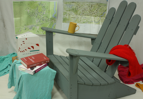
	\begin{overpic}[width=94.40388pt]{imgs/qualitatives/Adirondack_GCNet_disp_h.png} \put(4.0,55.0){$\displaystyle{\color[rgb]{1,1,1}\textbf{30.44\%}}$} \end{overpic}	\begin{overpic}[width=94.40388pt]{imgs/qualitatives/Adirondack_CBMVGCNet_disp_h.png} \put(4.0,55.0){$\displaystyle{\color[rgb]{1,1,1}\textbf{11.10\%}}$} \end{overpic}	\begin{overpic}[width=94.40388pt]{imgs/qualitatives/Adirondack_PSM_h.png} \put(4.0,55.0){$\displaystyle{\color[rgb]{1,1,1}\textbf{31.40\%}}$} \end{overpic}	\begin{overpic}[width=94.40388pt]{imgs/qualitatives/Adirondack_CBMV-PSM.png} \put(4.0,55.0){$\displaystyle{\color[rgb]{1,1,1}\textbf{10.38\%}}$} \end{overpic}
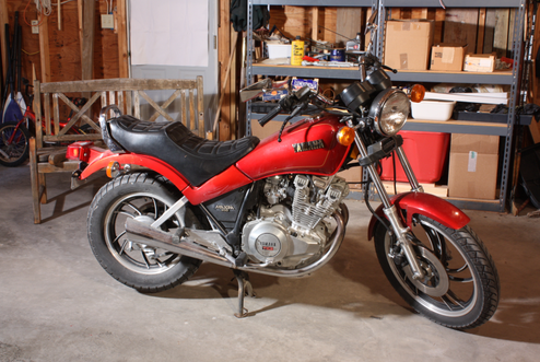
	\begin{overpic}[width=94.40388pt]{imgs/qualitatives/MotorcycleE_GCNet_disp_h.png} \put(4.0,55.0){$\displaystyle{\color[rgb]{1,1,1}\textbf{19.81\%}}$} \end{overpic}	\begin{overpic}[width=94.40388pt]{imgs/qualitatives/MotorcycleE_CBMVGCNet_disp_h.png} \put(4.0,55.0){$\displaystyle{\color[rgb]{1,1,1}\textbf{12.39\%}}$} \end{overpic}	\begin{overpic}[width=94.40388pt]{imgs/qualitatives/MotorcycleE_PSM_h.png} \put(4.0,55.0){$\displaystyle{\color[rgb]{1,1,1}\textbf{46.02\%}}$} \end{overpic}	\begin{overpic}[width=94.40388pt]{imgs/qualitatives/MotorcycleE_CBMV-PSM.png} \put(4.0,55.0){$\displaystyle{\color[rgb]{1,1,1}\textbf{14.57\%}}$} \end{overpic}
(a)	(b)	(c)	(d)	(e)

Figure 4: Qualitative results on Middlebury 2014 [29] for networks trained on sf-all. (a) Reference image, (b) to (e) disparity maps obtained with GCNet [17], MS-GCNet, PSMNet [5] and MS-PSMNet, respectively. Bad2-noc rates are superimposed on the disparities.

4.3 Comparison with State-of-the-art Networks

In addition to a comparative study with respect to their direct 3D counterparts, we compare our MS-Nets with eleven 2D and 3D state-of-the-art networks from the literature. To this aim, we follow the protocol of [35] and compute the accuracy on KT12 and KT15 after training on SceneFlow dataset (sf-all). Table 2 summarizes these comparisons. MS-GCNet proves to be the best architecture at generalization in both domains, outperforming models that makes use of aggressive augmentation strategies (e.g., iResNet) as well as concurrent proposals based on domain-normalization [47]. This confirms that learning disparity estimation in Matching Space enables better generalization in totally unseen environments compared to carrying out the learning process in RGB space. MS-PSMNet is often outperformed on KT12, while it is consistently more effective than eight out of ten baselines on KT15, as already observed in the previous experiments.

4.4 Generalization across Real Domains

In the next set of experiments, reported in Table 3, we investigated the generalization of the networks pre-trained on synthetic data and then specialized on real data from a different domain. Specifically, we pre-trained all networks on sf-all and then continued training for 300 more epochs on KT12, ETH3D or both datasets.

One of the key observations from Table 3 is that GCNet and PSMNet perform well on KT15, when data from KT12 are included in their training, but perform poorly otherwise (see column 1 and 3). MS-Nets have more stable performance even when the real domain used for specialization changes. GCNet and PSMNet perform poorly on MB since all the real domains on which they were trained have dissimilar appearance to it. On the other hand, the MS-Nets achieve higher accuracy on MB, considering that most end-to-end networks fail on this dataset.

4.5 Evaluation on Source Domain Benchmark

It is critical to see our MS-Nets not only show better generalization to unseen domains, but also obtain comparable performance to their counterparts, GCNet and PSMNet, on the test set of the source domains. Following the same protocol as GCNet and PSMNet, our models are firstly trained on synthetic data and fine-tuned on the KITTI 2015 and KITTI 2012 training sets, before being evaluated on the respective test sets. Table 4 and the KITTI leaderboards show the test errors, with virtually no accuracy loss on KITTI 2015 and a moderate drop on KITTI 2012. These results demonstrate that the cost of obtaining a network that generalizes well is small in terms of loss in specialization.

4.6 Qualitative Results

Figure 3 depicts an example from KITTI 2015 following the protocol of Section 4.1. MS-GCNet and MS-PSMNet produce almost smooth disparities on planar surfaces such as roads, whereas PSMNet and GCNet fail at handling the shift from the synthetic domain. For more examples in outdoor environments, we refer readers to the supplementary video sequences comparing GCNet with MS-GCNet and PSMNet with MS-PSMNet on KITTI raw sequence 2011_10_03_drive_0034_sync. Figure 4 shows how MS-style models are much more accurate on Middlebury, better preserving in both cases the overall structure of the scene. For example, MS-PSMNet can recover small details such as the cup on top of the armrest (top row) or the front wheel of the motorcycle (bottom row) which are lost by PSMNet.

5 Conclusions

We have introduced a novel family of 3D convolutional architectures for dense stereo matching, namely MS-Nets. By learning to reason on relationships in matching space without directly being affected by image appearance, our models show superior generalization to unseen domains. The matching space encodes invariant properties that have been proven to be effective in conventional stereo matching. Deep networks such as PSMNet, on the other hand, are purely data-driven and are unable to learn all relevant principles from their training data. Our approach strikes a balance between the empirical modeling and data-driven learning. Conversely to known approaches for tackling the domain shift problem [25, 37, 40, 49], our method can be transferred without the need for retraining or adaptation to new domains, thus presenting an appealing alternative for deployment in real applications.

Our experiments on two state-of-the-art 3D convolutional architectures, GCNet and PSMNet, and their respective MS counterparts, trained on different amounts of synthetic data, confirm that MS-Nets generalize better to different realistic image context, both indoors and outdoors. Additional experiments comparing the generalization performance of MS-Nets with that of ten additional state-of-the-art CNNs for stereo matching show that MS-GCNet is superior in accuracy on unseen data (Section 4.3).

Acknowledgements.    This research has been partially supported by National Science Foundation under Awards IIS-1527294 and IIS-1637761. We gratefully acknowledge the support of NVIDIA Corporation with the donation of the Titan Xp GPU used for this research.

Supplement

In this supplementary document, we present additional qualitative results on domain generalization (i.e., sf-all $\rightarrow$ others), which are omitted in the main paper due to space limits.

Qualitative results from sf-all $\rightarrow$ KT15    In Fig. 5 we provide more qualitative results on KITTI 2015 (KT15) [23] for the networks trained on sf-all [21]. Every two rows correspond to an example from the KT15 training set. Specifically, Fig. 5(a) shows the reference image and ground truth, Fig. 5(b) to (e) show the disparity (top) and error (bottom) maps obtained by baseline GCNet [17], our MS-GCNet, baseline PSMNet [5] and our MS-PSMNet, respectively. Please note the bad3-all rates are superimposed on the error maps.

	\begin{overpic}[width=99.36972pt]{imgs/qualitatives/000002_10_gc_err.png} \put(4.0,22.0){$\displaystyle{\color[rgb]{1,1,1}\textbf{38.57\%}}$} \end{overpic}	\begin{overpic}[width=99.36972pt]{imgs/qualitatives/000002_10_msgc_err.png} \put(4.0,22.0){$\displaystyle{\color[rgb]{1,1,1}\textbf{6.16\%}}$} \end{overpic}	\begin{overpic}[width=99.36972pt]{imgs/qualitatives/000002_10_psm_err.png} \put(4.0,22.0){$\displaystyle{\color[rgb]{1,1,1}\textbf{40.51\%}}$} \end{overpic}	\begin{overpic}[width=99.36972pt]{imgs/qualitatives/000002_10_mspsm_err.png} \put(4.0,22.0){$\displaystyle{\color[rgb]{1,1,1}\textbf{15.93\%}}$} \end{overpic}
	\begin{overpic}[width=99.36972pt]{imgs/qualitatives/000054_10_gc_err.png} \put(4.0,22.0){$\displaystyle{\color[rgb]{1,1,1}\textbf{3.04\%}}$} \end{overpic}	\begin{overpic}[width=99.36972pt]{imgs/qualitatives/000054_10_msgc_err.png} \put(4.0,22.0){$\displaystyle{\color[rgb]{1,1,1}\textbf{1.21\%}}$} \end{overpic}	\begin{overpic}[width=99.36972pt]{imgs/qualitatives/000054_10_psm_err.png} \put(4.0,22.0){$\displaystyle{\color[rgb]{1,1,1}\textbf{8.33\%}}$} \end{overpic}	\begin{overpic}[width=99.36972pt]{imgs/qualitatives/000054_10_mspsm_err.png} \put(4.0,22.0){$\displaystyle{\color[rgb]{1,1,1}\textbf{3.05\%}}$} \end{overpic}
	\begin{overpic}[width=99.36972pt]{imgs/qualitatives/000100_10_gc_err.png} \put(4.0,22.0){$\displaystyle{\color[rgb]{1,1,1}\textbf{23.98\%}}$} \end{overpic}	\begin{overpic}[width=99.36972pt]{imgs/qualitatives/000100_10_msgc_err.png} \put(4.0,22.0){$\displaystyle{\color[rgb]{1,1,1}\textbf{4.21\%}}$} \end{overpic}	\begin{overpic}[width=99.36972pt]{imgs/qualitatives/000100_10_psm_err.png} \put(4.0,22.0){$\displaystyle{\color[rgb]{1,1,1}\textbf{25.46\%}}$} \end{overpic}	\begin{overpic}[width=99.36972pt]{imgs/qualitatives/000100_10_mspsm_err.png} \put(4.0,22.0){$\displaystyle{\color[rgb]{1,1,1}\textbf{5.33\%}}$} \end{overpic}
	\begin{overpic}[width=99.36972pt]{imgs/qualitatives/000104_10_gc_err.png} \put(4.0,22.0){$\displaystyle{\color[rgb]{1,1,1}\textbf{94.16\%}}$} \end{overpic}	\begin{overpic}[width=99.36972pt]{imgs/qualitatives/000104_10_msgc_err.png} \put(4.0,22.0){$\displaystyle{\color[rgb]{1,1,1}\textbf{61.03\%}}$} \end{overpic}	\begin{overpic}[width=99.36972pt]{imgs/qualitatives/000104_10_psm_err.png} \put(4.0,22.0){$\displaystyle{\color[rgb]{1,1,1}\textbf{99.69\%}}$} \end{overpic}	\begin{overpic}[width=99.36972pt]{imgs/qualitatives/000104_10_mspsm_err.png} \put(4.0,22.0){$\displaystyle{\color[rgb]{1,1,1}\textbf{73.08\%}}$} \end{overpic}
	\begin{overpic}[width=99.36972pt]{imgs/qualitatives/000128_10_gc_err.png} \put(4.0,22.0){$\displaystyle{\color[rgb]{1,1,1}\textbf{22.42\%}}$} \end{overpic}	\begin{overpic}[width=99.36972pt]{imgs/qualitatives/000128_10_msgc_err.png} \put(4.0,22.0){$\displaystyle{\color[rgb]{1,1,1}\textbf{1.78\%}}$} \end{overpic}	\begin{overpic}[width=99.36972pt]{imgs/qualitatives/000128_10_psm_err.png} \put(4.0,22.0){$\displaystyle{\color[rgb]{1,1,1}\textbf{24.66\%}}$} \end{overpic}	\begin{overpic}[width=99.36972pt]{imgs/qualitatives/000128_10_mspsm_err.png} \put(4.0,22.0){$\displaystyle{\color[rgb]{1,1,1}\textbf{2.42\%}}$} \end{overpic}
	\begin{overpic}[width=99.36972pt]{imgs/qualitatives/000136_10_gc_err.png} \put(4.0,22.0){$\displaystyle{\color[rgb]{1,1,1}\textbf{24.07\%}}$} \end{overpic}	\begin{overpic}[width=99.36972pt]{imgs/qualitatives/000136_10_msgc_err.png} \put(4.0,22.0){$\displaystyle{\color[rgb]{1,1,1}\textbf{13.12\%}}$} \end{overpic}	\begin{overpic}[width=99.36972pt]{imgs/qualitatives/000136_10_psm_err.png} \put(4.0,22.0){$\displaystyle{\color[rgb]{1,1,1}\textbf{29.43\%}}$} \end{overpic}	\begin{overpic}[width=99.36972pt]{imgs/qualitatives/000136_10_mspsm_err.png} \put(4.0,22.0){$\displaystyle{\color[rgb]{1,1,1}\textbf{13.83\%}}$} \end{overpic}
	\begin{overpic}[width=99.36972pt]{imgs/qualitatives/000150_10_gc_err.png} \put(4.0,22.0){$\displaystyle{\color[rgb]{1,1,1}\textbf{32.67\%}}$} \end{overpic}	\begin{overpic}[width=99.36972pt]{imgs/qualitatives/000150_10_msgc_err.png} \put(4.0,22.0){$\displaystyle{\color[rgb]{1,1,1}\textbf{6.80\%}}$} \end{overpic}	\begin{overpic}[width=99.36972pt]{imgs/qualitatives/000150_10_psm_err.png} \put(4.0,22.0){$\displaystyle{\color[rgb]{1,1,1}\textbf{39.06\%}}$} \end{overpic}	\begin{overpic}[width=99.36972pt]{imgs/qualitatives/000150_10_mspsm_err.png} \put(4.0,22.0){$\displaystyle{\color[rgb]{1,1,1}\textbf{9.49\%}}$} \end{overpic}
	\begin{overpic}[width=99.36972pt]{imgs/qualitatives/000166_10_gc_err.png} \put(4.0,22.0){$\displaystyle{\color[rgb]{1,1,1}\textbf{28.87\%}}$} \end{overpic}	\begin{overpic}[width=99.36972pt]{imgs/qualitatives/000166_10_msgc_err.png} \put(4.0,22.0){$\displaystyle{\color[rgb]{1,1,1}\textbf{2.46\%}}$} \end{overpic}	\begin{overpic}[width=99.36972pt]{imgs/qualitatives/000166_10_psm_err.png} \put(4.0,22.0){$\displaystyle{\color[rgb]{1,1,1}\textbf{28.28\%}}$} \end{overpic}	\begin{overpic}[width=99.36972pt]{imgs/qualitatives/000166_10_mspsm_err.png} \put(4.0,22.0){$\displaystyle{\color[rgb]{1,1,1}\textbf{3.23\%}}$} \end{overpic}
	\begin{overpic}[width=99.36972pt]{imgs/qualitatives/000199_10_gc_err.png} \put(4.0,22.0){$\displaystyle{\color[rgb]{1,1,1}\textbf{26.99\%}}$} \end{overpic}	\begin{overpic}[width=99.36972pt]{imgs/qualitatives/000199_10_msgc_err.png} \put(4.0,22.0){$\displaystyle{\color[rgb]{1,1,1}\textbf{3.64\%}}$} \end{overpic}	\begin{overpic}[width=99.36972pt]{imgs/qualitatives/000199_10_psm_err.png} \put(4.0,22.0){$\displaystyle{\color[rgb]{1,1,1}\textbf{27.80\%}}$} \end{overpic}	\begin{overpic}[width=99.36972pt]{imgs/qualitatives/000199_10_mspsm_err.png} \put(4.0,22.0){$\displaystyle{\color[rgb]{1,1,1}\textbf{3.06\%}}$} \end{overpic}
(a)	(b)	(c)	(d)	(e)

Figure 5: Qualitative results on KITTI 2015 [23] for networks trained on sf-all. Every two rows correspond to one example in KITTI 2015 training set. (a) shows reference image and ground truth, (b) to (e) disparity (top) and error (bottom) maps obtained with GCNet [17], MS-GCNet, PSMNet [5] and MS-PSMNet, respectively. Bad3-all rates are superimposed on the error maps.

Qualitative results from sf-all $\rightarrow$ MB    Fig. 6 shows additional qualitative results on Middlebury 2014 (MB) [29] for the networks trained on sf-all. Each row corresponds to an example from the MB training set. Fig. 6(a) shows the reference image, Fig. 6(b) to (e) are the disparity maps obtained by baseline GCNet [17], our MS-GCNet, baseline PSMNet [5] and our MS-PSMNet, respectively. Bad2-noc rates are superimposed on the disparity maps.

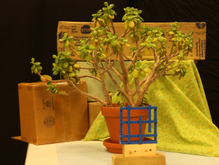
	\begin{overpic}[width=99.36972pt]{imgs/qualitatives/Jadeplant_GC.png} \put(4.0,55.0){$\displaystyle{\color[rgb]{0,0,0}\textbf{48.47\%}}$} \end{overpic}	\begin{overpic}[width=99.36972pt]{imgs/qualitatives/Jadeplant_MS_GC.png} \put(4.0,55.0){$\displaystyle{\color[rgb]{0,0,0}\textbf{20.10\%}}$} \end{overpic}	\begin{overpic}[width=99.36972pt]{imgs/qualitatives/Jadeplant_PSM.png} \put(4.0,55.0){$\displaystyle{\color[rgb]{0,0,0}\textbf{58.63\%}}$} \end{overpic}	\begin{overpic}[width=99.36972pt]{imgs/qualitatives/Jadeplant_MS_PSM.png} \put(4.0,55.0){$\displaystyle{\color[rgb]{0,0,0}\textbf{52.72\%}}$} \end{overpic}
	\begin{overpic}[width=99.36972pt]{imgs/qualitatives/Piano_GCNet_disp.png} \put(4.0,55.0){$\displaystyle{\color[rgb]{0,0,0}\textbf{31.78\%}}$} \end{overpic}	\begin{overpic}[width=99.36972pt]{imgs/qualitatives/Piano_MS_GCNet_disp.png} \put(4.0,55.0){$\displaystyle{\color[rgb]{0,0,0}\textbf{19.91\%}}$} \end{overpic}	\begin{overpic}[width=99.36972pt]{imgs/qualitatives/Piano_PSM.png} \put(4.0,55.0){$\displaystyle{\color[rgb]{0,0,0}\textbf{28.34\%}}$} \end{overpic}	\begin{overpic}[width=99.36972pt]{imgs/qualitatives/Piano_MS_PSM.png} \put(4.0,55.0){$\displaystyle{\color[rgb]{0,0,0}\textbf{23.34\%}}$} \end{overpic}
	\begin{overpic}[width=99.36972pt]{imgs/qualitatives/Pipes_GC.png} \put(10.0,50.0){$\displaystyle{\color[rgb]{0,0,0}\textbf{20.39\%}}$} \end{overpic}	\begin{overpic}[width=99.36972pt]{imgs/qualitatives/Pipes_MS_GC.png} \put(10.0,50.0){$\displaystyle{\color[rgb]{0,0,0}\textbf{10.86\%}}$} \end{overpic}	\begin{overpic}[width=99.36972pt]{imgs/qualitatives/Pipes_PSM.png} \put(10.0,50.0){$\displaystyle{\color[rgb]{0,0,0}\textbf{36.18\%}}$} \end{overpic}	\begin{overpic}[width=99.36972pt]{imgs/qualitatives/Pipes_MS_PSM.png} \put(10.0,50.0){$\displaystyle{\color[rgb]{0,0,0}\textbf{26.42\%}}$} \end{overpic}
	\begin{overpic}[width=99.36972pt]{imgs/qualitatives/PlaytableP_GC.png} \put(4.0,55.0){$\displaystyle{\color[rgb]{0,0,0}\textbf{35.86\%}}$} \end{overpic}	\begin{overpic}[width=99.36972pt]{imgs/qualitatives/PlaytableP_MS_GC.png} \put(4.0,55.0){$\displaystyle{\color[rgb]{0,0,0}\textbf{19.0\%}}$} \end{overpic}	\begin{overpic}[width=99.36972pt]{imgs/qualitatives/PlaytableP_PSM.png} \put(4.0,55.0){$\displaystyle{\color[rgb]{0,0,0}\textbf{32.56\%}}$} \end{overpic}	\begin{overpic}[width=99.36972pt]{imgs/qualitatives/PlaytableP_MS_PSM.png} \put(4.0,55.0){$\displaystyle{\color[rgb]{0,0,0}\textbf{43.69\%}}$} \end{overpic}
	\begin{overpic}[width=99.36972pt]{imgs/qualitatives/Recycle_GC.png} \put(4.0,55.0){$\displaystyle{\color[rgb]{0,0,0}\textbf{25.08\%}}$} \end{overpic}	\begin{overpic}[width=99.36972pt]{imgs/qualitatives/Recycle_MS_GC.png} \put(4.0,55.0){$\displaystyle{\color[rgb]{0,0,0}\textbf{13.51\%}}$} \end{overpic}	\begin{overpic}[width=99.36972pt]{imgs/qualitatives/Recycle_PSM.png} \put(4.0,55.0){$\displaystyle{\color[rgb]{0,0,0}\textbf{25.52\%}}$} \end{overpic}	\begin{overpic}[width=99.36972pt]{imgs/qualitatives/Recycle_MS_PSM.png} \put(4.0,55.0){$\displaystyle{\color[rgb]{0,0,0}\textbf{13.84\%}}$} \end{overpic}
	\begin{overpic}[width=99.36972pt]{imgs/qualitatives/Teddy_GC.png} \put(10.0,70.0){$\displaystyle{\color[rgb]{0,0,0}\textbf{20.62\%}}$} \end{overpic}	\begin{overpic}[width=99.36972pt]{imgs/qualitatives/Teddy_MS_GC.png} \put(10.0,70.0){$\displaystyle{\color[rgb]{0,0,0}\textbf{5.07\%}}$} \end{overpic}	\begin{overpic}[width=99.36972pt]{imgs/qualitatives/Teddy_PSM.png} \put(10.0,70.0){$\displaystyle{\color[rgb]{0,0,0}\textbf{26.49\%}}$} \end{overpic}	\begin{overpic}[width=99.36972pt]{imgs/qualitatives/Teddy_MS_PSM.png} \put(10.0,70.0){$\displaystyle{\color[rgb]{0,0,0}\textbf{15.39\%}}$} \end{overpic}
(a)	(b)	(c)	(d)	(e)

Figure 6: Qualitative results on Middlebury 2014 [29] for networks trained on sf-all. Column (a) shows reference image, (b) to (e) disparity maps obtained with GCNet [17], MS-GCNet, PSMNet [5] and MS-PSMNet, respectively. Bad2-noc rates are superimposed on the disparity maps.

Qualitative results from sf-all $\rightarrow$ KT Raw    We show more qualitative results on KITTI (KT) raw sequence 2011_10_03_drive_0034_sync, for MS-GCNet (Fig. 7) and MS-PSMNet (Fig. 8) trained on sf-all. Specifically, Fig. 7(a) is the input left frame, and Fig. 7(b) and (c) are the disparity maps estimated by baseline GCNet [17] and our MS-GCNet, respectively. Fig 8 provides the results for baseline PSMNet [5] and our MS-PSMNet. Please note there is no ground truth for KT raw sequences, so the error rates cannot be calculated. Still, comparing the disparity maps in (b) and (c), ours tend to predict more reliable and smooth disparities rather than the noisy and bumpy ones by the baselines. For more examples, please see our MS-GCNet video (https://youtu.be/Qr6WGsPX5P8) and MS-PSMNet video (https://youtu.be/t9WPc3pxzc4). Each frame of the videos shows the input left image (top), the disparity map estimated by the baseline (middle), and the disparity map by our MS counterpart (bottom).

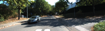
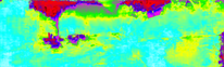
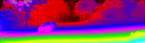
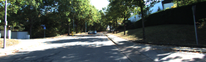
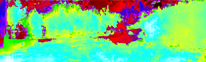
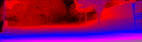
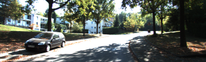
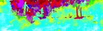
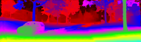
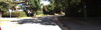
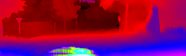
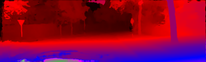
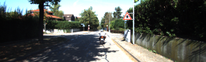
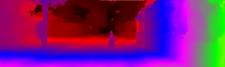
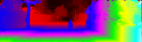
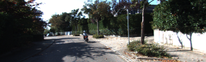
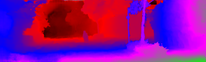
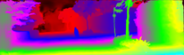
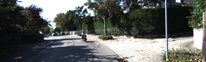
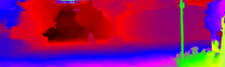
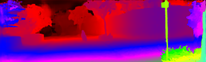
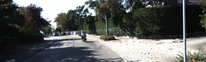
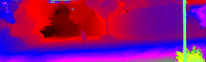
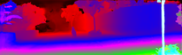
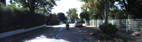
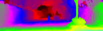
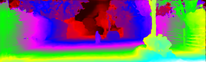
(a)	(b)	(c)

Figure 7: Qualitative results on KITTI raw sequence 2011_10_03_drive_0034_sync, for networks trained on sf-all. (a) Left input frame. (b) Disparity map estimated by GCNet [17]. (c) Disparity map estimated by our MS-GCNet. Both networks are trained on the same synthetic data sf-all.

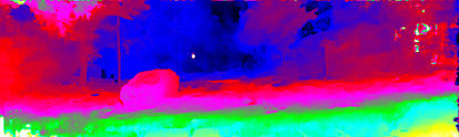
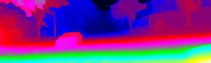
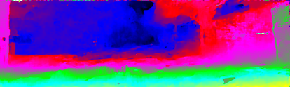
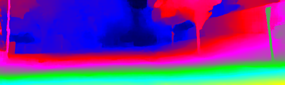
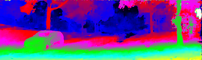
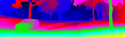
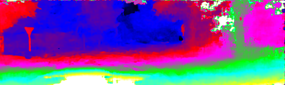
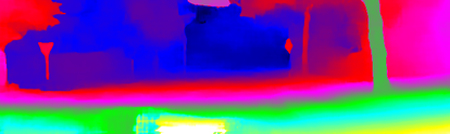
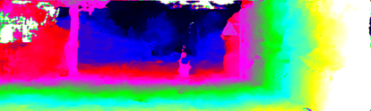
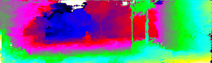
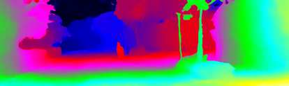
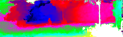
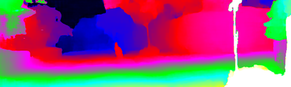
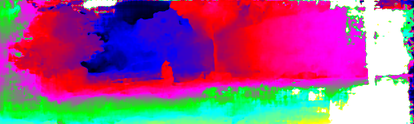
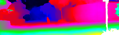
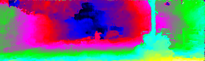
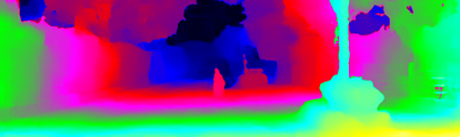
(a)	(b)	(c)

Figure 8: Qualitative results on KITTI raw sequence 2011_10_03_drive_0034_sync, for networks trained on sf-all. (a) Left input frame. (b) Disparity map estimated by PSMNet [5]. (c) Disparity map estimated by our MS-PSMNet. Both networks are trained on the same synthetic data sf-all.

References

- [1] K. Batsos, C. Cai, and P. Mordohai. CBMV: A coalesced bidirectional matching volume for disparity estimation. In CVPR, pages 2060–2069, 2018.
- [2] K. Batsos and P. Mordohai. RecResNet: A recurrent residual cnn architecture for disparity map enhancement. In International Conference on 3D Vision (3DV), pages 238–247, 2018.
- [3] V. Casser, S. Pirk, R. Mahjourian, and A. Angelova. Unsupervised learning of depth and ego-motion: A structured approach. In AAAI Conference on Artificial Intelligence, 2019.
- [4] R. Chabra, J. Straub, C. Sweeney, R. Newcombe, and H. Fuchs. Stereodrnet: Dilated residual stereonet. In CVPR, June 2019.
- [5] J.-R. Chang and Y.-S. Chen. Pyramid stereo matching network. In CVPR, pages 5410–5418, 2018.
- [6] Q. Chen and V. Koltun. Photographic image synthesis with cascaded refinement networks. In ICCV, pages 1511–1520, 2017.
- [7] Z. Chen, X. Sun, L. Wang, Y. Yu, and C. Huang. A deep visual correspondence embedding model for stereo matching costs. In ICCV, pages 972–980, 2015.
- [8] A. Geiger, P. Lenz, and R. Urtasun. Are we ready for autonomous driving? The KITTI vision benchmark suite. In CVPR, 2012.
- [9] S. Gidaris and N. Komodakis. Detect, replace, refine: Deep structured prediction for pixel wise labeling. In CVPR, pages 5248–5257, 2017.
- [10] X. Guo, H. Li, S. Yi, J. Ren, and X. Wang. Learning monocular depth by distilling cross-domain stereo networks. In Proceedings of the European Conference on Computer Vision (ECCV), pages 484–500, 2018.
- [11] X. Guo, K. Yang, W. Yang, X. Wang, and H. Li. Group-wise correlation stereo network. In CVPR, 2019.
- [12] K. He, X. Zhang, S. Ren, and J. Sun. Spatial pyramid pooling in deep convolutional networks for visual recognition. In ECCV, 2014.
- [13] H. Hirschmüller. Stereo processing by semiglobal matching and mutual information. PAMI, 30(2):328–341, 2008.
- [14] J. Hoffman, E. Tzeng, T. Park, J.-Y. Zhu, P. Isola, K. Saenko, A. Efros, and T. Darrell. Cycada: Cycle-consistent adversarial domain adaptation. In ICML, 2018.
- [15] X. Hu and P. Mordohai. A quantitative evaluation of confidence measures for stereo vision. PAMI, 34(11):2121–2133, 2012.
- [16] J. Janai, F. Güney, A. Behl, and A. Geiger. Computer vision for autonomous vehicles: Problems, datasets and state-of-the-art. arXiv preprint arXiv:1704.05519, 2017.
- [17] A. Kendall, H. Martirosyan, S. Dasgupta, P. Henry, R. Kennedy, A. Bachrach, and A. Bry. End-to-end learning of geometry and context for deep stereo regression. In ICCV, pages 66–75, 2017.
- [18] M. Liang, X. Guo, H. Li, X. Wang, and Y. Song. Unsupervised cross-spectral stereo matching by learning to synthesize. In Proceedings of the AAAI Conference on Artificial Intelligence, volume 33, pages 8706–8713, 2019.
- [19] Z. Liang, Y. Feng, Y. Guo, H. Liu, W. Chen, L. Qiao, L. Zhou, and J. Zhang. Learning for disparity estimation through feature constancy. In CVPR, pages 2811–2820, 2018.
- [20] W. Luo, A. G. Schwing, and R. Urtasun. Efficient deep learning for stereo matching. In CVPR, pages 5695–5703, 2016.
- [21] N. Mayer, E. Ilg, P. Hausser, P. Fischer, D. Cremers, A. Dosovitskiy, and T. Brox. A large dataset to train convolutional networks for disparity, optical flow, and scene flow estimation. In CVPR, pages 4040–4048, 2016.
- [22] X. Mei, X. Sun, M. Zhou, S. Jiao, H. Wang, and X. Zhang. On building an accurate stereo matching system on graphics hardware. In ICCV Workshops, pages 467–474, 2011.
- [23] M. Menze and A. Geiger. Object scene flow for autonomous vehicles. In CVPR, pages 3061–3070, 2015.
- [24] J. Pang, W. Sun, J. S. Ren, C. Yang, and Q. Yan. Cascade residual learning: A two-stage convolutional neural network for stereo matching. In Proceedings of the IEEE International Conference on Computer Vision Workshops, pages 887–895, 2017.
- [25] J. Pang, W. Sun, C. Yang, J. Ren, R. Xiao, J. Zeng, and L. Lin. Zoom and learn: Generalizing deep stereo matching to novel domains. In CVPR, pages 2070–2079, 2018.
- [26] M.-G. Park and K.-J. Yoon. Leveraging stereo matching with learning-based confidence measures. In CVPR, pages 101–109, 2015.
- [27] M. Poggi and S. Mattoccia. Learning a general-purpose confidence measure based on o (1) features and a smarter aggregation strategy for semi global matching. In International Conference on 3D Vision (3DV), pages 509–518, 2016.
- [28] M. Poggi, F. Tosi, and S. Mattoccia. Quantitative evaluation of confidence measures in a machine learning world. In ICCV, pages 5228–5237, 2017.
- [29] D. Scharstein, H. Hirschmüller, Y. Kitajima, G. Krathwohl, N. Nešić, X. Wang, and P. Westling. High-resolution stereo datasets with subpixel-accurate ground truth. In German Conference on Pattern Recognition, pages 31–42, 2014.
- [30] D. Scharstein and R. Szeliski. A taxonomy and evaluation of dense two-frame stereo correspondence algorithms. IJCV, 47(1-3):7–42, 2002.
- [31] J. L. Schönberger, S. N. Sinha, and M. Pollefeys. Learning to fuse proposals from multiple scanline optimizations in semi-global matching. In ECCV, pages 739–755, 2018.
- [32] T. Schöps, J. L. Schonberger, S. Galliani, T. Sattler, K. Schindler, M. Pollefeys, and A. Geiger. A multi-view stereo benchmark with high-resolution images and multi-camera videos. In CVPR, pages 3260–3269, 2017.
- [33] A. Seki and M. Pollefeys. Sgm-nets: Semi-global matching with neural networks. In CVPR, pages 231–240, 2017.
- [34] A. Shaked and L. Wolf. Improved stereo matching with constant highway networks and reflective confidence learning. In CVPR, pages 4641–4650, 2017.
- [35] X. Song, X. Zhao, L. Fang, and H. Hu. EdgeStereo: An effective multi-task learning network for stereo matching and edge detection. IJCV, 2020.
- [36] T. Taniai, Y. Matsushita, Y. Sato, and T. Naemura. Continuous 3D label stereo matching using local expansion moves. PAMI, 40(11):2725–2739, 2018.
- [37] A. Tonioni, M. Poggi, S. Mattoccia, and L. Di Stefano. Unsupervised adaptation for deep stereo. In ICCV, pages 1605–1613, 2017.
- [38] A. Tonioni, M. Poggi, S. Mattoccia, and L. D. Stefano. Unsupervised domain adaptation for depth prediction from images. IEEE Transactions on Pattern Analysis and Machine Intelligence, 42(10):2396–2409, 2020.
- [39] A. Tonioni, O. Rahnama, T. Joy, L. D. Stefano, T. Ajanthan, and P. H. Torr. Learning to adapt for stereo. In CVPR, June 2019.
- [40] A. Tonioni, F. Tosi, M. Poggi, S. Mattoccia, and L. Di Stefano. Real-time self-adaptive deep stereo. In CVPR, June 2019.
- [41] C.-W. Xie, H.-Y. Zhou, and J. Wu. Vortex pooling: Improving context representation in semantic segmentation. arXiv preprint arXiv:1804.06242, 2018.
- [42] G. Yang, H. Zhao, J. Shi, Z. Deng, and J. Jia. SegStereo: Exploiting semantic information for disparity estimation. In ECCV, pages 636–651, 2018.
- [43] Z. Yin, T. Darrell, and F. Yu. Hierarchical discrete distribution decomposition for match density estimation. In CVPR, June 2019.
- [44] L. Yu, Y. Wang, Y. Wu, and Y. Jia. Deep stereo matching with explicit cost aggregation sub-architecture. In AAAI Conference on Artificial Intelligence, 2018.
- [45] J. Žbontar and Y. LeCun. Stereo matching by training a convolutional neural network to compare image patches. Journal of Machine Learning Research, 17(1-32):2, 2016.
- [46] F. Zhang, V. Prisacariu, R. Yang, and P. H. Torr. Ga-net: Guided aggregation net for end-to-end stereo matching. In CVPR, 2019.
- [47] F. Zhang, X. Qi, R. Yang, V. Prisacariu, B. Wah, and P. Torr. Domain-invariant stereo matching networks. In ECCV, 2020.
- [48] Y. Zhong, Y. Dai, and H. Li. Self-supervised learning for stereo matching with self-improving ability. arXiv preprint arXiv:1709.00930, 2017.
- [49] Y. Zhong, H. Li, and Y. Dai. Open-world stereo video matching with deep RNN. In ECCV, pages 101–116, 2018.