Causal Multi-Level Fairness

Abstract.

Algorithmic systems are known to impact marginalized groups severely, and more so, if all sources of bias are not considered. While work in algorithmic fairness to-date has primarily focused on addressing discrimination due to individually linked attributes, social science research elucidates how some properties we link to individuals can be conceptualized as having causes at macro (e.g. structural) levels, and it may be important to be fair to attributes at multiple levels. For example, instead of simply considering race as a causal, protected attribute of an individual, the cause may be distilled as perceived racial discrimination an individual experiences, which in turn can be affected by neighborhood-level factors. This multi-level conceptualization is relevant to questions of fairness, as it may not only be important to take into account if the individual belonged to another demographic group, but also if the individual received advantaged treatment at the macro-level. In this paper, we formalize the problem of multi-level fairness using tools from causal inference in a manner that allows one to assess and account for effects of sensitive attributes at multiple levels. We show importance of the problem by illustrating residual unfairness if macro-level sensitive attributes are not accounted for, or included without accounting for their multi-level nature. Further, in the context of a real-world task of predicting income based on macro and individual-level attributes, we demonstrate an approach for mitigating unfairness, a result of multi-level sensitive attributes.

1. Introduction

There has been much recent interest in designing algorithms that make fair predictions (Kroll et al., 2016; Diakopoulos et al., 2017; Barocas et al., 2017). Definitions of algorithmic fairness have been summarized in detail elsewhere (Verma and Rubin, 2018; Mishler et al., 2021); broadly approaches to algorithmic fairness in machine learning can be divided into two kinds: group fairness, which ensures some form of statistical parity for members of different protected groups (Dwork et al., 2012; Mishler et al., 2021) and individual notions of fairness which aim to ensure that people who are ‘similar’ with respect to the classification task receive similar outcomes (Binns, 2020; Joseph et al., 2016; Biega et al., 2018). Historically sensitive variables such as age, gender, race have been thought of as attributes that can lead to unfairness or discrimination. Recently, the causal framework (Pearl et al., 2000) has also been used to conceptualize fairness. Kusner et al. (2017) introduced a causal definition of fairness, counterfactual fairness, which states that a decision is fair toward an individual if it coincides with the one that would have been taken in a counterfactual world in which the sensitive attribute of the individual had been different. This approach assumes prior knowledge about how data is generated and how variables affect each other, represented by a causal diagram and considers that all paths from the sensitive attribute to the outcome are unfair. Counterfactual fairness, thus, postulates that the entire effect of the sensitive attribute on the decision, along all causal paths from the sensitive attribute to the outcome is unfair. This approach is restrictive when only certain causal paths are unfair. For example, the effect of gender on income levels can be considered unfair but the effect through education attainment level is fair (Chiappa, 2019). Path-specific counterfactual fairness has then been conceptualized, which attempts to correct the effect of the sensitive attribute on the outcomes only along unfair causal pathways instead of entirely removing the effect of the sensitive attribute (Chiappa, 2019). It should be noted that throughout this work, determination of fair and unfair paths requires domain expertise and possibly discussions between policymakers, lawyers, and computer scientists.

Leveraging domain knowledge from sociology highlights that notwithstanding these clarifications of path-specific fairness, algorithmic fairness efforts in general have been limited to sensitive attributes at only the individual-level, missing important assertions regarding how social aspects can be influenced and created more by societal structures and cultural assumptions than by individual and psychological factors (Kincheloe and McLaren, 2011). Critical Theory is an approach in sociology which motivates the consideration of macro-structural attributes, often simply called macro-properties or ‘structural attributes’. These structural attributes correspond to overall organizations of society that extend beyond the immediate milieu of individual attributes yet have an impact on an individual, such as social groups, organizations, institutions, nation-states, and their respective properties and relations (Furze and Savy, 2014; Little et al., 2016). Accounting for a multi-level conceptualization in algorithmic fairness is consistent with recent literature which have discussed similar concerns with the conceptualization of race as a fixed, individual-level attribute (VanderWeele and Robinson, 2014; Hanna et al., 2020; Zuberi, 2000; Boyd et al., 2020). Analytically framing race as an individual-level attribute ignores systemic racism and other factors which are the mechanisms by which race has consequences (Boyd et al., 2020). Instead, accounting for the macro-level phenomena associated with race, which a multi-level perspective promotes (e.g. structural racism, childhood experiences that shape the perception of race) will augment the impact of algorithmic fairness work (Hanna et al., 2020). Several different terms have been used as synonyms for macro-structural attributes, including “group-level” variables in multi-level analysis, “ecological variables”, “macro-level variables”, “contextual variables”, “group variables”, and “population variables”, and we refer the reader to a full elaboration on macro-property variables in previous work by Diez-Roux (1998). In this paper, we refer to all information measured beyond an individual-level as macro-properties and macro-level attributes.

Without accounting for macro-properties, assessment of how “fair” an algorithm is may inadvertently be unfair by not accounting for important variance in attributes that are at the structural level. Indeed, today’s growing availability of data that captures such effects means that leveraging the right data can be used to account for and address unexplained variance when using individual-level attributes as proxies for structural attributes. This can help work towards equity versus in-sample fairness (e.g. an algorithm fair with respect to perceived race will still be unfair to structural differences that perceived race may be a proxy for, such as neighborhood socio-economics, and including the structural factors can help to mitigate unfairness within the perceived race category) (Mhasawade et al., 2020). Accounting for structural factors can also clearly identify populations that input data is not representing. Indeed, many macro-properties can be considered as sensitive attributes. For example, neighborhood socioeconomic status which is a measure of the inequality in distribution of macro-level resources of education, work, and economic resources(Ross and Mirowsky, 2008). It has been shown that patients who reside in low socioeconomic neighborhoods can have significantly higher risk for readmission following hospitalization for sepsis in comparison to patients residing in higher socioeconomic neighborhoods even if all individual-level risk factors are the same, indicating that low SES is an independent factor of relevance to the outcome (Galiatsatos et al., 2020). Thus, accounting for relevant macro-level properties while making decisions, say, about post-hospitalization care, is critical to ensure that disadvantaged patients, comprehensively accounting for all relevant sources of unfairness, receive appropriate care.

(a) Proxy ($I^{N}$) for sensitive attributes ($A_{I}$)

(b) Multiple sensitive attributes $A_{I}^{G},A_{I}^{R}$

(c)

Figure 1. Causal graphs to describe and distinguish different general sensitive attribute settings. Green arrows denote discriminatory causal paths and dashed green-black arrows from any node $R$ to $S$ denote discrimination only due to the portion of the effect from a green arrow into $R$ and not from $R$ itself (fair paths defined via a priori knowledge), red nodes represent sensitive attributes. a) Individual-level variable $I^{N}$ (e.g. name) acts as a proxy for the individual sensitive attribute $A_{I}$ (e.g. perceived race) and affects outcome $Y$ (e.g. health outcomes). $I^{B}$ (e.g. a biological factor) is not a proxy but also affects the outcome. b) Multiple sensitive attributes at the individual level, $A_{I}^{G}$ (e.g. gender) and $A_{I}^{R}$ (e.g. perceived race) affect individual variables, $I$, and health outcome, $Y$. c) Example of cycles in the causal graph, where individual level attribute $I$, individual income, causes macro-level sensitive attribute, mean neighborhood income, $A_{P}$, which in turn affects education resources in the neighborhood, $P$, with $Y$ being the outcome. Since $I\in pa_{A_{P}}$, this violates the necessary conditions for obtaining a fair predictor with multi-level causal fairness.

Towards this goal, we propose a novel definition of fairness called causal multi-level fairness, which is defined as a decision being fair towards an individual if it coincides with the one in the counterfactual world where, contrary to what is observed, the individual receives advantaged treatment at both the macro and individual levels, described by macro and individual-level sensitive attributes, respectively. This work builds upon previous work on path-specific counterfactual fairness, limited to individual-level sensitive attributes, to account for both macro and individual-level discrimination. Multi-level sensitive attributes are a specific case of multiple sensitive attributes, in which we specifically consider a sensitive attribute at a macro level that influences one at an individual level. This is an important and broad class of settings; such multi-level interactions are also considered in multi-level modelling in statistics (Gelman, 2006). Moreover, this work addresses a different problem than the setting of proxy variables, in which the aim is to eliminate influence of the proxy on outcome prediction (Kilbertus et al., 2017). Indeed, for variables such as race, detailed analyses from epidemiology have articulated how concepts such as racial inequality can be decomposed into the portion that would be eliminated by equalizing adult socioeconomic status across racial groups, and a portion of the inequality that would remain even if adult socioeconomic status across racial groups were equalized (i.e. racism). Thus, if we simply ascribe the race variable to the individual (as is sometimes done as a proxy), we will miss the population-level factors that affect it and any particular outcome (VanderWeele and Robinson, 2014).

Explicitly accounting for multi-level factors enables us to decompose concepts such as racial inequality and approach questions such as: what would the outcome be if there was a different treatment on a population-level attribute such as neighborhood socioeconomic status? This is an important step in auditing not just the sources of bias that can lead to discriminatory outcomes but also in identifying and assessing the level of impact of different causal pathways that contribute to unfairness. Given that in some subject areas, the most effective interventions are at the macro level (e.g. in health the largest opportunity for decreasing incidence due to several diseases lie with the social determinants of health such as availability of resources versus individual-level attributes (Mhasawade et al., 2020)), it is critical to have a framework to assess these multiple sources of unfairness. Moreover, by including macro-level factors and their influence on individual ones, we engage themes of inequality and power by specifying attributes outside of an individual’s control. In sum, our work is one step towards integrating perspectives that articulate the multi-dimensionality of sensitive attributes (for example race, and other social constructs) into algorithmic approaches. We do this by bringing focus to social processes which often affect individual attributes, and developing a framework to account for multiple casual pathways of unfairness amongst them. Our specific contributions are:

• We formalize multi-level causal systems, which include potentially fair and unfair path effects at both macro and individual-level sensitive variables. Such a framework enables the algorithmicist to conceptualize systems that include the systemic factors that shape outcomes.

• Using the above framework, we demonstrate that residual fairness can result if macro-level attributes are not accounted for.

• We provide necessary conditions for achieving multi-level fairness and demonstrate an approach for mitigating multi-level unfairness while retaining model performance.

2. Related Work

Causal Fairness. Several statistical fairness criteria have been introduced over the last decade, to ensure models are fair with respect to group fairness metrics or individual fairness metrics. However, further discussions have highlighted that several of the fairness metrics cannot be concurrently satisfied on the same data (Kleinberg et al., 2016; Chouldechova, 2017; Friedler et al., 2016; Berk et al., 2018; Kasy and Abebe, 2021; McCradden et al., 2020). In light of this, causal approaches to fairness have been recently developed to provide a more intuitive reasoning corresponding to domain specifics of the applications (Kilbertus et al., 2017; Kusner et al., 2017, 2019; Bonchi et al., 2017; Qureshi et al., 2016; Russell et al., 2017; Kusner et al., 2018; Zhang and Bareinboim, 2018a, b; Nabi and Shpitser, 2018; Nabi et al., 2019b; Chiappa, 2019). Most of these approaches advocate for fairness by addressing an unfair causal effect of the sensitive attribute on the decision. Kusner et al. (2017) have introduced an individual-level causal definition of fairness, known as counterfactual fairness. The intuition is that the decision is fair if it coincides with the one that would have been taken in a counterfactual world in which the individual would be identified by a different sensitive attribute. For example, a hiring decision is counterfactually fair if the individual identified by the gender male would have also been offered the job had the individual identified as female. In sum, these efforts develop concepts of fairness with respect to individual level sensitive attributes, while here we develop fairness accounting for multi-level sensitive attributes, comprising of both individual and macro-level sensitive attributes. Inspired from research in social sciences (VanderWeele and Robinson, 2014; Hanna et al., 2020; Binns, 2020), the work here extends the idea to multi-level sensitive attributes. In our considered setting, a decision is fair not only if the individual identified with a different individual-level sensitive attribute but also if the individual received advantaged treatment at the macro-level, attributed as the macro-level sensitive attribute.

Identification of Causal Effects. While majority of the work in causal inference is on identification and estimation of the total causal effect (Tian and Pearl, 2002; Avin et al., 2005; Pearl, 2001; Pearl et al., 2000; Peters et al., 2017), studies have also looked at identifying the causal effect along certain causal pathways (Shpitser, 2013; Pearl, 2013). The most common approach for identifying the causal effect along different causal pathways is decomposing the total causal effect along direct and indirect pathways (Pearl, 2013, 2012; Shpitser, 2013). We leverage the approach developed by Shpitser (2013) on how causal effects of multiple variables along a single causal pathway can be identified. While we assume no unmeasured confounding for the analysis in this work, research in causal estimation in the presence of unmeasured confounding, (Miao et al., 2018; Wang and Blei, 2019) can be used to extend our current contribution.

Path-specific causal fairness. Approaches in causal fairness such as path-specific counterfactual fairness (Nabi and Shpitser, 2018; Chiappa, 2019; Nabi et al., 2019b), proxy discrimination, and unresolved discrimination (Kilbertus et al., 2017; Wu et al., 2019) have aimed to understand the effect of sensitive attributes (i.e. variables that correspond to gender, race, disability, or other protected attributes of individuals) on outcomes directly as well as indirectly to identify the causal pathways (represented using a causal diagram) that result into discriminatory predictions of outcomes based on the sensitive attribute. Generally such approaches focus on sensitive attributes at the individual-level and require an understanding of the discriminatory causal pathways for mitigating causal discrimination along the specified pathways. Our approach builds on the work of Chiappa (2019) for mitigating unfairness by removing path-specific effects for fair predictions, doing so while accounting for both individual and macro-level unfairness.

Intersectional fairness. There is recent focus on identifying the impact of multiple sensitive attributes (intersectionality) on model predictions. There are several works that have been developed for this setting (Foulds et al., 2020; Yang et al., 2020a; Morina et al., 2019), however, these approaches do not take into account the different causal interactions between sensitive attributes themselves which can be important in identifying bias due to intersectionality. In particular, this includes intersectional attributes at the individual and macro level, such as race and socioeconomic status (Coley et al., 2015; Kuo et al., 2020).

3. Background

We begin by introducing the tools needed to outline multi-level fairness, namely, (1) causal models, (2) their graphical definition, (3) causal effects, and (4) counterfactual fairness.

Causal Models: Following Pearl et al. (2000) we define a causal model as a triple of sets $\left(\textbf{U},\textbf{V},F\right)$ such that:

• U are a set of latent variables, which are not caused by any of the observed variables in V.

• $F$ is set of functions for each $V_{i}\in\textbf{V}$, such that
  $V_{i}=f_{i}\left(\mathit{pa}_{i},U_{pa_{i}}\right)$, $pa_{i}\subseteq\textbf{V}\setminus V_{i}$ and $U_{pa_{i}}\subseteq\textbf{U}$. Such equations relating $V_{i}$ to $pa_{i}$ and $U_{pa_{i}}$ are known as structural equations (De Arcangelis, 1993). When $f_{i}$ is strictly linear, this is known as a linear structural equation model, which is represented as $V_{i}=\sum_{j=1}^{|pa_{i}|}\alpha_{j}\cdot pa_{i}[j]+U_{pa_{i}}$, where $\alpha$ is the mixing coefficient and $pa_{i}[j]$ denotes the $j$th parent of variable $V_{i}$.

Here, “$pa_{i}$” refers to the causal parents of $V_{i}$, i.e. the variables that affect the specific value $V_{i}$ obtains. The joint distribution over all the $n$ variables, $\text{Pr}\left(V_{1},V_{2},\cdots,V_{n}\right)$ is given by the product of the conditional distribution of each variable, $V_{i}$, given it’s causal parents $pa_{i}$ as follows:

(1) $$\text{Pr}\left(\textbf{V}\right)=\prod_{i}\text{Pr}\left(V_{i}|\mathit{pa}_{i}\right).$$

Graphical definition of causal models: While structural equations define the relations between variables we can graphically represent the causal relationships between random variables using Graphical Causal Models (GCMs) (Chiappa, 2019). The nodes in a GCM represent the random variables of interest, $V$, and the edges represent the causal and statistical relationships between them. Here, we restrict our analysis to Directed Acyclic Graphs (DAGs) where there are no cycles, i.e., a node cannot have an edge both originating from and terminating at itself. Furthermore, a node $Y$ is known as a child of another node $X$ if there is an edge between the two that originates at $X$ and terminates on $Y$. Here, $X$ is called a direct cause of $Y$. If $Y$ is a descendant of $X$, with some other variable $Z$ along the path from $X$ to $Y$, $X\rightarrow\cdots\rightarrow Z\rightarrow\cdots Y$, then $Z$ is known as a mediator variable and $X$ remains as a potential cause of $Y$. For example, in Figure 1(b), $A_{I}^{G},A_{I}^{R},I,Y$ are the random variables of interest. $A_{I}^{G},A_{I}^{R}$ are direct causes of $I$ and $Y$ while $I$ is a direct cause of $Y$. Here, $I$ is known as a mediating variable for both $A_{I}^{G}$ and $A_{I}^{R}$.

Causal effects: The causal effect of $X$ on $Y$ is the information propagated by $X$ towards $Y$ via the causal directed paths, $X\rightarrow\cdots\rightarrow Y$. This is equal to the conditional distribution of $Y$ given $X$ if there are no bidirected paths between $X$ and $Y$. A bidirected path between $X$ and $Y$, $X\leftarrow\cdots\rightarrow Y$ represents confounding; that is some causal variable known as a confounder, which may be unobserved, affecting both $X$ and $Y$. If confounders are present then the causal effect can be estimated by intervening upon $X$. This means that we externally set the value of $X$ to the desired value $x$ and remove any edges that terminate at $X$, since manually setting $X$ to $x$ would inhibit any causation by $pa_{x}$. After intervening the causal effect of $X$ on $Y$ is given by $\text{Pr}^{*}\left(Y|X=x\right)=\sum_{Z}\text{Pr}\left(Y|X=x,Z\right)\text{Pr}\left(Z\right)$, where $Z=\mathbf{V}\setminus\{X,Y\}$. The intervention $X=x$ results into a potential outcome, $Y_{X=x}$ (also represented as $Y_{x}$), where the distribution of the potential outcome variable is defined as $\text{Pr}\left(Y_{x}\right)=\text{Pr}^{*}\left(Y|X=x\right)$.

Counterfactual fairness: Counterfactual fairness is a causal notion of fairness that restricts the decisions of the algorithm to be invariant to the value assigned to the sensitive variable. Assuming $A$ to be the sensitive attribute obtaining only two values, $a$ and $a^{\prime}$, $X$ as the remaining variables, and $Y$ as the outcome of interest, counterfactual fairness is defined as follows:

Definition 3.0.

Predictor $\hat{Y}$ is counterfactually fair if under any context $X$ and $A=a$,

(2) $$\small\text{Pr}(\hat{Y}_{A\rightarrow a}(U)=y|X,A=a)=\text{Pr}(\hat{Y}_{A\rightarrow a^{\prime}}(U)=y|X,A=a)$$

With this background, we next discuss the problem setup.

4. Problem Setup

Let us denote all the variables associated with the system being modelled as $\textbf{V}:=\{A_{I},A_{P},\textbf{I},\textbf{P},Y\}$, where $A_{I}$ and $A_{P}$ are the sensitive attributes at the individual-level and the macro-level respectively, I is a non empty set of individual level variables, P is a non empty set of macro-level variables, and $Y$ is an outcome of interest. We assume access to a causal graph, $\mathcal{G}$, consisting of V which accurately represents the data-generating process. Our goal is to obtain a classifier, $\hat{Y}_{\text{fair}}$, which is fair with respect to both $A_{P}$ and $A_{I}$. While previous approaches in algorithmic fairness have only considered $A_{I}$ as a sensitive attribute, we present a novel approach to also counter any discrimination resulting from $A_{P}$. While macro-level attributes, $\mathbf{P}$ and $A_{P}$, may seem like regular nodes in the causal graph, the difference is that based on them being macro-properties, their effects on the outcome may be mediated via the individual level attributes, $\mathbf{I}$ and $A_{I}$, making it nontrivial to mitigate unfairness due to these macro-properties. We highlight that this paper presents, to our knowledge, the first approach for incorporating unfairness due to macro-properties into algorithmic fairness. In order to further help guide the reader regarding differences in macro and individual-level variables, we clarify the types of macro-level attributes which are considered in our setting. Per the extant literature (Diez-Roux, 1998), macro-level attributes can be categorized into two types:

• Category 1: non-aggregate group properties like nationality, existence of certain types of regulations, population density, degree of income inequality in a community, political regime, legal status of women which do not include individual properties in their computation

• Category 2: aggregate properties such as neighborhood income and median household income, which include individual properties (here individual income) in their computation

Thus, individual variables influence aggregate macro-properties (Category 2) but not non-aggregate macro-properties (Category 1). This categorization of macro-properties helps us to identify the necessary conditions for obtaining a fair classifier with respect to both individual and macro-level sensitive attributes. In parallel, a main assumption in causal fairness and causal inference settings is that we have access to a causal graph and that the graph does not include any bidirected edges or cycles, (Chiappa, 2019; Nabi and Shpitser, 2018; Kusner et al., 2017) which are assumptions we maintain for the causal multi-level fairness setting. This assumption also clarifies that we should limit our consideration of macro-level attributes to Category 1 and not consider aggregate information like mean neighborhood income as macro-level sensitive variables since individual-level information has a causal influence on mean neighborhood income, i.e. $I\rightarrow A_{P}$. Certainly, an increase in the individual income increases mean neighborhood income, which can result in feedback loops in the causal graph which are disallowed. Figure 1(c) represents such a case involving cycles which the current framework does not support. Further, we assume that the structural equation model representing the functional form underlying the causal graph is linear in nature, i.e. a node is a linear combination of its causal parents. Future work should extend the analysis to non-linear relationships and non-parametric forms. We also assume that we are aware about the fair and unfair causal paths for the multi-level sensitive attributes, again consistent with previous work (Chiappa, 2019). Next, we present an example to realize the importance of macro-level sensitive attributes.

4.1. An Illustrative Example

In prior sections we have motivated the need to consider macro-level attributes. We now describe multi-level sensitive attributes and provide an illustrative example of why considering macro-level sensitive attributes in algorithmic fairness efforts can be important. Consider neighborhood socioeconomic status (SES) as $A_{P}$. Neighborhood SES can be a cause of population-level factors such as resources available. Neighborhood SES can also affect individual-level attributes, $A_{I}$ such as perception of race (which is protected), by shaping the cultural and social experiences of an individual (Dailey et al., 2010) as well as non-protected attributes, $I$ (e.g. body-mass index, given that neighborhood SES can shape the types of resources available and norms (Mathur et al., 2013)). Furthermore, research has described how macro attributes such as neighborhood SES can affect health behaviors like smoking directly as well as through individual factors such as perceived racial discrimination. Thus, given that this macro-attribute shapes the resources and circumstances of an individual ($A_{I}$ can be influenced by $A_{P}$), it could be desirable for algorithms which are being used to decide fair allocation of health services or resources to predicted smokers, to account for this macro-property. Not being fair to this property lacks consideration for variance within the individual attributes that it influences. In other words, accounting for only individual-level attributes such as perceived racial discrimination can still lead to unfairness without considering that people within the same individual-level category could have different resources or opportunities available to them.

A general framework for macro/individual attribute relationships and possible unfair paths in presented in Figure 2. In illustrating the relationship between $A_{P}$ and $A_{I}$ (green arrow) we make distinction between the multi-level fairness setting and literature on intersectionality in fairness, which has considered multiple sensitive attributes that are independent of each other (Figure 1(b)) (Foulds et al., 2020; Morina et al., 2019; Yang et al., 2020a, b). While this assumption of independence may hold for individual-level sensitive attributes like age and gender, it fails when we consider sensitive attributes at both the individual and macro level. It is important to understand the relationship between individual and macro-level attributes in order to delineate the path-specific effects that may lead to biased predictions of $Y$.

Next, we describe how these interactions can lead to unfairness, by introducing multi-level path-specific fairness accounting for both individual and macro-level sensitive attributes.

5. Multi-level path-specific fairness

We begin the discussion about multi-level path-specific fairness by first introducing path-specific effects, discussing the necessary conditions to identify the effects with multiple sensitive attributes, and finally describe an approach to obtain fair predictions with multi-level path specific effects.

Figure 2. Multi-level sensitive attributes $A_{I},A_{P}$. Macro-level variables, $A_{P}$ (e.g. neighborhood SES), $P$ (e.g. other zipcode level factors), and individual-level ones, $A_{I}$ (e.g. perceived racial discrimination), $I$, affect the outcome $Y$ (e.g. a health behavior).

5.1. Path-specific effects

While counterfactual fairness assumes that the entire effect of the sensitive variables on the outcomes is problematic and constructs the predictor with only the non-descendants of the sensitive attribute (Kusner et al., 2017), it is a fairly restrictive scenario especially when the sensitive attributes can affect the outcome along both fair and unfair pathways as shown in Figure 2. Thus, disregarding the effect only along unfair paths can help in preserving the fair individual information regarding sensitive attributes (Chiappa, 2019). Indeed, domain experts and policymakers can guide these decisions about identifying fair and unfair pathways. We are interested only in correcting the effect of the sensitive attribute on the outcome along the unfair paths. For this we turn to path-specific effects, which isolate the causal effect of a treatment on an outcome only along a certain causal pathway (Pearl, 2001). In order to obtain the causal effect only along a certain pathway, the idea that path-specific effects can be formulated as nested counterfactuals is leveraged (Shpitser, 2013). This is done by considering that along the causal path of interest, say, $A_{I}\rightarrow I\rightarrow Y$, the variable, $A_{I}$, propagates the observed value, for example, $a_{i}$ in Figure 2, and along other pathways, $A_{I}\rightarrow Y$, the counterfactual value, $a_{i}^{\prime}$ is propagated, assuming that $A_{I}=\{a_{i},a_{i}^{\prime}\}$. In this case, the effect of any mediator between $A_{I}$ and $Y$ is evaluated according to the corresponding value of $A_{I}$ propagated along the specific causal path, the mediator $I$ obtains the value $I(a_{i})$. Here, the primary object of interest is the potential outcome variable, $Y(a_{i})$, which represents the outcome if, possibly contrary to fact, $A_{I}$ were externally set to value $a_{i}$. Given the values of $a_{i},a_{i}^{\prime}$, comparison of $Y(a_{i}^{\prime})$ and $Y(a_{i})$ in expectation: $\mathbb{E}[Y(a_{i})]-\mathbb{E}[Y(a_{i}^{\prime})]$ would allow us to quantify the path-specific causal effect, PSE, of $A_{I}$ on $Y$.

Using this concept of path-specific effect, we next state path-specific counterfactual fairness, defined by Chiappa (2019).

Definition 5.0.

Path-specific counterfactual fairness is defined as a decision being fair towards an individual if it coincides with the one that would have been made in a counterfactual world in which the sensitive attribute along the unfair pathways (denoted by $\pi$) was set to the counterfactual value.

(3) $$\small\text{Pr}(\hat{Y}_{A\rightarrow a_{\pi}}(U)=y|X,A=a)=\text{Pr}(\hat{Y}_{A\rightarrow a^{\prime}_{\pi}}(U)=y|X,A=a)$$

Chiappa (2019) further propose that in order to obtain a fair decision, the path-specific effect of the sensitive attribute along the discriminatory causal paths is removed from the model predictions, i.e. $\hat{Y}_{\text{fair}}=\hat{Y}-\text{PSE}$. However, a key limitation of the approach presented by Chiappa (2019) is that only the path-specific counterfactual fairness with respect to the sensitive attributes at the individual level is considered. The presence of sensitive attributes at the macro-level that affect properties at the individual level makes it non-trivial to estimate the path-specific effect consisting of both macro and individual-level sensitive attributes. Following, we describe the identifiability conditions for obtaining path-specific counterfactual fairness with respect to multi-level sensitive attributes by estimating multi-level path-specific effects.

Identification of multi-level path-specific effects.

Proposition 1.

In the absence of any unmeasured confounding between $A_{P}$ and $A_{I}$ and $\{A_{I},\textbf{I}\}\not\in pa_{A_{P}}$, the multi-level path-specific effects of both $A_{P}$ and $A_{I}$ on $Y$ are identifiable.

Proposition 1 follows from the possible structural interactions between $A_{P}$ and $A_{I}$, where $A_{P}$ is a non-aggregate macro-property not involving any individual-level computation. Next, we discuss the interaction between $A_{P}$ and $A_{I}$, where the macro-level sensitive attribute is a causal parent of the individual-level sensitive attribute, $A_{P}\in\{pa_{A_{I}}\}$.

Figure 2 presents such an exemplar case of multi-level interactions where macro-level sensitive attributes can cause individual level variables, with the data generating process as described in Figure 3(a). $A_{P}$ and $A_{I}$ are binary variables where we assume $a_{p}^{\prime}$ and $a_{i}^{\prime}$ to represent the baseline values denoting advantaged treatments. The rest of the variables $P,I$ and $Y$ are continuous and follow a linear relationship between the parents and the specific variables. $\epsilon_{p},\epsilon_{a_{i}},\epsilon_{i},\epsilon_{y}$ are unobserved zero-mean Gaussian terms. For this specific model we obtain the multi-level path-specific effects consisting of both $A_{P}$ and $A_{I}$. The population level sensitive attribute, $A_{P}$ affects $Y$ via multiple paths along 1) $A_{P}\rightarrow P\rightarrow Y$, 2) $A_{P}\rightarrow I\rightarrow Y$, 3) $A_{P}\rightarrow A_{I}\rightarrow Y$, and 4) $A_{P}\rightarrow A_{I}\rightarrow I\rightarrow Y$; the individual level sensitive attribute $A_{I}$ affects $Y$ along two causal paths, 1) $A_{I}\rightarrow I\rightarrow Y$, and 2) $A_{I}\rightarrow Y$. With prior assumption that $A_{I}\rightarrow Y$ and $P\rightarrow Y$ are not discriminatory causal paths, we evaluate the path-specific effect along $\cdots\rightarrow I\rightarrow Y$, where $\cdots\rightarrow I$ repesents all paths into $I$ . Overall the path-specific effect can be calculated as follows:

(4) $$\text{PSE}_{A_{P}\leftarrow a_{p},A_{I}\leftarrow a_{i}}^{\cdots\rightarrow I\rightarrow Y}=\mathbb{E}\left[Y\left(a_{i}^{\prime},P\left(a_{p}^{\prime}\right),I\left(a_{i},a_{p}\right)\right)\right].$$

The path-specific effect along $\cdots\rightarrow I\rightarrow Y$ is computed by comparison of the counterfactual variable $Y\left(a_{i}^{\prime},P\left(a_{p}^{\prime}\right),I\left(a_{i},a_{p}\right)\right)$, where $a_{p},a_{i}$ are set to the baseline value of 1 in the counterfactual and 0 in the original. The counterfactual distribution can be estimated as follows:

(5) $$Y\left(a_{i}^{\prime},P\left(a_{p}^{\prime}\right),I\left(a_{i},a_{p}\right)\right)$$

$$=\int_{P,I}\text{Pr}\left(Y|a_{i}^{\prime},I,P\right)\text{Pr}\left(I|a_{i},a_{p}\right)\text{Pr}\left(P|a_{p}^{\prime}\right).$$

We obtain the mean of this distribution as follows:

(6) $$\mathbb{E}[Y|I,P,a_{i}^{\prime}]$$

$$=\theta^{y}_{\phantom{i}}+\theta^{y}_{i}\theta^{i}+\theta^{y}_{p}\theta^{p}+\theta^{y}_{a_{i}}a_{i}^{\prime}+\theta^{y}_{i}\theta^{i}_{a_{i}}a_{i}+\theta^{y}_{i}\theta^{i}_{a_{p}}a_{p}+\theta^{y}_{p}\theta^{p}_{a_{p}}a_{p}^{\prime}.$$

$\text{PSE}_{A_{P}\leftarrow a_{p},A_{I}\leftarrow a_{i}}^{\cdots\rightarrow I\rightarrow Y}$ is then obtained by comparing the observed and counterfactual value of the mean of the counterfactual distribution,

(7) $$\small\begin{split}\mathbb{E}[Y|a_{p},a_{i}]-\mathbb{E}[Y|a_{p}^{\prime},a_{i}^{\prime}]&=\theta^{y}_{a_{i}}\left(a_{i}^{\prime}-a_{i}^{\prime}\right)+\theta^{y}_{i}\theta^{i}_{a_{i}}\left(a_{i}-a_{i}^{\prime}\right)\\ &+\theta^{y}_{i}\theta^{i}_{a_{p}}\left(a_{p}-a_{p}^{\prime}\right)+\theta^{y}_{p}\theta^{p}_{a_{p}}\left(a_{p}^{\prime}-a_{p}^{\prime}\right)\\ &=\theta^{y}_{i}\theta^{i}_{a_{i}}\left(a_{i}-a_{i}^{\prime}\right)+\theta^{y}_{i}\theta^{i}_{a_{p}}\left(a_{p}-a_{p}^{\prime}\right).\end{split}$$

Substituting $a_{i}=1,a_{p}=1,a_{i}^{\prime}=0,a_{p}^{\prime}=0$ in Equation 7 we obtain the path-specific effect as a function of the parameters $\theta$:

(8) $$\text{PSE}^{\cdots\rightarrow I\rightarrow Y}_{A_{P}\leftarrow a_{p},A_{I}\leftarrow a_{i}}=\theta^{y}_{i}\theta^{i}_{a_{i}}+\theta^{y}_{i}\theta^{i}_{a_{p}}.$$

By the same approach, path-specific effects for individual and macro-level sensitive attributes as well as the multi-level path specific effects for all the causal paths in Figure 2, are also evaluated. Estimating the multi-level path-specific effects helps in constructing a fair predictor which is described in the following section.

Algorithm 1 Causal Multi-level Fairness

  Input: Causal Graph $\mathcal{G}$ consisting of nodes $V$, data $\mathcal{D}$ over $V$, discriminatory causal pathways $\pi$, $\beta$.

  Output: Fair predictor $\hat{Y}_{\text{fair}}$, model parameters $\theta$

  for $V_{i}\in\textbf{V}$ do

     Estimate $\hat{\theta}^{V_{i}}\leftarrow\operatorname*{arg\,min}_{\theta}\sum_{k\in\mathcal{D}}l\left(V_{i}^{(k)},f_{i}\left(pa_{i}^{(k)}\right)\right)$

  end for

  Calculate path-specific effects, PSE along $\pi$ using $\theta^{\textbf{V}}$

  return $\hat{Y}_{\text{fair}}=\mathbb{E}\left[f_{Y}\left(\theta^{Y}\right)\right]-\beta*\text{PSE}_{\pi}$

$$\begin{split}&A_{P}\sim\text{Bernoulli}\left(p=0.5\right),\\ &P=\theta^{p}_{\phantom{p}}+\theta^{p}_{a_{p}}A_{P}+\epsilon_{p},\\ &\gamma=\theta^{a_{i}}+\theta^{a_{i}}_{a_{p}}A_{P}+\theta^{a_{i}}_{p}P+\epsilon_{a_{i}},\\ &A_{I}=\text{Bernoulli}(\sigma(\gamma)),\\ &I=\theta^{i}_{\phantom{p}}+\theta^{i}_{a_{p}}A_{P}+\theta^{i}_{a_{i}}A_{I}+\epsilon_{i},\\ &Y=\theta^{y}_{\phantom{p}}+\theta^{y}_{p}P+\theta^{y}_{i}I+\theta^{y}_{a_{i}}A_{I}+\epsilon_{y}\\ &\theta^{p},\theta^{a_{i}},\theta^{i},\theta^{y}=\left(0.2,0.2,0.2,0.2\right)\\ &\theta^{p}_{a_{p}},\theta^{a_{i}}_{a_{p}},\theta^{a_{i}}_{p},\theta^{i}_{a_{p}},\theta^{i}_{a_{i}}\sim U\left(0.2,0.7\right)\\ &\theta^{y}_{p},\theta^{y}_{i},\theta^{y}_{a_{i}}\sim U\left(0.3,0.95\right)\\ &\epsilon_{p},\epsilon_{a_{i}},\epsilon_{i},\epsilon_{y}\sim\mathcal{N}\left(0,1\right)\\ &\sigma=1/\left(1+\text{exp}\left(-x\right)\right)\end{split}$$

(a)

$A_{P}$	$\theta^{y}_{p}\theta^{p}_{a_{p}}$
$A_{P},A_{I}$	$\theta^{y}_{p}\theta^{p}_{a_{p}}+\theta^{y}_{i}\theta^{i}_{a_{i}}$

(b)

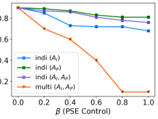
(c)

Figure 3. Experimental details regarding multi-level example (Figure 2), a) Data generating process, b) Resulting causal graph if $A_{P}$ is considered as an individual-level sensitive attribute instead of macro-level sensitive attribute as presented in Figure 2, $A_{P}\not\in pa_{A_{I}}$, resulting path-specific effects with $A_{P}$ as individual-level sensitive attribute, and c) Path-specific unfairness controlling for discriminatory effects of just $A_{I}$ (blue), $A_{P}$ considered as an individual-level sensitive attribute instead of macro-level sensitive attribute (green), both $A_{I},A_{P}$ considered as individual-level sensitive attributes (purple), and $A_{I},A_{P}$ considered as multi-level sensitive attributes (orange), over 10 runs.

5.2. Fair predictions with multi-level path-specific effects.

Fair outcomes can be estimated by removing the unfair path-specific effect from the prediction (essentially making a correction on all the descendants of the sensitive attributes), $\hat{Y}$ by simply subtracting it, i.e. $\hat{Y}_{\text{fair}}=\hat{Y}-\text{PSE}$. As done in Chiappa (2019), removing such unfair information at test time ensures that the resulting decision coincides with the one that would have been taken in a counterfactual world in which the sensitive attribute along the unfair pathways were set to the baseline. We leverage this same idea for multi-level causal fairness by generating fair predictions, $\hat{y}_{\text{fair}}$, by controlling for the path-specific effects of multi-level sensitive attributes. For example, consider the PSE resulting from intervening upon both $A_{P}$ and $A_{I}$ via the path $\dots\rightarrow I\rightarrow Y$, $\text{PSE}_{A_{P}\leftarrow a_{p},A_{I}\leftarrow a_{i}}^{\cdots\rightarrow I\rightarrow Y}=\theta^{y}_{i}\left(\theta^{i}_{a_{i}}+\theta^{i}_{a_{p}}\right)$, we can control for the discrimination at test time as follows:

(9) $$\hat{y}^{n}_{\text{fair}}=\theta^{y}_{\phantom{a}}+\theta^{y}_{p}p^{n}+\theta^{y}_{i}i^{n}+\theta^{y}_{a}a_{i}^{n}-\beta\left(\theta^{y}_{i}\left(\theta^{i}_{a_{i}}+\theta^{i}_{a_{p}}\right)\right)$$

where $\beta$ accounts for the control over the path-specific effect. For our analysis $\beta$ ranges from 0 to 1, where $0$ denotes that we do not account for any path-specific effect while 1 denotes that we remove the entire path-specific effect. Intermediate values allow for only partial removal of the path-specific effect. We study the effect of the control over different path-specific effects on the performance metric of the classifier. The steps are outlined in Algorithm 1. We highlight that an accurate causal graph and a linear functional form are key assumptions of this approach.

6. Experiments

Our experiments in this section serve to empirically assess and demonstrate residual unfairness when correcting for path-specific effects of multiple sensitive attributes. We consider a synthetic setting demonstrated in Figure 2 and real-world setting for income prediction presented in Figure 4(a); in both cases the structural causal model is known a priori as well as the unfair pathways. In each case, we first learn the parameters of the model ($\Theta$) from the observed data based on the known underlying causal graph, $\mathcal{G}$ as illustrated in Algorithm 1. We then draw observed and counterfactual samples from the distribution $\theta$ by sampling from the path-specific counterfactual distribution, referred to as counterfactual distribution. We estimate fair predictors for both the observed and counterfactual data using Algorithm 1. In case of no resultant unfairness, distributions of the outcome estimate for both observed and counterfactual data should coincide. Density plots that do not coincide signifies residual unfairness.

6.1. Synthetic setting

Here we generate data according to the structural equation model presented in Figure 3(a) with linear relationships with the exception that we consider $Y$ to be binary, using a sigmoid function . This represents the data-generating process in accordance with the multi-level setting presented in Figure 2. The simulation parameters, $\theta$, are non-negative to ensure a positive path-specific effect, i.e. an unfair effect. Furthermore, the parameters are standardized between 0 and 1 to allow for computational efficiency. The range of the parameters in the uniform distribution is simulated to ensure a realistic setting where the counterfactual distribution is diverse, and the differences between the original and counterfactual distribution is significant to evaluate multi-level fairness. If there are little differences in the original and the counterfactual distribution, path-specific effects become negligible resulting in no significant unfairness issues. In total, 10 simulations with $N=2000$ samples in each are performed. We train a linear regression model for $I,P$, and a logistic regression model for $A_{I},Y$ to learn the parameters ($\theta$). We then calculate three path-specific effects as follows: 1) $\text{PSE}_{A_{P},A_{I}}$ accounting for the effect of both $A_{P}$ and $A_{I}$, 2) $\text{PSE}_{A_{I}}$ accounting for the effect of only $A_{I}$, and 3) $\text{PSE}_{A_{P}}$ accounting for the effect of only $A_{P}$. Details about this calculation are presented in Equation 7.

We observe that controlling for the multi-level path-specific effects of both $A_{P}$ and $A_{I}$ leads to little drop in the model performance (accuracy). We also assess the counterfactual fairness of the resulting model after removing the unfair multi-level path-specific effects. This is done by training a classifier for obtaining fair predictors, $\hat{y}_{a_{i},a_{p}}$, on the actual and counterfactual data respectively, where the counterfactual data is obtained by altering the values of the sensitive variables, $A_{P}$ and $A_{I}$. This is done by first learning the parameters, $\theta$ from the original data and then altering the values of the sensitive attributes, $A_{P}$ and $A_{I}$ and obtaining the values of $P,I$ and $Y$ from these counterfactual values of $A_{P},A_{I}$ and $\theta$. We assess the counterfactual fairness of the resulting models while accounting for unfairness due to both $A_{P},A_{I}$ and either $A_{I}$ or $A_{P}$, in Figure 3(c). The Y axis shows the average difference between observed and counterfactual predictions, $|\hat{Y}_{a}-\hat{Y}_{a^{\prime}}|$ where $a$ is the observed value of the sensitive attribute and $a^{\prime}$ is the corresponding counterfactual value. This difference is analyzed for varying control of the path-specific effect (PSE), $\beta$ along the X-axis. In order to assess the advantage of considering the multi-level nature of the data, we compare with the model presented in Figure 3(b), where we treat the macro-level sensitive attribute, $A_{P}$ as another individual-level sensitive attribute, $A_{I}$, i.e. $A_{P}\not\in pa_{A_{I}}$. The blue line represents the difference while accounting only for the individual-level path specific effect $A_{I}$ while the orange line represents the multi-level path-specific effect of both $A_{P}$ and $A_{I}$. Similarly, the green line represents the setting presented in Figure 3(b), where $A_{P}$, is treated as an individual-level sensitive attribute (multi-level nature of its action removed), and purple line represents the case where both $A_{I}$ and $A_{P}$ are treated as individual-level sensitive attributes. For counterfactually fair models we expect the difference to be close to zero since controlling for the path-specific effects cancels out the counterfactual change. We observe that this happens only while accounting for the multi-level path-specific effects. Thus, accounting for individual-level path-specific effects solely (blue, green, and purple lines) does not result in counterfactually fair predictions as can be seen from the high difference (0.7- 0.9). Moreover, correcting for the unfair multi-level path-specific effects of both $A_{P}$ and $A_{I}$ results in counterfactually fair predictions with a slight drop in accuracy from 94.5% to 91.5%.

6.2. UCI Adult Dataset

(a)

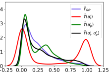
(b)

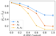
(c)

Figure 4. a) Causal graph for the UCI Adult dataset (Chiappa, 2019), $A$ and $M$ represent the individual-level protected attributes, sex and marital status, respectively, $C$ is age and nationality, $L$ is the level of education, $R$ corresponds to working class, occupation, and hours per week, $Y$ is the income class, unfair paths are represented in green b) Density of $\hat{Y}$, c) path-specific unfairness, $|\hat{Y}_{a}-\hat{Y}_{a^{\prime}}|$ controlling for the effects of just $A_{I}$ (blue), $A_{P}$ (orange) and both $A_{I},A_{P}$ (yellow).

We demonstrate real-world evaluation of the proposed approach on the Adult dataset from the UCI repository (Lichman et al., 2013). The UCI Adult dataset is amenable for demonstration of our method, given that it was used in Chiappa (2019) to assess path-specific counterfactual fairness, and because there are variables oriented in a manner that create a potential multi-level scenario. We consider this well-studied setting (Chiappa, 2019; Nabi and Shpitser, 2018) wherein the goal is to predict whether an individual’s income is above or below $50,000. The data consist of age, working class, education level, marital status, occupation, relationship, race, gender, capital gain and loss, working hours, and nationality variables for 48842 individuals. The causal graph is represented in Figure 4(a). Consistent with Chiappa (2019) and Nabi and Shpitser (2018), we do not include race or capital gain and loss variables. Here, $A$ represents the individual-level protected attribute sex, $C$ is nationality, $M$ is marital status, $L$ is the level of education, $R$ corresponds to working class, occupation, and hours per week, $Y$ is the income class. We make an observation that nationality, $C$, could be considered as a non-aggregate macro-level sensitive attribute. This is because it may affect social influences and/or resources available at the macro-level. For example, nationality affects both education levels and martial status of individuals. Moreover, we also note that marital status, $M$, can also be considered as an individual-level sensitive attribute, as we may not want to discriminate individuals based on their marital status (Joslin, 2015; Reimers, 1985). Thus, $C$, a macro-level sensitive attribute affects $M$, an individual-level sensitive attribute and the relationship between $C$ and other variables in the graph mimics that of a multi-level scenario. Moreover, it may be reasonable to consider a setting in which it is desirable to predict income, while also being fair to nationality, in order to understand the effect that nationality may have. We highlight that macro-properties such as nationality are included in datasets like UCI adult, however, correcting for any unfairness due to macro-level sensitive attributes has not been considered in previous fairness studies. We also emphasize that there may be other datasets that better express the need for macro and individual-level sensitive attributes, however we consider this dataset/setting in order to be consistent with previous work in causal fairness which has used the same dataset, though have only analyzed unfairness due to an individual-level sensitive attribute (Chiappa, 2019). Paths in Figure 4(a) are thus defined based on mapping the figure from Chiappa (2019) to the multi-level framework in Figure 1(b) with $C$ as the macro-level sensitive attribute and $A$, $M$ as the individual-level sensitive attributes.

To first evaluate the path-specific effect of a single individual-level sensitive attribute as done in prior work (Chiappa, 2019), we evaluate the effect of only $A$ (the individual level sensitive attribute considered in Chiappa (2019)) along $A\rightarrow Y$ and $A\rightarrow M\rightarrow\cdots\rightarrow Y$ to be 3.716. We obtain a fair prediction as follows:

$$\hat{y}_{\text{fair}}=\text{Bernoulli}\left(\sigma\left(\theta^{y}+\theta^{y}_{c}C+\theta^{y}_{m}\left(M-\theta^{m}_{a}\right)+\theta^{y}_{l}\left(L-\theta^{l}_{m}\theta^{m}_{a}\right)\right)\right)$$

by removing the path specific effect of $A$ along a priori known discriminatory paths. The fair accuracy is 78.87%, consistent with Chiappa (2019).

We next evaluate the path-specific effect of both the macro ($C$) and individual-level sensitive attributes ($A,M$). In the counterfactual world, the individual receives advantaged macro and individual level treatment. Since, $C$ is mostly represented by the value 39, and $A$ is represented by 2 levels 0 and 1, worst to best, we consider the baseline values to be $c=39$ and $a=1$. We compute the path-specific effect of $C$ on $Y$ via $C\rightarrow M\rightarrow\cdots\rightarrow Y$, $C\rightarrow L\rightarrow\cdots\rightarrow Y$, $A\rightarrow M\rightarrow\cdots\rightarrow Y$, and $A\rightarrow Y$ in the baseline scenario to be 10.65. As we do not completely remove the effect of $C$; only along certain paths as described above, we still retain important information about nationality, $C$, an informative feature. After correcting for the unfair effect of $C$, $A$, and $M$, the accuracy is 77.92% ($\beta=1$), in comparison with an accuracy of 78.87% from removing the unfair effect of $A$ alone. Thus, there is not significant drop in the model performance after correcting for the unfair effects of both $A,M$ and $C$.

Next, we study the residual unfairness in a series of counterfactual settings which account for unfairness at individual, macro-level sensitive attributes and their combination. Results are presented in Figure 4(b). If density of two plots coincide, then they are counterfactually fair, i.e. there is no difference in prediction based on unfair pathways. The purple plot represents the fair model, $\hat{Y}_{\text{fair}}$, trained on the original data that corrects for the multi-level path-specific effects of $\{A,M,C\}$. In the process of learning the fair predictions, we learn the parameters for the model represented in Figure 4(a) as illustrated in Algorithm 1 and then generate counterfactual samples from the observed distribution. We next assess fairness of models that account for varying fair/unfair pathways and variable types. First, we generate individual-level counterfactual data by only altering the individual-level sensitive attributes $A$ and $M$ along the unfair pathways, and train a model on the individual-level counterfactual data, we call this $\hat{Y}\left(a_{i}^{\prime}\right)$. The red curve represents the density plot of $\hat{Y}\left(a_{i}^{\prime}\right)$ after controlling for the individual-level path-specific effect at $\beta=1$. Similarly, we generate macro-level counterfactual data by only altering the macro-level sensitive attribute, $C$, along the unfair paths, $C\rightarrow M\rightarrow\cdots,C\rightarrow L\rightarrow\cdots$, and train a model on this macro-level counterfactual data, which is represented by $\hat{Y}(a_{p}^{\prime})$ (green curve). At last, we generate individual and macro-level counterfactual data, by altering $A,M$ and $C$ along all unfair paths, represented by green in Figure 4(a). In this case, the predictor, $\hat{Y}(a_{i}^{\prime},a_{p}^{\prime})$, is represented by the black curve, As can be seen from the general overlap of the purple and black curves, controlling for path-specific effects of both individual and macro-level sensitive attributes generates counterfactually fair models, while only controlling for the individual or macro variables doesn’t provide the same density estimate as a fair model. Similarly, the residual unfairness is presented in Figure 4(c), and controlling for the multi-level path-specific effects (yellow curve) results in a counterfactual fair model as the difference, $|\hat{Y}_{a}-\hat{Y}_{a^{\prime}}|$ approaches zero. Thus, correcting the multi-level path specific effect does not marginally drop the model performance, while ensuring that predictions are fair with respect to individual and macro-level attributes.

7. Conclusion

Our work extends algorithmic fairness to account for the multi-level and socially-constructed nature of forces that shape unfairness. In doing so, we first articulate a new definition of fairness, multi-level fairness. Multi-level fairness articulates a decision being fair towards the individual if it coincides with the one in the counterfactual world where, contrary to what is observed, the individual identifies with the advantaged sensitive attribute at the individual-level and also receives advantaged treatment at the macro-level described by the macro-level sensitive attribute. A framework like this can be used to assess unfairness at each level, and identify the places for intervention that would reduce unfairness best (e.g. via macro-level policies versus individual attributes). As we show here, leveraging datasets that represent more than individual attributes can improve fairness, as often individual level attributes have variance with respect to macro-properties, or are proxies for macro-properties which may be the critical sources of unfairness (Mhasawade et al., 2020). This is becoming possible given the large number of open data sets representing macro-attributes that are available, relevant to health, economics, and many other settings. Through our experiments, we illustrate the importance of accounting for macro-level sensitive attributes by exhibiting residual unfairness if they are not accounted for. Importantly, we show this residual unfairness persists even in cases when the same information and variables are considered, but without accounting for the multi-level nature of their interaction.

Finally, we demonstrate a method for achieving fair outcomes by removing unfair path-specific effects with respect to both individual and macro-level sensitive attributes. While a clear understanding of the macro-level sensitive attributes is essential for multi-level fairness, approaches to learning the latent representation of the macro-level sensitive attributes in their absence from individual-level factors could be important future work. As an initial framework, we consider path-specific effects for linear models here; we also endeavor to extend this to fewer assumptions on the functional form in the future.

References

- (1)
- Adams et al. (2007) Maurianne Ed Adams, Lee Anne Ed Bell, and Pat Ed Griffin. 2007. Teaching for diversity and social justice. Routledge/Taylor & Francis Group.
- Avin et al. (2005) C Avin, I Shpitser, and J Pearl. 2005. Identifiability of Path Specific Effects, In Proceedings of International Joint Conference on Artificial Intelligence. Edinburgh, Scotland 357 (2005), 363.
- Barocas et al. (2017) Solon Barocas, Kate Crawford, Aaron Shapiro, and Hanna Wallach. 2017. The Problem with Bias: From Allocative to Representational Harms in Machine Learning’. Special Interest Group for Computing, Information and Society (SIGCIS) 2 (2017).
- Berk et al. (2018) Richard Berk, Hoda Heidari, Shahin Jabbari, Michael Kearns, and Aaron Roth. 2018. Fairness in criminal justice risk assessments: The state of the art. Sociological Methods & Research (2018), 0049124118782533.
- Biega et al. (2018) Asia J Biega, Krishna P Gummadi, and Gerhard Weikum. 2018. Equity of attention: Amortizing individual fairness in rankings. In The 41st international acm sigir conference on research & development in information retrieval. 405–414.
- Binns (2020) Reuben Binns. 2020. On the apparent conflict between individual and group fairness. In Proceedings of the 2020 Conference on Fairness, Accountability, and Transparency. 514–524.
- Bonchi et al. (2017) Francesco Bonchi, Sara Hajian, Bud Mishra, and Daniele Ramazzotti. 2017. Exposing the probabilistic causal structure of discrimination. International Journal of Data Science and Analytics 3, 1 (2017), 1–21.
- Boyd et al. (2020) Rhea W Boyd, Edwin G Lindo, Lachelle D Weeks, and Monica R McLemore. 2020. On racism: a new standard for publishing on racial health inequities. Health Affairs Blog 10 (2020).
- Chiappa (2019) Silvia Chiappa. 2019. Path-specific counterfactual fairness. In Proceedings of the AAAI Conference on Artificial Intelligence, Vol. 33. 7801–7808.
- Chouldechova (2017) Alexandra Chouldechova. 2017. Fair prediction with disparate impact: A study of bias in recidivism prediction instruments. Big data 5, 2 (2017), 153–163.
- Coley et al. (2015) Sheryl L Coley, Tracy R Nichols, Kelly L Rulison, Robert E Aronson, Shelly L Brown-Jeffy, and Sharon D Morrison. 2015. Race, socioeconomic status, and age: exploring intersections in preterm birth disparities among teen mothers. International journal of population research 2015 (2015).
- Dailey et al. (2010) Amy B Dailey, Stanislav V Kasl, Theodore R Holford, Tene T Lewis, and Beth A Jones. 2010. Neighborhood-and individual-level socioeconomic variation in perceptions of racial discrimination. Ethnicity & health 15, 2 (2010), 145–163.
- De Arcangelis (1993) Giuseppe De Arcangelis. 1993. Structural Equations with Latent Variables.
- Diakopoulos et al. (2017) Nicholas Diakopoulos, Sorelle Friedler, Marcelo Arenas, Solon Barocas, Michael Hay, Bill Howe, Hosagrahar Visvesvaraya Jagadish, Kris Unsworth, Arnaud Sahuguet, Suresh Venkatasubramanian, et al. 2017. Principles for accountable algorithms and a social impact statement for algorithms. FAT/ML (2017).
- Diez-Roux (1998) Ana V Diez-Roux. 1998. Bringing context back into epidemiology: variables and fallacies in multilevel analysis. American journal of public health 88, 2 (1998), 216–222.
- Dwork et al. (2012) Cynthia Dwork, Moritz Hardt, Toniann Pitassi, Omer Reingold, and Richard Zemel. 2012. Fairness through awareness. In Proceedings of the 3rd innovations in theoretical computer science conference. 214–226.
- Foulds et al. (2020) James R Foulds, Rashidul Islam, Kamrun Naher Keya, and Shimei Pan. 2020. An intersectional definition of fairness. In 2020 IEEE 36th International Conference on Data Engineering (ICDE). IEEE, 1918–1921.
- Friedler et al. (2016) Sorelle A Friedler, Carlos Scheidegger, and Suresh Venkatasubramanian. 2016. On the (im) possibility of fairness. arXiv preprint arXiv:1609.07236 (2016).
- Furze and Savy (2014) Brian Furze and Pauline Savy. 2014. Sociology in today’s world. Cengage AU.
- Galiatsatos et al. (2020) Panagis Galiatsatos, Amber Follin, Fahid Alghanim, Melissa Sherry, Carol Sylvester, Yamisi Daniel, Arjun Chanmugam, Jennifer Townsend, Suchi Saria, Amy J Kind, et al. 2020. The Association Between Neighborhood Socioeconomic Disadvantage and Readmissions for Patients Hospitalized With Sepsis. Critical care medicine 48, 6 (2020), 808–814.
- Gelman (2006) Andrew Gelman. 2006. Multilevel (hierarchical) modeling: what it can and cannot do. Technometrics 48, 3 (2006), 432–435.
- Hanna et al. (2020) Alex Hanna, Emily Denton, Andrew Smart, and Jamila Smith-Loud. 2020. Towards a critical race methodology in algorithmic fairness. In Proceedings of the 2020 Conference on Fairness, Accountability, and Transparency. 501–512.
- Joseph et al. (2016) Matthew Joseph, Michael Kearns, Jamie Morgenstern, Seth Neel, and Aaron Roth. 2016. Rawlsian fairness for machine learning. arXiv preprint arXiv:1610.09559 1, 2 (2016).
- Joslin (2015) Courtney G Joslin. 2015. Marital status discrimination 2.0. BUL Rev. 95 (2015), 805.
- Kasy and Abebe (2021) Maximilian Kasy and Rediet Abebe. 2021. Fairness, equality, and power in algorithmic decision-making. In Proceedings of the 2021 ACM Conference on Fairness, Accountability, and Transparency. 576–586.
- Kilbertus et al. (2017) Niki Kilbertus, Mateo Rojas Carulla, Giambattista Parascandolo, Moritz Hardt, Dominik Janzing, and Bernhard Schölkopf. 2017. Avoiding discrimination through causal reasoning. In Advances in Neural Information Processing Systems. 656–666.
- Kincheloe and McLaren (2011) Joe L Kincheloe and Peter McLaren. 2011. Rethinking critical theory and qualitative research. In Key works in critical pedagogy. Brill Sense, 285–326.
- Kleinberg et al. (2016) Jon Kleinberg, Sendhil Mullainathan, and Manish Raghavan. 2016. Inherent trade-offs in the fair determination of risk scores. arXiv preprint arXiv:1609.05807 (2016).
- Kroll et al. (2016) Joshua A Kroll, Solon Barocas, Edward W Felten, Joel R Reidenberg, David G Robinson, and Harlan Yu. 2016. Accountable algorithms. U. Pa. L. Rev. 165 (2016), 633.
- Kuo et al. (2020) Yi-Lung Kuo, Alex Casillas, Kate E Walton, Jason D Way, and Joann L Moore. 2020. The intersectionality of race/ethnicity and socioeconomic status on social and emotional skills. Journal of Research in Personality 84 (2020), 103905.
- Kusner et al. (2019) Matt Kusner, Chris Russell, Joshua Loftus, and Ricardo Silva. 2019. Making decisions that reduce discriminatory impacts. In International Conference on Machine Learning. 3591–3600.
- Kusner et al. (2017) Matt J Kusner, Joshua Loftus, Chris Russell, and Ricardo Silva. 2017. Counterfactual fairness. In Advances in neural information processing systems. 4066–4076.
- Kusner et al. (2018) Matt J Kusner, Chris Russell, Joshua R Loftus, and Ricardo Silva. 2018. Causal Interventions for Fairness. arXiv preprint arXiv:1806.02380 (2018).
- Lichman et al. (2013) Moshe Lichman et al. 2013. UCI machine learning repository.
- Little et al. (2016) William Little, Ron McGivern, and Nathan Kerins. 2016. Introduction to Sociology-2nd Canadian Edition. BC Campus.
- Mathur et al. (2013) Charu Mathur, Darin J Erickson, Melissa H Stigler, Jean L Forster, and John R Finnegan Jr. 2013. Individual and neighborhood socioeconomic status effects on adolescent smoking: a multilevel cohort-sequential latent growth analysis. American Journal of Public Health 103, 3 (2013), 543–548.
- McCradden et al. (2020) Melissa D McCradden, Shalmali Joshi, Mjaye Mazwi, and James A Anderson. 2020. Ethical limitations of algorithmic fairness solutions in health care machine learning. The Lancet Digital Health 2, 5 (2020), e221–e223.
- Mhasawade et al. (2020) Vishwali Mhasawade, Yuan Zhao, and Rumi Chunara. 2020. Machine Learning in Population and Public Health. arXiv preprint arXiv:2008.07278 (2020).
- Miao et al. (2018) Wang Miao, Zhi Geng, and Eric J Tchetgen Tchetgen. 2018. Identifying causal effects with proxy variables of an unmeasured confounder. Biometrika 105, 4 (2018), 987–993.
- Mishler et al. (2021) Alan Mishler, Edward H. Kennedy, and Alexandra Chouldechova. 2021. Fairness in Risk Assessment Instruments: Post-Processing to Achieve Counterfactual Equalized Odds. In Proceedings of the 2021 ACM Conference on Fairness, Accountability, and Transparency. https://doi.org/10.1145/3442188.3445902
- Morina et al. (2019) Giulio Morina, Viktoriia Oliinyk, Julian Waton, Ines Marusic, and Konstantinos Georgatzis. 2019. Auditing and Achieving Intersectional Fairness in Classification Problems. arXiv preprint arXiv:1911.01468 (2019).
- Nabi et al. (2019a) Razieh Nabi, Daniel Malinsky, and Ilya Shpitser. 2019a. Learning optimal fair policies. Proceedings of machine learning research 97 (2019), 4674.
- Nabi et al. (2019b) Razieh Nabi, Daniel Malinsky, and Ilya Shpitser. 2019b. Optimal training of fair predictive models. arXiv preprint arXiv:1910.04109 (2019).
- Nabi and Shpitser (2018) Razieh Nabi and Ilya Shpitser. 2018. Fair inference on outcomes. In Proceedings of the AAAI Conference on Artificial Intelligence, Vol. 32.
- Pearl (2001) Judea Pearl. 2001. Direct and Indirect Effects. In Proceedings of the Seventeenth Conference on Uncertainty in Artificial Intelligence (Seattle, Washington) (UAI’01). Morgan Kaufmann Publishers Inc., San Francisco, CA, USA, 411–420.
- Pearl (2012) Judea Pearl. 2012. The causal mediation formula—a guide to the assessment of pathways and mechanisms. Prevention science 13, 4 (2012), 426–436.
- Pearl (2013) Judea Pearl. 2013. Direct and indirect effects. arXiv preprint arXiv:1301.2300 (2013).
- Pearl et al. (2000) Judea Pearl et al. 2000. Models, reasoning and inference. Cambridge, UK: CambridgeUniversityPress (2000).
- Peters et al. (2017) Jonas Peters, Dominik Janzing, and Bernhard Schölkopf. 2017. Elements of causal inference. The MIT Press.
- Qureshi et al. (2016) Bilal Qureshi, Faisal Kamiran, Asim Karim, and Salvatore Ruggieri. 2016. Causal discrimination discovery through propensity score analysis.
- Reimers (1985) Cordelia W Reimers. 1985. Cultural differences in labor force participation among married women. The American Economic Review 75, 2 (1985), 251–255.
- Ross and Mirowsky (2008) Catherine E Ross and John Mirowsky. 2008. Neighborhood socioeconomic status and health: context or composition? City & Community 7, 2 (2008), 163–179.
- Russell et al. (2017) Chris Russell, Matt J Kusner, Joshua Loftus, and Ricardo Silva. 2017. When worlds collide: integrating different counterfactual assumptions in fairness. In Advances in Neural Information Processing Systems. 6414–6423.
- Shpitser (2013) Ilya Shpitser. 2013. Counterfactual graphical models for longitudinal mediation analysis with unobserved confounding. Cognitive science 37, 6 (2013), 1011–1035.
- Tian and Pearl (2002) Jin Tian and Judea Pearl. 2002. A General Identification Condition for Causal Effects. In Eighteenth National Conference on Artificial Intelligence. American Association for Artificial Intelligence.
- VanderWeele and Robinson (2014) Tyler J VanderWeele and Whitney R Robinson. 2014. On causal interpretation of race in regressions adjusting for confounding and mediating variables. Epidemiology (Cambridge, Mass.) 25, 4 (2014), 473.
- Verma and Rubin (2018) Sahil Verma and Julia Rubin. 2018. Fairness definitions explained. In 2018 IEEE/ACM International Workshop on Software Fairness (FairWare). IEEE, 1–7.
- Wang and Blei (2019) Yixin Wang and David M Blei. 2019. Multiple causes: A causal graphical view. arXiv preprint arXiv:1905.12793 (2019).
- Wu et al. (2019) Yongkai Wu, Lu Zhang, Xintao Wu, and Hanghang Tong. 2019. Pc-fairness: A unified framework for measuring causality-based fairness. In Advances in Neural Information Processing Systems. 3404–3414.
- Yang et al. (2020a) Forest Yang, Mouhamadou Cisse, and Sanmi Koyejo. 2020a. Fairness with Overlapping Groups; a Probabilistic Perspective. In Advances in Neural Information Processing Systems, H. Larochelle, M. Ranzato, R. Hadsell, M. F. Balcan, and H. Lin (Eds.).
- Yang et al. (2020b) Ke Yang, Joshua R Loftus, and Julia Stoyanovich. 2020b. Causal intersectionality for fair ranking. arXiv preprint arXiv:2006.08688 (2020).
- Zhang and Bareinboim (2018a) Junzhe Zhang and Elias Bareinboim. 2018a. Equality of opportunity in classification: A causal approach. In Advances in Neural Information Processing Systems. 3671–3681.
- Zhang and Bareinboim (2018b) Junzhe Zhang and Elias Bareinboim. 2018b. Fairness in decision-making—the causal explanation formula. In Proceedings of the… AAAI Conference on Artificial Intelligence.
- Zuberi (2000) Tukufu Zuberi. 2000. Deracializing social statistics: Problems in the quantification of race. The Annals of the American Academy of Political and Social Science 568, 1 (2000), 172–185.