Robust asteroseismic properties of the bright planet host HD 38529

Abstract

The Transiting Exoplanet Survey Satellite (TESS) is recording short-cadence, high duty-cycle timeseries across most of the sky, which presents the opportunity to detect and study oscillations in interesting stars, in particular planet hosts. We have detected and analysed solar-like oscillations in the bright G4 subgiant HD 38529, which hosts an inner, roughly Jupiter-mass planet on a $14.3\,\mathrm{d}$ orbit and an outer, low-mass brown dwarf on a $2136\,\mathrm{d}$ orbit. We combine results from multiple stellar modelling teams to produce robust asteroseismic estimates of the star’s properties, including its mass $M=1.48\pm 0.04\,\mathrm{M}_{\odot}{}$, radius $R=2.68\pm 0.03\,\mathrm{R}_{\odot}{}$ and age $t=3.07\pm 0.39\,\mathrm{Gyr}{}$. Our results confirm that HD 38529 has a mass near the higher end of the range that can be found in the literature and also demonstrate that precise stellar properties can be measured given shorter timeseries than produced by CoRoT, Kepler or K2.

1 Introduction

Stellar oscillations are sensitive to many of a star’s basic mechanical properties (e.g. its mass $M$ and radius $R$) and can be measured very precisely. The study of these oscillations—asteroseismology—thus provides a precise tool with which to infer these mechanical properties, which are in turn related to other important properties like a star’s age. Recently, the field has benefitted from a series of space missions that recorded precise photometric timeseries: CoRoT (Baglin et al., 2006; CoRot Team, 2016), Kepler (Borucki et al., 2010) and K2 (Howell et al., 2014). They have revolutionised the study of solar-like oscillations (see e.g. Hekker & Christensen-Dalsgaard, 2017; García & Ballot, 2019), which are stochastic oscillations in cool stars, excited and damped by near-surface convection across a large frequency range. The intrinsically low amplitudes, short lifetimes and incoherent phases of solar-like oscillations makes them difficult to study from the ground but the nearly-uninterrupted, short-cadence space-based observations by CoRoT, Kepler and K2 avoided these issues.

These missions were restricted to selected targets in a number of relatively small fields of view, so the benefits of the modern era of asteroseismology have been limited to these fields too. The Transiting Exoplanet Survey Satellite (TESS) has been recording photometric timeseries that cover most of the sky since July 2018. Though TESS’s photometry is less precise than CoRoT’s or Kepler’s at a given magnitude, it presents the opportunity to apply the methods of asteroseismology to bright, otherwise interesting solar-like oscillators whose oscillations have not been studied before (e.g. Campante et al., 2019; Nielsen et al., 2020).

HD 38529 (HR 1988, TIC 200093173) is a bright ($G=5.7332$) G4 subgiant, around which Fischer et al. (2001) discovered a close companion with minimum mass $M_{\mathrm{b}}\sin i\approx 0.8\,\mathrm{M}_{\mathrm{J}}$ on a $14.3\,\mathrm{d}$ orbit. They also reported evidence of a more massive companion with an orbit exceeding $1500\,\mathrm{d}$, which they subsequently confirmed (Fischer et al., 2003) with a period of about $2140\,\mathrm{d}$ and minimum mass $M_{\mathrm{c}}\sin i\approx 13\,\mathrm{M}_{\mathrm{J}}$. Most recently, Luhn et al. (2019) reported $M_{\mathrm{b}}\sin i=0.797\pm 0.15\,\mathrm{M}_{\mathrm{J}}$ and $M_{\mathrm{c}}\sin i=12.99\pm 0.15\,\mathrm{M}_{\mathrm{J}}$, based on a stellar mass $M=1.41\,\mathrm{M}_{\odot}$ (Brewer et al., 2016). Benedict et al. (2010) combined radial velocities with astrometric measurements from the Fine Guidance Sensor aboard the Hubble Space Telescope to constrain the orbital inclination of the outer companion to $i=47.3\pm 3.7{{}^{\circ}}$. They used the stellar mass estimate $M=1.48\pm 0.05\,\mathrm{M}_{\odot}$ from Takeda et al. (2007) to infer that the outer companion has a mass $M_{\mathrm{c}}=17.7\pm 1.1\,\mathrm{M}_{\mathrm{J}}$ and is more massive than the brown dwarf lower-limit of about $13\,\mathrm{M}_{\mathrm{J}}$ (Spiegel et al., 2011). The system was monitored extensively by the Transit Ephemeris Refinement and Monitoring Survey (TERMS, Kane et al., 2009) whose long-term photometry ruled out transits by the inner planet (Henry et al., 2013).

As one of the just 59 planets discovered by the end of 2001 (according to the NASA Exoplanet Archive), the system has been studied keenly since and features in many exoplanet catalogues, surveys and archives. Fig. 1 shows a selection of masses from the literature, many of which have been used in other articles. Here, we fit a variety of stellar models to the observed spectrum of solar-like oscillations to infer a robust asteroseismic mass for HD 38529 and also provide other asteroseismic properties, including its radius and age.

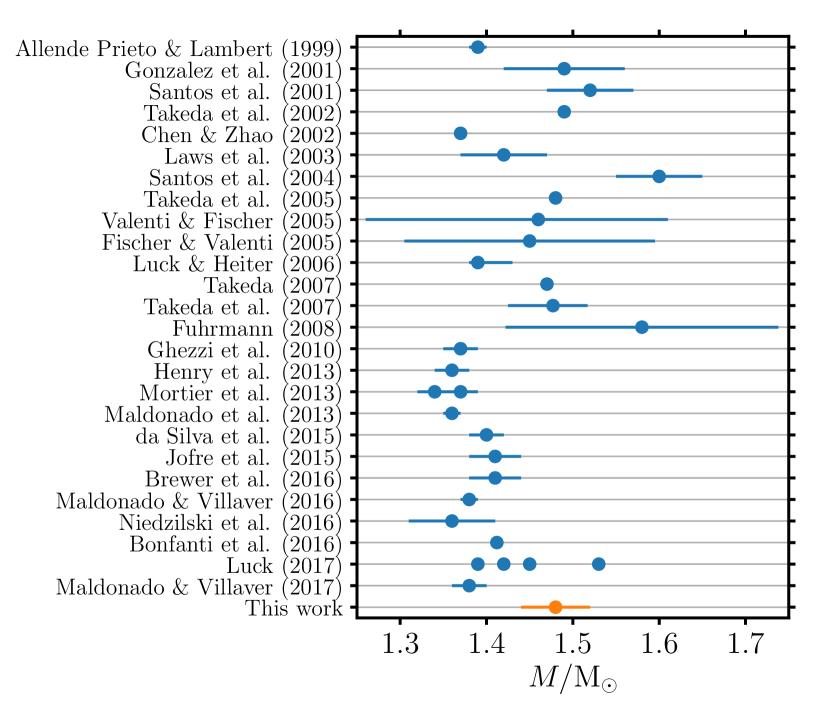
Figure 1: A selection of mass estimates for HD 38529 from the literature, as well as the estimate from this paper. Note that Mortier et al. (2013) reported two different values estimated using different line lists for the spectroscopic parameters. Luck (2017) reported values for four different sets of isochrones.

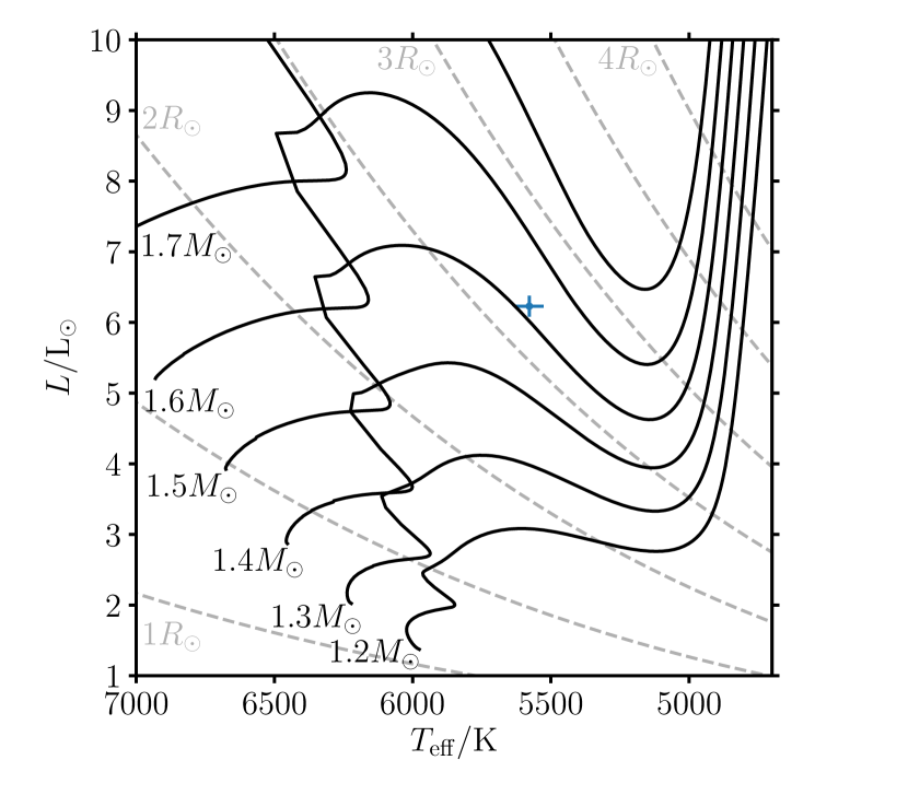
Figure 2: A Hertzsprung–Russell (HR) diagram showing the location of HD 38529 (blue point). The solid black lines show evolutionary tracks using the adopted metallicity $[\mathrm{Fe}/\mathrm{H}]=0.34\,\mathrm{dex}$ and masses from $1.2$ to $1.7\,\mathrm{M}_{\odot}$ in steps of $0.1\,\mathrm{M}_{\odot}$. The dashed grey lines are lines of constant radius from $1.0$ to $4.0\,\mathrm{R}_{\odot}$ in steps of $0.5\,\mathrm{R}_{\odot}$.

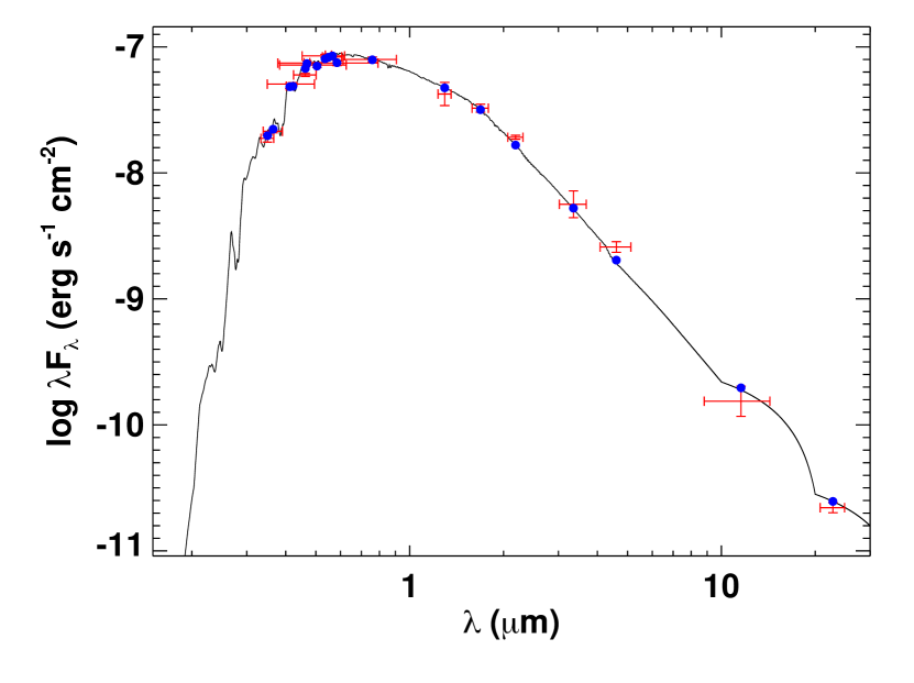
Figure 3: The spectral energy distribution (SED) of HD 38529. Data are indicated by red points and the best-fitting model by the solid black line. The blue points are the model’s integrated flux in the relevant filters.

Table 1: Spectroscopic measurements.

Source	$T_{\mathrm{eff}}/\,\mathrm{K}$	$[\mathrm{Fe}/\mathrm{H}]/\,\mathrm{dex}$	$\log g/\,\mathrm{dex}$
Deka-Szymankiewicz et al. (2018)	$5618\pm 15$	$0.38\pm 0.02$	$3.96\pm 0.04$
Maldonado & Villaver (2016)	$5585\pm 18$	$0.30\pm 0.02$	$3.86\pm 0.05$
Brewer et al. (2016)	$5541\pm 60$	$0.32\pm 0.06$	$3.77\pm 0.15$
Jofré et al. (2015)	$5573\pm 31$	$0.37\pm 0.05$	$3.81\pm 0.03$
Kang et al. (2011)	$5574\pm 74$	$0.32\pm 0.09$	$3.76\pm 0.10$
Adopted	$5578\pm 52$	$0.34\pm 0.06$	$3.83\pm 0.11$

2 Observations

2.1 Non-seismic

We assembled a list of spectroscopic parameters determined using different instruments and telescopes over the last ten years, summarised in Table 1. To combine these measurements into a set of representative values, we averaged the means and uncertainties and increased the uncertainties by the standard deviation of the means, in quadrature. This led to the adopted values of $T_{\mathrm{eff}}=5578\pm 52\,\mathrm{K}$, $[\mathrm{Fe}/\mathrm{H}]=0.34\pm 0.06\,\mathrm{dex}$ and $\log g=3.83\pm 0.11\,\mathrm{dex}$, though the asteroseismic observations constrain $\log g$ much more tightly than the spectroscopic value. The measurements from the individual sources are remarkably consistent, so the source of the parameters is not decisive in our stellar model fits. Fig. 2 shows the location of HD 38529 in a Hertzsprung–Russell (HR) diagram, using the luminosity derived in the next paragraph. HD 38529 is clearly a slightly evolved, metal-rich subgiant.

We derived a bolometric luminosity by fitting the spectral energy distribution (SED) using the methods described by Stassun & Torres (2016) and Stassun et al. (2017); Stassun et al. (2018). Photometry is available for photometric bands that cover wavelengths from $0.35$ to $22\mu\mathrm{m}$, as shown in Fig. 3. The specific sources are homogenised $UBV$ magnitudes from (Mermilliod, 2006), $B_{\mathrm{T}}V_{\mathrm{T}}$ magnitudes from Tycho-2 (Høg et al., 2000a, b), Strömgren $uvby$ magnitudes from (Paunzen, 2015), $JHK_{\mathrm{S}}$ magnitudes from 2MASS, $W1$–$4$ magnitudes from WISE (Wright et al., 2010), and Gaia’s $G$, $G_{BP}$ and $G_{RP}$ magnitudes. We fit the SED using the stellar atmosphere models by Kurucz (2013) with priors on the effective temperature $T_{\mathrm{eff}}$, surface gravity $\log g$ and metallicity $[\mathrm{Fe}/\mathrm{H}]$ from the spectroscopic values above. The extinction was fixed at zero because of the star’s small distance of $42.4\pm 0.1\,\mathrm{pc}$ implied by its Gaia DR2 parallax of $23.582\pm 0.059\,\mathrm{mas}$. Integrating the model SED gives a bolometric flux at the Earth $\mathcal{F}_{\mathrm{bol}}=(1.113\pm 0.026)\times 10^{-7}\,\mathrm{erg}\,\mathrm{s}^{-1}\,\mathrm{cm}^{-2}$, which, combined with the Gaia DR2 parallax, gives a bolometric luminosity $L=6.23\pm 0.15\,\mathrm{L}_{\odot}$. The best-fitting model is also shown in Fig. 3.

Baines et al. (2008) and Henry et al. (2013) both measured HD 38529’s angular size using CHARA, finding mutually-consistent limb-darkened angular sizes $\theta_{\mathrm{LD}}$ of $0.573\pm 0.049\,\mathrm{mas}$ and $0.593\pm 0.016\,\mathrm{mas}$, respectively. Given the Gaia DR2 parallax, these imply stellar radii of $2.61\pm 0.22\,\mathrm{R}_{\odot}$ and $2.70\pm 0.07\,\mathrm{R}_{\odot}$. Gaia DR2 includes a radius estimate of $2.81_{-0.21}^{+0.09}\,\mathrm{R}_{\odot}$, based on the $G$, $G_{BP}$ and $G_{RP}$ magnitudes (Andrae et al., 2018). The radius is degenerate with $L$ and $T_{\mathrm{eff}}$ when fitting our stellar models so we did not use it as a constraint, though we do compare our best-fitting radius with these independent values.

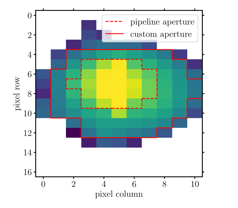
Figure 4: Median image of HD 38529 during TESS’s Sector 6 observations, with a logarithmic colour scale. The dashed and solid red lines show the default pipeline aperture and our custom aperture, respectively. White regions had negative median fluxes, which are possible because of the SPOC pipeline’s background subtraction.

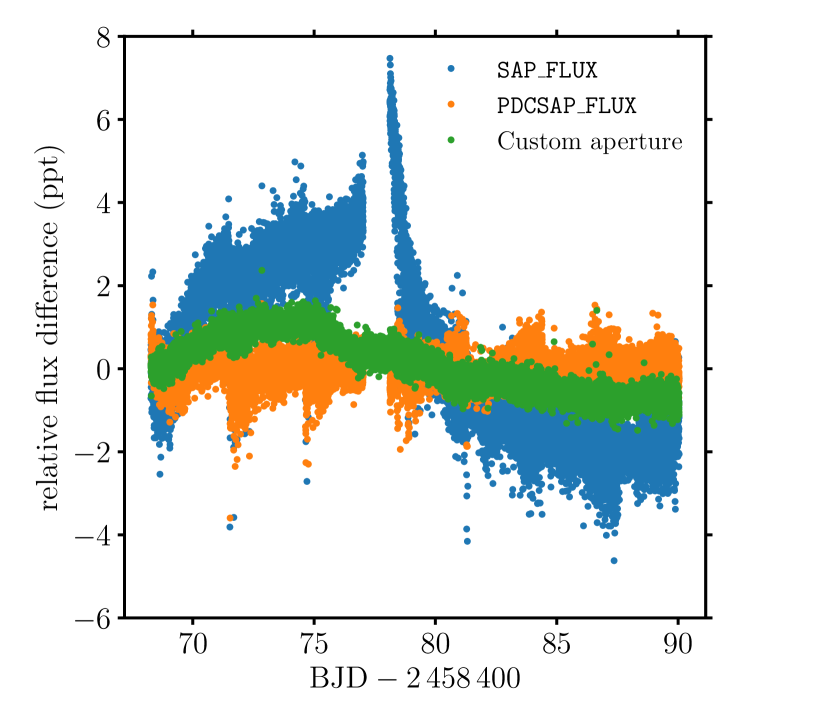
Figure 5: Lightcurves of HD 38529 using either the default pipeline’s SAP_FLUX or PDCSAP_FLUX data (blue or orange), compared with our custom, inpainted lightcurve (green).

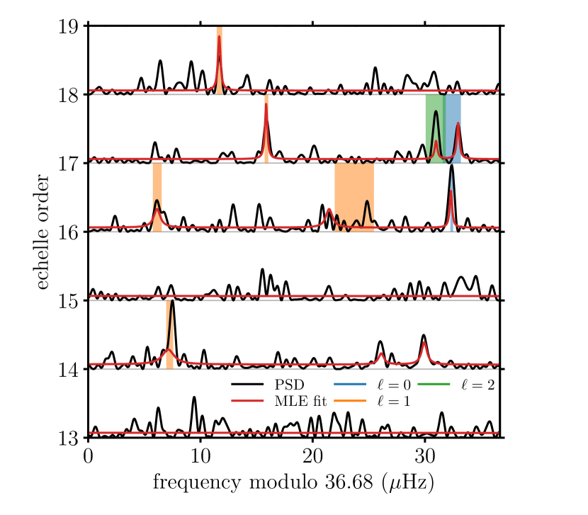
Figure 6: Échelle-like diagram of HD 38529 computed using the Lomb–Scargle periodogram on the custom lightcurve in Fig. 5 with an oversampling factor of 10. The periodogram is shown as a black curve, normalized to its maximum value between $400$ and $700\,\mu\mathrm{Hz}$. The blue, orange and green areas show the $1\sigma$ uncertainty ranges covered by the $\ell=0$, $1$ and $2$ mode frequencies given to the stellar modelling teams (see Table 2). The red curve is the MLE fit by the Birmingham team.

Table 2: Measured mode frequencies, all in $\,\mu\mathrm{Hz}$.

	Paris	Fort Myers	Birmingham	Adopted
$\ell$	UP+Asy.	Sig. test	MLE
$0$		$543.46$	$543.44\pm 0.23$
$0$	$583.47$		$583.61\pm 0.49$
$0$	$619.29$	$619.28$	$619.24\pm 0.12$	$619.27\pm 0.12$
$0$	$654.85$	$656.48$	$656.53\pm 0.21$	$655.95\pm 0.81$
$1$		$486.29$	$482.88\pm 0.63$
$1$	$520.81$	$520.65$	$520.89\pm 0.29$	$520.78\pm 0.31$
$1$	$592.98$	$592.88$	$593.22\pm 0.36$	$593.03\pm 0.39$
$1$	$611.72$	$611.70$	$608.37\pm 0.75$	$610.59\pm 1.74$
$1$	$639.43$	$639.45$	$639.44\pm 0.16$	$639.44\pm 0.16$
$1$	$671.99$	$671.91$	$671.90\pm 0.24$	$671.93\pm 0.24$
$2$	$539.55$		$539.55\pm 0.25$
$2$	$654.51$	$654.56$	$654.49\pm 0.89$	$654.52\pm 0.89$
$2$		$669.43$	$669.41\pm 0.29$

2.2 Seismic

HD 38529 was observed by TESS on its camera 1 during Sector 6 of Cycle 1 (2018 December 15 to 2019 January 6). We found no oscillations in the SPOC pipeline lightcurves (Jenkins et al., 2016) despite the star being among the top-ranked targets for asteroseismic detection in TESS’s Asteroseismic Target List (ATL, Schofield et al., 2019). We therefore computed a custom lightcurve in which we expanded the photometric aperture to include all pixels with a median flux greater than $10$ electrons per second ($\,\mathrm{e}^{-}\,\mathrm{s}^{-1}$). We found oscillations around roughly $600\,\mu\mathrm{Hz}$ in this custom lightcurve, though we note that the ATL predicted the oscillations would peak around $400\,\mu\mathrm{Hz}$.

To create a suitable lightcurve for subsequent analysis, we computed the total flux in apertures of different sizes. We considered flux thresholds starting from $10\,\mathrm{e}^{-}\,\mathrm{s}^{-1}$ for the largest aperture and increasing progressively in increments of $10\,\mathrm{e}^{-}\,\mathrm{s}^{-1}$, $50\,\mathrm{e}^{-}\,\mathrm{s}^{-1}$, $100\,\mathrm{e}^{-}\,\mathrm{s}^{-1}$ and $200\,\mathrm{e}^{-}\,\mathrm{s}^{-1}$, until reaching the standard TESS aperture, which is the smallest aperture studied (see González-Cuesta et al., in prep.). For all the apertures, we extracted the lightcurves and computed the power spectrum density (PSD). Our seismically-optimised aperture is the one where the oscillation modes’ signal-to-noise ratio is highest. We calibrated the lightcurve from the optimised aperture using the Kepler Asteroseismic Data Analysis Calibration Software (KADACS, García et al., 2011) that was developed and tested on Kepler data to remove outliers and correct jumps. Finally, we filled the gaps with the inpainting techniques by García et al. (2014) and Pires et al. (2015). For HD 38529, the optimal aperture was obtained with a flux threshold of $200\,\mathrm{e}^{-}\,\mathrm{s}^{-1}$.

The different apertures are shown in Fig. 4 and the lightcurves in Fig. 5. Both the standard pipeline lightcurves (SAP_FLUX and PDCSAP_FLUX) have increased scatter around the times of spacecraft thruster firings. With our larger aperture, more of the star’s light falls within the aperture during these motions, rather than being lost as bright parts of the star’s point spread function move in and out of the aperture.

Fig. 6 shows an échelle-like diagram of the power spectrum in the region that includes the detected oscillation modes, along with the individual mode frequencies that were used to model the star. The individual mode frequencies were measured from the power spectrum by three separate teams, which we identify by their affiliations, each using a different method. The first team (Paris) fit the universal pattern by Mosser et al. (2011) to identify the radial and quadrupole ($\ell=0$ and $2$) modes and the asymptotic expression by Mosser et al. (2015) to identify dipole ($\ell=1$) modes, selecting the nearest significant peaks in the power spectrum as the observed mode frequencies. The second team (Fort Myers) selected the peaks above a signal-to-noise ratio of 4 and the third team (Birmingham) used maximum-likelihood estimation (MLE) to fit Lorentzians to significant peaks in the power spectrum. The MLE fit is also shown in Fig. 6. Only the MLE fit returned straightforward uncertainties, which are derived from the inverse of the Hessian matrix of the fit.

To combine the various results, we conservatively selected mode frequencies only where all three teams reported a mode. Our adopted mean mode frequencies are the averages of the three teams’ frequency values. The adopted variances are the sum of the variances from the MLE fit and the variance of the three means. i.e., the adopted uncertainty is the sum, in quadrature, of the MLE uncertainty and the standard deviation of the three teams’ values. Table 2 lists all the mode frequencies identified by at least two teams as well as the adopted values that were provided to the stellar modellers.

The dipole modes are clearly mixed, i.e. the normally acoustic modes have coupled to gravity modes deep in the star’s interior, causing them to deviate from the nearly-regular spacing that is expected of purely acoustic modes. In particular, there are two dipole modes in échelle order $16$, which is only possible if the modes are mixed. Because mixed modes are partially sensitive to the properties of the stellar core, they have distinct diagnostic properties compared with purely acoustic modes.

Table 3: Stellar model settings for the different teams. The mixing-length parameter for the Birmingham models is a correction factor for the slight difference between the mixing-length formulations used in the stellar models and those used in the calibration by Mosumgaard et al. (2018).

Team	Aarhus	Birmingham	Porto
Models	GARSTECa	MESAb (r10398)	MESA (r9793)
Oscillations	ADIPLSc	GYREd	GYRE
High-$T$ opacities	OPALe	OPAL	OPAL
Low-$T$ opacities	F05f	F05	F05
EoS	OPALg	MESA/OPAL	MESA/OPAL
Solar mixture	AGSS09h	GN93i	GS98j
Helium law ($Y=\ldots$)	$0.25$–$0.34$	$1.289Z+0.248$	$2Z+0.248$
Nuclear reactions	NACREk+l,m	NACREk	NACREk+n,o
Atmosphere	Eddington	Mosumgaard et al. (2018)	Eddington
$\alpha_{\mathrm{MLT}}$	$1.5$–$2.1$	$1.037$*	$1.3$–$2.9$
Surface correction	BG14-1p	BG14-1	Sonoi et al. (2015)
Overshooting	None	Free	None
Team	Yale-M	Yale-Y
Models	MESA (r12115)	YREC
Oscillations	GYRE	Antia & Basu (1994)
High-$T$ opacities	OPAL	OPAL
Low-$T$ opacities	F05	F05
EoS	MESA/OPAL	OPAL
Solar mixture	GS98	GS98
Helium law ($Y=\ldots$)	$0.25$–$0.32$	$0.248$–$0.328$
Nuclear reactions	NACREk	Solar fusion Iq
Atmosphere	Eddington	Eddington
$\alpha_{\mathrm{MLT}}$	$1.83$	$1.6$–$2.2$
Surface correction	BG14-2	BG14-2
Overshooting	None	$U(0,0.4)$

aWeiss & Schlattl (2008)	bPaxton et al. (2011); Paxton et al. (2013, 2015)	cChristensen-Dalsgaard (2008)
dTownsend & Teitler (2013); Townsend et al. (2018)	eIglesias & Rogers (1993, 1996)	fFerguson et al. (2005)
gRogers & Nayfonov (2002)	hAsplund et al. (2009)	iGrevesse & Noels (1993)
jGrevesse & Sauval (1998)	kAngulo et al. (1999)	lFormicola et al. (2004)
mHammer et al. (2005)	nImbriani et al. (2005)	oKunz et al. (2002)
pBall & Gizon (2014)	qAdelberger et al. (1998)

3 Stellar modelling

Five teams, identified by their affiliations, analysed HD 38529 using a variety of stellar evolution and oscillation codes, with a range of choices for various physical properties (sometimes referred to as input physics). The main choices are shown in Table 3. In the rest of this section, we briefly comment on some notable choices and describe the procedures that each team used to find best-fitting model parameters and uncertainties.

The oscillation mode frequencies of calibrated solar models are known to differ systematically from those of the Sun because of poor modelling of the near-surface layers. These differences, known as surface effects (see Ball, 2017, for a review), presumably affect all solar-like oscillators and must therefore be corrected or removed to obtain unbiased model parameters. All the teams here have applied existing formulae to the uncorrected model frequencies $\nu_{\mathrm{uncorr},i}$ to create the corrected model frequencies $\nu_{\mathrm{corr},i}$ that are then compared with the data. Other methods can be used when no modes are mixed and more mode frequencies are measured (e.g. Roxburgh & Vorontsov, 2003; Roxburgh, 2015, 2016).

All teams combine the $\chi^{2}$ contributions of different observations, for which it is useful to define the $\chi^{2}$ contribution of a particular quantity $q$ by

$$\chi^{2}_{q}=\left(\frac{q_{\mathrm{obs}}-q_{\mathrm{mdl}}}{\sigma_{q}}\right)^{2}\mathrm{,}$$ (1)

where $q_{\mathrm{obs}}$, $q_{\mathrm{mdl}}$ and $\sigma_{q}$ are the observed value, modelled value and observed uncertainty for the quantity $q$. In addition, many teams used the total $\chi^{2}$ of the oscillation mode frequencies,

$$\chi^{2}_{\mathrm{seis}}=\sum_{i=1}^{N_{\mathrm{seis}}}\left(\frac{\nu_{\mathrm{obs}}-\nu_{\mathrm{corr},i}}{\sigma_{\nu_{i}}}\right)^{2}\mathrm{,}$$ (2)

where $N_{\mathrm{seis}}=8$ is the total number of observed modes and $\nu_{\mathrm{corr},i}$ is the $i$th surface-corrected model frequency. We also define the contribution of the non-seismic observations by

$$\chi^{2}_{\mathrm{non-seis}}=\chi^{2}_{[\mathrm{Fe}/\mathrm{H}]}+\chi^{2}_{T_{\mathrm{eff}}}+\chi^{2}_{L}\mathrm{.}$$ (3)

We note that, as is common in one-dimensional stellar evolution codes, none of the models included the potentially relevant effects of rotation or radiative levitation, which we comment on further in Sec. 4.2. Only the Yale-Y team used any gravitational settling.

3.1 Aarhus

The Aarhus team used the Bayesian fitting code BASTA (Silva Aguirre et al., 2015, 2017) to sample stellar models on a pre-computed grid. The grid spanned masses from $1.30$ to $1.60\,\mathrm{M}_{\odot}$, mixing-length parameters $\alpha_{\mathrm{MLT}}$ from $1.5$ to $2.1$, initial metallicities $[\mathrm{Fe}/\mathrm{H}]$ from $0.2$ to $0.5\,\mathrm{dex}$ and initial helium abundances from $0.25$ to $0.34$. The parameters were sampled with 5000 evolutionary tracks selected by Sobol quasi-random sampling. BASTA uses Bayesian inference to compute the marginalised posterior of any stellar quantity by integrating over all models and applying weights to handle non-uniform sampling in the volume of the parameter space. For example, more models are computed during rapid phases of evolution. Without weights, the results would be biased towards these rapid phases, so a weight is applied to avoid this. The value reported for each quantity is the median of the posterior with the 16th and 84th percentiles. The objective function is the likelihood $\mathcal{L}\propto\exp(-\chi^{2}_{\mathrm{tot}}/2)$, with

$$\chi^{2}_{\mathrm{tot}}=\frac{1}{N_{\mathrm{seis}}-1}\chi^{2}_{\mathrm{seis}}+\chi^{2}_{\mathrm{non-seis}}\mathrm{.}$$ (4)

As the star evolves and the modes become mixed, multiple non-radial modes ($\ell>0$) can occur between two consecutive radial ($\ell=0$) modes. To decide which modes in the model should be included in the likelihood function, BASTA matches the modes in the models to the observed modes based on their separation in frequency as well as the mode inertias (Aerts et al., 2010).

For a given angular degree $\ell>0$, suppose there are $n>1$ modelled modes between two radial modes, and that these non-radial modes have inertias $I_{1}<\ldots<I_{n}$. We possibly do not observe all the modes between the radial modes so have some number $m\leq n$ of observed modes, and must somehow choose which $m$ modelled modes to compare to the observed modes. The simplest method is to select the modelled modes with the lowest inertias, as these are expected to have the highest amplitudes, but small differences in inertia might lead to an incorrect selection.

Instead BASTA creates two inertia thresholds $a=I_{m}/10$ and $b=10\,I_{m}$, where $I_{m}$ is the $m$th-smallest inertia of the modelled modes between the two radial modes. It then subdivides the modelled modes into a set $A$ with inertias less than $a$, set $B$ with inertias between $a$ and $b$, and set $C$ with inertias greater than $b$. These thresholds roughly distinguish modes that are likely to be detected (set $A$), those that are unlikely to be detected (set $C$) and those somewhere between (set $B$). The values of $a$ and $b$ ensure that $A$ has fewer than $m$ elements and $A\cup B$ has at least $m$ elements. These thresholds are determined from experience and have led to robust results in all their applications so far. By selecting all modes in $A$ and a subset of $B$ such that $m$ modes are chosen in total, the modes can be matched one-to-one to the observed modes. If there are no modes in $A$, all the modes are selected from $B$. To decide which modes to select from $B$, BASTA uses the subset of $B$ with the smallest total absolute frequency difference between the observed and modelled modes (i.e. the $\mathrm{L}_{1}$ norm).

3.2 Birmingham

The Birmingham team used Modules for Experiments in Stellar Astrophysics (MESA, r10398; Paxton et al., 2011; Paxton et al., 2013, 2015) with the atmosphere models and calibrated mixing-length parameters from Trampedach et al. (2014a, b) as implemented in Mosumgaard et al. (2018). The mixing-length parameter in Table 3 is the solar-calibrated correction factor that accommodates slight differences between MESA’s input physics and mixing-length model and that of the simulations by Trampedach et al. (2014a, b). All other teams used grey Eddington atmosphere models.

The Birmingham team optimised the mass $M$, initial metallicity $[\mathrm{Fe}/\mathrm{H}]_{i}$, overshoot parameter $\alpha_{\mathrm{ov}}$ and age $t$ to minimise the unweighted total squared differences between the model and both the seismic and non-seismic data, i.e.

$$\chi^{2}_{\mathrm{tot}}=\chi^{2}_{\mathrm{seis}}+\chi^{2}_{\mathrm{non-seis}}\mathrm{.}$$ (5)

The overshooting parameter $\alpha_{\mathrm{ov}}$ is the number of pressure scale-heights that are chemically mixed beyond the formal convective boundaries. The team optimised the parameters using a combination of a downhill simplex (i.e. Nelder–Mead method, Nelder & Mead, 1965) and samples drawn randomly within error ellipses around the best-fitting parameters when the simplex stagnated. Uncertainties were estimated by finding the parameters of minimum-volume ellipsoids that simultaneously bound all samples with $0.25<\chi^{2}_{\mathrm{tot}}-\mathrm{min}(\chi^{2}_{\mathrm{tot}})<25$ when their distance to the optimum is scaled by $\sqrt{\chi^{2}_{\mathrm{tot}}}$, as described by Ball & Gizon (2017).

3.3 Porto

The Porto team used the software package Asteroseimic Inference on a Massive Scale (AIMS, Rendle et al., 2019), which interpolates stellar properties in a precomputed grid and estimates parameters and their uncertainties by Markov Chain Monte Carlo (MCMC) sampling of a chosen posterior distribution.

The sampled posterior comprises uniform priors in appropriate ranges and a likelihood function defined as $\mathcal{L}\propto\exp(-\chi^{2}_{\mathrm{tot}}/2)$, where

$$\chi^{2}_{\mathrm{tot}}=\frac{3}{N_{\mathrm{seis}}}\chi^{2}_{\mathrm{seis}}+\chi^{2}_{\mathrm{non-seis}}\mathrm{,}$$ (6)

where the factor $3$ is used to balance the seismic constraints with the three non-seismic constraints.

For HD 38529, the posterior distributions appear to be dominated by a single stellar model in the underlying grid, with a limited contribution from a few other models and interpolation around those models. To compute more reliable uncertainties, we use the points at which the cumulative distribution functions are equal to $0.0013$ and $0.9987$, and divide this range by three. These points correspond to the $3\sigma$ limits of a normal distribution, in the same way that the 16th and 84th percentiles correspond to the $1\sigma$ limits.

3.4 Yale-M

The Yale-M team used the parallel differential evolution algorithm by Tasoulis et al. (2004) as implemented in the Python package Yabox (Mier, 2017) to find the optimal values of the mass, initial helium abundance and initial metallicity. The mass was allowed to vary between $1.39$ and $1.61\,\mathrm{M}_{\odot}$, the initial helium abundance between $0.25$ and $0.32$ and the initial metal-to-hydrogen ratio $Z/X$ between $0.038$ and $0.05$, which were chosen based on an initial rough optimisation using only the radial mode frequencies and non-seismic constraints.

The objective function is a total sum of squared differences $\chi^{2}_{\mathrm{tot}}$, defined by

$$\chi^{2}_{\mathrm{tot}}=\frac{1}{N_{\mathrm{seis}}}\chi^{2}_{\mathrm{seis}}+\chi^{2}_{\mathrm{3}}+\chi^{2}_{\mathrm{non-seis}}$$ (7)

with

$$\chi^{2}_{\mathrm{3}}=\frac{1}{3}\sum_{i=1}^{3}\chi^{2}_{\nu_{\mathrm{uncorr},i}}\mathrm{,}$$ (8)

where $\nu_{\mathrm{uncorr},i}$ is the uncorrected model frequency. The extra term $\chi^{2}_{\mathrm{3}}$ is the reduced $\chi^{2}$ of the three lowest frequency modes, before correction, which acts as a prior that prefers those models for which the three lowest uncorrected mode frequencies are similar to the observed mode frequencies.

All the models generated by the differential evolution were retained, which in effect created a non-uniform grid of models. The density of models in each region of parameter space was sampled using a kernel density estimator (KDE), which defines a prior for how likely each model was in the absence of any observations. The total $\chi^{2}_{\mathrm{tot}}$ was then transformed into a likelihood $\mathcal{L}\propto\exp(-\chi^{2}_{\mathrm{tot}}/2)$ from which the means and standard deviations could be estimated from the moments of the resulting formal posterior distribution.

3.5 Yale-Y

The Yale-Y team constructed a grid of models spanning masses from $1.40$ to $1.60\,\mathrm{M}_{\odot}$ in steps of $0.01\,\mathrm{M}_{\odot}$, mixing length parameters $\alpha_{\mathrm{MLT}}$ from $1.6$ to $2.2$ in steps of $0.075$, initial helium abundances $Y_{i}$ from $0.248$ to $0.328$ in steps of $0.01$ and initial metallicities $[\mathrm{Fe}/\mathrm{H}]_{i}$ from $0.260$ to $0.390\,\mathrm{dex}$ in steps of $0.015\,\mathrm{dex}$.

Each model had a random core overshoot parameter $\alpha_{\mathrm{ov}}$ selected uniformly between $0$ and $0.4$, with overshooting modelled in the same way as the Birmingham team. The models included gravitational settling, with an efficiency multiplied by the factor $\exp[-(1/2)(M/\,\mathrm{M}_{\odot}-1.25)^{2}/0.085^{2}]$ to prevent the heavy elements from completely draining from the surface during the main-sequence (see Sec. 4.2).

The relative likelihood of each model was computed using $\mathcal{L}\propto\exp(-\chi^{2}_{\mathrm{tot}}/2)$, with

$$\chi^{2}_{\mathrm{tot}}=\frac{1}{N_{\mathrm{seis}}}\chi^{2}_{\mathrm{seis}}+\chi^{2}_{\mathrm{non-seis}}\mathrm{.}$$ (9)

The reported values are the medians and 16th and 84th percentiles of the likelihoods marginalised over all other parameters.

Table 4: Best-fitting stellar model parameters.

Team	$M/\,\mathrm{M}_{\odot}$	$R/\,\mathrm{R}_{\odot}$	$t/\,\mathrm{Gyr}$	$L/\,\mathrm{L}_{\odot}$	$\bar{\rho}/(\mathrm{g}\,\mathrm{cm}^{3})$
Aarhus	$1.480_{-0.031}^{+0.067}$	$2.677_{-0.027}^{+0.037}$	$3.17_{-0.16}^{+0.10}$	$6.11_{-0.10}^{+0.20}$	$0.1094_{-0.0003}^{+0.0003}$
Birmingham	$1.439\pm 0.024$	$2.653\pm 0.017$	$3.29\pm 0.08$	$6.00\pm 0.09$	$0.1085\pm 0.0006$
Porto	$1.492\pm 0.007$	$2.686\pm 0.006$	$2.89\pm 0.03$	$6.32\pm 0.11$	$0.1085\pm 0.0006$
Yale-M	$1.498\pm 0.047$	$2.691\pm 0.029$	$2.81\pm 0.02$	$6.18\pm 0.08$	$0.1083\pm 0.0003$
Yale-Y	$1.489\pm 0.030$	$2.685\pm 0.024$	$3.20\pm 0.74$	$6.17\pm 0.15$	$0.1065\pm 0.0012$
Adopted	$1.479\pm 0.037$	$2.678\pm 0.026$	$3.07\pm 0.39$	$6.16\pm 0.15$	$0.1083\pm 0.0012$

4 Results and Discussion

The stellar parameter values inferred by each team are given in Table 4, along with consolidated parameter values. The consolidated values are computed by combining the results from each team using the same method as for the spectroscopic data. The main results are the mass $M=1.48\pm 0.04\,\mathrm{M}_{\odot}{}$, radius $R=2.68\pm 0.03\,\mathrm{R}_{\odot}{}$ and age $t=3.07\pm 0.39\,\mathrm{Gyr}{}$. The mass is near the upper end of the range of masses that have appeared in the literature and similar to the value $1.48\pm 0.05\,\mathrm{M}_{\odot}$ determined by Takeda et al. (2007) and used by Benedict et al. (2010). The radius is measured more precisely than in any previous study and our result is consistent with both the Gaia DR2 value (Andrae et al., 2018) and the interferometric measurements by Baines et al. (2008) and Henry et al. (2013) when combined with the Gaia DR2 parallax.

A sixth team independently calibrated a stellar model to the spectroscopic data and radial frequencies only and found a consistent mass $M=1.48\,\mathrm{M}_{\odot}$, radius $R=2.68\,\mathrm{R}_{\odot}$ and age $t=2.70\,\mathrm{Gyr}$. This model also used MESA (r10000), ADIPLS, the solar mixture of Asplund et al. (2009), the surface correction by Kjeldsen et al. (2008) and input physics otherwise similar to that of the Porto and Yale-M teams.

4.1 Precise age estimates

Several of the pipeline’s age estimates appear unreasonably precise. As a reference, we first note that the uncertainty on any single evolutionary track is very small because of how quickly the mode frequencies change with age (see Deheuvels & Michel, 2011, for a detailed discussion). In HD 38529, the dipole modes can change at about $3\,\mu\mathrm{Hz}/\,\mathrm{Myr}$ and the fastest changing mode takes about $0.1\,\mathrm{Myr}$ to evolve by $1\sigma$. The reported age uncertainties are therefore dominated by the correlation of age with other parameters, notably the mass. A star’s main-sequence lifetime is roughly proportional to $M^{-3}$, so we roughly expect the fractional age uncertainty to be about $3$ times the fractional mass uncertainty, though this does not account for correlations with other parameters. The Birmingham team’s estimate is about half this value and the Yale-M team’s estimate even smaller, even though the other parameter uncertainties seem reasonable. e.g. because the mean density $\bar{\rho}$ is very tightly constrained, the fractional uncertainty on mass is about $3$ times that of the radius.

Such precise ages for subgiants and low-luminosity red giants have been encountered before (e.g. Deheuvels & Michel, 2011; Ball & Gizon, 2017; Stokholm et al., 2019; Li et al., 2020) but in most cases, the mass uncertainties are sufficiently precise that the age uncertainties are still consistent. We note, however, that Stokholm et al. (2019) inferred very precise ages for the bright subgiant HR 7322 (KIC 10005473) and discuss the constraining power of its mixed modes in detail. Li et al. (2020) also report age uncertainties that are more precise than the naïve estimate for the stars KIC 6766513, KIC 7199397, KIC 10147635, KIC 11193681 and KIC 11771760. There is no obvious connection between these stars other than their best-fitting masses all being greater than $1.3\,\mathrm{M}_{\odot}$. We also note that, at least in the Birmingham team’s models, the dipole-mode frequencies are all increasing while the star’s radius is staying roughly constant, as Stokholm et al. (2019) also found for HR 7322. Because the star’s mean density is therefore roughly constant, one would expect purely acoustic mode frequencies to be roughly constant too. That the dipole-mode frequencies are increasing implies that they are undergoing avoided crossings driven by changes to the star’s internal structure, which might reduce the correlation with other parameters that should dominate the age uncertainty.

It is not clear how additional free parameters (e.g. the initial helium abundance $Y_{i}$ or mixing length parameter $\alpha_{\mathrm{MLT}}$) affect the age uncertainties. It is possible for certain combinations of parameters to be required for better fits to the data, which could confine the age by having it (anti)correlate with multiple parameters such that the simple estimate here—which assumes no correlations—is an overestimate. Even so, the more uncertain estimate by the Yale-Y team and the extra uncertainty from the spread of means (which contributes about $0.2\,\mathrm{Gyr}$) means that our overall result is less certain than the lower bound suggested by the simple relationship between mass and age.

4.2 Neglected transport mechanisms

HD 38529’s mass places it in a region where stellar models typically neglect several potentially important processes that can transport chemical species in the star. On the other hand, HD 38529 has evolved far enough that the inward movement of the convective envelope’s inner boundary will have already erased the signal of some chemical peculiarities that may have existed while the star was on the main sequence. At this point in the star’s evolution, roughly the outer half by mass is convective. Even so, the extra chemical transport processes may have affected the structure of the star in ways that still affect its observable appearance.

The first such process is rotation. HD 38529 would have been an early- to mid-F-type star ($T_{\mathrm{eff}}\approx 6700\,\mathrm{K}$) on the main-sequence, so may have rotated relatively quickly. Measurements of the star’s current $v\sin i$ in the literature show a large spread, so we use the estimate of the rotation period $P=31.65\pm 0.17\,\mathrm{d}$ by Benedict et al. (2010) based on photometry from the Hubble Space Telescope’s Fine Guidance Sensor. We note that they report an amplitude of $0.15$ per cent for the rotational modulation, in which case the amplitude and period are consistent with the roughly sinusoidal variation in our custom TESS lightcurve.

Though our understanding of angular momentum transport in evolved stars has been shown to lack some important process (Eggenberger et al., 2012; Marques et al., 2013), the star’s surface gravity $\log g\approx 3.75\,\mathrm{dex}$ places it around the point at which the radial rotation profiles appear to first depart from solid-body rotation (see e.g. Deheuvels et al., 2014; Spada et al., 2016). The star’s main-sequence radius grew from about $1.4\,\mathrm{R}_{\odot}$ at zero age to about $2.1\,\mathrm{R}_{\odot}$ at terminal age so, assuming solid body rotation, its rotation period would have increased from about $8.5$ to $19.1\,\mathrm{d}$. Equivalently, the rotational velocity decreased from about $8.4$ to $5.6\,\mathrm{km}\,\mathrm{s}^{-1}$. It is thus unlikely that HD 38529 rotated quickly on the main sequence, so the chemical transport by rotation was probably modest.

The second process we have neglected (or, for the Yale-Y team, suppressed) is chemical diffusion, which describes the separate processes of gravitational settling and radiative levitation (Michaud et al., 2015). As is common when modelling stars more massive than about $1.2$ to $1.3\,\mathrm{M}_{\odot}$, we have neglected or suppressed gravitational settling because current models predict that heavier elements are completely drained from the stellar surface, which is clearly at odds with observations. It is usually assumed that some competing transport process prevents this from happening but its precise nature is still unknown (see e.g. Sec. 6.2 of Salaris & Cassisi, 2017).

Radiative levitation is a related process that raises heavier elements towards the stellar atmosphere because they are subject to a greater radiative force against gravity than lighter elements. Deal et al. (2018) showed that this is an important process when inferring the properties of main-sequence stars. Deal et al. (2020) further showed that modest rotation (about $30\,\mathrm{km}\,\mathrm{s}^{-1}$) is insufficient to prevent a discernible effect on the stellar properties. Given that HD 38529 probably rotated more slowly, it may have experienced significant heavy element enhancement at its surface on the main sequence, even if much of the effect has since been erased by the growing convective envelope.

To roughly quantify the effect of these neglected processes, we first computed evolutionary tracks up to the observed $T_{\mathrm{eff}}=5578\,\mathrm{K}$ with $M=1.48\,\mathrm{M}_{\odot}$, $[\mathrm{Fe}/\mathrm{H}]=0.34$ and a rotation rate of $5\,\mathrm{d}$ at age $10\,\mathrm{Myr}$ as described in Deal et al. (2020). Each track used one of the following combinations of the extra chemical transport processes above: rotation, gravitational settling and radiative levitation; gravitational settling and radiative levitation; only gravitational settling; and no extra chemical transport. The tracks show that gravitational settling leads to a longer main-sequence lifetime and a brighter subgiant phase, which in turn suggests that we have overestimated the star’s mass and underestimated its age. Radiative levitation appears to have little effect on the main-sequence evolution and any abundance anomalies are erased by the convection zone on the subgiant branch.

We then varied the input mass of the tracks with rotation, gravitational settling and radiative levitation to find a model that reached the same values of $\log g$ and $T_{\mathrm{eff}}$ as the $1.48\,\mathrm{M}_{\odot}$ track with no extra chemical transport. The best-fitting model by this approximate method has a mass of $1.395\,\mathrm{M}_{\odot}$ and is $31$ per cent older than the $1.48\,\mathrm{M}_{\odot}$ model without extra chemical transport. From the constraint of fixed $\log g$, the radius is about $3.0$ per cent smaller, which is roughly a $3.1\sigma$ difference. The mass, radius and age therefore differ by about $2.4$, $3.1$ and $2.5\sigma$, respectively, when using our reported fractional uncertainties. Though this analysis only varies the mass and age and does not use any seismic constraints, it demonstrates the potential importance of gravitational settling and rotation when determining the properties of stars like HD 38529.

4.3 Implications for companion brown dwarf

As noted earlier, HD 38529 hosts a planet and brown dwarf, and our results present a number of implications for these companions. Luhn et al. (2019) provide the most recent measurements and used a host mass of $1.41\,\mathrm{M}_{\odot}$ determined by Brewer et al. (2016). The companion masses scale with $M^{2/3}$ so our inferred mass implies that the companions are $3.2$ per cent larger than Luhn et al. (2019) report.

Our revised stellar properties affect the extent of the habitable zone (HZ, e.g. Kasting et al., 1993; Kopparapu et al., 2013, 2014) around HD 38529. Kane et al. (2016) defined “conservative” (based on runaway and maximum greenhouse models) and “optimistic” (based on empirical data from Venus and Mars) HZ boundaries, both of which are sensitive to small changes in stellar properties and their associated uncertainties (Kane, 2014). Our radius of $2.68\pm 0.03\,\mathrm{R}_{\odot}{}$ and adopted effective temperature of $5578\pm 52\,\mathrm{K}$ (see Sec. 2.1) result in calculated ranges of $2.40$–$4.26\,\mathrm{AU}$ and $1.90$–$4.50\,\mathrm{AU}$ for the conservative and optimistic HZ boundaries, respectively. The outer companion, with a semi-major axis $3.70\pm 0.03\,\mathrm{AU}$, periastron $2.44\pm 0.03\,\mathrm{AU}$ and apastron $4.96\pm 0.05\,\mathrm{AU}$, spends most of its orbit in the HZ by either definition, and might host habitable moons (Hinkel & Kane, 2013; Hill et al., 2018).

The strong degeneracies between age, mass and luminosity make brown dwarfs with independent age estimates invaluable benchmarks for testing models of substellar evolution (e.g. Marley & Robinson, 2015; Bowler, 2016). While the expected separation ($\sim 70\,\mathrm{mas}$) and contrast ($\sim 10^{-7}$) between HD 38529 and its brown dwarf companion are beyond the capabilities of current adaptive optics instruments to measure the brown dwarf’s luminosity and thus test stellar models directly, we can use the asteroseismic age of the primary to constrain its expected properties. For example, linearly interpolating the models by Baraffe et al. (2003) using the mass reported by Luhn et al. (2019), increased by 3.2 per cent to account for our higher estimate of the star’s mass, and our age constraint of $3.07\pm 0.39\,\mathrm{Gyr}{}$ yields $T_{\mathrm{eff}}\approx 560\,\mathrm{K}$, $R\approx 0.985\,\mathrm{R}_{\mathrm{J}}$ and $\log_{10}(L/\,\mathrm{L}_{\odot})\approx-6.13$, consistent with a Y-dwarf near the planetary mass boundary.

5 Conclusions

We have measured robust asteroseismic properties for the planet host HD 38529 by analysing its solar-like oscillations from TESS and complementary non-seismic parameters with five different stellar modelling pipelines. We infer a stellar mass $M=1.48\pm 0.04\,\mathrm{M}_{\odot}{}$, radius $R=2.68\pm 0.03\,\mathrm{R}_{\odot}{}$ and age $t=3.07\pm 0.39\,\mathrm{Gyr}{}$. Our mass measurement is near the upper end of the range that has appeared in the literature. Our radius measurement is consistent with the Gaia DR2 and previous interferometric values, when combined with the new Gaia parallax measurement.

It is unclear how much more can be extracted from the asteroseismology of HD 38529. Though TESS will observe the Southern hemisphere again in its Cycle 3, HD 38529 will narrowly miss being re-observed, falling in the gap between Sectors 32 and 33 according to the currently planned satellite pointings. A more advanced reduction of the existing photometry, however, might raise several more oscillation modes above the noise level. Five additional oscillations modes in Table 2 were identified by two of the three methods. If these were all robustly detected, the substantial increase in seismic data could warrant a new analysis that would yield a more detailed picture of the star’s properties.

Nevertheless, our results demonstrate that precise stellar parameters can be recovered from relatively poor asteroseismic observations. Despite measuring only eight oscillation mode frequencies, we have measured the mass and radius to within $2.7$ and $1.1$ per cent, which are within the limits of 2 and 15 per cent required for PLATO’s core scientific objectives (Goupil, 2017). Our age estimate is slightly less precise ($13.6$ per cent) than PLATO’s requirement of 10 per cent for main-sequence stars. The longer duration of PLATO’s observations should provide more precise frequency estimates, even in cases where few modes are detected, so our results suggest that PLATO’s requirements can be met in relatively faint subgiants ($G\approx 11$). Above all, our results imply that TESS has itself observed many more stars that are interesting (aside from their oscillations) and could be analysed asteroseismically, even if the seismic data appears poor.

Data availability

Original TESS lightcurves and pixel-level data are available from the Mikulski Archive for Space Telescopes at http://mast.stsci.edu/. Other data underlying this article will be shared on reasonable request to the corresponding author.

References

- Adelberger et al. (1998) Adelberger E. G., et al., 1998, Reviews of Modern Physics, 70, 1265
- Aerts et al. (2010) Aerts C., Christensen-Dalsgaard J., Kurtz D. W., 2010, Asteroseismology. Astronomy and Astrophysics Library, Springer, Berlin
- Allende Prieto & Lambert (1999) Allende Prieto C., Lambert D. L., 1999, A&A, 352, 555
- Andrae et al. (2018) Andrae R., et al., 2018, A&A, 616, A8
- Angulo et al. (1999) Angulo C., et al., 1999, Nuclear Physics A, 656, 3
- Antia & Basu (1994) Antia H. M., Basu S., 1994, A&AS, 107, 421
- Asplund et al. (2009) Asplund M., Grevesse N., Sauval A. J., Scott P., 2009, ARA&A, 47, 481
- Baglin et al. (2006) Baglin A., Auvergne M., Barge P., Deleuil M., Catala C., Michel E., Weiss W., COROT Team 2006, in Fridlund M., Baglin A., Lochard J., Conroy L., eds, ESA Special Publication Vol. 1306, ESA Special Publication. p. 33
- Baines et al. (2008) Baines E. K., McAlister H. A., ten Brummelaar T. A., Turner N. H., Sturmann J., Sturmann L., Goldfinger P. J., Ridgway S. T., 2008, ApJ, 680, 728
- Ball (2017) Ball W. H., 2017, in European Physical Journal Web of Conferences. p. 02001 (arXiv:1711.01271), doi:10.1051/epjconf/201716002001
- Ball & Gizon (2014) Ball W. H., Gizon L., 2014, A&A, 568, A123
- Ball & Gizon (2017) Ball W. H., Gizon L., 2017, A&A, 600, A128
- Baraffe et al. (2003) Baraffe I., Chabrier G., Barman T. S., Allard F., Hauschildt P. H., 2003, A&A, 402, 701
- Benedict et al. (2010) Benedict G. F., McArthur B. E., Bean J. L., Barnes R., Harrison T. E., Hatzes A., Martioli E., Nelan E. P., 2010, AJ, 139, 1844
- Bonfanti et al. (2016) Bonfanti A., Ortolani S., Nascimbeni V., 2016, A&A, 585, A5
- Borucki et al. (2010) Borucki W. J., et al., 2010, Science, 327, 977
- Bowler (2016) Bowler B. P., 2016, PASP, 128, 102001
- Brewer et al. (2016) Brewer J. M., Fischer D. A., Valenti J. A., Piskunov N., 2016, ApJS, 225, 32
- Campante et al. (2019) Campante T. L., et al., 2019, ApJ, 885, 31
- Chen & Zhao (2002) Chen Y.-Q., Zhao G., 2002, Chinese J. Astron. Astrophys., 2, 151
- Christensen-Dalsgaard (2008) Christensen-Dalsgaard J., 2008, Ap&SS, 316, 113
- CoRot Team (2016) CoRot Team 2016, The CoRoT Legacy Book: The adventure of the ultra high precision photometry from space, by the CoRot Team. EDP Sciences, doi:10.1051/978-2-7598-1876-1
- Deal et al. (2018) Deal M., Alecian G., Lebreton Y., Goupil M. J., Marques J. P., LeBlanc F., Morel P., Pichon B., 2018, A&A, 618, A10
- Deal et al. (2020) Deal M., Goupil M. J., Marques J. P., Reese D. R., Lebreton Y., 2020, A&A, 633, A23
- Deheuvels & Michel (2011) Deheuvels S., Michel E., 2011, A&A, 535, A91
- Deheuvels et al. (2014) Deheuvels S., et al., 2014, A&A, 564, A27