A Study in Frequency-Dependent Effects on Precision Pulsar Timing Parameters with the Pulsar Signal Simulator

Abstract

In this paper we introduce a new python package, the Pulsar Signal Simulator, or psrsigsim, which is designed to simulate a pulsar signal from emission at the pulsar, through the interstellar medium, to observation by a radio telescope, and digitization in a standard data format. We use the psrsigsim to simulate observations of three millisecond pulsars, PSRs J1744–1134, B1855+09, and B1953+29, to explore the covariances between frequency-dependent parameters, such as variations in the dispersion measure (DM), pulse profile evolution with frequency, and pulse scatter broadening. We show that the psrsigsim can produce realistic simulated data and can accurately recover the parameters injected into the data. We also find that while there are covariances when fitting DM variations and frequency-dependent parameters, they have little effect on timing precision. Our simulations also show that time-variable scattering delays decrease the accuracy and increase the variability of the recovered DM and frequency-dependent parameters. Despite this, our simulations also show that the time-variable scattering delays have little impact on the root mean square of the timing residuals. This suggests that the variability seen in recovered DM, when time-variable scattering delays are present, is due to a covariance between the two parameters, with the DM modeling out the additional scattering delays.

1 Introduction

Precision timing of millisecond pulsars (MSPs) has allowed us to study some of the most extreme astrophysical phenomena, from the equations of state of neutron stars (e.g., Antoniadis et al., 2013; Stovall et al., 2018; Cromartie et al., 2020) to some of the most rigorous tests of general relativity (e.g., Kramer et al., 2006; Archibald et al., 2018; Zhu et al., 2019). MSPs have also been used to study the properties and dynamics of the interstellar medium (ISM; e.g., Levin et al., 2016; Jones et al., 2017; Lam et al., 2019; Shapiro-Albert et al., 2020). Pulsar timing arrays (PTAs) made up of MSPs are used by the North American Nanohertz Observatory for Gravitational Waves (NANOGrav; McLaughlin, 2013), the European Pulsar Timing Array (EPTA; Kramer & Champion, 2013), and the Parkes Pulsar Timing Array (PPTA; Hobbs, 2013) to search for gravitational waves (GWs) from supermassive black hole binary systems (e.g., Shannon et al., 2013; Zhu et al., 2014; Lentati et al., 2015; Shannon et al., 2015; Arzoumanian et al., 2016; Babak et al., 2016; Verbiest et al., 2016; Arzoumanian et al., 2018b; Aggarwal et al., 2019; Arzoumanian et al., 2020a, b).

For experiments focused on GW detection and characterization, the characterization of noise in the detector is critical (Cordes & Shannon, 2010; Cordes, 2013; Lam, 2018; Hazboun et al., 2019). There are many sources which may contribute to the uncertainty of a pulse time of arrival (TOA), making these detections challenging (e.g., Lam, 2018). In particular, various frequency-dependent effects due to both the ISM and the emission at the MSP may increase the uncertainty of a pulse TOA. These include variations in the dispersion measure (DM), i.e., the integrated column density of free electrons along the line of sight. Time delays due to dispersion are $\propto$ DM $\times$ $\nu^{-2}$, where $\nu$ is the frequency of the radio emission; these variations may result in excess noise if they are not modeled appropriately (e.g., Jones et al., 2017; Lam et al., 2018). Similarly, pulse scatter broadening due to inhomogeneities in the ISM will also cause time-variable delays. Scattering delays are expected to be $\propto\nu^{-4}$ (e.g., Shannon & Cordes, 2012; Lam et al., 2019) and will also result in excess noise if not modeled or mitigated. Finally, evolution of the pulse shape with frequency may also increase the uncertainty of the pulse TOAs if it is not well modeled (e.g., Kramer et al., 1998; Pennucci et al., 2014).

In pulsar timing the time variations in pulsar DM are often modeled by fitting for a $\Delta$DM, as an epoch-dependent offset from a fiducial DM value. The model for DM variations used in NANOGrav data sets is a piecewise-constant set of offsets, referred to as ‘DMX’, with a value for each observing epoch (e.g., Arzoumanian et al., 2016; Jones et al., 2017; Arzoumanian et al., 2018a). However, accounting for effects such as scattering and profile evolution are more difficult. To account for profile evolution, Frequency-Dependent, or “FD”, parameters, polynomial coefficients in log-frequency space, along with a JUMP parameter which accounts for additional unmodeled profile evolution and other effects between low and high frequency data, are typically added to the pulsar timing model (Zhu et al., 2015; Arzoumanian et al., 2016).

The number of FD parameters fit varies for each MSP (Arzoumanian et al., 2016) but all terms are expected to be covariant with any other frequency-dependent timing parameters, including DMX and the JUMP parameter. While it is generally assumed that the largest component of the frequency-dependent time delay accounted for by FD parameters is due to intrinsic pulse profile evolution with frequency (Zhu et al., 2015), FD parameters will also account for the average scattering broadening over the course of a data set.

Here we present an analysis of the covariance between the DMX and FD parameters, as well as of the contributions of non-$\nu^{-2}$ effects to both the FD and DMX parameters using simulated data generated with the Pulsar Signal Simulator (psrsigsim) python package (Hazboun et al., 2020). The psrsigsim allows us to directly simulate variations in DM, frequency-dependent pulse profile evolution, and pulse scatter broadening to directly quantify how each of these contributions affects the recovered timing model parameters. Using simulated data allow us to constrain the impacts of any simulated effects on timing model parameters, precision pulsar timing, and the covariances between the frequency-dependent effects.

We briefly describe the psrsigsim package in §2. In §3 we describe our data analysis pipeline. Our various simulated data sets are described in §4 and the results and analysis of the simulated data are presented in §5. The implications of our results on precision pulsar timing are presented in §6. Finally, we present concluding remarks and future work in §7.

2 PsrSigSim Description

The psrsigsim is a python-based package designed to simulate a realistic pulsar signal including emission at the pulsar, transmission through the ISM, observation by a radio telescope, and output of a data file (Hazboun et al., 2020). Simulations are run on an observation by observation basis and can be run multiple times to create multiple epochs of data. The psrsigsim has a variety of uses for educational purposes (Gersbach & Hazboun, 2019), but here we focus on its use as a scientific simulation tool in this paper.

The package includes modules for various signal classes which define attributes of the signal and observation such as the center frequency, bandwidth, number of frequency channels, and, for the filterbanksignal class which is used in this work, the number of subintegrations and their length. All signal classes also have an option for the number of polarizations, however the psrsigsim current only supports total intensity signals, assumed to be the sum of two polarizations. The psrsigsim also enables single-pulse simulations using the filterbanksignal class, though not used for this work.

The pulsar class is used to define the properties intrinsic to the pulsar, such as the period ($P$), the mean flux ($S_{\rm{mean}}$) and its reference frequency, and the spectral index ($\alpha$). In order to define a pulse profile, the pulsar class makes use of either a profile class, for a single profile to be used at all frequency channels, or a portrait class, for a 2-D, frequency-dependent pulse-profile array. The profiles can be defined in these classes either through the amplitude, position, and width of any number of Gaussians, by defining a function that describes the profile shape as a function of phase, or by supplying a data array representative of the pulse shape. To define the pulse profile, the pulsar class takes one of these profile or portrait classes.

The ism class is used for modeling the effects of the ISM on the pulsar signal and also account for intrinsic profile evolution. It includes attributes such as DM, FD parameters, and scattering timescale. The ism class enables various signal processing techniques, e.g., the shift theorem, to add radio-frequency dependent delays. The psrsigsim adds these delays to the pulses at specific points of the simulation dependent on astrophysical and efficiency considerations. Use of Fourier-based techniques allows the psrsigsim to account for time delays that have time shifts which are fractional in phase bins. In the case of scatter broadening, the input scattering timescale is scaled as a function of frequency based on both a user input reference frequency and scaling law exponent. The psrsigsim then shifts the profiles directly in time by the resulting delay, or convolves an exponential scattering tail with the input profiles chosen by a user-set flag within the function.

The telescope class encodes the properties of the desired telescope necessary to compute the radiometer noise and other observing-site specific effects. A user is able to supply telescope specifications, like the effective area and system temperature. Telescope systems can also be defined with specific backend and receiver classes. The receiver class is currently primarily responsible for defining a bandpass response and calculating the radiometer noise. The backend class is currently primarily used to inform on the maximum sampling rate of the telescope backend. As more features are added to the psrsigsim, such as baseband signal simulation, more features may be added to the backend class as well, such as simulating a polyphase filterbank. The psrsigsim comes equipped with pre-defined Arecibo and Green Bank Telescope systems, but additional systems may be added to these, or a new telescope can easily be defined by the user.

The native output of the psrsigsim is a simulated pulsar signal in the form of a numpy array (Van Der Walt et al., 2011). However, for this work output in the psrfits standard was needed in order for software downstream in the analysis pipeline, such as psrchive, to accept and process the files (Hotan et al., 2004; van Straten et al., 2012). To do this, we utilize the pulsar data toolbox (pdat) python package (Hazboun, 2020). While pdat is not a part of the the psrsigsim, we include an io class in the psrsigsim which contains a number of convenience functions. These use existing psrfits files as templates to make new files. Currently, the size of the data array within the template psrfits file is changed to match the size of the simulated data array, and subsequent metadata, such as the chosen value of DM, is also edited.

The psrsigsim is designed to simulate one observing epoch of data at a time; by iterating over sets of input parameters it is possible to produce phase-coherent data sets containing multiple observing epochs. This phase connection is performed by utilizing the pint pulsar timing software (Luo et al., 2020) and an input pulsar ephemeris to replace the polynomial coefficient (POLYCO) values, which predict the pulsar’s phase and period using polynomial expansion over a defined time period. We also note that no binary parameters or delays are currently included in any delay classes or in the creation of the POLYCOs. If a user desires to create a new psrfits file from scratch to contain the simulated data, this can be done with a number of currently existing software packages outside of the psrsigsim such as pdat (Hazboun, 2020), astropy.io.fits (Astropy Collaboration et al., 2013; Price-Whelan et al., 2018), or fitsio.

More detailed descriptions as well as examples can be found on the readthedocs page of the psrsigsim and in Hazboun et al. (2020).

3 Methods

Here we will describe the general methods used for making and analyzing our simulated data. The details of each set of simulated data appear in §4, while here we cover general processes used to produce the data and simulate each of the effects used. We discuss first the methods used for simulating the data with the psrsigsim and then the methods used to obtain TOAs and fit the different timing parameters.

3.1 Generating Simulated Data

All of our data are simulated using the psrsigsim python package described in §2. For this work, we look at three different MSPs that are part of the NANOGrav pulsar timing array experiment (Arzoumanian et al., 2018a), PSRs J1744–1134, B1855+09, and B1953+29. These MSPs span a range of DMs, potentially allowing us to look at the covariances between DMX and FD parameters as a function of mean DM and/or number of FD parameters. Additionally they all have notable profile evolution (Alam et al., 2020b), rather long timing baselines (Arzoumanian et al., 2018a), and significant DM variations (Jones et al., 2017). For each simulation, we have a set of defined pulsar and observation parameters listed in Tables 1 and 2. These include the pulsar’s name, period, DM, mean flux, spectral index, the desired bandwidth of the observation, number of frequency channels, center observing frequency, the observation length, and the telescope name. To simulate DM variations, we determine the individual DMX injected at each epoch using the trends from Jones et al. (2017), shown in Table 3. We use the DM reported in Table 1 as a reference DM where the injected DMX is zero. This reference DM is taken to be the value at the center epoch of the simulations, and when sinusoidal trends are added it is the value at phase zero. No additional noise is added to the predictions by these trends. If any other parameters are desired, such as FD parameters or scattering timescale ($\tau_{\rm{d}}$), these may also be defined and used in the simulation.

We define a pulse shape to be input into the psrsigsim for each observation depending on the simulated backend and receiver combination to mimic the standard timing procedure described in Demorest et al. (2013) and Arzoumanian et al. (2016). For this work, each set of pulse profiles is defined as a 2-D array in frequency and pulse phase, where we use 2048 phase bins. While the real NANOGrav observations record a different number of frequency channels depending on the receiver-backend combination, either 64, 128, or 512, all are eventually folded down to 64 frequency channels (Arzoumanian et al., 2018a). As we can simulate any number of initial frequency channels, we simulated all of our initial observations with 64 frequency channels to avoid needless post-processing. For similar reasons, we also simulate all of our data with just a single subintegration of length equal to the total observing length. If no profile evolution with frequency is desired, we use the NANOGrav 11-yr profile template defined at the appropriate center frequency for the pulse profile. This is input in the psrsigsim as a 1-D array dataprofile object, which is then tiled within the psrsigsim so that the profile is the same in every frequency channel. An example is shown in the top panel of Figure 1.

When a 2-D array of frequency-dependent profiles is desired as the input into the psrsigsim, we create them by starting with a post-processed, high signal-to-noise (S/N) NANOGrav observation with 64 frequency channel-depended profiles. This is done to be sure that all RFI has been removed and the data have been properly calibrated, though each observation was inspected by-eye to confirm this. We then smoothed this data using the psrsmooth function of the psrchive data processing package (Hotan et al., 2004; van Straten et al., 2012). These smoothed profiles are then formatted into a 2-D python data array in frequency and pulse phase, as described above, using the pypulse python package (Lam, 2017). Only one set of model profiles was used for each receiver-backend combination. For example, if we simulate multiple observations at 1400 MHz, the noise-free profiles used at every simulated observing epoch will be the same, though the pulse shape may change with the observing frequency. However, the white noise that is added to the simulations will vary from epoch to epoch.

Since we have chosen to model our frequency-dependent profiles using real pulsar data for this work, we must also account for the effects of a pulsar’s spectral index (e.g., Jankowski et al., 2018) and scintillation due to the ISM. Both of these effects are present in all pulsar observations, and if uncorrected, will change the pulse flux as a function of observing frequency in a non-user defined way. To remove these intrinsic effects, the pulse profiles were normalized such that all profiles have a peak flux of one in arbitrary flux units. However, to make our simulated data as realistic as possible a user-defined spectral index, reported in Table 1, is added back into the simulated data when the pulses are created. To do this, each normalized profile is multiplied by a frequency dependent constant such that

$$S_{\rm{mean}}(\nu)=S_{\rm{mean}}(\nu_{\rm{ref}})\left(\frac{\nu}{\nu_{\rm{ref}}}\right)^{\alpha}.$$ (1)

Here $S_{\rm{mean}}(\nu_{\rm{ref}})$ is the user-input mean flux referenced to some frequency, $\nu_{\rm{ref}}$, $\nu$ is the center frequency of each frequency channel for each profile, $\alpha$ is the user input spectral index, and $S_{\rm{mean}}(\nu)$ is the new mean flux of the spectral index adjusted profile at a frequency $\nu$.

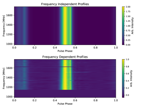
Figure 1: Injected pulse profiles for PSR B1855+09 used for this work. No additional scattering has been injected, and all peaks are normalized to an arbitrary intensity of one. Top: The same pulse profile, here the NANOGrav 11-yr profile for PSR B1955+09, is used for every frequency channel if no frequency-dependent pulse profile evolution is desired. Bottom: Frequency-dependent pulse profiles obtained from modeling a single real observation of PSR B1855+09. No apparent scintillation or spectral index effects remain after following the process detailed in §3.1, and the frequency-dependent variations are clearly shown. Some channels have been removed due to RFI contamination.

Since our frequency-depended profiles were created from real, post-processed observations, profiles at some frequency channels had been removed due to contamination by radio frequency interference (RFI). Since we cannot realistically model profiles in the frequency channels that have been removed, we instead replace them with a profile of zeros. When creating TOAs from these profiles, all channels that were replaced with zeros in this way were removed as well, and are not included in any pulsar timing model fitting (described in §3.2. This 2-D array of frequency-dependent profiles is then input into the psrsigsim as a dataportrait object, and an example is shown in the bottom panel of Figure 1. We note these were all choices made for this work, and that the psrsigsim is capable of using any set of 1- or 2-D user-generated pulse profiles.

While there is some inherent scatter broadening already contained within the real data used for our model frequency-dependent profiles, we do not know a priori how much the profiles have been scatter broadened, and hence can not separate this effect from intrinsic profile evolution. In some of our simulations (described in §4), however, we simulate pulse scatter broadening using the ism class by defining a single input $\tau_{\rm{d}}$, referenced to an initial input frequency, for each simulated epoch. Within the psrsigsim, $\tau_{\rm{d}}$ is scaled for each frequency channel as

$$\tau_{\rm{d}_{i}}=\tau_{\rm{d}}\left(\frac{\nu_{i}}{\nu_{\rm{ref}}}\right)^{\beta}.$$ (2)

Here $\nu_{\rm{ref}}$ is the reference frequency of the input $\tau_{\rm{d}}$, $\nu_{i}$ is the center frequency of the $i$th frequency channel, and $\beta$ is the scaling law exponent. The exponential scattering tail for each frequency channel is then calculated as $\exp(-t/\tau_{\rm{d}_{i}})$, where $t$ is the fractional time of each profile bin. The resulting frequency-dependent exponential scattering tails are then convolved with the pulse profiles. For our simulations, we assume a Kolmogorov medium, so $\beta=-4.4$, though $\beta$ can also be set by the user within the psrsigsim. While it has been found that measurements of $\beta$ deviate from a Kolmogorov medium (e.g. Levin et al., 2016; Turner et al., 2020), we have chosen to use a constant value to minimize the number of variables that affect the covariance between DMX, FD, and $\tau_{\rm{d}}$. While studying how varying $\beta$ may affect these covariances is certainly of interest, this added complexity is beyond the scope of this work.

For this work, we have chosen to run simulations with both a single value of $\tau_{\rm{d}}$ across all epochs and with time-varying $\tau_{\rm{d}}$. In the case of a time-varying $\tau_{\rm{d}}$, we have chosen input values of $\tau_{\rm{d}}$ by randomly sampling a Gaussian distribution with mean and 1$\sigma$ variation reported in Table 1 and then taking the absolute value of the sampled $\tau_{\rm{d}}$. However, for PSR B1953+29, no RMS variation for $\tau_{\rm{d}}$ was reported by Levin et al. (2016), so we use a 1$\sigma$ variation of 20% the mean value. A different value of $\tau_{\rm{d}}$ is then input for every simulated epoch of observations. We note that because the psrsigsim simulates just a single epoch at a time, a user may choose input values for $\tau_{\rm{d}}$ using any method.

After the pulses are simulated, they are dispersed with the ism class. This is done by calculating the time delay due to dispersion,

$$\Delta t_{\rm{DM}}=2.41\times 10^{-4}~{}\mathrm{s}\left(\frac{\rm{DM}}{\rm{pc}~{}\rm{cm}^{-3}}\right)\left(\frac{\nu}{\rm{MHz}}\right)^{-2},$$ (3)

in each frequency channel with respect to infinite frequency. Here $\nu$ is the center frequency of each frequency channel. The pulses are then shifted in Fourier space (Bracewell, 1999) to account for time shifts that are fractional sizes of the discrete time bins. For this work, the DM used is the sum of the base value reported in Table 1 and the individual DMX determined at each epoch as described above. However, we note that in general, the user may input any desired DM into the psrsigsim.

Non-dispersive frequency-dependent time delays are also simulated. In particular, we directly shift the pulses in time to simulate the “FD” model for frequency-dependent pulse profiles. To do this, we calculate $\Delta t_{\rm{FD}}$ as (Zhu et al., 2015; Arzoumanian et al., 2016)

$$\Delta t_{\rm{FD}}=\sum_{i=1}^{n}c_{i}\ln\left({\frac{\nu}{1~{}\rm{GHz}}}\right)^{i}.$$ (4)

Here $c_{i}$ are the polynomial coefficients in time units, more often referred to as the FD parameters, such that $c_{1}=\rm{FD}1$ and so on, $n$ is the number of coefficients, and $\nu$ is the center frequency of each frequency channel. The pulses are then shifted in Fourier space as with $\Delta t_{\rm{DM}}$. Within the psrsigsim the FD parameters are input in units of seconds. We report the number and value of each FD parameter used for each simulated pulsar in this work in Table 1, though in general the user may input any number of FD parameters with any value into the psrsigsim.

Once these delays are added, we then define the telescope used in this work as either the 305-m William E. Gordon Telescope of the Arecibo Observatory or the 100-m Green Bank Telescope of the Green Bank Observatory. We do this using the default arecibo or gbt definition in the psrsigsim, though a user may define any telescope system they wish for their own simulations. Radiometer noise is then added to the simulated data based on the desired receiver-backend configuration. The noise is sampled from a chi-squared distribution with a number of degrees of freedom equal to the number of single pulses in each subintegration. This is then multiplied by the noise variance ($\sigma_{S}$), calculated as defined in Lorimer & Kramer (2012),

$$\sigma_{S}=\frac{\rm{T_{sys}+\rm{T_{sky}}}}{G\sqrt{n_{\rm{p}}~{}dt~{}\rm{BW}_{\rm{chan}}}},$$ (5)

where $\rm{T_{sys}}$ is the system temperature, $\rm{T_{sky}}$ is the sky temperature, $G$ is the telescope gain, $n_{\rm{p}}$ is the number of polarizations, $dt$ is the length of each phase bin or $1/$(sample rate), and $\rm{BW}_{\rm chan}$ is the bandwidth of a frequency channel. Currently the simulator does not model the sky temperature, so we take $\rm{T_{sky}}=0$ for all simulations. Since only total intensity signals are supported at this time, we assume that the total intensity is the sum of two intensities and so $n_{\rm{p}}=2$ for all simulations.

Since the user input profiles are normalized within the psrsigsim, as they may be input with arbitrary units, this is then scaled by the maximum flux, $S_{\rm{max}}$, calculated from the mean flux,

$$S_{\rm{max}}=\frac{S_{\rm{mean}}n_{\rm{bins}}}{\sum_{i=1}^{n_{\rm{bins}}}p_{i}}.$$ (6)

Here $n_{\rm{bins}}$ are the number of phase bins per profile (2048 in all of the simulations in this work), and $p_{i}$ is the intensity of the model profile at the $i$th phase bin. If using frequency-dependent pulse profiles, the profile with the maximum integrated flux (in arbitrary units) is used. This radiometer noise is then further scaled by a normalization coefficient, $U_{\rm{scale}}$, since, as mentioned above, the model profiles are normalized within the pulsar class. This constant is calculated as defined in Lam (2018),

$$U_{\rm{scale}}=\frac{1.0}{\left(\sum_{i=1}^{n_{\rm{bins}}}p_{i}\right)/n_{\rm{bins}}},$$ (7)

where again the profile used is from the frequency channel that results in the maximum integrated flux.

The final simulated data are contained within a numpy array (Van Der Walt et al., 2011). However, for this work, since we require the use of the psrchive software, we have used the convenience functions provided in the io class and described in §2 to save the full simulated data array as a psrfits file (Hotan et al., 2004) as described in §2.

3.2 TOAs and Residuals

Once the data have been simulated in psrfits file format, they are analyzed with both psrchive and pint . The data are simulated such that all observations match the post-processed NANOGrav standard timing methods (Demorest, 2018), with a single subintegration and 64 frequency channels. For simulated Arecibo data, this results in frequency channels with widths of 1.5625 and 12.5 MHz at 430 and 1400 MHz, respectively. For simulated GBT data, this results in frequency channels with widths of 3.125 and 12.5 MHz at 820 and 1400 MHz, respectively.

TOAs are obtained from the simulated data with the pat function in psrchive. We use the corresponding NANOGrav 11-yr pulse profile templates for the template matching process. This method employs a constant template profile at the appropriate frequency bands regardless of whether frequency-dependent profiles were used in the simulations to better match the standard template-fitting methods used by NANOGrav (Taylor, 1992; Demorest, 2018).

Normally, certain frequency channels are ignored in the NANOGrav timing pipeline as they are highly contaminated by RFI (Arzoumanian et al., 2016; Demorest, 2018). While we generate no RFI in our simulated data, we mimic this loss in sensitivity by removing all TOAs from these ranges in all simulation analyses. This includes channels where no frequency-dependent profile model has been generated, as described above and shown in Figure 1. For simulated Arecibo data, the removed ranges are 380–423, 442–480, 980–1150, and 1618–1630 MHz. For simulated GBT data, the removed ranges are 794.6–798.6, 814.1–820.7, 1100–1150, 1250–1262, 1288–1300, 1370–1385, 1442–1447, 1525–1558, 1575–1577, 1615–1630 MHz.

We then calculate the timing residuals using the pint pulsar timing package (Luo et al., 2020). Each pulsar timing model is extremely simple and includes only the position, period, DM, DMX, the number of FD parameters equal to that listed in Arzoumanian et al. (2018a), and one JUMP parameter to account for unmodeled profile evolution and other effects between the low and high frequency simulated data. Of these we fit only combinations of DMX, FD, and JUMP parameters, holding all other values fixed. Since we have not included any motions of the Earth, we assume that all TOAs that we have obtained are already barycentered. We do not include any effects such as parallax, proper motion, or binary motion and therefore do not fit for these in our timing model.

When fitting the different DMX values for each simulation, we follow Arzoumanian et al. (2016) and Arzoumanian et al. (2018a) and bin our simulated TOAs in groups of 15 days for simulated epochs before MJD 56000, and 6 days after MJD 56000. The adjustment in binning comes from the less frequent observations that occurred early on in the NANOGrav timing program (Arzoumanian et al., 2018a). We then fit our timing model parameters using the generalized least squares fitter in pint and compare the fit values of DMX and the FD parameters, which we will denote as $\widehat{\rm{DMX}}$ and $\widehat{\rm{FD}}$, to the injected values.

4 Simulated Data

The parameters that were used to make the simulated data for PSRs J1744–1134, B1855+09, and B1953+29 are shown in Table 1. We note that while real pulsars have many additional timing parameters (e.g., spin down, proper motions, etc.), we do not simulate these effects in any of our data sets presented here. Our simulated data therefore represent barycentered observations that have had all non-frequency-dependent delays removed.

Table 1: Simulated Pulsar Parameters

Parameter	J1744$-$1134	B1855+09	B1953+29
Period (ms)	4.075	5.362	6.133
DM (pc cm-3)	3.09	13.30	104.5
FD1 ($\upmu$s)	$-383.4\pm 88.5$	$128.7\pm 24$	$139.5\pm 7.8$
FD2 ($\upmu$s)	$395.6\pm 89.5$	$-147.5\pm 29$	$-61.0\pm 7.8$
FD3 ($\upmu$s)	$-241.1\pm 60.2$	$81.6\pm 18$	-
FD4 ($\upmu$s)	$98.9\pm 23.3$	-	-
$S_{430}$ (mJy)	-	14.56	10.77
$S_{820}$ (mJy)	2.93	-	-
$S_{1400}$ (mJy)	0.98	2.13	0.69
$\alpha$	$-1.77$	$-1.45$	$-2.16$
$\tau_{\rm{d}}$ (ns)	$3.3\pm 1.6$	$8.1\pm 4.4$	$55.3(\pm 11.1)$

Scattering timescales $\tau_{\rm{d}}$ are all referenced to 1500 MHz and for PSRs J1744$-$1134 and B1855+09 come from Turner et al. (2020), and for PSR B1953+29 from Levin et al. (2016). All uncertainties are $1\sigma$, with the uncertainties on scattering delay defined as the RMS variation over the data set. No variation on $\tau_{\rm{d}}$ for PSR B1953+29 was reported in Levin et al. (2016) so we define it to be 20% the measured value.

Note. — Parameters describing the three MSPs that were used in these simulations. Period, DM, and FD1-4 values are from the NANOGrav 11-yr data set (Arzoumanian et al., 2018a). Flux values ($S$) and spectral index ($\alpha$) values are from Alam et al. (2020a).

The simulated data sets for each pulsar are split into two sets of simulations. The first set consists of simulations where the pulse profile is frequency-independent for a given observing band. The recovered parameters generally match the injected parameters in this set and are used primarily for comparison. The second set uses realistic, frequency-dependent pulse profiles as described in §3.1. In total, we simulated nine different data sets with different injections for each pulsar. Five of them used frequency-independent pulse profiles for comparison purposes, and the other four were used to analyze the covariances between the frequency-dependent parameters. The basic injections and values used for each simulation can be found in Table 4.

All simulations span the same length as the observations of each pulsar using the NANOGrav observing epochs from Arzoumanian et al. (2018a). While it is not necessary to simulate a full data set like this to explore the covariances between these parameters, we do this in part to demonstrate that the psrsigsim can simulate long sets of unevenly samples observing epochs while maintaining a precise phase connection. In addition, it demonstrates the efficiency of the psrsigsim, as the total time for each of the nine simulations to run for the two longer data sets, those of PSRs J1744–1134 and B1855+09, was $\sim 5$ minutes on an Intel(R) Xeon(R) CPU E5-2630 0 @ 2.30GHz with 24 processors and 64 GB of RAM. In addition to using realistic observing epochs as a benchmarking test for the psrsigsim, having many DMX bins better quantifies the variations that may be seen in DMX due to profile evolution or scatter broadening. Finally, as the FD parameters are fit globally over the entire data set, their fit values are sensitive to the length and number of observations in the simulated data set.

For simulated observations using the Arecibo telescope, we simulate only data from the PUPPI backend (Ford et al., 2010) and for observations simulated using the GBT, we simulate only data using the GUPPI backend (DuPlain et al., 2008). While much of the early observations of these MSPs were done with the GASP or ASP backend (Demorest, 2007), there are additional systematics introduced into the pulsar timing when switching between backends that is beyond the scope of this work. The observing frequencies of each pulsar, either 430 MHz or 1400 MHz at Arecibo or 820 MHz or 1400 MHz at the GBT, are the same as in Arzoumanian et al. (2018a). The parameters for each receiver-backend combination are reported in Table 2. The observation lengths, the time of each simulated observing epoch, come from the length of the actual observation that was used to generate the frequency-dependent pulse profiles. These lengths represent a typical observing length for each pulsar as observed by NANOGrav, though they are kept constant for each simulated observing epoch.

Table 2: Description of Backend/Receiver Parameters

PSR	Backend	Receiver	MJD Range	Center Frequency	Bandwidth	Frequency Channels	Observation Length
				(MHz)	(MHz)		(s)
J1744$-$1134	GUPPI	820	53217-57369	820	200	64	1578
J1744$-$1134	GUPPI	L-wide	53216-57367	1500	800	64	1742
B1855+09	PUPPI	430	53358-57375	430	100	64	1204
B1855+09	PUPPI	L-wide	53358-57375	1380	800	64	1270
B1953+29	PUPPI	430	55760-57348	430	100	64	1443
B1953+29	PUPPI	L-wide	55760-57376	1380	800	64	1440

Note. — Parameters used for each simulated backend. MJD ranges, center frequencies, bandwidths, taken from the NANOGrav 11-yr data set (Arzoumanian et al., 2018a). All simulated observations were simulated with 64 frequency channels. Observation lengths are from the observations which were used to obtain high S/N pulse profile templates.

Table 3: DM Variation Parameters

PSR	DM Slope	DM Amplitude	DM Period
	($10^{-3}$ pc cm-3 yr-1)	($10^{-4}$ pc cm-3)	(days)
J1744$-$1134	$-0.069$	0.4	383
B1855+09	0.382	0.5	364
B1953+29	$-1.3$	3.0	356

Note. — Slope, amplitude, and period of the DM variations used for each pulsar that was simulated as derived by Jones et al. (2017).

Table 4: Description of Simulated Data sets

Simulation Name	DM Variations	FD Injection	Profile Evolution	Constant Scatter Broadening	Time-Variable Scatter Broadening
No Variations	N	N	N	N	N
DM Variations	Y	N	N	N	N
FD Injections	N	Y	N	N	N
Time-Variable Scatter Broadening w/ Constant DM	N	N	N	N	Y
DM & FD Injections	Y	Y	N	N	N
Profile Evolution	N	N	Y	N	N
DM & Profile Evolution	Y	N	Y	N	N
Scatter Broadening	Y	N	Y	Y	N
Time-Variable Scatter Broadening	Y	N	Y	N	Y

Note. — Description of parameters included in each simulated data set. A ‘Y’ means the parameter was injected into the simulation, while ‘N’ means it was not injected. If DM variations are included, the slope, amplitude, and period of the DM variations are presented in Table 3. If FD injection is included the profiles used do not vary in frequency and are instead direction shifted in time by the delay described the NANOGrav 11-yr FD parameters. If profile evolution is used, then frequency-dependent profile models based on actual observations of each pulsar are used for the injected pulse profiles. If scatter broadening is used, then the injected profiles are convolved with an exponential described by a scattering timescale, $\tau_{\rm{d}}$. If constant, then each epoch uses the mean value of $\tau_{\rm{d}}$ from Table 1, if time-variable, $\tau_{\rm{d}}$ is drawn from a Gaussian distribution with a mean and standard deviation from Table 1.

4.1 Frequency-Independent Pulse Profile Simulations

The first simulation in this set was the “No Variation” simulation. Every simulated epoch used a constant value of DM (e.g., all DMX values were zero), and included no additional time delays (e.g., from FD parameters or scatter broadening). The purpose of this was to test the simplest case simulation and provide a baseline to compare to other simulations with addition injected effects. For each observation we determine $\Delta\rm{DM}$, the recovered DMX minus the injected DMX, $\Delta\rm{DM}=\widehat{\rm{DMX}}-\rm{DMX}$. This is shown in red at every simulated observing epoch for all three simulated pulsars in Figure 2. We note that the $\widehat{\rm{DMX}}$ values have been mean subtracted as $(\widehat{\rm{DMX}}_{i}-\langle\widehat{\rm{DMX}}\rangle)$ for each DMX epoch $i$, and the error bars shown represent the errors on the mean subtracted value. This is done because it allows us to separate the uncertainty of each DMX measurement from that of the mean DM, since there is a large covariance between these parameters (Arzoumanian et al., 2016, 2018a).

We similarly determine $\Delta\rm{FD}$ parameters, the recovered FD parameter minus injected FD parameter, $\Delta{\rm{FD}}_{\rm{i}}=\widehat{\rm{FD}_{\rm{i}}}-{\rm{FD}}_{i}$, for each individual FD parameter i. For this simulation, these shown in red in the two upper panels of Figures 3, 4, and 5 for each pulsar respectively. All of the recovered $\Delta\rm{DM}$ and $\Delta\rm{FD}$ parameters for these simulations are shown in the same panels of the same Figures, though with different colors. All recovered values, $\widehat{\rm{DMX}}$ and $\widehat{\rm{FD}}$, shown in these figures were determined by fitting for all parameters: DMX, all FD parameters, and a single JUMP parameter.

The second simulation is the “DM Variations” simulation. Here the total injected DM is the initial value given in Table 1 plus a small variation added based on the parameters given in Table 3. The variations for all simulated pulsars had both a linear and sinusoidal trend with slope, amplitude, and period as determined by Jones et al. (2017). The resulting $\Delta\rm{DM}$ and $\Delta\rm{FD}$ parameters, similar to that shown for the “No Variations” simulation, are shown in purple.

The third simulation in this set is the “FD Injection.” While the physical process that FD parameters describe is mainly attributed to pulse profile evolution in frequency (Zhu et al., 2015), they define a time delay directly given by Eq. 4. To provide a baseline for recovering the injected FD parameters, we directly shift the simulated pulses in time based on the FD parameters listed in Table 1. We do this instead of varying the profiles directly because we do not know a priori what the shifts due to profile evolution are, we can only fit them empirically. The resulting $\Delta\rm{DM}$ and $\Delta\rm{FD}$ parameters for this simulation are shown in orange.

The fourth simulation here is “Time-Variable Scattering with Constant DM.” Here we again use a constant value of DM, but also inject time-variable values of $\tau_{\rm{d}}$ on a per-epoch basis, selected as described in §3.1. This gives us baseline to compare how $\widehat{\rm{DMX}}$ is affected by this time-variable scattering in more complex simulations. The resulting $\Delta\rm{DM}$ and $\Delta\rm{FD}$ parameters for this simulation are shown in light green.

Our final initial simulation, “DM & FD Injections” is a combination of the second and third initial simulations. This was done to provide a baseline for the accuracy of $\widehat{\rm{DMX}}$ and $\widehat{\rm{FD}}$ since they are both dependent on the emission frequency. The resulting $\Delta\rm{DM}$ and $\Delta\rm{FD}$ parameters for this simulation are shown in light blue.

While all of the recovered values shown in Figures 2, 3, 4, and 5 come from fitting for all parameters, DMX, all FD parameters, and a JUMP, we also fit each of these simulations using just a single JUMP, just DMX and a single JUMP, and just all applicable FD parameters and a single JUMP (for a total of four different fits for each simulation). We report the RMS of the timing residuals ($\cal{R}_{\rm{rms}}$), reduced chi-squared ($\chi^{2}_{\rm{r}}$ of the fit timing model, the RMS of the $\Delta\rm{DM}$ values ($\widehat{\rm{DMX}}-\rm{DMX}$), $\Delta\rm{DM}_{\rm{rms}}$, the RMS of the $\Delta\rm{FD}$ parameters ($\widehat{\rm{FD}_{\rm{i}}}-\rm{FD}_{i}$), $\Delta\rm{FD}_{\rm{rms}}$, and the fit value of the JUMP, for each of these fits per simulation per pulsar in Tables 5, 6, and 7 respectively.

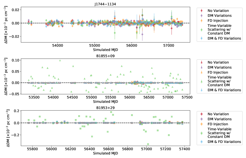
Figure 2: Resulting $\Delta\rm{DM}$ values for all three simulated pulsars for simulations where no frequency-dependent pulse profiles were used (described in §4.1) when fitting for DMX, all FD parameters, and a JUMP. Different symbols are used for each pulsar. The black dashed lines represent the zero lines. All points for each pulsar and each simulation are scattered around this zero line, showing that they are being appropriately recovered and fit for.

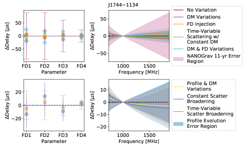
Figure 3: Upper Left: Resulting $\Delta\rm{FD}$ parameters for five different simulated data sets of eleven years where no frequency-dependent pulse profiles were used for PSR J1744–1134 (described in §4.1). All recovered values come from fitting for DMX, all FD parameters, and a JUMP. The recovered parameters match well with the injected parameters. Upper Right: Same as upper left but showing the delay curve across frequency space defined by the $\Delta\rm{FD}$ parameters shown in the upper left plot. Shaded regions represent the 1$\sigma$ recovered errors. Lower Left: Same as upper left, but for four different simulations where frequency-dependent pulse profiles were used (described in §4.2). Lower Right: Same as upper right, but for the simulations listed in the lower left.

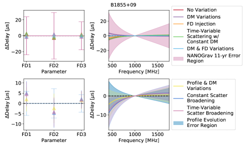
Figure 4: Upper Left: Resulting $\Delta\rm{FD}$ parameters for five different simulated data sets of eleven years where no frequency-dependent pulse profiles were used for PSR B1855+09 (described in §4.1). All recovered values come from fitting for DMX, all FD parameters, and a JUMP. The recovered parameters match well with the injected parameters. Upper Right: Same as upper left but showing the delay curve across frequency space defined by the $\Delta\rm{FD}$ parameters shown in the upper left plot. Shaded regions represent the 1$\sigma$ recovered errors. Lower Left: Same as upper left, but for four different simulations where frequency-dependent pulse profiles were used (described in §4.2). Lower Right: Same as upper right, but for the simulations listed in the lower left.

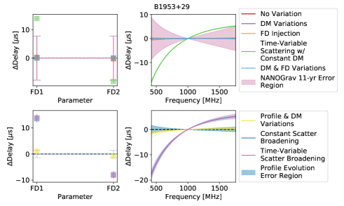
Figure 5: Upper Left: Resulting $\Delta\rm{FD}$ parameters for five different simulated data sets of eleven years where no frequency-dependent pulse profiles were used for PSR B1953+29 (described in §4.1). All recovered values come from fitting for DMX, all FD parameters, and a JUMP. The recovered parameters match well with the injected parameters. Upper Right: Same as upper left but showing the delay curve across frequency space defined by the $\Delta\rm{FD}$ parameters shown in the upper left plot. Shaded regions represent the 1$\sigma$ recovered errors. Lower Left: Same as upper left, but for four different simulations where frequency-dependent pulse profiles were used (described in §4.2). Lower Right: Same as upper right, but for the simulations listed in the lower left.

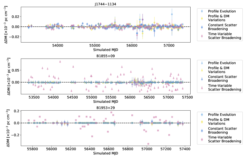
Figure 6: Resulting $\Delta\rm{DM}$ values for all three simulated pulsars for simulations where frequency-dependent profile evolution was modeled (described in §4.2) when fitting for DMX, all FD parameters, and a JUMP. Different symbols are used for each pulsar. The black dashed lines represent the zero lines. All points for each pulsar and each simulation are scattered around this zero line, showing that they are being appropriately recovered and fit for.

4.2 Frequency-Dependent Pulse Profile Simulations

Next we use a different set of frequency-dependent profiles, one for each different receiver-backend combination for each pulsar, is used as described in §3. As noted in §3.1, we use only one set of frequency-dependent profiles for each receiver-backend combination. Since there are no variations in the profile evolution in time, e.g., due to scintillation (Cordes, 1986), we do not expect to recover exactly the same FD parameters as reported in Table 1. We do, however, expect similar FD parameters, with the same signs and orders of magnitude.

To determine what the contribution of the frequency-dependent profiles is to the FD parameters, our first simulation in this set, labeled “Profile Evolution”, uses a constant DM such that all injected DMX values are zero, and includes only the frequency-dependent profile. This allows us to determine what the expected contribution of the chosen set of frequency-dependent profiles is, and help to quantify any deviations in $\widehat{\rm{FD}}$ as more frequency-dependent effects are added. The resulting $\Delta\rm{DM}$, similar to that shown for the previous set of simulations, are shown in blue in Figure 6 and the resulting $\Delta\rm{FD}$ parameters for this simulation, also in blue, are shown in the two lower panels of Figures 3, 4, and 5 for each pulsar respectively. All values of $\Delta\rm{DM}$ and $\Delta\rm{FD}$ parameters for these simulations are shown in the same panels of the same Figures, though with different colors. The resulting $\Delta\rm{FD}$ parameters for this simulation have values of zero with an associated error bar, since we do not know their value a priori. For this simulation $\widehat{\rm{FD}}$ are used as the baseline for all other simulations in this set.

The second simulation, “DM & Profile Evolution”, uses both the frequency-dependent profiles as well as the DM variations that were used in the initial simulations described in §4.1. This simulation allows us to explore the covariances between DMX and profile evolution, and compare them to the covariances when FD parameters are directly injected via time shift. The resulting $\Delta\rm{DM}$ and $\Delta\rm{FD}$ parameters for this simulation are shown in yellow.

The third simulation, “Scatter Broadening,” is the same as “DM & Profile Evolution” but here the frequency-dependent profiles have been convolved with an exponential defined by a single mean scattering time scale, given in Table 1. As pulse scatter broadening is also a frequency-dependent effect, we expect it to have some small effect on $\widehat{\rm{DMX}}$ and $\widehat{\rm{FD}}$ (Rickett, 1977; Levin et al., 2016). However, since for this simulation only a constant value of $\tau_{\rm{d}}$ is injected, we expect the FD parameters to account for most, if not all of this variation (Zhu et al., 2015; Arzoumanian et al., 2016). The resulting $\Delta\rm{DM}$ and $\Delta\rm{FD}$ parameters for this simulation are shown in dark blue.

The final simulation of this set, “Time-Variable Scatter Broadening”, is the same as “Scatter Broadening” but here we have randomly sampled values of $\tau_{\rm{d}}$ to be injected at each epoch as described in §3.1. This simulation represents the most realistic of our simulations. Since here $\tau_{\rm{d}}$ changes, we expect $\widehat{\rm{DMX}}$ to be effected more substantially as the FD parameters are fit over the entire data set, not epoch to epoch. The resulting $\Delta\rm{DM}$ and $\Delta\rm{FD}$ parameters for this simulation are shown in magenta.

As with the previous set of simulations, all of the values shown in Figures 3, 4, 5, and 6 come from fitting for all parameters: DMX, all FD parameters, and a JUMP. We report $\cal{R}_{\rm{rms}}$, $\chi^{2}_{\rm{r}}$, $\Delta\rm{DM}_{\rm{rms}}$, $\Delta\rm{FD}_{\rm{rms}}$, and the fit value of the JUMP for this set of fit model parameters, as well as the additional model fitting done with a single JUMP, just DMX and a single JUMP, and just all FD parameters and a single JUMP, in Tables 5, 6, and 7. We note that for this set of simulations, when computing $\Delta\rm{FD}_{\rm{rms}}$, two different sets of FD parameters were used, one set that was fit for using DMX, FD, and a JUMP, and one where just FD and a JUMP was used, both sets come from the “Profile Evolution” simulation. This is because the FD parameters are covariant with DMX and the values change slightly depending on what parameters are fit for.

5 Results

Here we describe the results of the simulations described in §4 for each pulsar. Figures 2, 3, 4, 5, and 6 show the results of simulation analyses when we fit for all parameters (DMX, all FD parameters, and a JUMP). Figures 2 and 6 shows the $\Delta\rm{DM}$ (the difference between the injected and recovered DM, $\widehat{\rm{DMX}}-\rm{DMX}$) for each simulated epoch for all MSPs. Each set of simulations is split into two sets, Figure 2 shows the simulations described in §4.1 Figure 6 shows the $\Delta\rm{DM}$ for the simulations described in §4.2. In these Figures, we again note that the $\Delta\rm{DM}$ values have been mean subtracted as described in §4.1, so we expect all points to be scattered around a mean of zero. This allows for better visualization of the spread in $\Delta\rm{DM}$ between different simulations, where a tighter spread indicates more precise recovery of the injected values. We also note that there are a few $\Delta\rm{DM}$ values that have particularly large error bars. This is an artifact of the $\widehat{\rm{DMX}}$ bin sizes. Points with these larger uncertainties only have higher frequency 1400 MHz simulated observations within the fifteen or six day window leading to a less accurate $\widehat{\rm{DMX}}$.

Figures 3, 4, and 5 show the $\Delta\rm{FD}$ parameters (the difference between the injected and recovered FD parameters, $\widehat{\rm{FD}_{\rm{i}}}-\rm{FD}_{i}$) for for all simulated MSPs, with the top and bottom sets of panels broken up by simulation. The left hand plots in these Figures show $\Delta\rm{FD}$ for each individual FD parameter in each MSP. The right hand plots show the total time delay described by the $\Delta\rm{FD}$ parameters calculated using Eq. 4, as a function of radio frequency. For all simulations without scatter broadening, when we fit for all parameters, the resulting $\Delta\rm{FD}$ parameters are distributed around zero, and within $1\sigma$ of the injected values as shown in Figures 2, 3, 4, 5, and 6.

We also compare how fitting for different combinations of DMX, FD parameters, and a JUMP affect both the timing residuals, quantified by $\cal{R}_{\rm{rms}}$, and the timing model, quantified by $\chi^{2}_{\rm{r}}$, as reported in Tables 5, 6, and 7. These tables also list the values of $\Delta\rm{DM}_{\rm{rms}}$ and $\Delta\rm{FD}_{\rm{rms}}$, which are used to determine how precisely $\widehat{\rm{DMX}}$ and $\widehat{\rm{FD}}$ are recovered. A large value means that the parameters are recovered less precisely, while smaller values indicate a more precise recovery.

As expected, we see that fitting for additional parameters, e.g., adding FD parameters even when none have been injected into the simulation, does not negatively impact the $\cal{R}_{\rm{rms}}$ for any simulated data sets. The $\chi^{2}_{\rm{r}}$ for each fit also appear to be generally unaffected by the addition of more model parameters, however this is due to both the slightly decreased $\chi^{2}$ value of these fits, and the reporting of $\chi^{2}_{\rm{r}}$ to only two decimal places. Further, when adding additional parameters to the simulations, e.g., DM variations or FD parameters, the recovered $\cal{R}_{\rm{rms}}$ when all injected parameters are fit for agree as expected, confirming our methods.

5.1 Discussion of Frequency-Independent Profile Simulations

As FD parameters primarily model variations in the pulse profile with observing frequency (Zhu et al., 2015; Arzoumanian et al., 2016), we expect that $\widehat{\rm{FD}}$ should all be consistent with zero, and $\Delta\rm{FD}_{\rm{rms}}$ should be very small for these simulations . The exception would be if the profiles are directly shifted in time, or altered in some way (e.g., scatter broadening) as a function of frequency, as denoted in Table 4. The injected spectral index does not alter the shape or the profiles, and should not cause additional variations in the FD parameters. This is indeed what we find, as shown by the upper right panels of Figures 3, 4, 5.

In the “No Variations” simulations, we find that regardless of what combination of parameters are fit for, we recover almost the same $\cal{R}_{\rm{rms}}$. This shows that adding additional parameters does not negatively impact the precision of our pulsar timing and confirms that they are not absorbing any additional non-frequency-dependent (or white) noise in the simulated data.

For the “Time-Variable Scatter Broadening w/ Constant DM ”, we find that for all simulated pulsars, the $\cal{R}_{\rm{rms}}$ and $\chi^{2}_{\rm{r}}$ are slightly larger than for the “No Variation” simulation. The effect of the scattering delays are obvious from the light green points in Figure 2, where the larger the average value, and hence spread of, $\tau_{\rm{d}}$, the less accurate and more variable the resulting $\Delta\rm{DM}$, and subsequently $\widehat{\rm{DMX}}$, is. This is less obvious in Figure 3, but in Figures 4 and 5, the inability to recover accurate FD parameters due to larger average injected $\tau_{\rm{d}}$ values is apparent as the light green curve is not consistent with zero. This indicates that the DMX and FD parameters cannot appropriately account for time-variable scattering delays, though the larger variation in the $\Delta\rm{DM}$ values suggest that the additional delays from scattering are absorbed by $\widehat{\rm{DMX}}$, showing a clear covariance between these two frequency-dependent effects.

For all other simulations in this set, the resulting $\cal{R}_{\rm{rms}}$ and $\chi^{2}_{\rm{r}}$ show that when the appropriate parameters are fit for, all frequency-dependent delays are accounted for, affirming our expectations. When only FD parameters are injected and all parameters are fit for, $\Delta\rm{FD}_{\rm{rms}}$ increases and $\Delta\rm{DM}_{\rm{rms}}$ either remains constant or decreases. This is indicative of a small covariance between DMX and the FD parameters, and shows that FD parameters are more susceptible to variations than DMX is when additional frequency-dependent effects are present and fit. While this is expected (Zhu et al., 2015), it increases our confidence that when there is very little or no scattering, the FD parameters are absorbing very little of the dispersive delays. In these cases, such as PSR J1744–1134, we can be reasonably confident that the injected DM is being recovered.

In real pulsar timing data, both DM variations and additional non-$\nu^{-2}$ frequency-dependent effects are present. The results of this set of simulations shows that we can accurately recover the full injected delay, when the scattering timescale is very small or zero, giving us confidence in both our methods, and our ability to use this set of simulations as a comparison to our more complex simulations.

5.2 Discussion of Frequency-Dependent Profile Simulations

In the “Profile Evolution” simulations, $\chi^{2}_{\rm{r}}$ is consistent when fitting for just FD parameters and all parameters, for PSRs J1744–1134 and B1855+09. However, for PSR B1953+29, $\chi^{2}_{\rm{r}}$ is lower when fitting for all parameters compared to just FD parameters. As PSR B1953+29 has a much higher DM, this suggests that $\widehat{\rm{DMX}}$ may absorb more of the delays from profile evolution at higher DMs. It is possible that this is because at higher DMs, the profile evolution may be primarily dominated by scattering. Since scattering scales in a similarly frequency-dependent way to DM, $\widehat{\rm{DMX}}$ may absorb the effects of scatter broadening more at higher DMs. We note, however, that as we have simulated only three MSPs it is difficult to verify this. To fully explore this relationship would require additional simulations of comparable length exploring not only the scale of DM, but also the size of the DM variations and the number of FD parameters, and as such is beyond the scope of this work. Additionally, since we recover very similar values of $\cal{R}_{\rm{rms}}$ and $\chi^{2}_{\rm{r}}$ for all MSPs using both methods of fitting, $\widehat{\rm{DMX}}$ likely fits out very little of this intrinsic profile evolution, which is expected (Zhu et al., 2015; Arzoumanian et al., 2016).

In all other simulations in this set, we find that the best values of $\cal{R}_{\rm{rms}}$ and $\chi^{2}_{\rm{r}}$ occur when we fit for all parameters, which is consistent with the previous simulations discussed in §5.1. For the “Time-Variable Scatter Broadening” simulation, we note that $\cal{R}_{\rm{rms}}$ is comparable to those obtained in the other simulations in this set, despite Figure 6 showing that when the average $\tau_{\rm{d}}$ is large, $\widehat{\rm{DMX}}$ is much less accurate and more variable. This is consistent with the results from the “Time-Variable Scatter Broadening w/ Constant DM ” and suggests that the average scatter broadening is completely fit out by the FD parameters, while the time variations in the injected $\tau_{\rm{d}}$ are primarily absorbed by the DMX parameters. This again shows the clear covariance between DM and scattering.

For PSR J1744–1134, which has both the lowest DM and the most FD parameters of our simulated pulsars, we find that $\Delta\rm{FD}_{\rm{rms}}$ decreases while $\Delta\rm{DM}_{\rm{rms}}$ stays comparable when going from a constant to time-varying injected $\tau_{\rm{d}}$. This is in contrast to both PSRs B1855+09 and B1953+29, which show an increase in $\Delta\rm{DM}_{\rm{rms}}$ but a roughly constant $\Delta\rm{FD}_{\rm{rms}}$ when $\tau_{\rm{d}}$ varies with time. It is difficult to determine if this suggests that pulsars with more FD parameters and/or smaller $\tau_{\rm{d}}$ are less effected by time-varying $\tau_{\rm{d}}$, or if this is an artifact of pulsars we have chosen to simulate. In all simulations in this set for PSR J1744–1134 $\Delta\rm{FD}_{\rm{rms}}$ is larger when fitting for all parameters than just FD parameters, which may similarly suggest that the covariance between DMX and the FD parameters is larger for more FD parameters and/or smaller DM or DM variations. In either case, a comprehensive analysis of this potential relationship would involve exploring a large parameter space, mentioned above, that is beyond the scope of this work.

The difference between the constant and time-varying scatter broadening simulations most clearly shows that while there may be a covariance between DMX and FD parameters, it is very small. As the FD parameters are fit over the full data set, the differences in $\Delta\rm{FD}_{\rm{rms}}$ from a constant to time-varying $\tau_{\rm{d}}$ are much smaller than those of $\Delta\rm{DM}_{\rm{rms}}$. Since the DMX are fit as a piece-wise function over small timescales, they account for most of the additional time-varying scattering delays. While this means $\widehat{\rm{DMX}}$ may not be as accurate, we can see that it does not seem to have a large effect on $\cal{R}_{\rm{rms}}$, since for both scattering simulations in this set this value is comparable to the smallest $\cal{R}_{\rm{rms}}$ in the baseline “Profile Evolution” simulation.

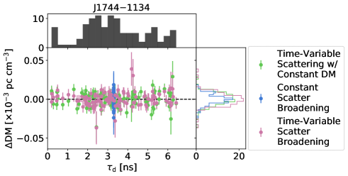
Figure 7: $\Delta\rm{DM}$ value ($\widehat{\rm{DMX}}-\rm{DMX})$ versus the injected scattering timescale(s) $\tau_{\rm{d}}$ within each DMX bin for PSR J1744–1134. There are the same number of points for each simulation shown. We can see that in the case of time-variable scattering delays, the injected DMX value is recovered less accurately shown by the larger spread in the green and magenta $\Delta\rm{DM}$ points compared to the blue points. The top histogram shows the distribution of injected $\tau_{\rm{d}}$ while the right histogram shows the distribution of $\Delta\rm{DM}$. We clearly see no correlation between the injected value $\tau_{\rm{d}}$ and the $\Delta\rm{DM}$, showing that time-variable scattering only serves to make $\widehat{\rm{DMX}}$ more variable and less accurate, though minimally for small average values of $\tau_{\rm{d}}$.

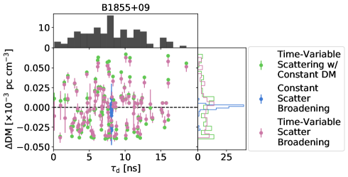
Figure 8: $\Delta\rm{DM}$ value ($\widehat{\rm{DMX}}-\rm{DMX}$) versus the injected scattering timescale(s) $\tau_{\rm{d}}$ within each DMX bin for PSR B1855+09. There are the same number of points for each simulation shown. We can see that in the case of time-variable scattering delays, the injected DMX value is recovered less accurately, as shown by the larger spread in the green and magenta $\Delta\rm{DM}$ points compared to the blue points. The top histogram shows the distribution of injected $\tau_{\rm{d}}$ while the right histogram shows the distribution of $\Delta\rm{DM}$. We clearly see no correlation between the injected value $\tau_{\rm{d}}$ and the $\Delta\rm{DM}$, showing that time-variable scattering only serves to make $\widehat{\rm{DMX}}$ more variable and less accurate.

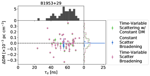
Figure 9: $\Delta\rm{DM}$ value ($\widehat{\rm{DMX}}-\rm{DMX}$) versus the injected scattering timescale(s) $\tau_{\rm{d}}$ within each DMX bin for PSR B1953+29. There are the same number of points for each simulation shown. We can see that in the case of time-variable scattering delays, the injected DMX value is recovered less accurately shown by the larger spread in the green and magenta $\Delta\rm{DM}$ points compared to the blue points. The top histogram shows the distribution of injected $\tau_{\rm{d}}$ while the right histogram shows the distribution of $\Delta\rm{DM}$. We clearly see no correlation between the injected value $\tau_{\rm{d}}$ and the $\Delta\rm{DM}$, showing that time-variable scattering only serves to make $\widehat{\rm{DMX}}$ more variable and less accurate.

6 Implications for Precision Pulsar Timing

The results of our simulations and analyses are important when considering the use of PTAs to detect gravitational waves (e.g., McLaughlin, 2013; Kramer & Champion, 2013; Hobbs, 2013). In all simulated MSPs, we find that when profile evolution is present through direct injection or the use of frequency-dependent profiles, $\Delta\rm{FD}_{\rm{rms}}$ can change by an order of magnitude when all parameters are fit for, compared to just FD parameters. In general this change seems to be an increase for pulsars with more FD parameters and smaller DMs, and a decrease for pulsars with larger DMs and fewer FD parameters, however it is important to note that we have only simulated three pulsars in this work. Regardless, this is evidence of the covariance between DMX and FD parameters especially in the simulations where no scattering delays are injected, however the effect on $\cal{R}_{\rm{rms}}$ in negligible, as it is always at a minimum when all appropriate parameters have been fit for. Additionally, $\chi^{2}_{\rm{r}}$ is almost always closest to one when fitting for all parameters, showing that the addition of FD parameters does not make the timing model fit worse.

Additionally, one can see from Figures 2 and 6 that, when no time-variable scattering delays are injected, as long as the DMX fit spans both frequency bands, we can recover the injected DMX, regardless of the DM variations, the nominal DM value, or the number of FD parameters. This shows that, as expected (Zhu et al., 2015; Arzoumanian et al., 2016), our models and fitting are able to, in principle, separate out the physical variations in DM from any effects modeled out by FD parameters. We can conclude that though there is a definitive covariance between DMX and the FD parameters, it is very small, and does not affect the precision of the pulsar timing.

The most interesting result and impact found in our simulations is when time-variable $\tau_{\rm{d}}$ are injected. It is apparent from Figures 2, 3, 4, 5, and 6 that these time-variable delays decrease the accuracy and increase the variability of $\widehat{\rm{DMX}}$ as well as $\widehat{\rm{FD}}$, and that the level of inaccuracy and variability increases with larger values of $\tau_{\rm{d}}$. This seems to indicate that the time delays due to scattering are primarily absorbed by the DMX values indicating a clear covariance between the two frequency-dependent effects. This shows that in real pulsar data, larger scattering timescales will result in some of the variations in $\widehat{\rm{DMX}}$. However, in our most realistic simulation, “Time-Variable Scatter Broadening”, $\cal{R}_{\rm{rms}}$ is within 10 ns of the minimum expected $\cal{R}_{\rm{rms}}$ given in our baseline “Profile Evolution” simulation. So even though the time-variable scattering clearly changes the $\widehat{\rm{DMX}}$ and $\widehat{\rm{FD}}$, it has a minimal effect on $\cal{R}_{\rm{rms}}$, at least for the three pulsars simulated in this work.

Since $\widehat{\rm{DMX}}$ have a much larger spread with varying $\tau_{\rm{d}}$, we also look to see if there is a correlation between the two parameters. The $\Delta\rm{DM}$ values are plotted against the values of $\tau_{\rm{d}}$ injected within each DMX epoch in Figures 7, 8, and 9. In all cases, we can see that for simulations with time-variable scattering delays (green and magenta), the larger the average value, and hence spread of, $\tau_{\rm{d}}$, the larger the spread in $\Delta\rm{DM}$. For simulations with constant scattering delays (blue), there is very little variability in $\Delta\rm{DM}$. The $\Delta\rm{DM}_{\rm{rms}}$ seems to be larger when there are no DM variations or frequency-dependent profiles injected, though the spread of the resulting $\Delta\rm{DM}$ values are roughly the same magnitude between the two simulations. Most importantly though, there appears to be no correlation between the injected $\tau_{\rm{d}}$ and $\widehat{\rm{DMX}}$. This is likely because the FD parameters fit out the mean injected $\tau_{\rm{d}}$, so when the distribution of injected $\tau_{\rm{d}}$ is more spread out (see top histograms), $\widehat{\rm{DMX}}$ must absorb a larger portion of the scattering delays, resulting in a larger spread in $\Delta\rm{DM}$.

The fact that $\cal{R}_{\rm{rms}}$ appears to be relatively unaffected by time-variable scattering delays shows that the delays from frequency-dependent effects are modeled out due to the covariance between DM and scattering. As GWs are not radio-frequency dependent, this covariance therefore does not preclude current PTAs from potential detection, though it could induce additional red noise processes in the data.

However, accurate measurements of DM are extremely important for precision pulsar timing and for understanding noise in the timing data. In particular, for experiments designed to detect nanohertz GWs, advanced noise modeling techniques such as those discussed in Arzoumanian et al. (2020b) will benefit greatly from disentangling the covariances between DM and scattering where precision down to $\sim 100$s of nanoseconds is required (e.g., Lam et al., 2018; Lam, 2018; Lam et al., 2019). Techniques such as cyclic spectroscopy (Dolch et al., 2020; Turner et al., 2020), or alternative methods of quantifying time-variable scattering such as those described in Main et al. (2020) will be necessary to break this covariance.

7 Conclusions

Here for the first time we have used the psrsigsim to simulate pulsar data for three different MSPs with DM variations, pulse profile evolution with frequency, and time-variable scatter broadening to explore the covariances between these effects. We show that the psrsigsim is able to efficiently simulate large amounts of unevenly sampled data spanning long timescales which can then be processed using other standard pulsar software such as psrchive and pint to get pulse TOAs as well as fit timing models. The different delays that were injected into the simulated data such as DMX, and direct shifts corresponding to the FD parameters can be accurately recovered using these softwares. This emphasizes not only the usefulness of the psrsigsim, but also that the standard timing model fitting procedures, such as those implemented in pint, are able to differentiate between these different frequency-dependent effects.

As an interesting first use case of the psrsigsim, we explored the covariance between the DMX and FD parameters and what, if any, effect this will have on precision pulsar timing. We find that there is a definite covariance between the two as evidenced by the varying values of $\Delta\rm{FD}_{\rm{rms}}$ when fitting for all parameters. However, in almost all cases, when fitting for all parameters, $\cal{R}_{\rm{rms}}$ was equivalent to the minimum expected values. This, combined with the fact that the injected values of DM and FD parameters were also recovered, shows that this covariance is small, and has a negligible effect on the precision of the pulsar timing. While this is expected, these simulations show that this covariance should have little to no impact on the pulsar timing.

Our simulations also find that when scatter broadening is added, the FD parameters are able to fit out the average injected $\tau_{\rm{d}}$. However, when time-variable scattering delays are injected, both the recovered DM and FD parameters, $\widehat{\rm{DMX}}$ and $\widehat{\rm{FD}}$, are significantly less accurate, increasing with the average injected $\tau_{\rm{d}}$. We find that most of this additional scattering delay is likely being absorbed by the DMX parameters, showing the covariance between these effects. While this does not seem to have a significant impact on $\cal{R}_{\rm{rms}}$, it does imply that some of the variations in DM seen are due to variable values of $\tau_{\rm{d}}$, and that additional analysis and new techniques, such as cyclic spectroscopy (Dolch et al., 2020), will be needed to separate out these two effects.

These simulations represent just the beginnings of what can be done with the psrsigsim. Further studies with the psrsigsim may look at profile evolution in the era of wide-band pulsar timing (Pennucci et al., 2014; Alam et al., 2020b), or explore other effects not yet incorporated, such as scintillation. Further improvements to the psrsigsim to create realistic data sets containing GW signals will be critical for confirming a future detection by PTAs. Additionally, the psrsigsim offers ways to explore how future telescope upgrades, such as the ultra-wideband receiver to be installed at the GBT, will affect our pulsar timing (Skipper et al., 2019). The ability to simulate realistic pulsar data in formats commonly used allow for the potential to test different timing or searching algorithms, explore the effects of different parameters, and test the recovery of input signals, such as GWs, in a new, meaningful way.

Software

Software: PSRCHIVE (Hotan et al., 2004; van Straten et al., 2012), PyPulse (Lam, 2017), Matplotlib (Hunter, 2007), PINT (Luo et al., 2020), PsrSigSim (Hazboun et al., 2020), SciPy (Jones et al., 2001), NumPy (Van Der Walt et al., 2011), Astropy (Astropy Collaboration et al., 2013; Price-Whelan et al., 2018), pdat (Hazboun, 2020), nanopipe (Demorest, 2018).

Table 5: J1744$-$1134 Fitting Results

Fit Parameters	$\cal{R}_{\rm{rms}}$	$\chi^{2}_{\rm{r}}$	$\Delta$DMrms	$\Delta$FDrms	JUMP
	($\upmu$s)		($10^{-6}$ pc cm-3)	($\upmu$s)	($\upmu$s)
Jump	$0.14$	$1.01$	-	-	$6\pm 0$
DMX & Jump	$0.14$	$1.01$	$2.4$	-	$6\pm 0$
FD & Jump	$0.14$	$1.01$	-	$0.2$	$6\pm 0$
DMX & FD & Jump	$0.14$	$1.01$	$2.4$	$5.0$	$6\pm 0$
Simulation: DM Variations
Jump	$0.33$	$10.87$	-	-	$7\pm 0$
DMX & Jump	$0.14$	$1.03$	$2.8$	-	$6\pm 0$
FD & Jump	$0.21$	$4.37$	-	$2.4$	$6\pm 0$
DMX & FD & Jump	$0.14$	$1.03$	$2.8$	$14.9$	$6\pm 0$
Simulation: FD Injection
Jump	$33.01$	$114349.42$	-	-	$197\pm 0$
DMX & Jump	$0.56$	$11.80$	$19.1$	-	$5\pm 0$
FD & Jump	$0.14$	$1.01$	-	$0.4$	$6\pm 0$
DMX & FD & Jump	$0.14$	$1.01$	$2.7$	$5.1$	$6\pm 0$
Simulation: Time Variable Scattering w/ Constant DM
Jump	$0.14$	$1.02$	-	-	$6\pm 0$
DMX & Jump	$0.14$	$1.02$	$34.1$	-	$6\pm 0$
FD & Jump	$0.14$	$1.02$	-	$0.7$	$6\pm 0$
DMX & FD & Jump	$0.14$	$1.02$	$34.1$	$4.6$	$6\pm 0$
Simulation: DM & FD Variations
Jump	$33.27$	$116254.67$	-	-	$198\pm 0$
DMX & Jump	$0.56$	$11.88$	$17.9$	-	$5\pm 0$
FD & Jump	$0.21$	$4.34$	-	$2.3$	$6\pm 0$
DMX & FD & Jump	$0.14$	$1.01$	$2.5$	$20.0$	$6\pm 0$
Simulation: Profile Evolution
Jump	$1.53$	$79.40$	-	-	$7\pm 0$
DMX & Jump	$1.19$	$24.20$	$9.6$	-	$1\pm 0$
FD & Jump	$1.18$	$21.42$	-	-	$2\pm 0$
DMX & FD & Jump	$1.15$	$21.30$	$3.8$	-	$1\pm 0$
Simulation: Profile & DM Variations
Jump	$1.70$	$112.07$	-	-	$9\pm 0$
DMX & Jump	$1.19$	$24.09$	$9.7$	-	$1\pm 0$
FD & Jump	$1.18$	$22.93$	-	$2.5$	$2\pm 0$
DMX & FD & Jump	$1.14$	$21.19$	$3.1$	$7.0$	$1\pm 0$
Simulation: Constant Scatter Broadening
Jump	$1.70$	$111.96$	-	-	$9\pm 0$
DMX & Jump	$1.19$	$24.11$	$10.5$	-	$1\pm 0$
FD & Jump	$1.19$	$22.95$	-	$2.3$	$2\pm 0$
DMX & FD & Jump	$1.15$	$21.23$	$3.2$	$10.8$	$1\pm 0$
Simulation: Time Variable Scatter Broadening
Jump	$1.70$	$111.94$	-	-	$9\pm 0$
DMX & Jump	$1.19$	$23.99$	$10.1$	-	$1\pm 0$
FD & Jump	$1.18$	$22.82$	-	$2.4$	$2\pm 0$
DMX & FD & Jump	$1.14$	$21.11$	$3.3$	$3.5$	$1\pm 0$

Note. — Results of fitting the seven different simulations of PSR J1744$-$1134 fitting for different parameters, either just a JUMP, $\Delta$DM (DMX) and a JUMP, all FD parameters and JUMP, or $\Delta$DM, all FD parameters, and a JUMP. For each of these four different fits to the seven simulations, we report five quantifiers of the fit. The root mean square of the resulting timing residuals, $\cal{R}_{\rm{rms}}$, where values closer to zero indicate a better fit. The reduced chi-squared of the fit, $\chi^{2}_{\rm{r}}$, where values closer to one indicate a better fit for the number of parameters used in the fit. The root mean square of the $\Delta$DM values, $\Delta$DM_rms, where smaller values indicate that the fit is more accurately recovering the injected values of $\Delta$DM. The root mean square of the $\Delta$FD values, $\Delta$FD_rms, where smaller values indicate that the fit is more accurately recovering the injected FD parameters. We also report the value of the JUMP that is fit in each case.

Table 6: B1855+09 Fitting Results

Fit Parameters	$\cal{R}_{\rm{rms}}$	$\chi^{2}_{\rm{r}}$	$\Delta$DMrms	$\Delta$FDrms	JUMP
	($\upmu$s)		($10^{-6}$ pc cm-3)	($\upmu$s)	($\upmu$s)
Jump	$0.05$	$1.49$	-	-	$120\pm 0$
DMX & Jump	$0.05$	$1.48$	$1.0$	-	$120\pm 0$
FD & Jump	$0.05$	$1.49$	-	$0.1$	$120\pm 0$
DMX & FD & Jump	$0.05$	$1.48$	$1.0$	$2.3$	$121\pm 0$
Simulation: DM Variations
Jump	$1.55$	$3652.14$	-	-	$83\pm 0$
DMX & Jump	$0.05$	$1.53$	$0.9$	-	$120\pm 0$
FD & Jump	$1.20$	$2872.38$	-	$18.2$	$125\pm 0$
DMX & FD & Jump	$0.05$	$1.53$	$0.9$	$1.6$	$120\pm 0$
Simulation: FD Injection
Jump	$7.02$	$37645.77$	-	-	$-167\pm 0$
DMX & Jump	$0.38$	$118.13$	$14.0$	-	$93\pm 0$
FD & Jump	$0.05$	$1.44$	-	$0.1$	$120\pm 0$
DMX & FD & Jump	$0.05$	$1.43$	$1.3$	$1.2$	$121\pm 0$
Simulation: Time Variable Scattering w/ Constant DM
Jump	$0.33$	$109.48$	-	-	$121\pm 0$
DMX & Jump	$0.13$	$15.43$	$123.4$	-	$120\pm 0$
FD & Jump	$0.33$	$108.34$	-	$1.2$	$119\pm 0$
DMX & FD & Jump	$0.13$	$14.57$	$123.3$	$2.3$	$120\pm 0$
Simulation: DM & FD Variations
Jump	$8.09$	$52073.18$	-	-	$-204\pm 0$
DMX & Jump	$0.38$	$117.69$	$13.0$	-	$93\pm 0$
FD & Jump	$1.20$	$2871.78$	-	$18.2$	$125\pm 0$
DMX & FD & Jump	$0.05$	$1.48$	$1.4$	$0.2$	$121\pm 0$
Simulation: Profile Evolution
Jump	$1.90$	$19.04$	-	-	$117\pm 0$
DMX & Jump	$1.69$	$14.28$	$2.4$	-	$88\pm 0$
FD & Jump	$1.47$	$12.31$	-	-	$35\pm 1$
DMX & FD & Jump	$1.48$	$12.43$	$1.6$	-	$67\pm 2$
Simulation: Profile & DM Variations
Jump	$2.06$	$22.67$	-	-	$79\pm 0$
DMX & Jump	$1.69$	$14.25$	$2.7$	-	$88\pm 0$
FD & Jump	$1.90$	$20.36$	-	$18.2$	$40\pm 1$
DMX & FD & Jump	$1.48$	$12.41$	$1.7$	$2.0$	$67\pm 2$
Simulation: Constant Scatter Broadening
Jump	$2.08$	$22.62$	-	-	$80\pm 0$
DMX & Jump	$1.70$	$14.25$	$3.2$	-	$89\pm 0$
FD & Jump	$1.90$	$20.10$	-	$16.8$	$38\pm 1$
DMX & FD & Jump	$1.47$	$12.17$	$1.6$	$4.1$	$66\pm 2$
Simulation: Time Variable Scatter Broadening
Jump	$2.05$	$22.15$	-	-	$80\pm 0$
DMX & Jump	$1.71$	$14.34$	$26.0$	-	$89\pm 0$
FD & Jump	$1.87$	$19.65$	-	$16.9$	$38\pm 1$
DMX & FD & Jump	$1.48$	$12.28$	$25.9$	$3.7$	$66\pm 2$

Note. — Results of fitting the nine different simulations of PSR B1855+09 fitting for different parameters, either just a JUMP, $\Delta$DM (DMX) and a JUMP, all FD parameters and JUMP, or $\Delta$DM, all FD parameters, and a JUMP. For each of these four different fits to the nine simulations, we report five quantifiers of the fit. The root mean square of the resulting timing residuals, $\cal{R}_{\rm{rms}}$, where values closer to zero indicate a better fit. The reduced chi-squared of the fit, $\chi^{2}_{\rm{r}}$, where values closer to one indicate a better fit for the number of parameters used in the fit. The root mean square of the $\Delta$DM values, $\Delta$DM_rms, where smaller values indicate that the fit is more accurately recovering the injected values of $\Delta$DM. The root mean square of the $\Delta$FD values, $\Delta$FD_rms, where smaller values indicate that the fit is more accurately recovering the injected FD parameters. We also report the value of the JUMP that is fit in each case.

Table 7: B1953+29 Fitting Results

Fit Parameters	$\cal{R}_{\rm{rms}}$	$\chi^{2}_{\rm{r}}$	$\Delta$DMrms	$\Delta$FDrms	JUMP
	($\upmu$s)		($10^{-6}$ pc cm-3)	($\upmu$s)	($\upmu$s)
Jump	$0.18$	$1.14$	-	-	$-455\pm 0$
DMX & Jump	$0.18$	$1.13$	$3.7$	-	$-455\pm 0$
FD & Jump	$0.18$	$1.14$	-	$0.1$	$-455\pm 0$
DMX & FD & Jump	$0.18$	$1.13$	$3.7$	$0.2$	$-455\pm 0$
Simulation: DM Variations
Jump	$4.20$	$9668.28$	-	-	$-411\pm 0$
DMX & Jump	$0.18$	$1.21$	$6.0$	-	$-455\pm 0$
FD & Jump	$4.05$	$9493.81$	-	$35.5$	$-472\pm 0$
DMX & FD & Jump	$0.18$	$1.21$	$6.1$	$0.1$	$-455\pm 0$
Simulation: FD Injection
Jump	$11.08$	$4592.29$	-	-	$-650\pm 0$
DMX & Jump	$6.82$	$1734.07$	$348.3$	-	$-477\pm 0$
FD & Jump	$0.18$	$1.20$	-	$0.1$	$-455\pm 0$
DMX & FD & Jump	$0.18$	$1.19$	$4.8$	$0.2$	$-455\pm 0$
Simulation: Time Variable Scattering w/ Constant DM
Jump	$1.08$	$614.52$	-	-	$-443\pm 0$
DMX & Jump	$0.56$	$12.98$	$432.4$	-	$-463\pm 0$
FD & Jump	$1.08$	$580.55$	-	$18.0$	$-472\pm 0$
DMX & FD & Jump	$0.27$	$3.33$	$433.3$	$11.5$	$-460\pm 0$
Simulation: DM & FD Variations
Jump	$10.78$	$12816.39$	-	-	$-606\pm 0$
DMX & Jump	$6.83$	$1739.88$	$343.5$	-	$-476\pm 0$
FD & Jump	$4.05$	$9491.51$	-	$35.5$	$-472\pm 0$
DMX & FD & Jump	$0.19$	$1.23$	$5.9$	$0.1$	$-455\pm 0$
Simulation: Profile Evolution
Jump	$44.50$	$4657.17$	-	-	$-443\pm 0$
DMX & Jump	$6.22$	$127.85$	$208.6$	-	$1163\pm 0$
FD & Jump	$7.28$	$136.28$	-	-	$1205\pm 1$
DMX & FD & Jump	$2.30$	$20.27$	$7.6$	-	$1007\pm 1$
Simulation: Profile & DM Variations
Jump	$43.55$	$4514.72$	-	-	$-398\pm 0$
DMX & Jump	$6.23$	$128.29$	$208.3$	-	$1163\pm 0$
FD & Jump	$8.09$	$228.31$	-	$29.8$	$1197\pm 1$
DMX & FD & Jump	$2.30$	$20.26$	$6.6$	$0.9$	$1007\pm 1$
Simulation: Constant Scatter Broadening
Jump	$43.43$	$4438.66$	-	-	$-386\pm 0$
DMX & Jump	$6.47$	$137.58$	$213.4$	-	$1166\pm 0$
FD & Jump	$7.88$	$217.56$	-	$47.5$	$1179\pm 1$
DMX & FD & Jump	$2.30$	$20.02$	$7.2$	$11.1$	$1000\pm 1$
Simulation: Time Variable Scatter Broadening
Jump	$43.46$	$4450.10$	-	-	$-386\pm 0$
DMX & Jump	$6.47$	$137.85$	$234.3$	-	$1167\pm 0$
FD & Jump	$8.02$	$231.50$	-	$48.0$	$1179\pm 1$
DMX & FD & Jump	$2.31$	$20.09$	$99.2$	$11.5$	$1001\pm 1$

Note. — Results of fitting the nine different simulations of PSR B1953+29 fitting for different parameters, either just a JUMP, $\Delta$DM (DMX) and a JUMP, all FD parameters and JUMP, or $\Delta$DM, all FD parameters, and a JUMP. For each of these four different fits to the nine simulations, we report five quantifiers of the fit. The root mean square of the resulting timing residuals, $\cal{R}_{\rm{rms}}$, where values closer to zero indicate a better fit. The reduced chi-squared of the fit, $\chi^{2}_{\rm{r}}$, where values closer to one indicate a better fit for the number of parameters used in the fit. The root mean square of the $\Delta$DM values, $\Delta$DM_rms, where smaller values indicate that the fit is more accurately recovering the injected values of $\Delta$DM. The root mean square of the $\Delta$FD values, $\Delta$FD_rms, where smaller values indicate that the fit is more accurately recovering the injected FD parameters. We also report the value of the JUMP that is fit in each case.

References

- Aggarwal et al. (2019) Aggarwal, K., Arzoumanian, Z., Baker, P. T., et al. 2019, ApJ, 880, 116
- Alam et al. (2020a) Alam, M. F., Arzoumanian, Z., Baker, P. T., et al. 2020a, arXiv e-prints, arXiv:2005.06490
- Alam et al. (2020b) —. 2020b, arXiv e-prints, arXiv:2005.06495
- Antoniadis et al. (2013) Antoniadis, J., Freire, P. C. C., Wex, N., et al. 2013, Science, 340, 448
- Archibald et al. (2018) Archibald, A. M., Gusinskaia, N. V., Hessels, J. W. T., et al. 2018, Nature, 559, 73
- Arzoumanian et al. (2016) Arzoumanian, Z., Brazier, A., Burke-Spolaor, S., et al. 2016, ApJ, 821, 13
- Arzoumanian et al. (2018a) —. 2018a, ApJS, 235, 37
- Arzoumanian et al. (2018b) Arzoumanian, Z., Baker, P. T., Brazier, A., et al. 2018b, ApJ, 859, 47
- Arzoumanian et al. (2020a) —. 2020a, ApJ, 900, 102
- Arzoumanian et al. (2020b) Arzoumanian, Z., Baker, P. T., Blumer, H., et al. 2020b, arXiv e-prints, arXiv:2009.04496
- Astropy Collaboration et al. (2013) Astropy Collaboration, Robitaille, T. P., Tollerud, E. J., et al. 2013, A&A, 558, A33
- Babak et al. (2016) Babak, S., Petiteau, A., Sesana, A., et al. 2016, MNRAS, 455, 1665
- Bracewell (1999) Bracewell, R. N. 1999
- Cordes (1986) Cordes, J. M. 1986, ApJ, 311, 183
- Cordes (2013) —. 2013, Classical and Quantum Gravity, 30, 224002
- Cordes & Shannon (2010) Cordes, J. M., & Shannon, R. M. 2010, arXiv e-prints, arXiv:1010.3785
- Cromartie et al. (2020) Cromartie, H. T., Fonseca, E., Ransom, S. M., et al. 2020, Nature Astronomy, 4, 72
- Demorest (2007) Demorest, P. B. 2007, PhD thesis, University of California, Berkeley
- Demorest (2018) —. 2018, nanopipe: Calibration and data reduction pipeline for pulsar timing, ascl:1803.004
- Demorest et al. (2013) Demorest, P. B., Ferdman, R. D., Gonzalez, M. E., et al. 2013, ApJ, 762, 94
- Dolch et al. (2020) Dolch, T., Stinebring, D. R., Jones, G., et al. 2020, arXiv e-prints, arXiv:2008.10562
- DuPlain et al. (2008) DuPlain, R., Ransom, S., Demorest, P., et al. 2008, in Proc. SPIE, Vol. 7019, Advanced Software and Control for Astronomy II, 70191D
- Ford et al. (2010) Ford, J. M., Demorest, P., & Ransom, S. 2010, Society of Photo-Optical Instrumentation Engineers (SPIE) Conference Series, Vol. 7740, Heterogeneous real-time computing in radio astronomy, 77400A
- Gersbach & Hazboun (2019) Gersbach, K., & Hazboun, J. S. 2019, in American Astronomical Society Meeting Abstracts, Vol. 233, American Astronomical Society Meeting Abstracts #233, 149.22
- Hazboun (2020) Hazboun, J. S. 2020, Pulsar Data Toolbox, doi:10.5281/zenodo.4088660
- Hazboun et al. (2019) Hazboun, J. S., Romano, J. D., & Smith, T. L. 2019, Phys. Rev. D, 100, 104028
- Hazboun et al. (2020) Hazboun, J. S., Shapiro-Albert, B. J., Baker, P. T., et al. 2020, in prep
- Hobbs (2013) Hobbs, G. 2013, Classical and Quantum Gravity, 30, 224007
- Hotan et al. (2004) Hotan, A. W., van Straten, W., & Manchester, R. N. 2004, PASA, 21, 302
- Hunter (2007) Hunter, J. D. 2007, Computing In Science & Engineering, 9, 90
- Jankowski et al. (2018) Jankowski, F., van Straten, W., Keane, E. F., et al. 2018, MNRAS, 473, 4436
- Jones et al. (2001) Jones, E., Oliphant, T., Peterson, P., et al. 2001, SciPy: Open source scientific tools for Python, [Online; accessed ¡today¿]
- Jones et al. (2017) Jones, M. L., McLaughlin, M. A., Lam, M. T., et al. 2017, ApJ, 841, 125
- Kramer & Champion (2013) Kramer, M., & Champion, D. J. 2013, Classical and Quantum Gravity, 30, 224009
- Kramer et al. (1998) Kramer, M., Xilouris, K. M., Lorimer, D. R., et al. 1998, ApJ, 501, 270
- Kramer et al. (2006) Kramer, M., Stairs, I. H., Manchester, R. N., et al. 2006, Science, 314, 97
- Lam (2017) Lam, M. T. 2017, PyPulse: PSRFITS handler, Astrophysics Source Code Library, ascl:1706.011
- Lam (2018) —. 2018, ApJ, 868, 33
- Lam et al. (2018) Lam, M. T., Ellis, J. A., Grillo, G., et al. 2018, ApJ, 861, 132
- Lam et al. (2019) Lam, M. T., McLaughlin, M. A., Arzoumanian, Z., et al. 2019, ApJ, 872, 193
- Lentati et al. (2015) Lentati, L., Taylor, S. R., Mingarelli, C. M. F., et al. 2015, MNRAS, 453, 2576
- Levin et al. (2016) Levin, L., McLaughlin, M. A., Jones, G., et al. 2016, ApJ, 818, 166
- Lorimer & Kramer (2012) Lorimer, D. R., & Kramer, M. 2012, Handbook of Pulsar Astronomy
- Luo et al. (2020) Luo, J., Ransom, S., Demorest, P., et al. 2020, arXiv e-prints, arXiv:2012.00074
- Main et al. (2020) Main, R. A., Sanidas, S. A., Antoniadis, J., et al. 2020, MNRAS, arXiv:2009.10707
- McLaughlin (2013) McLaughlin, M. A. 2013, Classical and Quantum Gravity, 30, 224008
- Pennucci et al. (2014) Pennucci, T. T., Demorest, P. B., & Ransom, S. M. 2014, ApJ, 790, 93
- Price-Whelan et al. (2018) Price-Whelan, A. M., Sipőcz, B. M., Günther, H. M., et al. 2018, AJ, 156, 123
- Rickett (1977) Rickett, B. J. 1977, ARA&A, 15, 479
- Shannon & Cordes (2012) Shannon, R. M., & Cordes, J. M. 2012, ApJ, 761, 64
- Shannon et al. (2013) Shannon, R. M., Ravi, V., Coles, W. A., et al. 2013, Science, 342, 334
- Shannon et al. (2015) Shannon, R. M., Ravi, V., Lentati, L. T., et al. 2015, Science, 349, 1522
- Shapiro-Albert et al. (2020) Shapiro-Albert, B. J., McLaughlin, M. A., Lam, M. T., Cordes, J. M., & Swiggum, J. K. 2020, ApJ, 890, 123
- Skipper et al. (2019) Skipper, J., Lynch, R. S., White, S., & Ransom, S. M. 2019, in American Astronomical Society Meeting Abstracts, Vol. 233, American Astronomical Society Meeting Abstracts #233, 153.16
- Stovall et al. (2018) Stovall, K., Freire, P. C. C., Chatterjee, S., et al. 2018, ApJ, 854, L22
- Taylor (1992) Taylor, J. H. 1992, Philosophical Transactions of the Royal Society of London Series A, 341, 117
- Turner et al. (2020) Turner, J. E., McLaughlin, M. A., Cordes, J. M., et al. 2020, arXiv e-prints, arXiv:2012.09884
- Van Der Walt et al. (2011) Van Der Walt, S., Colbert, S. C., & Varoquaux, G. 2011, Computing in Science & Engineering, 13, 22
- van Straten et al. (2012) van Straten, W., Demorest, P., & Oslowski, S. 2012, Astronomical Research and Technology, 9, 237
- Verbiest et al. (2016) Verbiest, J. P. W., Lentati, L., Hobbs, G., et al. 2016, MNRAS, 458, 1267
- Zhu et al. (2015) Zhu, W. W., Stairs, I. H., Demorest, P. B., et al. 2015, ApJ, 809, 41
- Zhu et al. (2019) Zhu, W. W., Desvignes, G., Wex, N., et al. 2019, MNRAS, 482, 3249
- Zhu et al. (2014) Zhu, X. J., Hobbs, G., Wen, L., et al. 2014, MNRAS, 444, 3709