A stochastic maximum principle for partially observed stochastic control systems with delay

Abstract

This paper deals with partially-observed optimal control problems for the state governed by stochastic differential equation with delay. We develop a stochastic maximum principle for this kind of optimal control problems using a variational method and a filtering technique. Also, we establish a sufficient condition without assumption of the concavity. Two examples shed light on the theoretical results are established in the paper. In particular, in the example of an optimal investment problem with delay, its numerical simulation shows the effect of delay via a discretization technique for forward-backward stochastic differential equations (FBSDEs) with delay and anticipate terms.

Keywords: partial information, stochastic differential equation with delay, stochastic maximum principle, path-dependent

AMS 2000 Subject Classification:

1 Introduction

This paper is concerned with partially-observed optimal control problems for stochastic differential equations with delay. This kind of optimal control problems has a variety of important applications in many fields such as science, engineering, economics and finance. The past decades witnessed tremendous interests and research efforts in dealing with partially observable problems using variational methods as well as their applications; see e.g., Bensoussan [1] studied stochastic control of partially observable systems, Zhang [16] formulated a class of controlled problem on partially observed diffusions with correlated noise, Zhou [19] extablished the necessary conditions of optimal controls for stochastic partial differential equations, Tang [9] analyzed the maximum principle for partially observed optimal control of stochastic differential equations, Wang and Wu [10] derived Kalman-Bucy filtering equations of forward and backward stochastic equations (FBSDEs) and considered applications to recursive optimal control problems, Wang $et\;al$ [13] further developed stochastic maximum principle for mean-field type optimal control with partial information. In these papers, however, the information filtration does not depend on the control itself. Other works with coupled information filtration and control include Huang $et\;al$ [4] considering partial information control problems for backward stochastic differential equations (BSDEs), Wang $et\;al$ [11] and [12] studying linear-quadratic control problems based on FBSDEs. In addition, Zhang $et\;al$ [18] investigated FBSDEs with jumps and regime switching. However, all these research works do not involve the delay term. In summary, this is still a fascinating yet challenging research area when we consider the stochastic system with delay.

On the other hand, taking into account of the fact that it may take some time before new information affects the state, and the control may based on both present and past values of the state, a delay term should be considered in the controlled systems. Such problems arise in many applications in the fields of biology, mathematical finance, physics, engineering and so on. For instance, there is a time lag between the wealth process and regulation or the after effect of investment. As for the optimal control problem with delay, Øksendal $et\;al$ [8] investigated the controlled system with delay and jumps in the state equation. They established sufficient and necessary conditions for stochastic maximum principles. Chen and Wu [2] studied the stochastic maximum principle for a system involving both delays in the state variable and the control variable. Huang $et\;al$ [3] discussed the optimal control for FBSDEs with delay in forward equation and anticipated term in backward equation. However, these papers deal with the problem within the framework of full information.

Recently, there has been increasing interest in studying partially-observed control problems with delay as well as addressing their applications. However, the topic of delay-based optimal partially-observed control problems is still a relatively under-explored research field, and therefore many fundamental questions remain open and new methodologies need to be developed. A recent paper we should mention is Li $et\;al$ [6] in which the authors studied the linear-quadratic optimal control for time-delay stochastic system with recursive utility under partial information. In this paper, we focus on studying partially-observed control problems for nonlinear state equation with delay, where information filtration, generated by the observation process, depends on the control in a coupled manner. We formulate and tackle the problem within the framework of filtering theory corresponding to the specific model of partially-observed differential equation with delay. Compared with the aforementioned work in the setup of full information, the control is adapted to the filtration generated by the observation process, rather than the natural filtration generated by Brownian motion and poisson process, resulting in substantial difference in the analysis. Last but not least, the forward stochastic differential equation with delay describes the state process while the adjoint equation is a BSDE with anticipated term. Since the state equation involves delay term (which implies path-dependency), the system is not Markovian. This means that the classical four step scheme no longer works and its solution cannot be derived explicitly and directly. Therefore, we adopt Euler scheme to study its numerical solution.

The rest of this paper is organized as follows. We formulate the partial information stochastic control problem in Section 2. In Section 3, a necessary condition for optimal control of stochastic systems with delay under partial information is established. Section 4 is concerned with the sufficient condition. Two examples are provided for illustrative purpose in Section 5. Also, simulation for our model using the numerical scheme developed in [17] shows that the delay term causes a decrease in the value function. Throughout this paper, we will use $K$ to denote a constant whose value can be changed from place to place.

2 The model

Let $\left(\Omega,\mathcal{F},\mathcal{F}_{t},\mathrm{P}\right)$ be a filtered probability space on which a real-valued standard Brownian motion $B(\cdot)$ is defined. Suppose that $N(d\zeta,dt)$ is a Poisson random measure (independent of $B$) defined on $\mathrm{R}_{+}\times{\mathcal{E}}$ where $(E,{\mathcal{E}},\nu)$ is a measure space. Now we define the compensated Poisson random measure as

$$\widetilde{N}(d\zeta,dt)=N(d\zeta,dt)-\nu(d\zeta)dt,$$

where the intensity measure $\nu(d{\zeta})$ serves the purpose of compensating.

Consider the stochastic differential equation with delay

$$\left\{\begin{array}[]{rcl}dx(t)&=&b(t,x(t),x(t-\delta),v(t),v(t-\delta))dt\\ &&+\sigma(t,x(t),x(t-\delta),v(t),v(t-\delta))dB(t)\\ &&+\theta(t,x(t),x(t-\delta),v(t),v(t-\delta))dW^{v}(t)\\ &&+\!\int_{\mathcal{E}}\!\gamma(t,x(t-),x(t\!-\!\delta),v(t-),v(t\!-\!\delta),\zeta)\widetilde{N}(d\zeta,dt),\\ &&\hfill t\in[0,T],\\ x(t)&=&\xi(t),\quad v(t)=\eta(t),\quad\quad t\in[-\delta,0],\end{array}\right.$$ (2.7)

where $v(t)$ is a control process taking values in a convex set $U\subseteq\mathrm{R}$, and $W^{v}$, taking values in $\mathrm{R}$, is a stochastic process depending on the control process $v(t)$, and $\delta$ is the time delay. In the above equation, $b,\ \sigma,\ {\theta}:[0,T]\times\mathrm{R}\times\mathrm{R}\times U\times U\rightarrow\mathrm{R}$, and $\gamma:[0,T]\times\mathrm{R}\times\mathrm{R}\times U\times U\times{\mathcal{E}}\rightarrow\mathrm{R}$.

Suppose that the observation process $Y(t)$ is a Brownian motion which satisfies the following equation:

$$\left\{\begin{array}[]{rcl}dY(t)&\!\!=\!\!&h(t,x(t))dt+dW^{v}(t),\\ Y(0)&\!\!=\!\!&0,\end{array}\right.$$ (2.9)

where $h:[0,T]\times\mathrm{R}\rightarrow\mathrm{R}$ is a given continuous mapping.

Substituting (2.9) into (2.7) yields

$$\left\{\begin{array}[]{rcl}dx(t)&=&\tilde{b}(t,x(t),x(t-\delta),v(t),v(t-\delta))dt\\ &&+\sigma(t,x(t),x(t-\delta),v(t),v(t-\delta))dB(t)\\ &&+\theta(t,x(t),x(t-\delta),v(t),v(t-\delta))dY(t)\\ &&+\!\int_{\mathcal{E}}\!\!\gamma(t,x(t-\!),x(t\!-\!\delta),v(t-),v(t\!-\!\delta),\zeta)\widetilde{N}(d\zeta,\!dt),\\ x(t)&=&\xi(t),\quad v(t)=\eta(t),\quad t\in[-\delta,0],\end{array}\right.$$ (2.15)

where $\tilde{b}=b-\theta h$. Let

$${\mathcal{G}}_{t}=\bm{{\sigma}}\left(Y(s):\;0\leq s\leq t\right).$$ (2.17)

Denote the set of admissible controls by $\mathcal{U}_{ad}$ which consists of all $\mathcal{G}_{t}$-adapted $U$-valued processes s.t. $\mathbb{E}\int^{T}_{0}v(t)^{8}dt<\infty$ and $v(t)=\eta(t),\ t\in[-\delta,0]$.

Note that we restrict our study to the scalar case for simplicity of notation only. The results can be modified to suit the vector case.

Hypothesis 2.1

Fix $t$, the functions $b$, $\sigma$, $\theta$, and $h$ are of bounded continuous derivatives up to second order with respect to other variables; $\gamma$, as an $L^{2}({\mathcal{E}},\nu)$-valued function, is twice Fréchet differentiable with respect to other variables, and its Fréchet derivatives are bounded. Also, we assume that

• there exists a constant $K$ such that for all $t_{i},x_{i},x^{\prime}_{i},v_{i},v^{\prime}_{i}$, $i=1,2$,

  $$\begin{array}[]{rl}&|\phi(t_{1},x_{1},x_{1}^{\prime},v_{1},v_{1}^{\prime})-\phi(t_{2},x_{2},x_{2}^{\prime},v_{2},v_{2}^{\prime})|_{\mathcal{X}}\\ \leq&K(|t_{1}-t_{2}|^{1/2}+|x_{1}-x_{2}|+|x_{1}^{\prime}-x_{2}^{\prime}|+|v_{1}-v_{2}|+|v_{1}^{\prime}-v_{2}^{\prime}|),\end{array}$$

• $$|\phi(t,0,0,0,0)|_{\mathcal{X}}\leq K,\;\forall t\in[0,T],$$

where ${\mathcal{X}}=\mathrm{R}$ for $\phi=b,\ \sigma,\ \theta$ and ${\mathcal{X}}=L^{2}({\mathcal{E}},\nu)$ for $\phi={\gamma}$.

Moreover, there is a constant $C$ such that $|h(t,x)|\leq C$ for any $(t,x)\in[0,1]\times\mathrm{R}$.

Let $\bar{\mathrm{P}}$ be a probability measure defined as $d\bar{\mathrm{P}}=Z^{v}(t)d\mathrm{P}$, where $Z^{v}(t)$ is given by

$$\left\{\begin{array}[]{rcl}dZ^{v}(t)&=&Z^{v}(t)h(t,x(t))dY(t),\\ Z^{v}(0)&=&1.\end{array}\right.$$ (2.19)

From Girsanov’s theorem and (2.9), $(B(t),W^{v}(t))$ is a 2-dimensional Brownian motion defined on $\left(\Omega,\mathcal{F},\mathcal{F}_{t},\bar{\mathrm{P}}\right)$.

The performance functional is assumed to have the form

$$\begin{array}[]{l}J(v(\cdot))=\bar{\mathbb{E}}\Big{[}\int_{0}^{T}\ell\left(t,x(t),v(t),v(t-\delta)\right)dt+\varphi(x(T))\Big{]},\\ \end{array}$$ (2.21)

where the notation $\bar{{E}}$ stands for the expectation with respect to the probability measure $\bar{\mathbb{P}}$.

Hypothesis 2.2

The functions $\ell$ and $\varphi$ are of linear growth: there exists a constant such that $\forall(t,x,v,v^{\prime})$,

$$|\ell(t,x,v,v^{\prime})|\!+\!|\phi(x)|\leq K(1+|x|+|v|+|v^{\prime}|).$$

By the definition of the admissible control and Lemma 3.1 below, it is easy to verify that for any $v\in{\mathcal{U}}_{ad}$,

$$\bar{\mathbb{E}}\bigg{[}\int_{0}^{T}|\ell\left(t,x(t),v(t),v(t-\delta)\right)|dt+|\varphi\left(x(T)\right)|\bigg{]}<\infty.$$

$\Box$

Note that, by Girsanov’s theorem, the performance functional (2.21) can be rewritten as

$$J(v(\cdot)) = {E}\Big{[}\int_{0}^{T}Z^{v}(t)\ \ell\left(t,x(t),v(t),v(t-\delta)\right)dt$$ (2.22)

$$+Z^{v}(T)\ \varphi(x(T))\Big{]}.$$

The optimal control problem is to find a control $v$ to maximize the functional (2.21) over $v(\cdot)\in{\mathcal{U}}_{ad}$ subject to (2.15) and (2.19), i.e.,

$$J(u)=\max_{v(\cdot)\in{\mathcal{U}}_{ad}}J(v(\cdot)).\\$$

Remark 2.1

Usually, the cost functional $J(\cdot)$ should depend on $v(\cdot)$. In some cases, for instance, an insurance company adopts a reinsurance strategy to reduce its exposure to risk, there is a delay in the reaction of the strategy. Therefore, the cost functional is related to $v(t-\delta)$. This consideration leads to the form (2.22) for the cost functional.

Finally, we proceed to presenting our main results. We first fix an admissible control $u$ and denote

$$b(t)=b(t,x(t),x(t-{\delta}),u(t),u(t-{\delta}))$$

and

$$b_{x}(t)=b_{x}(t,x(t),x(t-{\delta}),u(t),u(t-{\delta})).$$

With obvious modification, we can introduce notation with $b$ replaced by $\tilde{b},\;{\sigma},\;\theta$ and ${\gamma}$, and/or $x$ replaced by $x^{\prime},\;u,\;u^{\prime}$. For a sub-${\sigma}$-field ${\mathcal{G}}$, we use ${E}^{\mathcal{G}}$ to denote the conditional expectation given ${\mathcal{G}}$.

We then define the Hamiltonian

$$\mathcal{H}(t,x,x^{\prime},v,v^{\prime},q,r,\bar{r},\alpha)$$ (2.23)

$$\doteq b(t,x,x^{\prime},v,v^{\prime})q+\sigma(t,x,x^{\prime},v,v^{\prime})r$$

$$+\theta(t,x,x^{\prime},v,v^{\prime})\bar{r}+l(t,x,v,v^{\prime})+h(t,x)\tilde{Q}$$

$$+\int_{\mathcal{E}}\gamma(t,x,x^{\prime},v,v^{\prime},\zeta)\alpha({\zeta})\nu(d{\zeta}).$$

Finally, we formulate the adjoint equations as

$$\left\{\!\!\begin{array}[]{rcl}-dq(t)&=&\Big{(}b_{x}(t)q(t)+\sigma_{x}(t)r(t)+\theta_{x}(t)\bar{r}(t)\\ &&+\int_{\mathcal{E}}\gamma_{x}(t,{\zeta})\alpha(t,\zeta)\nu(d\zeta)+l_{x}(t)+h_{x}(t)\tilde{Q}(t)\\ &&+\bar{\mathbb{E}}^{\mathcal{F}_{t}}\Big{[}b_{x^{\prime}}(t+{\delta})q(t+\delta)+\sigma_{x^{\prime}}(t+\delta)r(t+\delta)\\ &&+\theta_{x^{\prime}}(t+\delta)\bar{r}(t+\delta)\\ &&+\!\int_{\mathcal{E}}\!\gamma_{x^{\prime}}(t\!+\!\delta,{\zeta})\alpha(t\!+\!\delta,\zeta)\nu(d\zeta)\Big{]}\Big{)}dt\\ &&-r(t)dB(t)-\bar{r}(t)dW^{v}(t)-\int_{\mathcal{E}}\alpha(t-,\zeta)\widetilde{N}(d{\zeta},dt),\\ q(T)&=&\varphi_{x}(x(T)),~{}(q,r,\bar{r},{\gamma})(t)=0,~{}t\in(T,T+\delta],\end{array}\right.$$ (2.30)

and

$$\left\{\begin{array}[]{rcl}-dP(t)&=&\ell\left(t,x(t),v(t),v(t-\delta)\right)dt-QdB(t)\\ &&-\tilde{Q}dW^{v}(t),\\ P(T)&=&\varphi(x(T)).\end{array}\right.$$

Here is our first main result.

Theorem 2.1

Assume that Hypotheses 2.1 and 2.2 hold. Let $u(\cdot)$ be an optimal control and $x(\cdot)$ the corresponding state. Then, for any $v$ such that $v+u\in{\mathcal{U}}_{ad}$, we have

$$\left\{\begin{array}[]{rcll}\bar{\mathbb{E}}\left[\langle\mathcal{H}_{u}(t)+\mathcal{H}_{u^{\prime}}(t+\delta),v(t)-u(t)\rangle\Big{|}\mathcal{G}_{t}\right]\leq 0\quad\mbox{if }\quad 0\leq t\leq T-{\delta},\\ \bar{\mathbb{E}}\left[\langle\mathcal{H}_{u}(t),v(t)-u(t)\rangle\Big{|}\mathcal{G}_{t}\right]\leq 0\quad\mbox{if }\quad T-{\delta}<t\leq T.\end{array}\right.$$ (2.32)

As a consequence, if $u(t)\in U^{o}$ (the interior of $U$), then

$$\left\{\begin{array}[]{rcll}\bar{\mathbb{E}}\left[\mathcal{H}_{u}(t)+\mathcal{H}_{u^{\prime}}(t+\delta)\Big{|}\mathcal{G}_{t}\right]&=&0&\quad\mbox{if }\quad 0\leq t\leq T-{\delta},\\ \bar{\mathbb{E}}\left[\mathcal{H}_{u}(t)\Big{|}\mathcal{G}_{t}\right]&=&0&\quad\mbox{if }\quad T-{\delta}<t\leq T.\end{array}\right.$$ (2.35)

Remark 2.2

The above equations are identities involving the nonlinear filtering (or, equivalently, the conditional expectations) of the state and the adjoint processes. The study of their numerical approximation remains a challenging problem which we wish to come back in a future research. As a demonstration, we will provide an example in the last section where the state equation is linear and hence, the Kalman filtering is applicable. Actually, the separation principle also holds for that example.

3 Stochastic Maximum Principle

In this section, we will present the proof of Theorem 2.1.

For any $(\varepsilon,v^{\prime})\in(0,1)\times{\mathcal{U}}_{ad}$, let $v=v^{\prime}-u$ and $x^{u+{\varepsilon}v}(\cdot)$ be the solutions of (2.15) with $v$ replaced by $u+{\varepsilon}v$. Making use of Burkholder-Davis-Gundy inequality and Gronwall’s inequality, we have the following estimates (Lemmas 3.1-3.2).

Lemma 3.1

Let Hypothesis 2.1 hold. Then

$$\sup\limits_{0\leq t\leq T}\mathbb{E}|x^{v}(t)|^{8} \leq C\bigg{(}1+\sup\limits_{-\delta\leq t\leq 0}\mathbb{E}\left(\xi(t)^{8}+\eta(t)^{8}\right)+\sup\limits_{0\leq t\leq T}\mathbb{E}\int_{0}^{T}|v(t)|^{8}dt\bigg{)},$$

$$\sup\limits_{0\leq t\leq T}\mathbb{E}|Z^{v}(t)|^{2}<\infty.$$

Lemma 3.2

Let Hypothesis 2.1 hold. Then, there exits a constant $C$ such that

$$\sup\limits_{0\leq t\leq T}\mathbb{E}|x^{u+{\varepsilon}v}(t)-x^{u}(t)|^{8}\leq C{\varepsilon}^{8},$$

and

$$\sup\limits_{0\leq t\leq T}\mathbb{E}|Z^{u+{\varepsilon}v}(t)-Z^{u}(t)|^{2}\leq C{\varepsilon}^{2}.$$

Since the proofs of Lemmas 3.1-3.2 are routine, we omit them.

Let

$$\begin{array}[]{rl}b^{1}(t)=&b_{x}(t)x^{1}(t)+b_{x^{\prime}}(t)x^{1}(t-\delta)+b_{u}(t)v(t)\\ &+b_{u^{\prime}}(t)v(t-\delta).\end{array}$$

${\sigma}^{1}(t),\;{\theta}^{1}(t),\;{\gamma}^{1}(t,{\zeta})$ are defined similarly with $b$ replaced by ${\sigma},\;{\theta},\;{\gamma}(\cdot,{\zeta})$, respectively.

We introduce the following variational equations:

$$\left\{\begin{array}[]{rcl}dZ^{1}(t)&=&\Big{[}Z^{1}(t)h(t)+Z(t)h_{x}(t)x^{1}(t)\Big{]}dY(t)\\ Z^{1}(0)&=&\mbox{\ }0,\end{array}\right.$$ (3.1)

and

$$\left\{\begin{array}[]{ccl}dx^{1}(t)&=&b^{1}(t)dt+{\sigma}^{1}(t)dB(t)+{\theta}^{1}(t)dW(t)\\ &&+\int_{\mathcal{E}}{\gamma}^{1}(t-,{\zeta})\widetilde{N}(d\zeta,dt),\\ x^{1}(0)&=&0,\;\;v(t)=0,\qquad\qquad t\in[-\delta,0].\end{array}\right.$$

For any $v(\cdot)+u(\cdot)\in\mathcal{U}_{ad}$, it is easy to see that under Hypothesis 2.1, (3.1) and (3) admit a unique solution, respectively. Furthermore, we have the following lemma.

Lemma 3.3

If Hypothesis 2.1 holds, then

$$\begin{array}[]{rcl}&{\mathbb{E}}|x^{1}(t)|^{8}<\infty,\quad{\mathbb{E}}|Z^{1}(t)|^{4}<\infty.\\ \end{array}$$ (3.2)

Lemma 3.4

If Hypothesis 2.1 holds and

$$\tilde{\vartheta}^{{\varepsilon}}(t)=\frac{\vartheta^{u+{\varepsilon}v}(t)-\vartheta^{u}(t)}{{\varepsilon}}-\vartheta^{1}(t)\quad\hbox{with}\quad\vartheta=x,Z.$$

Then,

$$\lim\limits_{{\varepsilon}\rightarrow 0}\sup\limits_{0\leq t\leq T}{\mathbb{E}}|\tilde{x}^{\varepsilon}(t)|^{4}=0,$$ (3.3)

$$\begin{array}[]{rcl}\lim\limits_{{\varepsilon}\rightarrow 0}\sup\limits_{0\leq t\leq T}{\mathbb{E}}|\tilde{Z}^{\varepsilon}(t)|^{2}=0,\end{array}$$ (3.4)

Proof: Note that

$$\begin{array}[]{rl}d\tilde{x}^{\varepsilon}(t)=&\tilde{b}^{1,{\varepsilon}}(t)dt+{\sigma}^{1,{\varepsilon}}(t)dB(t)+{\theta}^{1,{\varepsilon}}(t)dY(t)\\ &+\int_{\mathcal{E}}{\gamma}^{1,{\varepsilon}}(t-,{\zeta})\widetilde{N}(d\zeta,dt),\end{array}$$ (3.5)

where

$$b^{1,{\varepsilon}}(t)=\frac{1}{{\varepsilon}}\left(b^{({\varepsilon})}(t)-b(t)\right)-b^{1}(t),$$

with

$$b^{({\varepsilon})}(t)=b(t,x^{u+{\varepsilon}v}(t),x^{u+{\varepsilon}v}(t-\delta),u(t)+{\varepsilon}v(t),u(t-\delta)+{\varepsilon}v(t-\delta)).$$

The other notation is defined by modifying $b^{({\varepsilon})}(t)$ in an obvious way. By the boundedness of the second derivatives, we can then estimate

$$\begin{array}[]{l}|\tilde{b}^{1,{\varepsilon}}(t)|\leq K\left(|\tilde{x}^{\varepsilon}(t)|+|\tilde{x}^{\varepsilon}(t-{\delta})|\right)\\ \quad\quad+\!K{\varepsilon}\left(1\!+\!|x^{1}(t)|^{2}\!+\!|x^{1}(t\!-\!{\delta})|^{2}\!+\!|v(t)|^{2}\!+\!|v(t\!-\!{\delta})|^{2}\right).\end{array}$$

The other coefficients can be estimated similarly. It then follows from (3.5) and (3.2) that

$$f(t) \equiv {\mathbb{E}}\sup_{s\leq t}|\tilde{x}^{\varepsilon}(s)|^{4}$$

$$\leq K{\mathbb{E}}\int_{0}^{t}|\tilde{x}^{\varepsilon}(t)|^{4}ds+K{\mathbb{E}}\int_{0}^{t}|\tilde{x}^{\varepsilon}(t-\delta)|^{4}ds+K{\varepsilon}^{4}.$$

Combining (3) with

$${\mathbb{E}}\int_{0}^{t}|\tilde{x}^{\varepsilon}(s-\delta)|^{4}ds={\mathbb{E}}\int_{-\delta}^{t-\delta}|\tilde{x}^{\varepsilon}(s)|^{4}ds$$

$$= {\mathbb{E}}\int_{0}^{t-\delta}|\tilde{x}^{\varepsilon}(s)|^{4}ds\leq{\mathbb{E}}\int_{0}^{t}|\tilde{x}^{\varepsilon}(s)|^{4}ds,$$

we arrive at

$$f(t)\leq K\int^{t}_{0}f(s)ds+{\varepsilon}^{4}K.$$

Then, Gronwall’s inequality yields

$$f(t)\leq{\varepsilon}^{4}Ke^{Kt}\leq K{\varepsilon}^{4}.$$

This implies the desired results. $\Box$

Now we proceed to proving our main result.

Proof of Theorem 2.1: As $u(\cdot)$ is optimal, we have

$$0 \geq \frac{d}{d{\varepsilon}}J({\varepsilon})\mid_{{\varepsilon}=0}$$ (3.7)

$$= \lim\limits_{{\varepsilon}\rightarrow 0}\frac{J(u(\cdot)+{\varepsilon}v(\cdot))-J(u(\cdot))}{{\varepsilon}}$$

$$= {\mathbb{E}}\int_{0}^{T}\Big{\{}Z^{1}(t)l(t)+Z(t)\big{[}\ell_{x}(t)x^{1}(t)+\ell_{u}(t)v(t)$$

$$+\ell_{u^{\prime}}(t)v(t-\delta)\big{]}\Big{\}}dt$$

$$+{\mathbb{E}}[Z(T)\varphi_{x}(x(T))x^{1}(T)]+{\mathbb{E}}[Z^{1}(T)\varphi(x(T))].$$

$$= \bar{\mathbb{E}}\int_{0}^{T}\Big{(}\Gamma(t)\ell(t)+\ell_{x}(t)x^{1}(t)+\ell_{u}(t)v(t)$$

$$+\ell_{u^{\prime}}(t)v(t-\delta)\Big{)}dt+\bar{{E}}[\varphi_{x}(x(T))x^{1}(T)]$$

$$+\bar{{E}}[\Gamma(T)\varphi(x(T))],$$

where $\Gamma(\cdot)=Z^{1}(\cdot)Z^{-1}(\cdot)$. By Itô’s formula, we have

$$\left\{\begin{array}[]{rcl}d\Gamma(t)&=&h_{x}(t,x(t))x^{1}(t)\left(dY(t)-h(t,x(t))dt\right)\\ &=&h_{x}(t,x(t))x^{1}(t)dW^{v}(t),\\ \Gamma(0)&=&0.\end{array}\right.$$ (3.9)

Applying Itô’s formula and taking expectation, we obtain

$$\bar{\mathbb{E}}[x^{1}(T)q(T)]$$

$$= \bar{\mathbb{E}}\int_{0}^{T}\Bigg{(}-\Big{(}\ell_{x}(t)+\tilde{Q}(t)h_{x}(t)\Big{)}x^{1}(t)+\Big{(}b_{u}(t)v(t)+b_{u^{\prime}}(t)v(t-\delta)\Big{)}q(t)$$

$$+\Big{(}\sigma_{u}(t)v(t)+\sigma_{u^{\prime}}(t)v(t-\delta)\Big{)}r(t)+\Big{(}\theta_{u}(t)v(t)+\theta_{u^{\prime}}(t)v(t-\delta)\Big{)}\bar{r}(t)$$

$$+\int_{\mathcal{E}}\Big{(}\gamma_{u}(t,{\zeta})v(t)+\gamma_{u^{\prime}}(t,{\zeta})v(t-\delta)\Big{)}\alpha(t,{\zeta})\nu(d\zeta)\Bigg{)}dt$$

$$+\int_{0}^{T}\Big{(}-x^{1}(t)\bar{\mathbb{E}}^{\mathcal{F}_{t}}[b_{x^{\prime}}(t+{\delta})q(t+\delta)]+q(t)b_{x^{\prime}}(t)x^{1}(t-\delta)$$

$$-x^{1}(t)\bar{\mathbb{E}}^{\mathcal{F}_{t}}[\sigma_{x^{\prime}}(t+\delta)r(t+\delta)]+r(t)\sigma_{x^{\prime}}(t)x^{1}(t-\delta)$$

$$-x^{1}(t)\bar{\mathbb{E}}^{\mathcal{F}_{t}}[\theta_{x^{\prime}}(t+\delta)\bar{r}(t+\delta)]+\bar{r}(t)\theta_{x^{\prime}}(t)x^{1}(t-\delta)$$

$$-x^{1}(t)\bar{\mathbb{E}}^{\mathcal{F}_{t}}[\int_{\mathcal{E}}\gamma_{x^{\prime}}(t+\delta)\alpha(t+\delta,\zeta)\nu(d\zeta)]+\alpha(t)\int_{\mathcal{E}}\gamma_{x^{\prime}}(t)x^{1}(t-\delta)\nu(d\zeta)\Big{)}dt.$$

Note that

$$\bar{\mathbb{E}}\int_{0}^{T}\!\!\left(-x^{1}(t)\bar{\mathrm{E}}^{\mathcal{F}_{t}}[b_{x^{\prime}}(t\!+\!{\delta})q(t\!+\!\delta)]\!+\!q(t)b_{x^{\prime}}(t)x^{1}(t\!-\!\delta)\right)dt$$

$$= \bar{\mathbb{E}}\int_{\delta}^{T+\delta}\left(-x^{1}(t-\delta)b_{x^{\prime}}(t)q(t)\right)dt+\bar{\mathbb{E}}\int_{0}^{T}q(t)b_{x^{\prime}}(t)x^{1}(t-\delta)dt$$

$$= \bar{\mathbb{E}}\int_{0}^{\delta}b_{x^{\prime}}(t)x^{1}(t-\delta)q(t)dt-\bar{\mathbb{E}}\int_{\delta}^{T+\delta}b_{x^{\prime}}(t)x^{1}(t-\delta)q(t)dt=0,$$

and other terms are similar. Hence, we can continue the above calculation with

$$\bar{\mathbb{E}}[x^{1}(T)q(T)]$$

$$= \bar{\mathbb{E}}\int_{0}^{T}\Bigg{(}-\Big{(}\ell_{x}(t)+\tilde{Q}(t)h_{x}(t)\Big{)}x^{1}(t)+\Big{(}b_{u}(t)v(t)+b_{u^{\prime}}(t)v(t-\delta)\Big{)}q(t)$$

$$+\Big{(}\sigma_{u}(t)v(t)+\sigma_{u^{\prime}}(t)v(t-\delta)\Big{)}r(t)+\Big{(}\theta_{u}(t)v(t)+\theta_{u^{\prime}}(t)v(t-\delta)\Big{)}\bar{r}(t)$$

$$+\int_{\mathcal{E}}\Big{(}\gamma_{u}(t,{\zeta})v(t)+\gamma_{u^{\prime}}(t,{\zeta})v(t-\delta)\Big{)}\alpha(t,{\zeta})\nu(d\zeta)\Bigg{)}dt.$$

By Itô’s formula and taking expectation again, we have

$$\bar{\mathbb{E}}[\Gamma(T)\varphi\left(x(T)\right)] = -\bar{\mathbb{E}}\int_{0}^{T}\left(\Gamma(t)l(t)-\tilde{Q}(t)h_{x}(t)x^{1}(t)\right)dt.$$

Combining the above equalities and (3.7), we have

$$\bar{\mathbb{E}}\int_{0}^{T}\left(\langle\mathcal{H}_{u}(t),v(t)\rangle+\langle\mathcal{H}_{u^{\prime}}(t),v(t-\delta)\rangle\right)dt\leq 0.$$

Namely,

$$\bar{\mathbb{E}}\int^{T}_{T-{\delta}}\!\!\!\left<{\mathcal{H}}_{u}(s),v(s)\right>ds+\bar{\mathbb{E}}\int^{T-{\delta}}_{0}\!\!\!\left<{\mathcal{H}}_{u}(s)+{\mathcal{H}}_{u^{\prime}}(s+{\delta}),v(s)\right>ds\!\leq 0,$$

where we used the fact that for $s\in[-{\delta},0]$,

$$v(s)=v^{\prime}(s)-u(s)=\eta(s)-\eta(s)=0.$$

For $t\in(T-{\delta},T)$, we can take

$$v(s)=\left\{\begin{array}[]{ll}0&\mbox{ if }s\notin[t,t+{\epsilon}]\\ v(s)&\mbox{ if }s\in[t,t+{\epsilon}],\end{array}\right.$$

where $v-u\in{\mathcal{U}}_{ad}$. Thus,

$$\frac{1}{{\epsilon}}\bar{\mathbb{E}}\int^{t+{\epsilon}}_{t}\left<{\mathcal{H}}_{u}(s),v(s)\right>ds\leq 0.$$

Taking ${\epsilon}\to 0$, we get $\bar{\mathbb{E}}\left(\left<{\mathcal{H}}_{u}(t),v(t)\right>|{\mathcal{G}}_{t}\right)\leq 0$. The other conclusions can be proved similarly. $\Box$

In some cases, the observation functions are linear and hence not bounded. From a careful check of the proofs of Theorem 2.1, we have

Remark 3.1

The conclusions remain true when $h$ being bounded in Hypothesis 2.1 is replaced by

$$\mathbb{E}\left(|Z(t)|^{2}+|Z^{1}(t)|^{4}\right)<\infty.$$

However, this condition will not cover general linear model which is being studied in another research using method specifically using the linearity. If the diffusion coefficients in the state equation are constants and the admmisible controls are restricted to linear feedback ones, this condition can be verified.

4 A sufficient maximum principle

Inspired by [5], we now establish a sufficient condition without assumption of the concavity of $\mathcal{H}$. The result is derived based on the expansion of the cost functional associated with (2.7) and (2.9).

Theorem 4.1

For $u(\cdot)\in\mathcal{U}_{ad}$, and let $v(\cdot)$ be such that $u(\cdot)+\varepsilon v(\cdot)\in\mathcal{U}_{ad}$. The following Taylor expansion holds:

$$J(u\!+\!\varepsilon v)=J(u)\!+\!\varepsilon J_{1}(u;v)\!+\!\varepsilon^{2}J_{2}(u;v)\!+\!o(\varepsilon^{2}),$$ (4.1)

where

$$J_{1}(u;v) = \bar{\mathbb{E}}\int_{0}^{T}\Big{(}\Gamma(t)\ell(t)+\ell^{1}(t)\Big{)}dt$$

$$+\bar{\mathbb{E}}[\varphi_{x}(x(T))x^{1}(T)]+\bar{\mathbb{E}}[\Gamma(T)\varphi(x(T))],$$

with

$$\ell^{1}(t)=\ell_{x}(t)x^{1}(t)+\ell_{u}(t)v(t)\\ +\ell_{u^{\prime}}(t)v(t-\delta),$$

and

$$J_{2}(u;v)=\bar{\mathbb{E}}\int_{0}^{T}\left(\Gamma^{1}(t)\ell(t)+\Gamma(t)\ell^{1}(t)+\ell_{x}(t)x^{2}(t)+\ell^{2}(t)\right)dt$$

$$\quad\quad\quad\quad+\bar{\mathbb{E}}\big{[}\varphi_{x}(x(T))x^{2}(T)+\varphi_{xx}(x(T))\left(x^{1}(T)\right)^{2}$$

$$\quad\quad\quad\quad+\Gamma(T)\varphi_{x}(x(T))x^{1}(T)+\Gamma^{1}(T)\varphi(x(T))\big{]},$$

with

$$d\Gamma^{1}(t) = \left(h_{xx}(t,x(t))\left(x^{1}(t)\right)^{2}\!\!+\!h_{x}(t,x(t))x^{2}(t)\!\right)dW^{v}(t),$$

$$\Gamma^{1}(0) = 0,$$ (4.2)

$$\left\{\begin{array}[]{ccl}dx^{2}(t)&=&b^{2}(t)dt+{\sigma}^{2}(t)dB(t)+{\theta}^{2}(t)dW(t)\\ &&+\int_{{\mathcal{E}}}{\gamma}^{2}(t-,{\zeta})\widetilde{N}(d\zeta,dt),\\ x^{2}(0)&=&0,v(t)=0,\quad t\in[-\delta,0],\end{array}\right.$$

and

$$b^{2}(t) = b_{xx}(t)x^{1}(t)+b_{xx^{\prime}}(t)x^{1}(t-\delta)+b_{xu}(t)v(t)$$

$$+b_{xu^{\prime}}(t)v(t-\delta)\big{)}x^{1}(t)+b_{x}(t)x^{2}(t)$$

$$+\big{(}b_{x^{\prime}x}(t)x^{1}(t)+b_{x^{\prime}x^{\prime}}(t)x^{1}(t-\delta)+b_{x^{\prime}u}(t)v(t)$$

$$+b_{x^{\prime}u^{\prime}}(t)v(t-\delta)\big{)}x^{1}(t-\delta)+b_{x^{\prime}}(t)x^{2}(t-\delta)$$

$$+\big{(}b_{ux}(t)x^{1}(t)+b_{ux^{\prime}}(t)x^{1}(t-\delta)+b_{uu}(t)v(t)$$

$$+b_{uu^{\prime}}(t)v(t-\delta)\big{)}v(t)$$

$$+\big{(}b_{u^{\prime}x}(t)x^{1}(t)+b_{u^{\prime}x^{\prime}}(t)x^{1}(t-\delta)+b_{u^{\prime}u}(t)v(t)$$

$$+b_{u^{\prime}u^{\prime}}(t)v(t-\delta)\big{)}v(t-\delta).$$

The other coefficients are defined similarly.

As a consequence, if

$$J_{2}\left(u;v\right)\leq 0,\quad\forall v(\cdot)\in\left(\mathcal{U}_{ad}-u\right)\setminus\{0\},$$

and

$$J_{1}\left(u;v\right)=0.$$

Then $u(\cdot)$ is a locally optimal control.

Proof: Similar to Lemma 3.4, we can prove that

$$x^{u+{\epsilon}v}(t)=x(t)+{\epsilon}x^{1}(t)+{\epsilon}^{2}x^{2}(t)+o({\epsilon}^{2}).$$

Further expansion of $\phi=b,\ {\sigma},\ {\theta},\ {\gamma}$, we obtain that

$$\phi^{\epsilon}(t)=\phi(t)+{\epsilon}\phi^{1}(t)+{\epsilon}^{2}\phi^{2}(t)+o({\epsilon}^{2}).$$

Finally, we can take Taylor expansion for $J(u+\varepsilon v)$ at ${\epsilon}=0$ to arrive at the desired result. $\Box$

5 Two examples

In this section we present two examples to demonstrate the applicability of Theorem 2.1. In the first example, the optimal strategy is provided. In the second one concerns the optimal investment problem with delay. Finally, the numerical solution is shown.

5.1 Example 1

Consider the following problem with state equation:

$$\left\{\begin{array}[]{rcl}dx(t)&=&(\sin(x(t))+ax(t-\delta)+bv(t))dt\\ &&+\sigma x(t)dB(t)+\theta dW^{v}(t)+\!\int_{\mathcal{E}}\!\gamma\widetilde{N}(d\zeta,dt),\hfill t\in[0,T],\\ x(t)&=&\xi(t),\quad v(t)=\eta(t),\quad\quad t\in[-\delta,0],\end{array}\right.$$ (5.3)

where $a,\ b,\ \sigma,\ {\theta},\gamma$ are constant. The observation process $Y(t)$ is given by

$$\left\{\begin{array}[]{rcl}dY(t)&\!\!=\!\!&\cos(x(t))dt+dW^{v}(t),\\ Y(0)&\!\!=\!\!&0.\end{array}\right.$$

The performance functional is assumed to have the form

$$\begin{array}[]{l}J(v(\cdot))=\bar{\mathbb{E}}\Big{[}\int_{0}^{T}v^{2}(t)dt+x(T)\Big{]}.\\ \end{array}$$

Then, we have

$$\mathcal{H}(t,x,x^{\prime},v,q,r,\bar{r},\alpha)$$

$$\doteq (\sin(x(t))+ax(t-\delta)+bv(t))q+\sigma x(t)r$$

$$+\theta\bar{r}+v^{2}(t)+\cos(x(t))\tilde{Q}+\int_{\mathcal{E}}\gamma\alpha({\zeta})\nu(d{\zeta}).$$

In addition, (2.30) reads

$$\left\{\!\!\begin{array}[]{rcl}-dq(t)&=&\Big{(}\cos(x(t))q(t)+\sigma r(t)-\sin(x(t))\tilde{Q}(t)\\ &&+\mathbb{E}^{\mathcal{F}_{t}}\Big{[}aq(t+\delta)\Big{]}\Big{)}dt\\ &&-r(t)dB(t)-\bar{r}(t)dW(t)-\int_{\mathcal{E}}\alpha(t-,\zeta)\widetilde{N}(d{\zeta},dt),\\ q(T)&=&1,~{}(q,r,\bar{r},{\gamma})(t)=0,~{}t\in(T,T+\delta],\end{array}\right.$$ (5.10)

and (2) becomes

$$\left\{\begin{array}[]{rcl}-dP(t)&=&v^{2}(t)-QdB(t)-\tilde{Q}dW^{v}(t),\\ P(T)&=&x(T).\end{array}\right.$$

According to Theorem 2.1, for any $v$ such that $v+u\in{\mathcal{U}}_{ad}$, we have

$$\bar{\mathbb{E}}\left[\langle bq(t)+2u(t),v(t)-u(t)\rangle\Big{|}\mathcal{G}_{t}\right]\leq 0.$$

If $u(t)\in U^{o}$ (the interior of $U$), then

$$\bar{\mathbb{E}}\left[\langle bq(t)+2u(t),v(t)-u(t)\rangle\Big{|}\mathcal{G}_{t}\right]=0.$$

By the arbitrariness of $v(t)$, we obtain the optimal control

$$u(t)=-\bar{\mathbb{E}}[q(t)\Big{|}\mathcal{G}_{t}],$$

where $q$ satisfies (5.10). Thus, we adopt our stochastic maximum principle to convert the nonlinear control problem into the calculation of filter which can be calculated using filtering techniques.

5.1.1 Example 2

Suppose a financial market consisting of a risk-free asset (bond) and a risky asset (stock). Specifically, the price process of the risk-free asset is given by

$$dS_{0}(t) = r_{0}(t)S_{0}(t)dt,\quad r_{0}>0,$$

where $r_{0}(t)$ is the published interest rate and the price process of the risky assets follows the following stochastic differential equation

$$dS_{1}(t) = \mu(t)S_{1}(t)dt+\sigma(t)S_{1}(t)dW(t),$$

where $\mu(t)\;\ (>r_{0}(t))$ is the appreciation rate process, which is not observable directly. $\sigma(t)$ is the volatility coefficient, and $W(t)$ is a standard Brownian motion.

A strategy $v(t)$ represents the amount invested in the risky asset at time $t$. Naturally, it is assumed to be adapted to an observation generated sub-filtration ${\mathcal{G}}_{t}$.

Without delay, the controlled wealth process is given by

$$dx(t) = \left(r_{0}(t)\left(x(t)-v(t)\right)\right)dt+\mu(t)v(t)dt$$

$$+\sigma(t)v(t)dW(t).$$

In real situations, there are some delays between the investment behavior and change of the wealth process. Thus, our model should be modified as:

$$dx(t) = \left(r_{0}(t)\left(x(t-\delta)-v(t)\right)\right)dt+\mu(t)v(t)dt$$

$$+\sigma(t)v(t)dW(t).$$

The policymaker can get information from the stock price

$$\left\{\begin{array}[]{rcl}dY(t)&=&\frac{1}{\sigma(t)}\left(\mu(t)-\frac{1}{2}\sigma^{2}(t)\right)dt+dW(t),\\ Y(0)&=&0,\end{array}\right.$$

where $Y(t)=\log S(t)/\sigma(t)$.

Similar to Theorem 3.1 in [19], using separation principle, we have

$$\left\{\begin{array}[]{rcl}dx(t)&=&[r_{0}(t)\left(x(t\!-\!\delta)\!-\!v(t)\right)]dt\!+\!\hat{\mu}(t)v(t)dt\\ &&+\sigma(t)v(t)d\nu(t),\\ x(0)&=&x_{0},\end{array}\right.$$

where $\hat{\mu}(t)=\mathrm{E}[\mu(t)|\mathcal{G}_{t}]$, and the innovation process

$$d\nu(t)=\frac{1}{\sigma(t)}d\log S(t)-\frac{1}{\sigma(t)}\left(\hat{\mu}(t)-\frac{1}{2}\sigma^{2}(t)\right)dt.$$

The objective is to maximize

$$J(v(\cdot))=\frac{1}{2}\mathbb{E}\left[\int_{0}^{T}-(v(t)-a(t))^{2}dt+x(T)\right].$$

This means that the investor should not only prevent $v(t)$ from large deviation with respect to a certain level $a(t)$, but also maximize the terminal wealth.

In this setting, from (2.23) and (2.30), the Hamiltonian becomes

$$\begin{array}[]{l}\mathcal{H}(t,x,x^{\prime},v,v^{\prime},q,r,\bar{r})\\ =(r_{0}(t)\left(x(t-\delta)-v(t))+\hat{\mu}(t)v(t)\right)q(t)\\ \quad+\sigma(t)v(t)r(t)-\frac{1}{2}\left(v(t)-a(t)\right)^{2},\end{array}$$

and the adjoint equation is given by

$$\left\{\begin{array}[]{rcl}-dq(t)&=&\mathbb{E}^{\mathcal{F}_{t}}\left(r_{0}(t)q(t+\delta)\right)dt-r(t)d\nu(t)\\ q(T)&=&\frac{1}{2}.\end{array}\right.$$

Applying the stochastic maximum principle (2.32), we get the optimal control satisfying

$$v(t)=\left(\hat{\mu}(t)-r_{0}(t)\right)q(t)+\sigma(t)r(t)-a(t),$$ (5.16)

where $(q,r)$ is the unique solution to BSDE (5.1.1). Applying filtering technique to the adjoint equation (5.1.1), we arrive at the BSDE (5.1.1) for $(\hat{q},\hat{r})$.

As a further demonstration of the applicability of our results, we consider the numerical solution of (5.1.1) with $\sigma(t)=0.3\sin(2t)+0.1$, and

$$d\mu(t)=\alpha\mu(t)dt+\beta d\bar{W}(t),$$

where $\alpha$ and $\beta$ are constant, and $\bar{W}(t)$ is a Brownian motion independent of $W$. According to the Kalman-Bucy filtering theory,

$$d\hat{\mu}(t)=\alpha\hat{\mu}(t)dt+\frac{\gamma(t)}{\sigma(t)}d\bar{W}(t),$$ (5.17)

where $\gamma(t)$ is the solution to the following Riccati equation

$$\frac{d\gamma(t)}{dt}=2\alpha\gamma(t)-\frac{\gamma^{2}(t)}{\sigma^{2}(t)}+\beta^{2}.$$ (5.18)

The terminal time $T$ is set to $T=1$, and the volatility rate of the stock price $\sigma(t)$ is set to $\sigma(t)=0.3\sin(2t)+0.1$ and $a(t)=0.1t$. We now give a discretization technique to deal with numerical scheme for the optimal control problem, which is along the same line with [17]. Let

$$|\pi| := \frac{\delta}{m},$$

$$\pi := t_{0}<t_{1}=\frac{\delta}{m}<t_{2}=\frac{2\delta}{m}\cdots<t_{n-1}=\frac{(n-1)\delta}{m}$$

$$\leq t_{n}=T$$

be a partition of $[0,T]$, Define $\pi(t)\triangleq t_{i-1}$, for $t\in[t_{i-1},t_{i})$. In order to compute (5.1.1), let

$$q_{t_{n}}^{\pi} = q(T),$$

$$q_{t}^{\pi} = q_{t_{i}}^{\pi}+\left(\mathbb{E}^{\mathcal{F}_{t_{i}}}q_{t_{i}+\delta}^{\pi}\right)\Delta t_{i}-\int_{t}^{t_{i}}r_{s}^{\pi}d\nu_{s},$$

$$\quad t\in[t_{i-1},t_{i}),i=n,n-1,...,1.$$

Then, we focus our attention to the integral term. Using Lemma 2.7 in [15], we set

$$r_{i-1}^{\pi}=\frac{1}{\Delta t_{i}}\mathbb{E}\left(q_{i}^{\pi}\left(\nu_{t_{i}}-\nu_{t_{i-1}}\right)\right).$$

Firstly, we use Matlab to solve (5.18) and get the path of $\gamma$. Then, discretizing equation (5.17) using Euler scheme, we obtain an approximation of the filtering process $\hat{\mu}_{t}$. That is,

$$\hat{\mu}_{t_{i}}^{\pi} = \hat{\mu}_{t_{i-1}}^{\pi}+\alpha\hat{\mu}^{\pi}_{t_{i-1}}\Delta t_{i}+\frac{\gamma(t_{i-1})}{\sigma(t_{i-1})}\left(\bar{W}_{t_{i}}-\bar{W}_{t_{i-1}}\right).$$

In the following, computing the value of $q^{\pi}_{t_{n}}$. At last, recall (5.16), we have the path of the control $v$.

The plots for $\gamma(t)$ and $\hat{\mu}(t)$ are shown in the following figure.

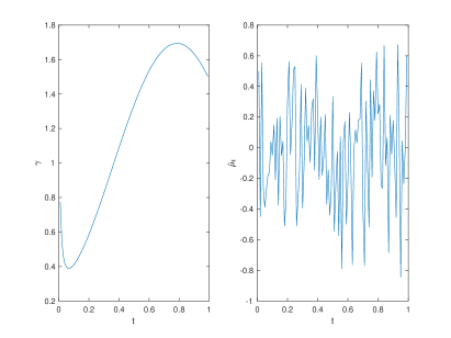
Figure 1.

Figure 1: The path

In order to obtain the effect of delay, comparison of value function is made. Since the valuation function is a expectation, the simulations are repeated $100$ times.

	$\mathbb{E}-\int_{0}^{T}(v(t)-a(t))^{2}dt$	$\mathbb{E}x(t)$	$J(v)$
$\delta=0.48$	-4.5873	2.0301	-2.5573
$\delta=0.44$	-4.3558	2.0900	-2.2658
$\delta=0.42$	-3.7601	2.0890	-1.6711
$\delta=0.40$	-3.1938	2.0874	-1.1063
$\delta=0.38$	-2.7869	2.0874	-0.6919

Table 1: The effect of the delay term

One point of interest is the performance of the deviation from $v(t)$ and psychological expectation level $a(t)$ becomes smaller as delay becomes smaller, and the value function becomes larger. In short, the delay leads to decreased value function.

References

- [1] A. Bensoussan, Stochastic Control of Partially Observable Systems. Cambridge: Cambridge University Press, 1992.
- [2] L. Chen, Z. Wu, Maximum principle for the stochastic optimal control problem with delay and application, Automatica, 46 , 1074-1080. 2010.
- [3] J. Huang, X. Li and J. Shi, Forward-backward linear quadratic stochastic optimal control problem with delay, Systems & Control Letters, 61, 623-630, 2012.
- [4] J. Huang, G. C. Wang, and J. Xiong, A maximum principle for partial information backward stochastic control problems with applications, SIAM J. Control Optim., Vol. 48(4), 2106-2117, 2009.
- [5] S. Lenhart, J. Xiong, J. Yong, Optimal controls for stochastic partial differential equations with an application in population modeling. SIAM J. Control Optim., Vol. 54, 495-535, 2016.
- [6] N. Li, G. C. Wang and Z. Wu, Linear-quadratic optimal control for time-delay stochastic system with recursive utility under full and partial information. Automatica J. IFAC 121, 109169, 2020.
- [7] B. Øksendal, A. Sulem, Maximum principles for optimal control of forward-backward stochastic differential equations with jumps, SIAM J. Control Optim., Vol. 48(5), 2945-2976, 2009.
- [8] B. Øksendal, A. Sulem, T. Zhang, Optimal control of stochastic delay equations and time-advanced backward stochastic differential equations. Adv. Appl. Probab., Vol. 43(2), 572-596, 2011.
- [9] S. Tang, The maximum principle for partially observed optimal control of stochastic differential equations, SIAM J. Control Optim., Vol. 36, 1596-1617, 1998.
- [10] G. C. Wang and Z. Wu, Kalman-Bucy filtering equations of forward and backward stochastic systems and applications to recursive optimal control problems. J. Math. Anal. Appl. 342, no. 2, 1280-1296, 2008.
- [11] G. C. Wang, Z. Wu, J. Xiong. Maximum Principle for Forward-Backward Stochastic Control Systems with Correlated State and Observation Noises. SIAM J. Control Optim., Vol. 51(1), 491-524, 2013.
- [12] G. C. Wang, Z. Wu and J. Xiong. A linear-quadratic optimal control problem of forward-backward stochastic differential equations with partial information. IEEE Trans. Automat. Control 60, no. 11, 2904–2916, 2015.
- [13] G. C. Wang, C. Zhang, and W. Zhang, Stochastic maximum principle for mean-field type optimal control with partial information, IEEE Trans. Automat. Control, Vol. 59, 522-528, 2014.
- [14] X. Y. Zhou, On the necessary conditions of optimal controls for stochastic partial differential equations, SIAM J. Control Optim., Vol. 31, 1462-1478, 1993.
- [15] J. Zhang. A numerical scheme for BSDES. The Annals of Applied Probability, Vol. 14, 459-488, 2004.
- [16] Q. Zhang, Controlled partially observed diffusions with correlated noise, Appl. Math. Optim., Vol. 22, 265-285, 1990.
- [17] S. Zhang, J. Xiong. A numerical method for forward-backward stochastic equations with delay and anticipated term. Statistics and Probability Letters, Vol. 149, 107–115, 2019.
- [18] S. Zhang, J. Xiong, X. Liu. Stochastic maximum principle for partially observed forward-backward stochastic differential equations with jumps and regime switching, Sci. China Inf. Sci. 61, 70211, 2018.
- [19] X. Y. Zhou, On the necessary conditions of optimal controls for stochastic partial differential equations, SIAM J. Control Optim., Vol. 31, 1462-1478, 1993.