Stationary States of the One-dimensional Facilitated Asymmetric Exclusion Process

Abstract

We describe the translation invariant stationary states (TIS) of the one-dimensional facilitated asymmetric exclusion process in continuous time, in which a particle at site $i\in\mathbb{Z}$ jumps to site $i+1$ (respectively $i-1$) with rate $p$ (resp. $1-p$), provided that site $i-1$ (resp. $i+1$) is occupied and site $i+1$ (resp. $i-1$) is empty. All TIS states with density $\rho\leq 1/2$ are supported on trapped configurations in which no two adjacent sites are occupied; we prove that if in this case the initial state is i.i.d. Bernoulli then the final state is independent of $p$. This independence also holds for the system on a finite ring. For $\rho>1/2$ there is only one TIS. It is the infinite volume limit of the probability distribution that gives uniform weight to all configurations in which no two holes are adjacent, and is isomorphic to the Gibbs measure for hard core particles with nearest neighbor exclusion.

Keywords: Asymmetric facilitated exclusion processes, one dimensional conserved lattice gas, facilitated jumps, translation invariant steady states, asymmetry independence, F-ASEP, F-TASEP

AMS subject classifications: 60K35, 82C22, 82C23, 82C26

1 Introduction

The facilitated exclusion process is a model of particles moving on a lattice, which we take to be $\mathbb{Z}^{d}$. Our primary interest is in the one-dimensional version in which particles hop only to nearest neighbor sites, but for completeness we first describe the general model. A configuration of the model is an arrangement of particles on $\mathbb{Z}^{d}$, with each site either empty or occupied by a single particle. If site $i$ is occupied, and one of its neighboring sites is also, then the particle at site $i$ attempts, at rate 1, to jump to another site $j$, succeeding only if the target is unoccupied. The target site $j$ is chosen with probability $\pi(j-i)$, where $\pi:\mathbb{Z}^{d}\to\mathbb{R}_{+}$ is some probability distribution: $\pi\geq 0$ and $\sum_{j\in\mathbb{Z}^{d}}\pi(j)=1$.

We will generally consider states of the system—probability measures on the set of configurations—which have a well-defined density $\rho$, in the sense that, with probability one, a fraction $\rho$ of the sites in each configuration are occupied (see (1.1) for a precise statement). (Here, and throughout unless stated otherwise, by “measure” we mean “probability measure.”) Since particles are neither created nor destroyed, the density is a conserved quantity. If $\rho$ is not too large there will exist frozen configurations in which no two adjacent sites are occupied and hence no particle can move; the maximum density of such a frozen configuration is clearly 1/2.

Most studies of the model with $d\geq 2$ consider the case in which the target sites are uniformly distributed over the nearest neighbors of the jumping particle. For $d=2$, simulations [13, 18, 19] suggest a somewhat surprising property of the model (which presumably holds for $d\geq 2$): there is a critical density $\rho_{c}<1/2$ such that, if the initial state of the models is the measure with Bernoulli i.i.d. marginals (which we will refer to simply as Bernoulli measure) with density $\rho$, then with probability 1, (i) for $\rho<\rho_{c}$ the model eventually reaches a frozen configuration, while (ii) for $\rho>\rho_{c}$ the configuration remains active—that is, particles continue to jump—for all time. Note that when $\rho_{c}<\rho\leq 1/2$ there exist frozen configurations with density $\rho$; these are traps for the dynamics, but with probability 1 they are avoided. To obtain such a result rigorously, or indeed any interesting rigorous results, seems very challenging (but see [20]). Indeed, we are not able to prove what seems to be self evident: that the configurations eventually freeze for sufficiently small $\rho$, say $\rho<10^{-23}$.

In the remainder of this paper we consider only the case $d=1$, with probabilities $p$ and $1-p$ of jumps to the right and left, respectively (that is, we take $\pi(1)=p$, $\pi(-1)=1-p$, and $\pi(j)=0$ for $j\neq\pm 1$). See Figure 1. This model is the Facilitated Asymmetric Simple Exclusion Process (F-ASEP), with special cases $p=0,1$ (Totally Asymmetric, the F-TASEP) [1, 2, 5, 7, 8] and $p=1/2$ (Symmetric, the F-SSEP) [3, 6]. A discrete time version of the F-TASEP was studied in [10, 11]. We write $X=\{0,1\}^{\mathbb{Z}}$ for the configuration space; the condition that configuration $\eta$ have density $\rho$ is now

$$\lim_{N\to\infty}\frac{1}{N}\sum_{i=1}^{N}\eta_{i}=\lim_{N\to\infty}\frac{1}{N}\sum_{i=-N}^{-1}\eta_{i}=\rho,$$ (1.1)

and we let $X_{\rho}$ denote the set of such configurations. We let $F\subset X$ denote the set of frozen configurations.

Figure 1: Transitions in the one-dimensional F-TASEP

We will study the translation invariant (TI) measures on $X$ which are stationary for the dynamics (TIS measures); for this purpose it suffices to consider extremal TIS measures, that is, the set of measures such that every TIS measure is a convex combination of these, and none of these is a proper convex combination of others. As we show below, each extremal measure will be supported on $X_{\rho}$ for some value of $\rho$. The stationary measures for the symmetric case were discussed, for finite volume, in [6]; the results given there carry over smoothly to infinite volume. The current paper contains two main results, one each for low density ($0<\rho<1/2)$ and high density ($1/2<\rho<1$), discussed in Sections 3 and 4, respectively.

For $0<\rho<1/2$, the set of TIS states is simple: all such states are frozen, that is, are supported on $F$, and all TI measures on $F$ are TIS measures. In this case we pose and answer the question: if the initial state is Bernoulli, what is the final state? Our main result is that this final state is independent of the asymmetry parameter $p$. Moreover, it is also the final state arising from an initial Bernoulli measure for the discrete-time F-TASEP, in which all particles attempt to jump at the same times [10, 11]. However, the independence of the degree of asymmetry does not hold for discrete-time dynamics [12].

For $1/2<\rho<1$ we prove that there is a unique TIS state for each value of $\rho$. This state may in fact be identified as the Gibbs measure for a statistical mechanical system in which the only interaction is an exclusion rule that forbids two adjacent empty sites. Results identifying stationary states of particle systems with Gibbs measures have been established earlier [9, 24], but under the assumption that the transition rates for the particle system satisfy a detailed balance condition, which those of the F-ASEP do not (unless $p=1/2$).

Our proof of the uniqueness relies on a coupling with the well-studied Asymmetric Simple Exclusion Model (ASEP). The TIS states of density $\hat{\rho}$ for the latter are precisely the Bernoulli measures [17] (if $p\neq 1/2$ there are also non-TI stationary states, which are not relevant for our discussion here). Our coupling yields a correspondence between these states and the TIS states of the F-ASEP with density $\rho=1/(2-\hat{\rho})$.

Our coupling, from the ASEP to the F-ASEP, is a bit more complicated than the simple map, from the F-ASEP to the ASEP, used in [1]. That map requires that the particles be labeled, and translation invariant measures for labeled particle configurations can’t be normalized. Thus the map in [1] is not well suited for our problem of finding the translation invariant stationary probability measures for the F-ASEP. We therefore use a coupling that does not require labeling.

2 The model

In this section we give various definitions and simple results which will be needed later, and first mention several pieces of general notation. For any sets $A$ and $B$, function $f:A\to B$, and measure $\lambda$ on $A$ we let $f_{*}\lambda$ be the measure on $B$ with $(f_{*}\lambda)(C)=\lambda(f^{-1}(C))$; moreover, if $B=\mathbb{R}$ we let $\lambda(f)=\int_{A}f\,d\lambda$ denote the expected value of $f$ under $\lambda$. When $C\subset B$ we let ${\bf 1}_{C}:B\to\{0,1\}$ denote the indicator function of the set $C$; we will omit mention of the set $B$ when this is clear from the context, as it usually is. If $S$ is a finite set then $|S|$ denotes the size of $S$.

We now turn to the models under consideration. As indicated above, the configuration space of the F-ASEP model is $X:=\{0,1\}^{\mathbb{Z}}$. (In Section 3.2 we will consider also the same dynamics on a ring of $L$ sites with periodic boundary conditions; any notation specific to that case will be introduced as needed). Let $F\subset X$ denote the set of frozen configurations in which no two adjacent sites are occupied, and similarly let $G\subset X$ denote the set of configurations with no two adjacent empty sites. We write $\eta=(\eta(i))_{i\in\mathbb{Z}}$ for a typical configuration, and for $j,k\in\mathbb{Z}$ with $j\leq k$ we let $\eta\hbox{$(j\!:\!k)$}=(\eta(i))_{j\leq i\leq k}$ denote the portion of the configuration lying between sites $j$ and $k$ (inclusive). We will occasionally use string notation for configurations or partial configurations, writing for example $\eta\hbox{$(0\!:\!4)$}=\eta(0)\cdots\eta(4)=10100=(10)^{2}0$.

We denote by $\tau$ the translation operator: if $\eta\in X$ then $(\tau\eta)(i)=\eta(i-1)$, if $f$ is any function on $X$ then $\tau f(\eta)=f(\tau^{-1}\eta)$, and if $\mu$ is a (Borel) measure on $X$ then $\tau$ acts on $\mu$ as $\mu\mapsto\tau_{*}\mu$. We let ${\cal L}(X)$ denote the space of functions $f:X\to\mathbb{R}$ for which $f(\eta)$ depends on the values $\eta(k)$ for only finitely many sites $k$, ${\cal C}(X)$ denote the space of real-valued continuous functions on $X$ (for the topology generated by ${\cal L}(X)$), and ${\cal M}={\cal M}(X)$ denote the space of translation invariant probability measures on $X$ (equipped with the Borel $\sigma$-algebra, i.e., the natural product $\sigma$-algebra, on $X$).

We now turn to a formal specification of the system. The dynamics is controlled by Site Associated Poisson Processes (SAPPs); two of these, controlling rightward and leftward jumps, respectively, are associated with each site $i\in\mathbb{Z}$. Specifically, given a TI measure $\mu\in{\cal M}$ which specifies the initial distribution of the system, we consider the probability space $(\Omega,{\bf P}_{p}^{\mu})$:

$$\Omega =X\times\Omega_{0},\quad\text{with}\quad\Omega_{0}=\prod_{i\in\mathbb{Z}}\bigl{(}{\cal T}^{(i,r)}\times{\cal T}^{(i,l)}\bigr{)},$$ (2.1)

$${\bf P}_{p}^{\mu} =\mu\times{\bf P}_{p},\quad\text{with}\quad{\bf P}_{p}=\prod_{i\in\mathbb{Z}}\bigl{(}\lambda_{p}^{(i,r)}\times\lambda_{p}^{(i,l)}\bigr{)}.$$

Here, for $i\in\mathbb{Z}$ and $\#=l$ or $r$,

$${\cal T}^{(i,\#)}=\Bigl{\{}\bigl{(}(i,t^{(i,\#)}_{j})\bigr{)}_{j=1,2,\ldots}\,\Big{|}\,\text{$0<t^{(i,\#)}_{1}<t^{(i,\#)}_{2}\cdots$, $\lim_{j\to\infty}t^{(i,\#)}_{j}=\infty$}\Bigr{\}},$$ (2.2)

and under $\lambda_{p}^{(i,r)}$ (respectively $\lambda_{p}^{(i,l)}$) the points of ${\cal T}^{(i,r)}$ (respectively ${\cal T}^{(i,l)})$ are distributed as a Poisson process of rate $p$ (respectively $1-p$.)

The configuration now evolves as follows: at each time $t=t^{(i,r)}_{j}$ a particle jumps from site $i$ to site $i+1$ if $\eta_{t-}(i-1)=\eta_{t-}(i)=1-\eta_{t-}(i+1)=1$, and at each time $t=t^{(i,l)}_{j}$ a particle jumps from $i$ to $i-1$ if $\eta_{t-}(i+1)=\eta_{t-}(i)=1-\eta_{t-}(i-1)=1$. This so-called Harris graphical construction (or Poisson construction in [23]) leads [23] to a process $\eta_{t}$, well-defined on $\Omega$, with generator $L$ which acts on ${\cal L}(X)$ via

$$Lf(\eta) =\sum_{i\in\mathbb{Z}}c(i,\eta)[f(\eta^{i,i+1})-f(\eta)].$$ (2.3)

Here $\eta^{i,j}$ denotes the configuration $\eta$ with the values of $\eta(i)$ and $\eta(j)$ exchanged. The rates $c(i,\eta)$ are given by

$$c(i,\eta)=\begin{cases}p,&\hbox{if $\eta(i-1)=\eta(i)=1$ and $\eta(i+1)=0$,}\\ 1-p,&\hbox{if $\eta(i)=0$ and $\eta(i+1)=\eta(i+2)=1$,}\\ 0,&\hbox{otherwise.}\end{cases}$$ (2.4)

$L$ is the generator of a Markov semigroup $S(t)=e^{Lt}$ on ${\cal C}(X)$, which thus acts on ${\cal M}(X)$ via $\mu\to\mu_{t}=\mu S(t)$, where $(\mu S(t))(f)=\mu(S(t)f)$ or equivalently $(\mu S(t))(A)=\int_{X}Q_{t}(\eta,A)\,d\mu$, with $Q_{t}(\eta,A)=(S(t){\bf 1}_{A})(\eta)$ the transition kernel of the Markov process. We will assume that this process, and others to be considered later, have right-continuous sample paths.

Remark 2.1.

Since the set of all Poisson times for different sites will a.s. be dense in $(0,\infty)$, one cannot perform all the particle jumps in temporal order, and some care is needed to show that the construction is well defined. Details are given in [23, Sections 4.3 and 4.4]. Later we carry out such a construction with a different but equivalent definition of the dynamics, in which the Poisson times at which particles can jump are associated with the particles rather than with the sites (Particle Associated Point Processes). See the proof of Theorem 4.3.

If $\mu$ is a TI measure on $X$ then, by the ergodic theorem, $\mu$-almost every configuration $\eta$ has a density, i.e.,

$$r(\eta)=\lim_{N\to\infty}\frac{1}{2N+1}\sum_{i=-N}^{N}\eta(i)$$ (2.5)

exists almost surely. (2.5) defines a map $r:X\to[0,1]$; we will say that a TI measure $\mu$ has density $\rho$ if $r(\eta)=\rho$ $\mu$-a.s. Note that if $\mu$ has density $\rho$ then $\mu(\eta(i))=\rho$ for any $i$, but that the former is a stronger statement, ruling out, for example, the possibility that $\mu$ is a superposition of measures of different densities. The next lemma shows that in seeking to describe the set of all stationary TI measures $\mu$ it suffices to consider those for which $\mu(F)$ is 0 or 1 and for which $r(\eta)$ is $\mu$-a.s. constant.

Lemma 2.2.

Every TIS measure $\mu$ on $X$ is a convex combination of TIS measures for which $r$ is a.s. constant and $F$ has measure 0 or 1.

Proof.

Let $\nu=r_{*}\mu$; $\nu$ is a measure on $[0,1]$ which gives the distribution of the density under $\mu$. Then (see for example [16]) there exists a regular conditional probability distribution for $\mu$, that is, a family $\{\mu_{\rho}\mid\rho\in[0,1]\}$ of probability measures on $X$ such that $\mu_{\rho}$ has density $\rho$ and for any measurable $A\subset X$,

$$\mu(A)=\int_{0\leq\rho\leq 1}\mu_{\rho}(A)d\nu(\rho).$$ (2.6)

Moreover, $\{\mu_{\rho}\}$ is unique in the sense that for any other such family $\{\mu^{\prime}_{\rho}\}$, $\mu_{\rho}=\mu^{\prime}_{\rho}$ $\nu$-a.s. If we further write $\mu_{\rho}=\mu_{\rho}\big{|}_{F}+\mu_{\rho}\big{|}_{X\setminus F}$ we obtain, after normalization, the desired representation. It remains to verify that these normalized measures, $\mu_{\rho}\big{|}_{F}\big{/}\bigl{(}\mu_{\rho}\big{|}_{F}(X)\bigr{)}$ and $\mu_{\rho}\big{|}_{X\setminus F}\big{/}\bigl{(}\mu_{\rho}\big{|}_{X\setminus F}(X)\bigr{)}$, are TIS measures.

Now

$$\mu(A)=\tau_{*}\mu(A)=\int_{0\leq\rho\leq 1}\tau_{*}\mu_{\rho}(A)d\nu(\rho),$$ (2.7)

and from (2.5) it follows that $\tau_{*}\mu_{\rho}$ has density $\rho$, so that the uniqueness of the conditional probability distribution implies that $\tau_{*}\mu_{\rho}=\mu_{\rho}$ $\nu$-a.s. Stationarity of $\mu_{\rho}$ $\nu$-a.s. follows similarly from the fact that neither dynamics destroys or creates particles. Finally, translation invariance and stationarity of $\mu_{\rho}\big{|}_{F}$ and $\mu_{\rho}\big{|}_{X\setminus F}$ follows from the fact that $F$ is translation invariant and invariant under the dynamics. ∎

The key idea in the next lemma appears in [6] in the context of a system on a ring.

Lemma 2.3.

If $\mu$ is a TIS measure on $X$ then $\mu(F\cup G)=1$.

Proof.

The argument we give requires that $p$ be strictly positive; by the symmetry of the model under simultaneous spatial reflection and the replacement $p\to 1-p$, we may assume that this condition holds. Suppose that $\mu(F\cup G)<1$. If $\eta\notin F\cup G$ then $\eta$ contains two adjacent zeros and two adjacent ones; let $2k$ be the minimum number of sites by which a double zero follows a double one—that is, for which the string $11(01)^{k}00$ occurs in a configuration—with nonzero probability. We first note that $k\geq 1$ almost surely. For from (2.4), the translation invariance of $\mu$, and $\mu=\mu_{t}$ for all $t$,

$$\frac{d}{dt}\mu\bigl{(}\eta(0{:}1)=11\bigr{)} =-p\,\mu\bigl{(}\eta(0{:}2)=110\bigr{)}-(1-p)\,\mu\bigl{(}\eta(-1{:}1)=011\bigr{)}$$

$$\hskip 30.0pt+p\,\mu\bigl{(}\eta(-2{:}1)=1101\bigr{)}+(1-p)\,\mu\bigl{(}\eta(0{:}3)=1011\bigr{)}$$

$$=-p\,\mu\bigl{(}\eta(0{:}3)=1100\bigr{)}-(1-p)\,\mu\bigl{(}\eta(-2{:}1)=0011\bigr{)}.$$

This quantity must vanish, since $\mu$ is stationary, and since $p$ is nonzero the probability of $1100$ occurring is zero.

Now by the choice of $k$, $\mu\bigl{(}\eta(0{:}2k+3)=11(01)^{k}00\bigr{)}>0$. Then a simple calculation as above, using repeatedly the fact that for any $i$ and for $j<k$, $\mu\bigl{(}\eta(i{:}i+2j+3)=11(01)^{j}00\bigr{)}=0$, shows that

$$\frac{d}{dt}\mu\bigl{(}\eta(2{:}2k+3)=11(01)^{(k-1)}00\bigr{)}=p\,\mu\bigl{(}\eta(0{:}2k+3)=11(01)^{k}00\bigr{)}>0,$$ (2.8)

contradicting stationarity.∎

Remark 2.4.

Let $\eta^{*}\in X$ be the period-two configuration defined by $\eta^{*}(i)=i\bmod 2$. $\eta^{*}$ and its translate $\tau\eta^{*}$ consist of alternating 1’s and 0’s, and the measure $\mu^{*}=(\delta_{\eta^{*}}+\delta_{\tau\eta^{*}})/2$ is a TIS measure with density $\rho=1/2$. Note that $\mu^{*}(F)=\mu^{*}(G)=1$.

Theorem 2.5.

Let $\mu$ be a TIS measure on $X$ with density $\rho$. Then:

(a) If $\rho<1/2$ then $\mu(F)=1$, i.e., $\mu$ is supported on $F$.

(b) If $\rho=1/2$ then $\mu=\mu^{*}$ (see Remark 2.4).

(c) If $\rho>1/2$ then $\mu(G)=1$, i.e., $\mu$ is supported on $G$.

Proof.

We know that $\mu$ is supported on $F\cup G$. Suppose that $\eta\in\mathop{\rm supp}\mu$; then we may assume that $\eta\in F\cup G$ and $r(\eta)=\rho$. If $\rho=r(\eta)<1/2$ then, by (2.5), $\eta$ must contain a positive density of double zeros and so lie in $F\setminus G$, verifying (a); similarly, if $\rho>1/2$ then $\eta\in G\setminus F$, verifying (c). If $\rho=1/2$ then (2.5) with $\eta\in F\cup G$ implies that $\eta$ does not have a positive density of either double ones or double zeros, and hence almost surely has no double ones or double zeros at all, verifying (b). ∎

3 The low density region

In this section we consider TIS states on $X_{\rho}$ with $0<\rho<1/2$; by Theorem 2.5 these are necessarily supported on $F$. In fact, any TI measure supported on $F$ is clearly a TIS state; in Remark 4.2 we obtain a prescription for obtaining all such states from a construction introduced there for the study of the high density region. Here we address the following question:

Question 3.1.

If the system is given an initial measure $\mu^{(\rho)}$, the Bernoulli measure with density $0<\rho<1/2$, what is the final measure?

3.1 The totally asymmetric model

In this section we address Question 3.1 for the totally asymmetric model (F-TASEP); we take $p=1$ in (2.4) but the discussion for $p=0$ would be similar. The answer is given in [10, 11] for the discrete-time F-TASEP, and the analysis there applies almost unchanged in the continuous-time case, so we content ourselves with a brief summary.

First, it is convenient to enlarge the state space of the process from $X$ to $\widehat{X}:=X\times\mathbb{Z}$, writing the state of the system at time $t$ as $(\eta_{t},J_{t})$. In this new version of the model, $J_{t}$ is the signed count of the number of particles passing between sites 0 and 1 up to time $t$. The new version is defined on the same probability space $(\Omega,{\bf P}_{p}^{\mu})$ as the original one (see (2.1), (2.2)), with $J_{t}$ incremented or decremented by 1 at, and only at, those times $t^{(0,r)}_{j}$ or $t^{(1,l)}_{j}$, respectively, at which jumps actually occur; it is straightforward to verify, as in [23], that this leads to a well-defined process. We always assume that $J_{0}=0$.

The variable $J_{t}$ allows us to introduce the height profile $h_{t}:\mathbb{Z}\to\mathbb{Z}$ associated with the pair $(\eta_{t},J_{t})\in\widehat{X}$ (see, e.g., [15]), defined by the requirements that $h_{t}(i)-h_{t}(i-1)=1-2\eta_{t}(i)=(-1)^{\eta_{t}(i)}$ for all $i\in\mathbb{Z}$ and $h_{t}(0)=2J_{t}$, or more explicitly by

$$h_{t}(i)=\begin{cases}2J_{t}+\displaystyle\sum_{j=1}^{i}(-1)^{\eta_{t}(j)},&\hbox{if $i\geq 0$,}\\ \vskip 3.0pt\cr 2J_{t}-\displaystyle\sum_{j=i+1}^{0}(-1)^{\eta_{t}(j)},&\hbox{if $i<0$.}\end{cases}$$ (3.1)

Then, since $0<\rho<1/2$, $\lim_{i\to\pm\infty}h_{t}(i)=\pm\infty$. Moreover, as a function of $t$, $h_{t}$ is monotonically increasing; in particular, $h_{t}(i)$ increases by 2 when a particle jumps from site $i$ to site $i+1$, and such an increase can occur only if $h_{t}(i-1)>h_{t}(i)$. See the inset in Figure 2.

We can now sketch the determination of the fate of an arbitrary initial configuration $\eta_{0}\in X_{\rho}$; full details are given in [11]. Define $Q=Q(\eta_{t})\subset\mathbb{Z}$ by $Q:=\{q\in\mathbb{Z}\mid h_{t}(q)>\sup_{i<q}h_{t}(i)\}$. From the observation above on how $h_{t}$ can increase it follows that $Q(\eta_{t})$ is in fact independent of $t$ and that for $q\in Q$, $h_{t}(q)$ is constant. If $q$ and $q^{\prime}$ are consecutive elements of $Q$ and $i\in\mathbb{Z}$ satisfies $q\leq i<q^{\prime}$, then $h_{t}(i)<h_{t}(q^{\prime})=h_{0}(q^{\prime})$, so that $\lim_{t\to\infty}h_{t}(i)$, and hence also $\eta_{\infty}(i)=\lim_{t\to\infty}\eta_{t}(i)$, exist. Further, since $i+h_{0}(i)$ is even for all $i$ and $h_{0}(q^{\prime})-h_{0}(q)=1$, $q^{\prime}-q$ is odd, and so necessarily

$$\eta_{\infty}\hbox{$(q+1\!:\!q^{\prime})$}=1\,0\,1\,0\,\cdots\,1\,0\,0=(1\,0)^{(q^{\prime}-q-1)/2}0.$$ (3.2)

See Figure 2. This completes the determination of $\eta_{\infty}$.

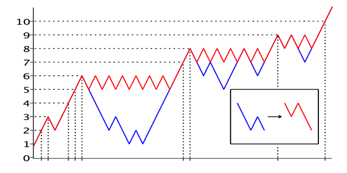
Figure 2: Portion of typical initial (blue, lower) and final (red, upper) height profiles in the F-TASEP; the profile increases monotonically in time from the former to the latter. The vertical dotted lines are at sites in $Q$. The inset shows the local change in the profile associated with the jump of a single particle, carrying local configuration $1\,1\,0\,1$ to $1\,0\,1\,1$.

We now suppose that $\eta_{0}$ is distributed according to the Bernoulli distribution $\mu^{(\rho)}$, and write ${\bf P}_{p}^{(\rho)}$ rather than ${\bf P}_{p}^{\mu^{(\rho)}}$. We ask for the distribution $\mu^{(\rho)}_{\infty}=\eta_{\infty*}{\bf P}_{p}^{(\rho)}$ of $\eta_{\infty}$, where here we think of $\eta_{\infty}$ as a map $\eta_{\infty}:\Omega\to X_{\rho}$. Let $V=\{\eta\in X\mid 0\in Q(\eta)\}$; note that (3.2) implies that $V$ coincides, up to a set of $\mu^{(\rho)}_{\infty}$-measure zero, with $\{\eta\mid\eta\hbox{$(-1\!:\!0)$}=0\,0\}$, and with $\mu^{(\rho)}_{\infty}\bigl{(}\{\eta\mid\eta\hbox{$(-1\!:\!0)$}=1\,1\}\bigr{)}=0$ this implies that $\mu^{(\rho)}_{\infty}(V)=1-2\rho$. To obtain $\mu^{(\rho)}_{\infty}$ we will first describe the conditional measure $\mu^{(\rho)}_{\infty}(\cdot\mid V)$, then obtain $\mu^{(\rho)}_{\infty}$ as the (unique) TI measure with this conditional measure. For $\eta_{0}\in V$ we may index $Q=Q(\eta_{0})$ as $Q=\{q_{k}\}_{k\in\mathbb{Z}}$, taking $q_{0}=0$ and requiring that the $q_{k}$ be increasing in $k$; then we may specify $\mu^{(\rho)}_{\infty}(\cdot\mid V)$ by giving the joint distribution of the variables $n_{k}$ defined by $q_{k+1}-q_{k}=2n_{k}+1$.

It is easy to see that the $n_{k}$ are i.i.d. To describe the distribution of a single $n_{k}$ we recall the Catalan numbers [22]

$$c_{n}=\frac{1}{n+1}\binom{2n}{n},\quad n=0,1,2,\ldots\,;$$ (3.3)

$c_{n}$ counts the number of strings of $n$ 0’s and $n$ 1’s in which the number of 0’s in any initial segment does not exceed the number of 1’s. If $q=q_{k}\in Q$ and $l=q+2n+1$ then $q_{k+1}=l$ if and only if $h_{0}(l)=h_{0}(q)+1$ and $h_{0}(i)\leq h_{0}(q)$ for $q<i<l$, and there are $c_{n}$ strings $\eta\hbox{$(q+1\!:\!l-1)$}$ satisfying this condition and hence yielding $q_{k+1}=l$. Since each such string has probability $\rho^{n}(1-\rho)^{n+1}$ we have sketched a proof of the next theorem, which is taken from [11]. Recall that $\tau$ denotes translation and ${\bf 1}_{C}$ the indicator function of $C$.

Theorem 3.2.

(a) The random variables $n_{k}$ of the F-TASEP, defined on $V$ as above, are i.i.d. under $\mu^{(\rho)}_{\infty}(\cdot\mid V)$, with distribution

$$\mu^{(\rho)}_{\infty}(\{n_{k}=n\}\mid V)=c_{n}\rho^{n}(1-\rho)^{n+1},\quad n=0,1,2,\ldots.$$ (3.4)

(b) The measure $\mu^{(\rho)}_{\infty}$ is given by

$$\mu^{(\rho)}_{\infty}=\frac{1}{Z}\sum_{m\geq 0}\sum_{i=0}^{2m}\tau_{*}^{-i}\bigl{(}{\bf 1}_{V_{m}}\mu^{(\rho)}_{\infty}(\cdot\mid V)\bigr{)}=\sum_{m\geq 0}\sum_{i=0}^{2m}\tau_{*}^{-i}\bigl{(}{\bf 1}_{V_{m}}\mu^{(\rho)}_{\infty}\bigr{)},$$ (3.5)

where $V_{m}=\{\eta_{0}\in V\mid q_{1}-q_{0}=2m+1\}$ and $Z=\mu^{(\rho)}_{\infty}(V)^{-1}$ is a normalizing constant.

3.2 The model in finite volume

In this section we address Question 3.1, or rather an appropriately modified version of it, for the F-ASEP on a periodic ring of $L$ sites. The system size $L$ will be constant during our analysis and we typically suppress $L$-dependence. We first discuss the totally asymmetric model and describe the result corresponding to Theorem 3.2, then show that the limiting measure is in fact independent of the asymmetry parameter $p$. The ring is denoted $\mathbb{Z}_{L}:=\{0,1,\ldots,L-1\}$; we consider a system of $N$ particles on these sites, governed by the obvious modification of the F-ASEP dynamics defined in Section 2. For a configuration $\eta\in\{0,1\}^{\mathbb{Z}_{L}}$ we let $|\eta|:=\sum_{i=1}^{L}\eta(i)$ denote the number of particles in $\eta$; the configuration space of our model is then $X^{(N)}:=\{\eta\in\{0,1\}^{\mathbb{Z}_{L}}\mid|\eta|=N\}$. We will be interested in the fate of an initial measure $\mu^{(N)}$ which is uniform on $X^{(N)}$; the probability space is then $(\Omega^{(N)},{\bf P}_{p}^{(N)})$:

$$\Omega^{(N)} =X^{(N)}\times\prod_{i\in\mathbb{Z}_{L}}\bigl{(}{\cal T}^{(i,r)}\times{\cal T}^{(i,l)}\bigr{)},$$ (3.6)

$${\bf P}_{p}^{(N)} =\mu^{(N)}\times\prod_{i\in\mathbb{Z}_{L}}\bigl{(}\lambda_{p}^{(i,r)}\times\lambda_{p}^{(i,l)}\bigr{)}.$$

Here ${\cal T}$ and $\lambda$ are as in (2.1). (In view of our earlier use of $\mu^{(\rho)}$ and ${\bf P}_{p}^{(\rho)}$, writing $\mu^{(N)}$ and ${\bf P}_{p}^{(N)}$ is admittedly an abuse of notation, but we believe that this will not give rise to confusion.) The construction of the dynamics is parallel to the construction in infinite volume, but is technically simpler because the considerations of Remark 2.1 do not apply; we omit details. The auxiliary variable $J_{t}$ is not needed here.

Now consider the F-TASEP, taking $p=1$ above. Given an initial configuration $\eta_{0}\in\{0,1\}^{\mathbb{Z}_{L}}$, with $|\eta_{0}|<L/2$, we extend $\eta_{0}$ to an $L$-periodic configuration $\eta_{0}^{*}$ on $\mathbb{Z}$, apply the construction of Section 3.1 to obtain $Q(\eta_{0}^{*})$, and let $Q(\eta_{0}):=Q(\eta^{*}_{0})\cap\{0,1,\ldots,L-1\}$; $Q(\eta_{0})$ will contain $L-2|\eta_{0}|$ sites. An argument as in infinite volume shows that the limiting configuration $\eta_{\infty}$ exists and satisfies (3.2) for $q,q^{\prime}$ consecutive (in cyclic order) elements of $Q(\eta_{0})$ (with the expression $q^{\prime}-q-1$ in the exponent of (3.2) interpreted mod $L$).

Now fix $N<L/2$; we will determine the distribution $\mu^{(N)}_{\infty}=\eta_{\infty*}{\bf P}_{p}^{(N)}$ of $\eta_{\infty}$ when $\eta_{0}$ is distributed according to $\mu^{(N)}$ (this is the modified version of Question 3.1 referred to above). Let $V^{(N)}:=\{\eta\in X^{(N)}\mid 0\in Q(\eta)\}$ and note that $|V^{(N)}|=(L-2N)\binom{L}{N}/L$, since if one partitions $X^{(N)}$ into equivalence classes under translation then each class contains a fraction $(L-2N)/L$ of elements belonging to $V^{(N)}$. We can determine the conditional measure $\mu^{(N)}_{\infty}(\cdot\mid V^{(N)})$ by simple counting: given $0=q_{0}<q_{1}<\ldots<q_{L-2N-1}\leq L-1$, with $q_{i+1}-q_{i}\equiv 2n_{i}+1\pmod{L}$ for $0\leq n_{i}<L/2$, there are $\prod_{i=0}^{L-2N-1}c_{n_{i}}$ initial configurations $\eta_{0}\in X^{(N)}$ with $Q(\eta_{0})=\{q_{0},\ldots,q_{L-2N-1}\}$, all leading to $\eta_{\infty}=\eta^{(q_{0},\ldots,q_{L-2N-1})}$, where

$$\eta^{(q_{0},\ldots,q_{L-2N-1})}:=(10)^{q_{1}-q_{0}}0(10)^{q_{2}-q_{1}}0\cdots 0(10)^{q_{0}-q_{L-2N-1}+L}0.$$ (3.7)

Thus we have

Theorem 3.3.

(a) The possible limiting configurations of the F-TASEP model on $V^{(N)}$ are the $\eta^{(q_{0},\ldots,q_{L-2N-1})}$, and

$$\mu^{(N)}_{\infty}\bigl{(}\{\eta^{(q_{0},\ldots,q_{L-2N-1})}\}\mid V^{(N)})=\frac{\displaystyle{L\prod\nolimits_{i=0}^{L-2N-1}c_{n_{i}}}}{(L-2N)\binom{L}{N}}.$$ (3.8)

(b) $\mu^{(N)}_{\infty}=\displaystyle{\frac{1}{L}\sum_{i=0}^{L-1}\tau^{i}_{*}\mu^{(N)}_{\infty}(\cdot\mid V^{(N)})}$.

We now consider the general F-ASEP model on $\mathbb{Z}_{L}$, with partially asymmetric dynamics governed by the asymmetry parameter $p$. Since from any initial configuration $\eta_{0}$ there is a sequence of possible transitions leading to a frozen configuration, $\eta_{\infty}=\lim_{t\to\infty}\eta_{t}$ exists almost surely, for any $\eta_{0}$, and is frozen. The distribution $\mu^{(N)}_{\infty}=\eta_{\infty*}{\bf P}_{p}^{(N)}$ of the limiting configurations is then well defined; our goal is to show that this distribution is independent of $p$ (as our notation indicates). The next lemma is simple—it follows immediately from elementary consideration of the dynamics—but will be useful in several places.

Lemma 3.4.

Suppose that $\eta_{t}$ is the state at time $t$ of a process evolving via the F-ASEP dynamics, for a system either of $N$ particles on $L$ sites or in infinite volume. If for some site $i$ and time $t$, $\eta_{t}(i)=\eta_{t}(i+1)=0$, then also $\eta_{s}(i)=\eta_{s}(i+1)=0$ for all $s<t$, respectively ${\bf P}_{p}^{(N)}$ or ${\bf P}_{p}^{(\rho)}$ almost surely.

Lemma 3.4 implies that if two adjacent sites are empty in $\eta_{\infty}$ then they must also be empty in all $\eta_{t}$, $t\geq 0$. Because of this it is convenient to decompose configurations into components—strings of 1’s and 0’s within which no two adjacent sites are empty but which are separated from each other by (at least) two adjacent empty sites. See Figure 3. (Formally a component of a configuration $\eta$ is the restriction $\eta|_{I}$ of $\eta$ to an interval $I=\{i,i+1,\ldots,j\}$ for which $\eta(i)=\eta(j)=1$, $\eta(i-2)=\eta(i-1)=\eta(j+1)=\eta(j+2)=0$, and there is no site $k$ in $I$ such that $\eta(k)=\eta(k+1)=0$.) We let $c(\eta)$ denote the number of components in $\eta$, and write ${\bf P}^{(N,n)}_{p}$ for the measure ${\bf P}_{p}^{(N)}$ conditioned on the event $c(\eta_{0})=n$.

Theorem 3.5.

For all $L$ and $N$, with $N<L/2$, the measure $\mu^{(N)}_{\infty}$ is independent of $p$, and so is given by Theorem 3.3(b).

Proof.

We will prove by induction on $n$, $n=1,2,\ldots$, that for all $L$ and $N$ with $L/2>N\geq n$ the distribution of $\eta_{\infty}$ under ${\bf P}^{(N,n)}_{p}$ is independent of $p$. The theorem then follows from ${\bf P}_{p}^{(N)}(\cdot)=\sum_{n=1}^{N}{\bf P}^{(N,n)}_{p}(\cdot){\bf P}_{p}^{(N)}(c(\eta_{0})=n)$, since the distribution $\mu^{(N)}$ of $\eta_{0}$ is independent of $p$. The case $n=1$ of the induction is trivial: if the initial configuration has a single component then so does the final one, and for any $p$ this component is just $101\cdots 01$ (with $N$ 1’s) and its position will be uniformly distributed over the ring, by translation invariance.

We now assume inductively that $n$ is such that for all $k\leq n$ and all $L,N$ with $L/2>N\geq n$, the distribution of $\eta_{\infty}$ under ${\bf P}^{(N,k)}_{p}$ is independent of $p$. We then fix a configuration $\zeta\in X^{(N)}$ and show that ${\bf P}^{(N,n+1)}_{p}(\eta_{\infty}=\zeta)$ is independent of $p$; we may assume that no two consecutive sites are occupied in $\zeta$, since otherwise this probability is 0. Consider first the case $c(\zeta)>1$; then if necessary we may rotate $\zeta$ (which does not affect the conclusion) to an orientation in which there exists a site $i$, with $3\leq i\leq L-3$, such that $\zeta(0)=\zeta(1)=0$, $\zeta(i)=\zeta(i+1)=0$, and $\zeta(j)=1$ for at least one $j$ in the set $\{2,\ldots,i-1\}$ and at least one $j$ in $\{i+2,\ldots,L-1\}$. Given $i$, we define maps $\pi_{1},\pi_{2}:X^{(N)}\to\bigcup_{0\leq N^{\prime}\leq N}X^{(N^{\prime})}$ by $\pi_{1}\eta=\eta{\bf 1}_{\{2,\ldots,i-1\}}$ and $\pi_{2}\eta=\eta{\bf 1}_{\{i+2,\ldots,L-1\}}$, i.e.,

$$(\pi_{1}\eta)(j) =\begin{cases}\eta(j),&\text{if $2\leq j\leq i-1$,}\\ 0,&\text{if $0\leq j\leq 1$ or $i\leq j\leq L-1$},\end{cases}$$ (3.9)

$$(\pi_{2}\eta)(j) =\begin{cases}\eta(j),&\text{if $i+2\leq j\leq L-1$,}\\ 0,&\text{if $0\leq j\leq i+1$.}\end{cases}$$ (3.10)

See Figure 3.

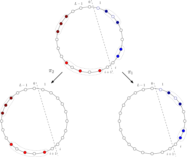
Figure 3: A typical configuration in $E_{2,2}$ (see below) of the finite-volume F-ASEP, with its image under the maps $\pi_{1}$ and $\pi_{2}$. The four components are enclosed in dotted loops and are also indicated by color coding.

For integers $k_{1},k_{2}$ with $1\leq k_{m}\leq|\pi_{m}\zeta|$, satisfying $k_{1}+k_{2}=n+1$, define the events

$$E_{k_{1},k_{2}} :=\{\eta_{0}\in X^{(N)}\mid\eta_{0}(0)=\eta_{0}(1)=\eta_{0}(i)=\eta_{0}(i+1)=0,$$

$$\hskip 75.0pt|\pi_{m}\eta_{0}|=|\pi_{m}\zeta|,\text{ and }c(\pi_{m}\eta_{0})=k_{m},\ m=1,2\},$$

$$E^{(m)}_{k_{m}} :=\{\eta_{0}\in X^{(|\pi_{m}\zeta|)}\mid\eta_{0}=\pi_{m}\eta_{0}\text{ and }c(\eta_{0})=k_{m}\}.$$

We will assume in what follows that $k_{1},k_{2}$ are chosen so that ${\bf P}^{(N,n+1)}_{p}(\eta_{\infty}=\zeta\mid E_{k_{1},k_{2}})\neq 0$. Since

$${\bf P}^{(N,n+1)}_{p}(\eta_{\infty}=\zeta)=\sum_{k_{1},k_{2}}{\bf P}^{(N,n+1)}_{p}(\eta_{\infty}=\zeta\mid E_{k_{1},k_{2}}){\bf P}^{(N,n+1)}_{p}(E_{k_{1},k_{2}})$$ (3.11)

and $E_{k_{1},k_{2}}$ depends only on the initial configuration $\eta_{0}$, it suffices to show that for all such $k_{1},k_{2}$, ${\bf P}^{(N,n+1)}_{p}(\eta_{\infty}=\zeta\mid E_{k_{1},k_{2}})$ is independent of $p$.

Now observe that

$${\bf P}^{(N,n+1)}_{p}(\eta_{\infty}=\zeta\mid E_{k_{1},k_{2}})=\prod_{m=1,2}{\bf P}^{(|\pi_{m}\zeta|,k_{m})}_{p}(\eta_{\infty}=\pi_{m}\zeta\mid E^{(m)}_{k_{m}}).$$ (3.12)

This is because (i) whatever the value of $i$ used to define $\pi_{1}$ and $\pi_{2}$, $\pi_{1}\eta_{0}$ and $\pi_{2}\eta_{0}$ are independent (and hence remain so after conditioning on $E_{k_{1},k_{2}}$), and (ii) since for all histories $\eta_{t}$ arriving at $\eta_{\infty}=\zeta$, Lemma 3.4 implies that the sites $0$, $1$, $i$, and $i+1$ must always be empty, the probability on the left, given $\eta_{0}$, is determined by the SAPP times $t_{j}^{(i^{\prime},\#)}$ for $2\leq i^{\prime}\leq i-1$ and $i+2\leq i^{\prime}\leq L-1$, and these are independent. But also we have

$${\bf P}^{(|\pi_{m}\zeta|,k_{m})}_{p}(\eta_{\infty}=\pi_{m}\zeta\mid E^{(m)}_{k_{m}})=\frac{{\bf P}^{(|\pi_{m}\zeta|,k_{m})}_{p}(\eta_{\infty}=\pi_{m}\zeta)}{{\bf P}^{(|\pi_{m}\zeta|,k_{m})}_{p}(E^{(m)}_{k_{m}})},$$ (3.13)

since, with probability 1 with respect to ${\bf P}^{(|\pi_{m}\zeta|,k_{m})}_{p}$, $\eta_{\infty}=\pi_{m}\zeta$ is possible only if $E^{(m)}_{k_{m}}$ occurs. Both the numerator and denominator on the right hand side of (3.13) are independent of $p$, the numerator by the inductive assumption and the denominator since it involves only the initial condition. Thus ${\bf P}^{(|\pi_{m}\zeta|,k_{m})}_{p}(\eta_{\infty}=\pi_{m}\zeta\mid E^{(m)}_{k_{m}})$ and hence, by (3.12), ${\bf P}^{(N,n+1)}_{p}(\eta_{\infty}=\zeta\mid E_{k_{1},k_{2}})$, are independent of $p$.

This completes the proof of the $p$-independence of ${\bf P}^{(N,n+1)}_{p}(\eta_{\infty}=\zeta)$ in the case $c(\zeta)>1$. From the validity of this result for all such $\zeta$ it follows that

$${\bf P}^{(N,n+1)}_{p}(c(\eta_{\infty})=1)=1-\sum_{l=2}^{N}\sum_{\{\zeta\mid c(\zeta)=l\}}{\bf P}^{(N,n+1)}_{p}(\eta_{\infty}=\zeta)$$ (3.14)

is also independent of $p$. Then by translation invariance, ${\bf P}^{(N,n+1)}_{p}(\eta_{\infty}=\zeta)={\bf P}^{(N,n+1)}_{p}(c(\eta_{\infty})=1)/L$ if $c(\zeta)=1$. This completes the proof. ∎

3.3 The partially asymmetric model in infinite volume

In this section we return to the ($p$-dependent) F-ASEP dynamics on $\mathbb{Z}$; we assume that $\eta_{0}$ is distributed as the Bernoulli measure $\mu^{(\rho)}$, $0<\rho<1/2$, and show that the distribution of the limiting configuration $\eta_{\infty}$ is independent of $p$. As in Section 3.1 we write ${\bf P}_{p}^{(\rho)}$ for the measure ${\bf P}_{p}^{\mu^{(\rho)}}$ on the sample space $\Omega$ of (2.1). We begin with two preliminary results; the first is standard.

Lemma 3.6.

If $f:\Omega\to X$ commutes with translations then $f_{*}{\bf P}_{p}^{(\rho)}$ is mixing under translations.

Proof.

Note that $\Omega$ is in fact a product space, $\Omega=\prod_{i\in\mathbb{Z}}\bigl{(}\{0,1\}\times{\cal T}^{(i,r)}\times{\cal T}^{(i,l)}\bigr{)}$, and that ${\bf P}_{p}^{(\rho)}$ is a product measure. Thus ${\bf P}_{p}^{(\rho)}$ is certainly mixing under translations. Then for any measurable sets $A,B\subset X$,

$$\lim_{n\to\infty}f_{*}{\bf P}_{p}^{(\rho)}(A\cap\tau^{n}B) =\lim_{n\to\infty}{\bf P}_{p}^{(\rho)}(f^{-1}(A\cap\tau^{n}B))$$

$$=\lim_{n\to\infty}{\bf P}_{p}^{(\rho)}(f^{-1}(A)\cap\tau^{n}f^{-1}(B))$$

$$={\bf P}_{p}^{(\rho)}(f^{-1}(A)){\bf P}_{p}^{(\rho)}(f^{-1}(B))$$

$$=f_{*}{\bf P}_{p}^{(\rho)}(A)f_{*}{\bf P}_{p}^{(\rho)}(B).\qed$$

Lemma 3.7.

$\eta_{\infty}:=\lim_{t\to\infty}\eta_{t}$ exists, and is frozen, ${\bf P}_{p}^{(\rho)}$-almost surely.

Proof.

The cases $p=1$ and $p=0$ follow from the discussion of Section 3.1, so we may suppose that $0<p<1$. We will show that for any $L>0$ there exist, ${\bf P}_{p}^{(\rho)}$-almost surely, two pairs of adjacent sites, one on each side of the interval $[-L,L]$, which are empty for all times. The interval between these pairs of sites is isolated from any outside influence; it is effectively a finite system in which any initial configuration can, and therefore almost surely will, eventually freeze.

We now fill in the details of the argument. For $t\in\mathbb{Z}_{+}$ define $\theta_{t}:\Omega\to X$ by $\theta_{t}(k)\bigl{(}=\theta_{t}(\omega)(k)\bigr{)}=1$ if $\eta_{t}(k)=\eta_{t}(k+1)=0$, $\theta_{t}(k)=0$ otherwise. Lemma 3.4 implies that the sequence $(\theta_{t})_{t\in\mathbb{Z}_{+}}$ is pointwise decreasing and so $\theta_{\infty}=\lim_{t\to\infty}\theta_{t}$ exists; $(\theta_{\infty})_{*}{\bf P}_{p}^{(\rho)}$ is mixing by Lemma 3.6 and moreover, since ${\bf P}_{p}^{(\rho)}\bigr{(}\theta_{t}(k)=1\bigr{)}\geq 1-2\rho$ for all $t$, ${\bf P}_{p}^{(\rho)}(\theta_{\infty}(k)=1)\geq 1-2\rho$ by the Monotone Convergence Theorem. Thus if for $k,l>0$ we define $\Omega_{k,l}=\{\omega\in\Omega\mid\theta_{\infty}(-k-2)=\theta_{\infty}(l+1)=1\}$ then for any $L>0$, ${\bf P}_{p}^{(\rho)}$-a.e. $\omega\in\Omega$ will lie in $\Omega_{k,l}$ for some $k,l>L$.

We claim that, ${\bf P}_{p}^{(\rho)}$-almost surely on $\Omega_{k,l}$, $\lim_{t\to\infty}\eta_{t}\big{|}_{[-k,l]}$ exists and is frozen; by the previous paragraph this suffices for the result. Now conditioning on $\Omega_{k,l}$ simply implies, for the behavior of $\eta_{t}$ in $[-k,l]$, that $\eta_{0}\big{|}_{[-k,l]}$ has at most $\lfloor(k+l+1)/2\rfloor$ particles and that no transitions occur across the bonds $\langle-k-1,-k\rangle$ and $\langle l,l+1\rangle$, and with these restrictions there is, from any initial configuration, a sequence of possible transitions leading to a frozen configuration.∎

Now set $\mu_{\infty}:=\eta_{\infty*}{\bf P}_{p}^{(\rho)}$; $\mu_{\infty}$ is mixing by Lemma 3.6. Our main result, Theorem 3.8 below, is that $\mu_{\infty}$ does not depend on $p$.

Theorem 3.8.

For all $\rho$, with $0<\rho<1/2$, the distribution of $\eta_{\infty}$ is independent of $p$, and so is given by Theorem 3.2(b).

Proof.

Let $I\subset\mathbb{Z}$ be an interval of integers, let $\zeta\in\{0,1\}^{I}$ be a configuration on $I$, and let $E$ be the event that $\eta_{\infty}\big{|}_{I}=\zeta$. We will show that ${\bf P}_{p}^{(\rho)}(E)$ is independent of $p$, proving the result. We may assume that $\zeta$ contains no pair of adjacent occupied sites, since otherwise ${\bf P}_{p}^{(\rho)}(E)=0$.

Choose $l\in\mathbb{N}$ so large that $I\subset[-l,l]$. Then, since $\mu_{\infty}$ is mixing and hence ergodic, and in $\mu_{\infty}$ there is a strictly positive density $1-2\rho$ of pairs of adjacent empty sites, there must ${\bf P}_{p}^{(\rho)}$-almost surely exist sites $i$ and $j$, with $i<-l$ and $j>l$, such that $\eta_{\infty}(i-1)=\eta_{\infty}(i)=\eta_{\infty}(j)=\eta_{\infty}(j+1)=0$. Focusing on the maximal such $i$ and minimal such $j$ leads to the representation

$$E=\bigcup_{i<-l<l<j}F_{i}\cap E\cap F^{\prime}_{j},$$ (3.15)

where for some $m,m^{\prime}\geq 0$, $F_{i}:=\{\eta_{\infty}(i-1{:}-l-1)=00(10)^{m}\hbox{ or }00(10)^{m}1\}$ and $F^{\prime}_{j}:=\{\eta_{\infty}(l+1{:}j+1)=(01)^{m^{\prime}}00\hbox{ or }1(01)^{m^{\prime}}00\}$. Since (3.15) is a disjoint union,

$${\bf P}_{p}^{(\rho)}(E) =\sum_{i<-l<l<j}{\bf P}_{p}^{(\rho)}(F_{i}\cap E\cap F^{\prime}_{j})$$ (3.16)

$$=\sum_{i<-l<l<j}\alpha(i,j,l){\bf P}_{p}^{(\rho)}(G_{i}\cap G^{\prime}_{j}).$$

where $G_{i}:=\{\eta_{\infty}(i)=\eta_{\infty}(i-1)=0\}$, $G^{\prime}_{j}:=\{\eta_{\infty}(j)=\eta_{\infty}(j+1)=0\}$, and $\alpha(i,j,l):={\bf P}_{p}^{(\rho)}(F_{i}\cap E\cap F^{\prime}_{j}\mid G_{i}\cap G^{\prime}_{j})$.

We show below, and assume for the moment, that as the notation indicates, $\alpha(i,j,l)$ is independent of $p$. Now fix $\epsilon>0$; since ${\bf P}_{p}^{(\rho)}(G_{i})={\bf P}_{p}^{(\rho)}(G^{\prime}_{j})=1-2\rho$, Lemma 3.6 implies that there is an $l^{*}_{p}$ such that

$$|{\bf P}_{p}^{(\rho)}(G_{i}\cap G^{\prime}_{j})-(1-2\rho)^{2}|<\epsilon\text{ for $l\geq l^{*}_{p}$.}$$ (3.17)

Now (3.16) and (3.17) imply that if $\epsilon<(1-2\rho)^{2}$,

$$\sum_{i<-l<l<j}\alpha(i,j,l)<\frac{1}{(1-2\rho)^{2}-\epsilon}.$$ (3.18)

But then for any $p,p^{\prime}$ with $0\leq p,p^{\prime}\leq 1$ we have for $l>\max(l^{*}_{p},l^{*}_{p^{\prime}})$,

$$|{\bf P}_{p}^{(\rho)}(E)-{\bf P}_{p^{\prime}}^{(\rho)}(E)|<2\epsilon\sum_{i<-l<l<j}\alpha(i,j,l)\leq\frac{2\epsilon}{(1-2\rho)^{2}-\epsilon}.$$ (3.19)

Since $\epsilon$ is arbitrary, ${\bf P}_{p}^{(\rho)}(E)={\bf P}_{p^{\prime}}^{(\rho)}(E)$.

To show that $\alpha(i,j,l)={\bf P}_{p}^{(\rho)}(F_{i}\cap E\cap F^{\prime}_{j}\mid G_{i}\cap G^{\prime}_{j})$ is independent of $p$ we appeal to Theorem 3.5. Let $L=j+1-i$, let $N$ denote the number of particles in $\eta_{0}$ which lie in the interval $[i-1,j+1]$, and let $H_{n}=\{N=n\}$. If $G_{i}$ and $G^{\prime}_{j}$ occur then necessarily $N<L/2$, and we may write

$${\bf P}_{p}^{(\rho)}(F_{i}\cap E \cap F^{\prime}_{j}\mid G_{i}\cap G^{\prime}_{j})$$ (3.20)

$$=\sum_{n<L/2}{\bf P}_{p}^{(\rho)}(F_{i}\cap E\cap F^{\prime}_{j}\mid G_{i}\cap G^{\prime}_{j}\cap H_{n}){\bf P}_{p}^{(\rho)}(H_{n}).$$

Now consider a system with $n$ particles on a ring of $L$ sites, which for convenience we label as $i,i+1,\ldots j$; the state space is $X^{(n)}\subset\{0,1\}^{[i,j]}$ and there is a natural map $\chi_{n}:H_{n}\to X^{(n)}$ given by restriction. Further,

$${\bf P}_{p}^{(\rho)}(F_{i}\cap E\cap F^{\prime}_{j}\mid G_{i}\cap G^{\prime}_{j}\cap H_{n})={\bf P}^{(n)}_{p}(\chi_{n}(F_{i}\cap E\cap F^{\prime}_{j})\mid\chi_{n}(G_{i}\cap G^{\prime}_{j})),$$ (3.21)

since, under the conditioning on $G_{i}\cap G^{\prime}_{j}$ and $\chi_{n}(G_{i}\cap G^{\prime}_{j})$, respectively, if some initial condition and sequence of particle jumps in the system on $\mathbb{Z}$ produces $G_{\theta}\cap E\cap G^{\prime}_{\sigma}$ then the corresponding initial condition and sequence of jumps in the finite system will produce $\chi_{n}(G_{\theta}\cap E\cap G^{\prime}_{\sigma})$. Since the right hand side of (3.21) is independent of $p$ by Theorem 3.5, so is ${\bf P}_{p}^{(\rho)}(F_{i}\cap E\cap F^{\prime}_{j}\mid G_{i}\cap G^{\prime}_{j})$, by (3.20). ∎

4 The high density region

We now turn to consideration of the TIS measures for the F-ASEP with density $\rho>1/2$. By Theorem 2.5 such measures are supported on the set $G\subset X$ of configurations with no two adjacent holes, so in this section we will regard the F-ASEP as a Markov process on $G$, and write ${\cal M}(G)$ for the space of TI probability measures on $G$. We will prove:

Theorem 4.1.

For each $\rho>1/2$ there is a unique TIS measure with density $\rho$ for the F-ASEP.

This result was established for the symmetric ($p=1/2$) model in [4].

Some context for the result arises from a familiar equilibrium statistical mechanical system of particles on a one-dimensional lattice, sometimes referred to as the nearest-neighbor hard core model, in which the only interaction is an infinitely strong repulsion between particles on adjacent sites, so that the possible configurations are those with no two particles adjacent. When this system is considered on a ring all configurations satisfying this restriction are equally likely, and in the thermodynamic limit there is a unique (for given density $\rho$) Gibbs measure. If we exchange the roles of particles and holes we obtain from this a measure $\bar{\mu}^{(\rho)}$ supported on $G$, and this measure is a TIS state for the F-ASEP, whatever the asymmetry—which must, of course, be the unique such state identified in Theorem 4.1.

Results identifying all stationary states of particle systems as canonical Gibbs measures have been established in fairly general contexts in [9] and [24] (see also [21] for a review of the situation). These results, however, require that the rates satisfy a detailed balance condition, which ours do not unless $p=1/2$, and even in this symmetric case certain non-degeneracy hypotheses on the rates exclude the F-SSEP. Rather than attempting to extend or modify the arguments of these papers we give an independent proof of the theorem for the F-ASEP, based on a coupling with the Asymmetric Simple Exclusion Model (ASEP).

Recall [17, Chap. VIII] that the ASEP has configuration space $Y\,(=X)=\{0,1\}^{\mathbb{Z}}$; we will write a typical configuration in $Y$ as $\zeta=\bigl{(}\zeta(i)\bigr{)}_{i\in\mathbb{Z}}$ and write ${\cal M}(Y)$ for the space of TI probability measures on $Y$. The ASEP dynamics is defined in parallel with that of the F-ASEP (see Section 2), using the same SAPPs $\bigl{(}(i,t^{(i,r)}_{j})\bigr{)}_{j=1,2,\ldots}$ and $\bigl{(}(i,t^{(i,l)}_{j})\bigr{)}_{j=1,2,\ldots}$ and requiring that a particle jump from $i$ to $i+1$ at $t=t^{(i,r)}_{j}$ if $\eta_{t-}(i)=1-\eta_{t-}(i+1)=1$ and from $i$ to $i-1$ at $t=t^{(i,l)}_{j}$ if $\eta_{t-}(i)=1-\eta_{t-}(i-1)=1$. See [17] for more details, including a specification of the generator $\hat{L}$; we will use below the evolution operator $\hat{S}(t)=e^{\hat{L}t}$, whose action on measures is defined in parallel to that of $S(t)$, defined in Section 2 . It is known [17, Theorem VIII.3.9(a)] that for ${\it 0}\leq\hat{\rho}\leq 1$ the Bernoulli measure is the unique TIS state of density $\hat{\rho}$ for the ASEP.

To define the coupling we first introduce the map $\phi:Y\to G$ defined by the substitutions $1\to 1$, $0\to 10$; more specifically, for $\zeta\in Y$,

$$\phi(\zeta)=\cdots\psi(\zeta(-1))\psi(\zeta(0))\psi(\zeta(1))\psi(\zeta(2))\cdots,$$ (4.1)

where $\psi(1)=1$, $\psi(0)=10$, and the substitution is made so that $\psi(\zeta(1))$ begins at site 1. Further, we define $\gamma_{\zeta}:\mathbb{Z}\to\mathbb{Z}$ so that $\gamma_{\zeta}(i)$ is the initial site of the string $\psi(\zeta(i))$ which is substituted for $\zeta(i)$ under $\phi$: $\gamma_{\zeta}(i)=2i-\sum_{j=1}^{i}\zeta(j)$ if $i\geq 1$, $\gamma_{\zeta}(i)=2i-1+\sum_{j=i}^{0}\zeta(j)$ if $i\leq 0$. For example, if $\zeta\hbox{$(-1\!:\!4)$}=0\,1\,1\,0\,0\,1$ then $\phi(\zeta)\hbox{$(-2\!:\!6)$}=1\,0\,1\,1\,1\,0\,1\,0\,1$ and $\gamma_{\zeta}(-1)=-2$, $\gamma_{\zeta}(0)=0$, $\gamma_{\zeta}(1)=1$, $\gamma_{\zeta}(2)=2$, $\gamma_{\zeta}(3)=4$, and $\gamma_{\zeta}(4)=6$; see Figure 4. $\phi$ is clearly a bijection of $Y$ with $G_{1}$, where $G_{\sigma}$ denotes the set of configurations $\eta\in G$ with $\eta(1)=\sigma$; we write $\phi^{-1}:G_{1}\to Y$ for the inverse of this bijection.

Figure 4: Portion of a typical configuration $\zeta$, with $\zeta\hbox{$(-1\!:\!4)$}=0\,1\,1\,0\,0\,1$, and its image under $\phi$. The dashed arrows show how $\gamma_{\zeta}$ maps the sites for $Y$: $\gamma_{\zeta}(-1)=-2$, etc.

Suppose now that $\hat{\mu}\in{\cal M}(Y)$ and that $\hat{\mu}$ has density $\hat{\rho}$. $\phi_{*}\hat{\mu}$ cannot be TI, since it is supported on $G_{1}$. However, $\phi$ does give rise to a map $\Phi:{\cal M}(Y)\to{\cal M}(G)$, obtained as follows. Write $G_{1}=G_{10}\cup G_{11}$, where $G_{\sigma\sigma^{\prime}}:=\{\eta\in G\mid\eta(1)=\sigma,\eta(2)=\sigma^{\prime}\}$. $G_{0}=G\setminus G_{1}$ is just the translate $\tau^{-1}G_{10}$, and for $\hat{\mu}\in{\cal M}(Y)$, $\Phi(\hat{\mu})$ on $G_{0}$ should be just the translate of $\phi_{*}({\bf 1}_{G_{10}}\hat{\mu})$. This leads us to define

$$\Phi(\hat{\mu}):=\rho\Bigl{(}\phi_{*}\hat{\mu}+\tau_{*}^{-1}\phi_{*}({\bf 1}_{G_{10}}\hat{\mu})\Bigr{)}.$$ (4.2)

$\Phi(\hat{\mu})$ is then easily seen to be TI. The normalizing constant $\rho$ has value $\rho=1/(2-\hat{\rho})$, since $\hat{\mu}(Y)=1$ and $\hat{\mu}(G_{10})=1-\rho$; $\rho$ is also the density $\Phi(\hat{\mu})(G_{1})$ of $\Phi(\hat{\mu})$, since $\phi_{*}\hat{\mu}(G_{1})=1$ and $G_{10}\cap\tau G_{1}=\emptyset$. $\Phi:{\cal M}(Y)\to{\cal M}(G)$ is a bijection with inverse $\Phi^{-1}(\mu)=\mu(G_{1})^{-1}\phi^{-1}_{*}\bigl{(}\mu\big{|}_{G_{1}}\bigr{)}$. Moreover, $\Phi$ preserves convex combinations and this, with the invertibility of $\Phi$, implies that $\hat{\mu}$ is ergodic (i.e., extremal) if and only if $\Phi(\hat{\mu})$ is. Finally, as we shall see in Theorem 4.5 below, $\Phi$ also commutes with the time evolutions in the two systems.

Remark 4.2.

As noted in Section 3, the TIS states of the F-ASEP at low density, $0<\rho<1/2$, are precisely the TI measures supported on $F$. Such measures may be obtained by defining a map from $X$ to $F$ via the substitutions $0\to 0$, $1\to 01$, in parallel with (4.1); then as with (4.2) we obtain a bijective correspondence between the set of all TI measures on $X$ of density $\bar{\rho}$ and the set of TI measures on $F$ of density $\bar{\rho}/(1+\bar{\rho})$.

For $\zeta\in Y$ we let $K_{\zeta}=\zeta^{-1}(1)$ be the set of particle locations in $\zeta$, and let $(k_{i})_{i\in\mathbb{Z}}$ be an ordered enumeration of $K_{\zeta}$ ($k_{i}<k_{i^{\prime}}$ if $i<i^{\prime}$). If $\eta\in G$ is an F-ASEP configuration then we will refer to certain particles in $\eta$ as true particles; the true particles are those which are immediately followed by another particle. The mapping $\gamma_{\zeta}$, when restricted to $K_{\zeta}$, then gives a bijective correspondence between the particles in the ASEP configuration $\zeta$ and the true particles in $\phi(\zeta)$. Note that if $\eta\in G$ is any F-ASEP configuration and there exists an ordered enumeration $(k^{\prime}_{i})_{i\in\mathbb{Z}}$ of the sites of the true particles in $\eta$ satisfying

$$k^{\prime}_{i+1}-k^{\prime}_{i}=\gamma_{\zeta}(k_{i+1})-\gamma_{\zeta}(k_{i})\,\bigl{(}=2(k_{i+1}-k_{i})-1\bigr{)}$$ (4.3)

for all $i$, then $\eta$ is a translate of $\phi(\zeta)$.

The idea behind the coupling is to establish the correspondence between particles in the ASEP and true particles in the F-ASEP at time 0, through $\gamma_{\zeta_{0}}$, and then to maintain this correspondence as the configurations evolve. As a preliminary we introduce a minor modification of the F-ASEP dynamics: we keep the SAPPs $\bigl{(}(i,t^{(i,r)}_{j})\bigr{)}_{j=1,2,\ldots}$ and $\bigl{(}(i,t^{(i,l)}_{j})\bigr{)}_{j=1,2,\ldots}$ introduced in Section 2 through (2.2), but replace the exchanges which they trigger by exchanges corresponding to those in the ASEP. Thus at a time $t=t^{(i,r)}_{j}$ an exchange occurs only if $\eta_{t-}\hbox{$(i\!:\!i+2)$}=1\,1\,0$, and then the true particle at $i$ exchanges with the pair $1\,0$ to its right, yielding $\eta_{t}\hbox{$(i\!:\!i+2)$}=1\,0\,1$. Similarly for $t=t^{(i,l)}_{j}$: if $\eta_{t-}\hbox{$(i-2\!:\!i+1)$}=1\,0\,1\,1$ then the true particle at $i$ exchanges with the pair to its left, yielding $\eta_{t}\hbox{$(i-2\!:\!i+1)$}=1\,1\,0\,1$. It is clear that these are the same exchanges which took place in the earlier formulation of the dynamics, although triggered by Poisson times associated with different sites, so that the process defined in this way is the same as the F-ASEP process defined earlier. A formal proof of this is easily given.

Theorem 4.3.

For any $\zeta_{0}\in Y$ there exists a process $(\zeta_{t},\eta_{t})$, with state space $Y\times G$, such that $\zeta_{t}$ is the ASEP process with initial configuration $\zeta_{0}$ and $\eta_{t}$ is the F-ASEP process with initial configuration $\eta_{0}=\phi(\zeta_{0})$. Moreover, for all $t$, $\eta_{t}$ is a translation of $\phi(\zeta_{t})$.

Proof.

To avoid consideration of irrelevant special cases we will assume that $K:=K_{\zeta_{0}}$, the set of initial ASEP particle positions, is infinite to both the left and right of the origin; this case suffices for the application we make of the theorem in Theorem 4.5 below (and in fact other cases are simpler to treat). We regard $K$ as a set of labels for the ASEP particles, and keep these labels as the particles move to different sites. $K$ also labels the true particles in the F-ASEP through the map $\gamma_{\zeta_{0}}$. We will obtain the coupled dynamics from a set of Particle Associated Poisson Processes (PAPPs), defined on the probability space $(\overline{\Omega},\overline{{\bf P}}^{\hat{\mu}}_{p})$ (compare (2.1)–(2.2)):

$$\overline{\Omega} =Y\times\overline{\Omega}_{0},\quad\text{with}\quad\overline{\Omega}_{0}=\prod_{k\in K}\bigl{(}{\overline{\cal T}}^{(k,r)}\times{\overline{\cal T}}^{(k,l)}\bigr{)},$$ (4.4)

$$\overline{{\bf P}}^{\hat{\mu}}_{p} =\hat{\mu}\times\overline{{\bf P}}_{p},\quad\text{with}\quad\overline{{\bf P}}_{p}=\prod_{k\in K}\bigl{(}\overline{\lambda}_{p}^{(k,r)}\times\overline{\lambda}_{p}^{(k,l)}\bigr{)},$$

$${\overline{\cal T}}^{(k,\#)} =\Bigl{\{}\bigl{(}(k,{\overline{t}}^{(k,\#)}_{j})\bigr{)}_{j=1,2,\ldots}\,\Big{|}\,\text{$0<{\overline{t}}^{(k,\#)}_{1}<{\overline{t}}^{(k,\#)}_{2}\cdots$, $\lim_{j\to\infty}{\overline{t}}^{(k,\#)}_{j}=\infty$}\Bigr{\}},$$

with $\overline{\lambda}_{p}^{k,r}$ and $\overline{\lambda}_{p}^{k,l}$ Poisson processes with rates $p$ and $1-p$, respectively. We take the initial measure $\hat{\mu}$ to be $\delta_{\zeta_{0}}$ and write $\overline{{\bf P}}_{p}^{(\zeta_{0})}$ rather than $\overline{{\bf P}}_{p}^{\delta_{\zeta_{0}}}$.

Given a specific realization of the PAPPs we define the corresponding space-time configuration $(\zeta,\eta)=\bigl{(}(\zeta_{t}(i),\eta_{t}(i))\bigr{)}_{t\in[0,\infty),i\in\mathbb{Z}}$ as follows (see Remark 2.1). For each $N\in\mathbb{N}$ we let $I^{(N)}:=[k^{(N)}_{1},k^{(N)}_{2}]$ be the minimal interval for which (i) $k^{(N)}_{1},k^{(N)}_{2}\in K$, (ii) $k^{(N)}_{1}\leq 0<k^{(N)}_{2}$, and (iii) no Poisson events occur for particles $k^{(N)}_{1}$ and $k^{(N)}_{2}$ during the time interval $[0,N]$. Formally, the particles $k^{(N)}_{1}$ and $k^{(N)}_{2}$ are inactive during the time interval $[0,N]$ and thus insulate the sites in $I^{(N)}$ from outside influence during this time interval. Note that $I^{(N)}$ exists a.s. and that clearly $I^{(N)}\subset I^{(N+1)}$ and $I^{(N)}\nearrow\mathbb{Z}$ a.s.

The next step is to define the space-time configuration $(\zeta^{(N)},\eta^{(N)})$ on $[0,N]\times I^{(N)}$: $(\zeta^{(N)},\eta^{(N)})=\bigl{(}(\zeta^{(N)}_{t}(i),\eta^{(N)}_{t}(i))\bigr{)}_{t\in[0,N],i\in I^{(N)}}$. The definition is such that $\zeta^{(N)}_{0}=\zeta_{0}\big{|}_{I^{(N)}}$ and that the restriction of $(\zeta^{(N+1)},\eta^{(N+1)})$ to $[0,N]\times I^{(N)}$ is $\zeta^{(N)}$. Once this is done we define $(\zeta,\eta)=\lim_{N\to\infty}(\zeta^{(N)},\eta^{(N)})$, where of course the limit exists trivially.

To define $\zeta^{(N)}$ we first specify that particles with labels $k^{(N)}_{1}$ and $k^{(N)}_{2}$ (in either the ASEP or F-ASEP) stay at their initial position through time $N$: $\zeta^{(N)}_{t}(k^{(N)}_{1})=\zeta^{(N)}_{t}(k^{(N)}_{2})=1$ and $\eta_{t}(\gamma_{\zeta_{0}}(k^{(N)}_{1}))=\eta_{t}(\gamma_{\zeta_{0}}(k^{(N)}_{2}))=1$ for $0\leq t\leq N$. Next, note that the set of Poisson events $(k,{\overline{t}}^{(k.{\#})}_{j})$ with $k^{(N)}_{1}<k<k^{(N)}_{2}$, ${\overline{t}}^{(k,{\#})}_{j}\in[0,N]$, and ${\#}=r$ or $l$, is a.s. finite. Taking these events in their time order, we specify that the particles move as follows:

• for an event $(k,{\overline{t}}^{(k.r)}_{j})$: if at time ${\overline{t}}^{(k.r)}_{j}\!\!\!\!-$ the site to the right of the ASEP particle with label $k$ is empty, then that particle moves to its right, and the F-ASEP particle with label $k$ exchanges with the $1\,0$ pair on its right (as in the modified F-ASEP dynamics above), and

• for an event $(k,{\overline{t}}^{(k.l)}_{j})$: if at time ${\overline{t}}^{(k.l)}_{j}\!\!\!\!-$ the site to the left of the ASEP particle with label $k$ is empty, then that ASEP particle moves to its left and the F-ASEP particle with label $k$ exchanges with the $1\,0$ pair to its left.

It is clear intuitively that the first and second components of this process are respectively the ASEP and F-ASEP as defined earlier using the SAPPs; we give a formal proof of this in Appendix A. Moreover, one checks easily that if $K_{\zeta_{t}}=(k_{i})_{i\in\mathbb{Z}}$ and the set of true particles in $\eta_{t}$ is $(k^{\prime}_{i})_{i\in\mathbb{Z}}$ then (4.3) is satisfied, so that $\eta_{t}$ is a translate of $\phi(\zeta_{t})$. ∎

For the next main result we need a lemma. Let $\hat{S}(t)$ and $S(t)$ be the evolution operators for the ASEP and F-ASEP, defined respectively earlier in this section and in Section 2.

Lemma 4.4.

$S(t)$ and $\hat{S}(t)$ preserve ergodicity.

Proof.

We prove the lemma for $S(t)$; the proof for $\hat{S}(t)$ is the same. The lemma follows from two elementary observations: (i) a covariant image of an ergodic measure is ergodic (for our purposes here, a covariant image of a measure $P$ is a measure $f_{*}P$, where $f$ commutes with translations); and (ii) the product of an ergodic dynamical system with one that is weakly mixing is ergodic. (i) is trivial; (ii) is a well-known fact that the reader can easily verify (or find in [14]).

The lemma then follows from the observation that for any measure $\mu$ on $X$ we have that $\mu S(t)=\eta_{t*}{\bf P}_{p}^{\mu}$ (see (2.1)). (Here it is irrelevant whether $\eta_{t}$ is defined on $\Omega$ using the original jump rule or the modified one.) Since ${\bf P}_{p}^{\mu}=\mu\times{\bf P}_{p}$ with the product measure ${\bf P}_{p}$ mixing and hence weakly mixing, (i) and (ii) imply that $\mu S(t)$ is ergodic if $\mu$ is. ∎

The idea of the proof of the following result is taken from [11]:

Theorem 4.5.

(a) For any TI measure $\hat{\mu}$ on $Y$, $\Phi(\hat{\mu})S(t)=\Phi\bigl{(}\hat{\mu}\hat{S}(t)\bigr{)}.$

(b) $\Phi$ is a bijection of the TIS measures for the ASEP and F-ASEP systems.

Proof.

(b) is an immediate consequence of (a) and the remark directly below (4.2) that $\Phi$ is a bijection of TI measures, and clearly it suffices to verify (a) for $\hat{\mu}$ ergodic. Let us write $\nu_{t}:=\Phi(\hat{\mu})S(t)$ and $\widetilde{\nu}_{t}:=\Phi\bigl{(}\hat{\mu}\hat{S}(t)\bigr{)}$. Since $S(t)$ and $\hat{S}(t)$ preserve ergodicity, as does $\Phi$, $\nu_{t}$ and $\widetilde{\nu}_{t}$ are ergodic, so that these two measures are either equal or mutually singular. Hence to prove their equality it suffices to find a nonzero measure $\lambda_{t}$ with $\lambda_{t}\leq\nu_{t}$ and $\lambda_{t}\leq\widetilde{\nu}_{t}$, where for measures $\alpha,\beta$ we write $\alpha\leq\beta$ if $\alpha(C)\leq\beta(C)$ for every measurable set $C$.

It follows from Theorem 4.3 that there exists a process $(\zeta_{t},\eta_{t})$ on $Y\times G$ such that $\zeta_{t}$ and $\eta_{t}$ are ASEP and F-ASEP processes, respectively, $\zeta_{0}$ is distributed according to $\hat{\mu}$, $\eta_{0}=\phi(\zeta_{0})$, and $\eta_{t}$ a translate of $\phi(\zeta_{t})$ for all $t$. Let $\kappa_{t}$ be the measure on $Y\times G$ giving the distribution of $(\zeta_{t},\eta_{t})$; then $\pi_{Y*}\kappa_{t}=\hat{\mu}\hat{S}(t)$ and $\pi_{G*}\kappa_{t}=(\phi_{*}\hat{\mu})S(t)$, where $\pi_{Y}$ and $\pi_{G}$ are the projections of $Y\times G$ onto its first and second components, respectively. Let $m\in\mathbb{Z}$ be such that $\kappa_{t}(B_{m})>0$, where $B_{m}=\{(\zeta,\eta)\in Y\times G\mid\eta=\tau^{m}\phi(\zeta)\}$, and let $\widetilde{\lambda}_{t}=\rho\phi_{*}\pi_{Y*}({\bf 1}_{B_{m}}\kappa_{t})$ and $\lambda_{t}=\rho\pi_{G*}({\bf 1}_{B_{m}}\kappa_{t}$), with ${\bf 1}_{B_{m}}$ the characteristic function of $B_{m}$. Then we have

$$\widetilde{\lambda}_{t}\leq\rho\phi_{*}\pi_{Y*}\kappa_{t}=\rho\phi_{*}(\hat{\mu}\hat{S}(t))\leq\Phi(\hat{\mu}\hat{S}(t))=\widetilde{\nu}_{t},$$ (4.5)

where we have used (4.2), and

$$\lambda_{t}\leq\rho\pi_{G*}\kappa_{t}=\rho(\phi_{*}\hat{\mu})S(t)\leq\Phi(\hat{\mu})S(t)=\nu_{t}.$$ (4.6)

But by the definition of $B_{m}$, (4.5), and the translation invariance of $\widetilde{\nu}_{t}$,

$$\lambda_{t}=\tau_{*}^{m}\widetilde{\lambda}_{t}\leq\tau_{*}^{m}\widetilde{\nu}_{t}=\widetilde{\nu}_{t}.$$ (4.7)

Since $\lambda_{t}$ is clearly not zero, by the choice of $m$, the result follows.∎

Now we can prove our main result:

Proof of Theorem 4.1.

Let $\hat{\rho}=(2\rho-1)/\rho$; it is known [17, Theorem VIII.3.9(a)] that the Bernoulli measure $\mu^{(\hat{\rho})}$ is the unique TIS for the ASEP with density $\hat{\rho}$. Theorem 4.5(b) then implies that $\Phi(\mu^{(\hat{\rho})})$ is the unique TIS measure for the F-TASEP with density $\rho=1/(2-\hat{\rho})$. ∎

Remark 4.6.

(a) Explicit formulas for the measure of Theorem 4.1 may be easily obtained from (4.2). For example, for $\theta\in\{0,1\}^{\{1,\ldots,m\}}$ with $\theta_{i}+\theta_{i+1}\geq 1$ for $1\leq i\leq m-1$, we have that (again with $\hat{\rho}=(2\rho-1)/\rho$)

$$\begin{split}\Phi(\mu^{(\hat{\rho})})(\{\eta\mid\eta\hbox{$(1\!:\!m)$}=\theta\})&\\ &\hskip-70.0pt=(1-\rho)\left(\frac{1-\rho}{\rho}\right)^{m-1-\sum_{i}\theta_{i}}\left(\frac{2\rho-1}{\rho}\right)^{2\sum_{i}\theta_{i}+1-m-\theta_{1}-\theta_{m}}.\end{split}$$ (4.8)

This formula was previously obtained in [3, 4] in the context of the symmetric ($p=1/2)$ facilitated process.

(b) The ASEP system also has non-TI stationary states as long as $p\neq 1/2$, that is, as long as there is a true asymmetry [17, Example VIII.2.8]. We conjecture that this is also true for the F-ASEP, but we do not have a proof.

Acknowledgments: The work of JLL was supported by the AFOSR under award number FA9500-16-1-0037 and Chief Scientist Laboratory Research Initiative Request #99DE01COR. AA was partially supported by Department of Science and Technology grant EMR/2016/006624 and by the UGC Centre for Advanced Studies. We thank two anonymous referees for helpful comments.

Appendix A An equivalence result

The lemma proved in this appendix is essentially a completion of the proof of Theorem 4.3, and we will adopt the notation of that proof; in particular, we let $\zeta_{0}$ be the initial ASEP configuration and write $K:=K_{\zeta_{0}}$.

Remark A.1.

It will be convenient to use a representation of the sample points for the SAPP and PAPP which is different from that of (2.1)–(2.2) and (4.4). If $\omega\in\Omega_{0}$ then, from (2.2), $\omega=\bigl{(}(\omega^{(i,r)},\omega^{(i,l)})\bigr{)}_{i\in\mathbb{Z}}$, with $\omega^{(i,\#)}$ a sequence $\bigl{(}(i,t_{j}^{(i,\#)})\bigr{)}_{j\in\mathbb{N}}$, and we may identify $\omega$ with a set of labeled (by $r$ or $l$) Poisson points in $\mathbb{Z}\times\mathbb{R}_{+}\times\{r,l\}$: $\omega\sim\{(i,t_{j}^{(i,\#)},\#)\}$. For given $\omega$ we may and do assume that the Poisson times $t_{j}^{(i,\#)}$ are all different and all nonintegral, since this is true ${\bf P}_{p}$-a.s. (this avoids discussion of irrelevant special cases). A similar representation $\overline{\omega}\sim\{(k,{\overline{t}}_{j}^{(k,\#)},\#)\}$, with $k\in K$, holds for $\overline{\omega}\in\overline{\Omega}_{0}$. We say that the PAPP point $(k,{\overline{t}},\#)$ is located at $(i,{\overline{t}})$ if particle $k$ is at site $i$ at time ${\overline{t}}-$.

Lemma A.2.

The SAPP and PAPP definitions of the ASEP and F-ASEP processes are equivalent.

Proof.

The proofs for the two processes are completely parallel; to be definite we will consider the ASEP. We let $\zeta_{t}$ and $\bar{\zeta}_{t}$ be respectively the SAPP and PAPP ASEP processes, each with initial configuration $\zeta_{0}$. The probability spaces for these processes, $(\Omega_{0},{\bf P}_{p})$ and $(\overline{\Omega}_{0},\overline{{\bf P}}_{p})$, are defined in (2.1), (2.2), and (4.4); see also Remark A.1. We define a map $\Psi:\Omega_{0}\to\overline{\Omega}_{0}$ as follows: with the point $\omega\in\Omega_{0}$ is associated a well-defined space-time history $\zeta(\omega)=\bigl{(}\zeta_{t}(\omega,i)\bigr{)}_{(i,t)\in\mathbb{Z}\times\mathbb{R}_{+}}$, and hence, for each particle $k\in K$, a well defined space-time trajectory. We define $\Psi(\omega)$ by the condition that $(k,t,\#)$ is a PAPP point of $\Psi(\omega)$ iff $(i,t,\#)$ is a SAPP point of $\omega$ which lies on the closure of this trajectory. Then clearly $\zeta_{t}=\bar{\zeta}_{t}\circ\Psi$ for all $t$, and the lemma will follow once we show that $\Psi$ has the correct distribution, that is, that $\Psi_{*}{\bf P}_{p}=\overline{{\bf P}}_{p}$.

We verify this by defining, for each $N\in\mathbb{N}$, a certain approximation $\Psi^{(N)}$ of $\Psi$. As a preliminary, let $J^{(N)}=[j^{(N)}_{1},j^{(N)}_{2}]$ denote the interval defined in parallel with the construction of $I^{(N)}$ in the proof of Theorem 4.3, but using the SAPP rather than the PAPP and ensuring that $J^{(N)}\supset[-N,N]$: $J^{(N)}$ is the minimal interval for which $j^{(N)}_{1},j^{(N)}_{2}\in K$, $j^{(N)}_{1}\leq-N<N\leq j^{(N)}_{2}$, and no Poisson events occur in the SAPP process for sites $j^{(N)}_{1}$ and $j^{(N)}_{2}$ during the time interval $[0,N]$. Let $A^{(N)}$ be the set of SAPP points $(i,t,\#)$ of $\omega$ with $(i,t)\in J^{(N)}\times[0,N]$. $A^{(N)}$ is a.s. finite; we let $m^{(N)}$ denote the number of points in $A^{(N)}$, and index these points as $(i_{n},t_{n},\#_{n})_{n=1,\ldots,m^{(N)}}$ with $0<t_{1}<\cdots<t_{m^{(N)}}<N$. By convention we take $t_{0}=0$.

We now construct recursively a sequence $\bigl{(}\psi^{(N,n)}\bigr{)}_{n=0,1,\ldots}$ of maps $\psi^{(N,n)}:\Omega_{0}\to\overline{\Omega}_{0}$; $\psi^{(N,n)}(\omega)$ will be independent of $n$ for $n\geq m^{(N)}(\omega)$ and $\Psi^{(N)}$ will then be defined by $\Psi^{(N)}:=\psi^{(N,m^{(N)})}$. We first take $\psi^{(N,0)}(\omega)$ to be such that, for each particle $k\in K$, $(k,{\overline{t}},\#)$ is a PAPP point of $\psi^{(N,0)}(\omega)$ if and only if it is a SAPP point of $\omega$. Suppose then that we have defined $\psi^{(N,n-1)}(\omega)$. To define $\psi^{(N,n)}(\omega)$ we suppose first that $n\leq m^{(N)}(\omega)$, consider the SAPP point $(i_{n},t_{n},\#_{n})$, and let $i_{n}^{\prime}$ denote the target site to which a particle at site $i_{n}$ might jump at time $t_{n}$: $i_{n}^{\prime}=i_{n}+1$ if $\#_{n}=r$ and $i_{n}^{\prime}=i_{n}-1$ if $\#_{n}=l$. If (in the SAPP process) either there is no particle at site $i_{n}$ at time $t_{n}-$, or the target site $i_{n}^{\prime}$ is occupied at time $t_{n}-$, then we define $\psi^{(N,n)}(\omega)=\psi^{(N,n-1)}(\omega)$. Otherwise, the particle in the SAPP process at site $i_{n}$ at $t_{n}-$, say particle $k$, jumps to site $i_{n}^{\prime}$ in the SAPP process, and $\psi^{(N,n)}(\omega)$ is defined to have the same Poisson points as $\psi^{(N,n-1)}(\omega)$, except that we replace the (labeled) times of the PAPP points for particle $k$ which lie in the future of $t_{n}$ with the times of the SAPP points for site $i_{n}^{\prime}$ which lie in the future of $t_{n}$: for ${\overline{t}}>t_{n}$, $(k,{\overline{t}},\#)$ is a PAPP point of $\psi^{(N,n)}(\omega)$ if and only if $(i_{n}^{\prime},{\overline{t}},\#)$ is a SAPP point of $\omega$. Continuing in this way we define $\psi^{(N,0)}(\omega),\ldots,\psi^{(N,m^{(N)})}(\omega)=:\Psi^{(N)}(\omega)$. Finally, if $n\geq m^{(N)}(\omega)$ we take $\psi^{(N,n)}(\omega)=\psi^{(N,m^{(N)})}(\omega)$.

We next show that the $\psi^{(N,n)}$ satisfy (P1)–(P3) below:

1. For $\omega\in\Omega_{0}$, $N\in\mathbb{N}$, and $0\leq n\leq m^{(N)}$, the locations of the set of PAPP points $(k,{\overline{t}},\#)$ of $\psi^{(N,n)}(\omega)$ with $(k,{\overline{t}})\in J^{(N)}\times[0,t_{n}]$ coincide with the PAPP points of $\Psi(\omega)$ satisfying the same restrictions.

2. For $\omega\in\Omega_{0}$, $N\in\mathbb{N}$, $0\leq n\leq m^{(N)}$, and particle $k\in J^{(N)}$, if $k$ is located at site $i$ at time $t_{n}$ then for $\#=l,r$ the locations of the set of PAPP points $(k,{\overline{t}},\#)$ of $\psi^{(N,n)}(\omega)$ with ${\overline{t}}>t_{n}$ coincide with the set of SAPP points $(i,t,\#)$ of $\omega$ with $t>t_{n}$.

3. $\psi^{(N,n)}_{*}{\bf P}_{p}=\overline{{\bf P}}_{p}$ for all $n$.

(P1)–(P3) are trivially satisfied for $n=0$; to verify them for general $n$ we argue recursively.

First, (P1) for $\psi^{(N,n-1)}$ implies that (P1) holds for $\psi^{(N,n)}$, except possibly for PAPP points in $J^{(N)}\times(t_{n-1},t_{n}]$. Since there are no SAPP points for $\omega$ in $J^{(N)}\times(t_{n-1},t_{n})$, and hence no PAPP points for either $\psi^{(N,n)}(\omega)$ or $\Psi(\omega)$ located in this region, it remains to show that either (i) no PAPP point for either $\psi^{(N,n)}(\omega)$ or $\Psi(\omega)$ is located at $(i_{n},t_{n},\#_{n})$, or (ii) a PAPP point $(k,t_{n},\#_{n})$ for both is located there. It is clear that (i) holds if no particle is located at $(i_{n},t_{n}-)$. On the other hand, if particle $k$ is located at $(i_{n},t_{n}-)$, then certainly $(k,t_{n},\#_{n})$ is a PAPP point of $\Psi(\omega)$; moreover, $k$ must also be located at $(i_{n},t_{n-1})$, so that $(k,t_{n},\#_{n})$ is a PAPP point of $\psi{(N,n-1)}(\omega)$ from (P2) for $\psi^{(N,n-1)}(\omega)$, and so also of $\psi^{(N,n)}(\omega)$, since a jump at time $t_{n}$ only changes the PAPP points in the future of $t_{n}$.

Second, (P2) for $\psi^{(N,n)}(\omega)$ follows from (P2) for $\psi^{(N,n-1)}(\omega)$ and the observation that if particle $k$ jumps at time $t_{n}$ then the change in the PAPP points of this particle which takes place in passing from $\psi^{(N,n-1)}(\omega)$ to $\psi^{(N,n)}(\omega)$ is precisely what is needed to maintain (P2).

Finally, we verify (P3) for $\psi^{(N,n)}$, assuming (P3) for $\psi^{(N,n-1)}$. We will consider conditional measures ${\bf P}_{p}(\cdot\mid{\cal Q})$, where ${\cal Q}$ is specified by certain events and/or values of certain random quantities, and the family of all such ${\cal Q}$’s forms a partition of $\Omega_{0}$. The ${\cal Q}$’s which we use will be specified during the course of the proof. For each ${\cal Q}$ which arises we will show that

$$\psi^{(N,n)}_{*}{\bf P}_{p}(\cdot\mid{\cal Q})=\psi^{(N,n-1)}_{*}{\bf P}_{p}(\cdot\mid{\cal Q}).$$ (A.1)

Integrating (A.1) against the marginal ${\bf P}_{p}(d{\cal Q})$ yields $\psi^{(N,n)}_{*}{\bf P}_{p}=\psi^{(N,n-1)}_{*}{\bf P}_{p}$, which with (P3) for $\psi^{(N,n-1)}$ yields (P3) for $\psi^{(N,n)}$. As a first step, let ${\cal Q}_{0}$ be the event that $m^{(N)}\geq n$. On the complimentary event ${\cal Q}_{0}^{c}$, $\psi^{(N,n)}=\psi^{(N,n-1)}\bigl{(}=\psi^{(N,m^{(N)})}\bigr{)}$, so that (A.1) holds trivially with ${\cal Q}={\cal Q}_{0}^{c}$.

Next, we let ${\cal Q}_{1}$ be defined by specifying, in addition to ${\cal Q}_{0}$, values of the interval $J^{(N)}$, of the time $t_{n}$ (which is well-defined on ${\cal Q}_{0}$), and of the entire past of $t_{n}$, including in particular the values of all $(i_{n^{\prime}},t_{n^{\prime}},\#_{n^{\prime}})$ with $n^{\prime}\leq n$. For $i\in\mathbb{Z}$ let $S_{i}$ be the set of Poisson points $(i,t,\#)$ at site $i$ in the future of $t_{n}$. We can describe the joint distribution of the sets $S_{i}$ under ${\bf P}_{p}(\cdot\mid{\cal Q}_{1})$ in terms of the measure $\kappa_{u}^{(i)}$ defined, for $u\geq 0$, to be the translate by $u$ of the measure $\lambda^{(i,r)}\times\lambda^{(i,l)}$ (see (2.1)): (i) the $S_{i}$, $i\in\mathbb{Z}$, are independent; (ii) $S_{i}$ is distributed as $\kappa_{t_{n}}^{(i)}$ if either (ii.a) $i\notin J^{(N)}$, (ii.b) $i\in[-N,N]$, (ii.c) $i\notin K$, or (ii.d) $i=i_{n^{\prime}}$ for some $(i_{n^{\prime}},t_{n^{\prime}},\#_{n^{\prime}})$ with $n^{\prime}\leq n$; (iii) $S_{i}$ has no points in $(t_{n},N]$ and on $(N,\infty)$ is distributed as $\kappa_{N}^{(i)}$, if $i=j^{(N)}_{1}$ or $i=j^{(N)}_{2}$; (iv) $S_{i}$ is distributed as the conditional distribution of $\kappa_{t_{n}}^{(i)}$, given that there is at least one point in $(t_{n},N)$, otherwise.

Now conditioning on ${\cal Q}_{1}$ determines whether or not a jump takes place at time $t_{n}$; let ${\cal Q}_{1}^{\prime}$ and ${\cal Q}_{1}^{\prime\prime}$ be ${\cal Q}_{1}$ with the additional restriction that the jump respectively does or does not take place. Under ${\cal Q}_{1}^{\prime\prime}$, $\psi^{(N,n)}=\psi^{(N,n-1)}$, so that (A.1) holds with ${\cal Q}={\cal Q}_{1}^{\prime\prime}$. On the other hand, under ${\cal Q}_{1}^{\prime}$, some particle $k$ will jump from site $i_{n}$ to $i_{n}^{\prime}$; let ${\cal Q}_{2}$ be obtained by specifying ${\cal Q}_{1}^{\prime}$ together with values of all the sets $S_{i}$ for $i\neq i_{n},i_{n}^{\prime}$. Consider then (A.1) with ${\cal Q}={\cal Q}_{2}$; the left side of this equation is obtained from the right by the replacement of the (labeled) times of the PAPP points for particle $k$ which lie in the future of $t_{n}$—and, by (P2), these are just the times of $S_{i_{n}}$—with the times of $S_{i_{n}^{\prime}}$ lying in that same future. But $S_{i_{n}}$ and $S_{i_{n}^{\prime}}$ have distributions $\kappa_{t_{n}}^{(i_{n})}$ and $\kappa_{t_{n}}^{(i_{n}^{\prime})}$ under ${\bf P}_{p}(\cdot\mid{\cal Q}_{1})$ and hence, by the independence noted in (i) above, under ${\bf P}_{p}(\cdot\mid{\cal Q}_{2})$; this is because $i_{n}$ falls under case (ii.d), and $i_{n}^{\prime}$ under either case (ii.c) or case (ii.d), of the previous paragraph. Since $\kappa_{t_{n}}^{(i_{n})}$ and $\kappa_{t_{n}}^{(i_{n}^{\prime})}$ agree, this verifies (A.1) for ${\cal Q}={\cal Q}_{2}$ and completes the verification of (P1)–(P3) for $\psi^{(N,n)}$.

To complete the proof of the lemma, observe that (P1), together with the fact that there are no SAPP points of $\omega$ in $J^{(N)}\times(t_{m^{(N)}},N]$ and hence no PAPP points of either $\Psi^{(N)}(\omega)=\psi^{(N,m^{(N)})}(\omega)$ or $\Psi(\omega)$ located there, implies that the the set of PAPP points $(k,{\overline{t}},\#)$ of $\Psi^{(N)}(\omega)$ which satisfy $-N\leq k\leq N$ and $0\leq{\overline{t}}\leq N$ coincides with the corresponding set of PAPP points of $\Psi(\omega)$. By (P3), then, the marginal distribution of PAPP points of $\Psi$ in this region is distributed as the marginal of $\overline{{\bf P}}_{p}$. Since $N$ is arbitrary, we can conclude that $\Psi_{*}{\bf P}_{p}=\overline{{\bf P}}_{p}$. ∎

References

- [1] J. Baik, G. Barraquand, I. Corwin, and T. Suidan, Facilitated Exclusion Process. Computation and Combinatorics in Dynamics, Stochastics and Control, 1–35, Abel Symp. 13, Springer, Cham, 2018.
- [2] Urna Basu and P. K. Mohanty, Active-Absorbing-State Phase Transition Beyond Directed Percolation: A Class of Exactly Solvable Models. Phys. Rev. E 79, 041143 (2009).
- [3] Oriane Blondel, Clément Erignoux, Makiko Sasada, and Marielle Simon, Hydrodynamic Limit for a Facilitated Exclusion Process. Annales de l’Institut Henri Poincaré, Probabilités et Statistiques 56, 667714 (2020).
- [4] Oriane Blondel, Clément Erignoux, and Marielle Simon, Stefan Problem for a Non-Ergodic Facilitated Exclusion Process. Probability and Mathematical Physics 2, 127–178 (2021).
- [5] Dayne Chen and Linjie Zhao, The Limiting Behavior of the FTASEP with Product Bernoulli Initial Distribution. arXiv:1801.10612v1 [math PR].
- [6] Mário J. de Oliveira, Conserved Lattice Gas Model with Infinitely Many Absorbing States in One Dimension. Phys. Rev. E 71, 016112 (2005).
- [7] Alan Gabel, P. L. Krapivsky, and S. Redner, Facilitated Asymmetric Exclusion. Phys. Rev. Lett. 105, 210603 (2010).
- [8] A. Gabel and S. Redner, Cooperativity-Driven Singularities in Asymmetric Exclusion, J. Stat. Mech. 2011, P06008 (2011).
- [9] Hans-Otto Georgii, Canonical Gibbs Measures, Lecture Notes in Mathematics 760. Springer, Berlin, 1979.
- [10] S. Goldstein, J. L. Lebowitz, and E. R. Speer, Exact Solution of the F-TASEP . J. Stat. Mech. 123202 (2019).
- [11] S. Goldstein, J. L. Lebowitz, and E. R. Speer, The Discrete-Time Facilitated Totally Asymmetric Simple Exclusion Process. Pure Appl. Funct. Anal. 6, 177203 (2021).
- [12] S. Goldstein, J. L. Lebowitz and E. R. Speer, Stationary States of the One-Dimensional Discrete-Time Facilitated Symmetric Exclusion Process. In preparation.
- [13] Daniel Hexner and Dov Levine, Hyperuniformity of Critical Absorbing States. Phys. Rev. Lett. 114, 110602 (2015).
- [14] Michael Hochman, Notes on Ergodic Theory. math.huji.ac.il/ courses/ergodic-theory-2012/notes.final.pdf.
- [15] Takashi Imamura, Tomohiro Sasamoto, and Herbert Spohn, KPZ, ASEP and Delta-Bose Gas. J. Phys.: Conf. Ser. 297 012016 (2011).
- [16] Olav Kallenberg, Foundations of Modern Probability, Second Edition. Springer, New York, 2002.
- [17] Thomas M. Liggett, Interacting Particle Systems. Springer-Verlag, New York, 1985.
- [18] Stefano Martiniani, Paul M. Chaikin, and Dov Levine, Quantifying Hidden Order out of Equilibrium. Phys. Rev. X 9, 011031 (2019).
- [19] Michela Rossi, Romualdo Pastor-Satorras, and Alessandro Vespignani, Universality Class of Absorbing Phase Transitions with a Conserved Field. Phys. Rev. Lett. 85, 1803 (2000).
- [20] Vladas Sidoravicius and Augusto Teixeira, Absorbing-state Transition for Stochastic Sandpiles and Activated Random Walks. Electron. J. Probab. 22, no. 33, 1–35 (2017).
- [21] Herbert Spohn, Large Scale Dynamics of Interacting Particles. Springer-Verlag, Berlin, 1991.
- [22] Stanley, Richard P. Catalan Numbers. Cambridge University Press, Cambridge, 2015.
- [23] J. M. Swart, A Course in Interacting Particle Systems. arXiv:1703.10007v2 (2020).
- [24] P. Vanheuverzwijn, A Note on the Stochastic Lattice Gas Model. J. Phys. A14, 1149-1158 (1981).