Minimum stationary values of sparse random directed graphs

Abstract

We consider the stationary distribution of the simple random walk on the directed configuration model with bounded degrees. Provided that the minimum out-degree is at least $2$, with high probability (whp) there is a unique stationary distribution (unicity regime). We show that the minimum positive stationary value is whp $n^{-(1+C+o(1))}$ for some constant $C\geq 0$ determined by the degree distribution, answering a question raised by Bordenave, Caputo and Salez [5]. In particular, $C$ is the competing combination of two factors: (1) the contribution of atypically “thin” in-neighbourhoods, controlled by subcritical branching processes; and (2) the contribution of atypically “light” trajectories, controlled by large deviation rate functions. Additionally, we give estimates for the expected lower tail of the empirical stationary distribution. As a by-product of our proof, we obtain that the maximal hitting and the cover time are both $n^{1+C+o(1)}$ whp. Our results are in sharp contrast to those of Caputo and Quattropani [11] who showed that under the additional condition of minimum in-degree at least 2 (ergodicity regime), stationary values only have logarithmic fluctuations around $n^{-1}$.

1 Introduction

1.1 The directed configuration model

The directed configuration model was introduced by Cooper and Frieze in [14]. Let $[n]\coloneqq\{1,\dots,n\}$ be a set of $n$ vertices. Let ${\vec{\mathbf{d}}}_{n}=((d^{-}_{1},d_{1}^{+}),\dots,(d^{-}_{n},d^{+}_{n}))$ be a bi-degree sequence with $m\coloneqq\sum_{i\in[n]}d^{+}_{i}=\sum_{i\in[n]}d^{-}_{i}$. Let $\delta^{\pm}$ and $\Delta^{\pm}$ be the minimum and maximum in/out-degree, respectively. The directed configuration model, which we denote by $\vec{{\mathbb{G}}}_{n}=\vec{{\mathbb{G}}}_{n}({\vec{\mathbf{d}}}_{n})$, is the random directed multigraph on $[n]$ generated by giving $d^{-}_{i}$ heads (in-half-edges) and $d^{+}_{i}$ tails (out-half-edges) to vertex $i$, and then pairing the heads and the tails uniformly at random.

The directed configuration model is of practical importance as many complex real-world networks are directed. For instance, it has been used to study neural networks [2], Google’s PageRank algorithm [13], and social networks [19].

The original paper by Cooper and Frieze [14] studies the birth of a linear size strongly connected component (scc) in $\vec{{\mathbb{G}}}_{n}$. Their result was recently improved by Graf [17] and by the two authors [8].

Lately, there has been some progress on the distances in the directed configuration model for bi-degree sequences with finite covariances. Typical distances in $\vec{{\mathbb{G}}}_{n}$ were studied by van der Hoorn and Olvera-Cravioto [26]. Caputo and Quattropani [11] showed that the diameter of $\vec{{\mathbb{G}}}_{n}$ is asymptotically equal to the typical distance, provided that $\delta^{\pm}\geq 2$ and $\Delta^{\pm}=O(1)$. In our previous work [9], we showed that the diameter has different behaviour if no constraints on the minimum degree are imposed.

One motivation to the study of distances in $\vec{{\mathbb{G}}}_{n}$ is its close connection to certain properties of random walks, in particular, to their stationary distribution, denoted by $\pi$. While $\pi$ is trivially determined by the degree sequence in undirected graphs, in the directed case $\pi$ is a complicated random measure that depends on the geometry of the random digraph. Cooper and Frieze [15] initiated the study of $\pi$ in random digraphs, determining it on the strong connectivity regime of the directed Erdős-Rényi random graph. They also established a relation between the minimum stationary value and stopping times such as the hitting and the cover time. Extremal stationary values for the $r$-out random digraph were studied by Addario-Berry, Balle, and the second author [1].

Regarding the directed configuration model, Bordenave, Caputo and Salez [5, 6] studied the mixing time of a random walk on $\vec{{\mathbb{G}}}_{n}$ and showed that it exhibits cutoff. Additionally, they proved that for a vertex $i\in[n]$, $\pi(i)$ is essentially determined by the local in-neighbourhood of $i$ and well-approximated by a deterministic law (see 1.8). These results provide a precise description of typical stationary probabilities but fall short to capture the exceptional values of $\pi$.

In [5], the authors raised the question of studying the extremal values of the stationary distribution in $\vec{{\mathbb{G}}}_{n}$. Let $\pi_{{\min}}$ and $\pi_{{\max}}$ be the smallest and largest positive values of $\pi$, respectively. From now on and throughout this paper, we will assume that all degrees are bounded; i.e., $\Delta^{\pm}=O(1)$. In this context, the condition $\delta^{+}\geq 2$ is essentially necessary to avoid (possibly many) trivial stationary measures (see 1.4). Under the additional condition $\delta^{-}\geq 2$, Caputo and Quattropani [11] showed that the random walk is ergodic with high probability (whp), so we call it the ergodicity regime, and that there exists $C\geq 1$ such that, whp

$$C^{-1}\frac{\log^{1-\gamma_{0}}n}{n} \leq\pi_{{\min}}\leq C\frac{\log^{1-\gamma_{1}}n}{n}\;,$$ (1.1)

$$C^{-1}\frac{\log^{1-\kappa_{1}}n}{n} \leq\pi_{{\max}}\leq C\frac{\log^{1-\kappa_{0}}n}{n}\;,$$ (1.2)

where $\gamma_{0}\geq\gamma_{1}\geq 1$ are defined in terms of $\delta^{-}$ and $\Delta^{+}$, and $\kappa_{0}\leq\kappa_{1}\leq 1$ are defined in terms of $\delta^{+}$ and $\Delta^{-}$. While these constants are different in general, $\gamma_{0}=\gamma_{1}$ and $\kappa_{0}=\kappa_{1}$ if there are a linearly many vertices with degrees $(\delta^{-},\Delta^{+})$ and $(\delta^{+},\Delta^{-})$, respectively. Finally, using the bound on $\pi_{{\min}}$, the authors showed that in the ergodicity regime the cover time satisfies whp

$$C^{-1}n\log^{\gamma_{1}}{n}\leq\tau_{\mathrm{\,cov}}\leq Cn\log^{\gamma_{0}}{n}\;.$$ (1.3)

The main purpose of this paper is to study the extremal values of the stationary distribution outside the ergodicity regime. If $\delta^{+}\geq 2$ but no condition on the minimum in-degree is imposed, the random walk might fail to be ergodic, but the stationary measure is whp unique; we call it the unicity regime. While (1.1) and (1.2) indicate that the extremal values exhibit logarithmic fluctuations in the ergodicity regime, our main result shows in that unicity regime $\pi_{{\min}}$ has polynomial deviations with respect to the typical stationary values. As an easy consequence of our proof, we determine the maximal hitting and the cover time up to subpolynomial multiplicative terms.

1.2 Notations and results

Before stating our results, we need to define some parameters of the bi-degree sequence ${\vec{\mathbf{d}}}_{n}$. Although $n$ does not appear in many of the notations, the reader should keep in mind that all the parameters defined here depend on $n$.

Let $n_{k,\ell}\coloneqq|\{i:(d_{i}^{-},d_{i}^{+})=(k,\ell)\}|$ be the number of $(k,\ell)$ in ${\vec{\mathbf{d}}}_{n}$. Let $\Delta^{\pm}=\max_{i\in[n]}\{d^{\pm}_{i}\},\delta^{\pm}=\min_{i\in[n]}\{d^{\pm}_{i}\}$. Let $D=(D^{-},D^{+})$ be the degrees (number of heads and tails) of a uniform random vertex. In other words, ${\mathbb{P}}\left\{D=(k,\ell)\right\}=n_{k,\ell}/n$.

The bivariate generating function of $D$ is defined by

$$f(z,w)\coloneqq\sum_{k,\ell\geq 0}{\mathbb{P}}\left\{D=(k,\ell)\right\}z^{k}w^{\ell}\;.$$ (1.4)

Let $\lambda\coloneqq m/n$. Consider a branching process with offspring distribution that has generating function $\frac{1}{\lambda}\frac{\partial f}{\partial w}(z,1)$. Let $s^{-}$ be its survival probability and let $\nu\coloneqq\frac{1}{\lambda}\frac{\partial f}{\partial w}(1,1)$ be its expected number of offspring, which we call the expansion rate. Define the subcritical in-expansion rate by

$${\hat{\nu}}^{-}\coloneqq\frac{1}{\lambda}\frac{\partial^{2}f}{\partial z\partial w}(1-s^{-},1)\in[0,1)\;.$$ (1.5)

Define $D_{{\mathrm{out}}}=(D_{{\mathrm{out}}}^{-},D_{{\mathrm{out}}}^{+})$, the out-size-biased distribution of $D$, by

$${\mathbb{P}}\left\{D_{{\mathrm{out}}}=(k,\ell)\right\}\coloneqq\frac{\ell}{\lambda}{\mathbb{P}}\left\{D=(k,\ell)\right\}\;,\qquad\text{for }k\geq 0,\ell\geq 0\;.$$ (1.6)

In words, $D_{{\mathrm{out}}}$ is the degree distribution of a vertex incident to a uniform random tail. We define $D_{{\mathrm{in}}}$ analogously.

Let $\tilde{D}_{{\mathrm{out}}}=(\tilde{D}_{{\mathrm{out}}}^{-},\tilde{D}_{{\mathrm{out}}}^{+})$ be the random vector with distribution

$${\mathbb{P}}\left\{\tilde{D}_{{\mathrm{out}}}=(k,\ell)\right\}\coloneqq\frac{k\left(1-s^{-}\right){}^{k-1}}{{\hat{\nu}}^{-}}{\mathbb{P}}\left\{D_{{\mathrm{out}}}=(k,\ell)\right\}\;,\qquad\text{for }k\geq 0,\ell\geq 0\;.$$ (1.7)

Define the subcritical in-entropy by

$$\hat{H}^{-}\coloneqq{\mathbb{E}}\left[\log\tilde{D}_{{\mathrm{out}}}^{+}\right]=\frac{1}{{\hat{\nu}}^{-}m}\sum_{i\in[n]}d_{i}^{-}d_{i}^{+}(1-s^{-}){}^{d_{i}^{+}-1}\log d_{i}^{+}\;.$$ (1.8)

This parameter can be seen as an average row entropy of certain transition matrix (see [6]) and is related to the typical weight of trajectories under subcritical in-growth.

The large deviation rate function (or Cramér function) of $Z=\log\tilde{D}_{{\mathrm{out}}}^{+}$ is defined by

$$I(z)\coloneqq\sup_{x\in\mathbb{R}}\{xz-\log\mathbb{E}[e^{xZ}]\}\;,\qquad\text{for }z\in{\mathbb{R}}\;.$$ (1.9)

Note that $I(\hat{H}^{-})=0$ and $I(z)=\infty$ if $z>\log\Delta^{+}$ or $z<\log\delta^{+}$. Let

$$\phi(a)\coloneqq\frac{1}{a}\left(|\log{{\hat{\nu}}^{-}}|+I(a\hat{H}^{-})\right)\;,$$ (1.10)

and let $a_{0}$ be its minimising value in $[0,\infty)$, which is attained in $[1,\infty)$ by the properties of $I(z)$.

Conditioned on $\vec{{\mathbb{G}}}_{n}$, a simple random walk on $\vec{{\mathbb{G}}}_{n}$ is a Markov process $({Z}_{t})_{t\geq 0}$ with state space $[n]$. Given the current vertex $Z_{t}$, the walk chooses an out-neighbour of $Z_{t}$ uniformly at random as $Z_{t+1}$, which is always possible as we assume $\delta^{+}\geq 2$. If as $t\to\infty$ the distribution of $Z_{t}$ converges to the same distribution $\pi$ regardless of the choice of $Z_{0}$, i.e., if there exists a probability density function $\pi$ on $[n]$ such that

$$\lim_{t\to\infty}\sup_{i,j\in[n]}\absolutevalue{{\mathbb{P}}\left\{Z_{t}=j\;\middle|\;Z_{0}=i\right\}-\pi(j)}=0\;,$$ (1.11)

we say $({Z}_{t})_{t\geq 0}$ has unique stationary distribution $\pi$. Let

$$\pi_{\min}=\min\left\{\pi(i):i\in[n],\pi(i)>0\right\}\;,\qquad\pi_{\max}=\max\left\{\pi(i):i\in[n]\right\}\;.$$ (1.12)

Our main result is the following:

Theorem 1.1.

Assume that $\delta^{+}\geq 2$ and $\Delta^{\pm}\leq M$ where $M\in{\mathbb{N}}$ is a fixed integer. With high probability,

$$\pi_{{\min}}=n^{-(1+\hat{H}^{-}/\phi(a_{0})+o(1))}\;.$$ (1.13)

If $\delta^{-}\geq 2$, $\pi_{{\min}}$ satisfies (1.1). In this case, 1.1 implies the weaker statement $\pi_{{\min}}=n^{-1+o(1)}$ as we have $\hat{H}^{-}\leq\log M$ and $\phi(a)=\infty$ for any $a\geq 0$, since ${\hat{\nu}}^{-}=0$. Thus, our main contribution is to show that when $\delta^{-}\in\{0,1\}$, the polynomial exponent of $\pi_{{\min}}$ is not $-1$ any more. The additional exponent $\hat{H}^{-}/\phi(\alpha_{0})$ comes from the fact that whp some vertices are exceedingly difficult to reach by a simple random walk. In fact, determining the minimal stationary value can be seen as a competitive combination of two factors: (1) being far from the bulk of other vertices, which is controlled by the term $|\log{\hat{\nu}}^{-}|$ in (1.10) and (2) having large branching factors in the trajectories leading to a vertex, which is controlled by the term $I(a\hat{H^{-}})$ in (1.10). The optimal ratio is given by $a_{0}$. In particular, the vertex that minimises the stationary value is at distance $\left(\frac{1}{a_{0}\phi(a_{0})}+\frac{1}{\log\nu}+o(1)\right)\log n$ from the bulk of other vertices. Only when $a_{0}=1$, this vertex coincides with the vertex that is furthest from the bulk, which is at distance $\left(\frac{1}{|\log{\hat{\nu}}^{-}|}+\frac{1}{\log\nu}+o(1)\right)\log n$ (see [9]).

Remark 1.2.

Formally, (1.13) should be read as

$$\frac{\log\pi_{{\min}}^{-1}}{\log n}\to 1+\frac{\hat{H}^{-}}{\phi(a_{0})}\quad\text{ in probability,}$$ (1.14)

where we let $\pi_{{\min}}$ take an arbitrary value in case that the stationary distribution is non-unique. From our proof, one can obtain an upper bound on the speed of convergence of order ${(\log n)}^{-1/2}$. Whp bounds for $\pi_{{\min}}$ that are tight up to a constant, like the ones in (1.1), are unlikely to hold in this setting due to the use of large deviation theory. In fact, we believe that the rate of convergence ${(\log n)}^{-1/2}$ cannot be vastly improved, as this is the rate of convergence in Cramer’s theorem (see Theorem 2.4 in Section 2.3).

Remark 1.3.

Let $\vec{{\mathbb{G}}}_{n}^{\mathrm{s}}$ be $\vec{{\mathbb{G}}}_{n}$ conditioned on being a simple directed graph. Then $\vec{{\mathbb{G}}}_{n}^{\mathrm{s}}$ is distributed uniformly among all simple directed graphs with degree sequence ${\vec{\mathbf{d}}}_{n}$. It is well-known that the probability of $\vec{{\mathbb{G}}}_{n}$ being simple is bounded away from zero when the maximum degrees are bounded (see, e.g., [4, 18]). Thus, 1.1 also holds for $\vec{{\mathbb{G}}}_{n}^{\mathrm{s}}$.

Remark 1.4 (Uniqueness of $\pi$).

1.1 requires $\delta^{+}\geq 2$. If $\delta^{+}=0$, then the stationary distribution is almost surely either trivial or non-unique. If $\delta^{+}=1$ and ${\mathbb{P}}\left\{D^{+}=1\right\}$ is bounded away from $0$ as $n\to\infty$, then with constant probability there will be multiple loops in $\vec{{\mathbb{G}}}_{n}$ giving rise to multiple trivial stationary distributions. 4.1 shows that under $\delta^{+}\geq 2$, $({Z}_{t})_{t\geq 0}$ has a unique stationary distribution whp. Unicity of the equilibrium measure whp can be also shown if $\delta^{+}=1$ and ${\mathbb{P}}\left\{D^{+}=1\right\}=o(1)$. It is likely that the conclusion of 1.1 still holds in this situation.

Remark 1.5 (Maximum stationary value).

In this paper we turned our attention to $\pi_{{\min}}$. By averaging, $\pi_{{\max}}\geq 1/n$. Moreover, one can check that the proof of the second inequality in (1.2) (see [11, Section 3.5]) does not use any condition on $\delta^{-}$. Therefore, $\pi_{{\max}}=n^{-1+o(1)}$ holds in the setting of 1.1. It would be interesting to understand the behaviour of $\pi_{{\max}}$ when the maximum in-degree goes to infinity as $n\to\infty$.

Remark 1.6 (Explicit polynomial exponents for $\pi_{{\min}}$).

Since for a general distribution there is no closed-form expression for $I(z)$, 1.1 provides an implicit polynomial exponent. Nevertheless, $I(z)$ can be computed explicitly for some particular bi-degree sequences, yielding explicit polynomial exponents. In Subsection 5.2, we give two such examples: one where $I(z)=\infty$ for any $z\neq\hat{H}^{-}$ and the other where $I(z)$ is the large deviation rate function of the Bernoulli distribution with an affine transformation. If explicit bounds are required, there is an extensive literature on concentration inequalities for the sum of independent bounded random variables, such as Bernstein’s and Bennett’s inequalities, (see, e.g., [22]) which provide explicit lower bounds on $I(z)$ in terms of the moments of the distribution. Alternatively, rigorous numeric bounds can be computed with interval arithmetic libraries such as [24].

Remark 1.7.

We can choose $D$ to make the polynomial exponent in (1.13) arbitrarily small. For instance, fixing $M\in\mathbb{N}$ and letting

$${\mathbb{P}}\left\{D^{-}=1\right\}=\frac{M-2}{M-1}\;,\quad{\mathbb{P}}\left\{D^{-}=M\right\}=\frac{1}{M-1}\;,\quad{\mathbb{P}}\left\{D^{+}=2\right\}=1\;,$$ (1.15)

we have ${\hat{\nu}}^{-}=1+O(M^{-1})$, $\hat{H}^{-}=\log{2}$ and $I(a\hat{H}^{-})=\infty$ for $a\neq 1$. So $a_{0}=1$ and $\phi(a_{0})=\absolutevalue{\log{\hat{\nu}}^{-}}$. Thus, $\hat{H}^{-}/\phi(a_{0})=\Omega(M)$ and we can make it as large as we want by increasing $M$.

Remark 1.8.

Consider the empirical measure $\psi=\frac{1}{n}\sum_{i\in[n]}\delta_{\{n\pi(i)\}}$; that is, $n$ times the stationary value of a uniform random vertex. In [5], it was shown that there exists a deterministic law ${\cal{L}}$ such that $d_{{\cal{W}}}(\psi,{\cal{L}})\to 0$ in probability, where $d_{{\cal{W}}}$ is the $1$-Wasserstein metric related to optimal transport problems. Our proof of 1.1 allows us to control the lower tail of $\psi$: for every $\alpha\in[0,\hat{H}^{-}/\phi(a_{0})]$ and letting $\beta=\frac{\alpha\phi\left(a_{0}\right)}{\hat{H}^{-}}\in[0,1]$, we have

$$\mathbb{E}[\psi((0,n^{-\alpha}])]=\frac{1}{n}\sum_{i\in[n]}{\mathbb{P}}\left\{0<\pi(i)\leq n^{-(1+\alpha)}\right\}=n^{-\beta+o(1)}\;.$$ (1.16)

By computing the second moment, it can be shown that $\psi((0,n^{-\alpha}])$ is concentrated around it expected value. See Subsection 4.6 for a discussion of the proof of (1.16).

Let $G$ be a directed graph with vertex set $[n]$ having an attractive scc ${\cal{C}}_{0}$ with vertex set ${\cal{V}}_{0}$. Let $({Z}_{t})_{t\geq 0}$ be a simple random walk on $G$. Let $\tau_{x}(y)\coloneqq\inf\{t\geq 0:Z_{t}=y,Z_{0}=x\}$. The maximal hitting time is defined as

$$\tau_{\mathrm{\,hit}}\coloneqq\max_{\begin{subarray}{c}x\in[n]\\ y\in{\cal{V}}_{0}\end{subarray}}\mathbb{E}[\tau_{x}(y)]\;.$$ (1.17)

Let $\tau^{C}_{x}\coloneqq\inf\{t\geq 0:{\cal{V}}_{0}\subseteq\cup_{r=0}^{t}\{Z_{r}\},Z_{0}=x\}$. The cover time is defined as

$$\tau_{\mathrm{\,cov}}\coloneqq\max_{x\in[n]}\mathbb{E}[\tau^{C}_{x}]\;.$$ (1.18)

As a consequence of the proof of 1.1, we determine the maximal hitting and the cover time, up to subpolynomial terms.

Theorem 1.9.

Under the hypothesis of 1.1, whp

$$\tau_{\mathrm{\,hit}}=n^{1+\hat{H}^{-}/\phi(a_{0})+o(1)},\qquad\tau_{\mathrm{\,cov}}=n^{1+\hat{H}^{-}/\phi(a_{0})+o(1)}\;.$$ (1.19)

To simplify the notations, we avoid using $\lceil\cdot\rceil$ and $\lfloor\cdot\rfloor$ to make certain parameters integers. Such omissions should be clear from the context and do not affect the validity of the proofs.

The rest of paper contains four sections: Section 2 studies the properties of marked branching processes; Section 3 describes a graph exploration process and shows that it can be coupled with a marked branching process; using these results, Section 4 proves 1.1; finally in Section 5 we give some applications, including the proof of 1.9.

2 Marked branching processes

In this section, we prove some general results for the marked branching process defined below. This part of the paper may be of independent interest.

2.1 Marked branching processes

Let $\eta=(\xi,\zeta)$ be a random vector on ${\mathbb{Z}}^{2}_{\geq 0}$ and let $(\eta_{i,t}=(\xi_{i,t},\zeta_{i,t}))_{i\geq 1,t\geq 0}$ be iid (independent and identically distributed) copies of $\eta$. The branching process, also known as the Galton-Watson tree, $(X_{t})_{t\geq 0}$ with offspring distribution $\xi$ is defined by

$$X_{t}=\begin{cases}1&\qquad\text{if }t=0\;,\\ \sum_{i=1}^{X_{t-1}}\xi_{i,t-1}&\qquad\text{if }t\geq 1\;.\end{cases}$$ (2.1)

We call $X_{t}$ the $t$-th generation and refer to $(X_{r})_{t\geq r\geq 0}$ as the first $t$ generations. For an individual $(i,t)$, we call $i$ its sibling index and $t$ its generation index. If the individual $(i,t)$ is marked (labelled) by the integer $\zeta_{i,t}$, then we call $(X_{t})_{t\geq 0}$ the marked branching process with offspring distribution $\eta$.

Let $g$ be the bivariate probability generating function of $\eta$, i.e.,

$$g(z,w)\coloneqq\sum_{k,\ell\geq 0}{\mathbb{P}}\left\{\eta=(k,\ell)\right\}z^{k}w^{\ell}\;.$$ (2.2)

and let $g(z)\coloneqq g(z,1)$ be the probability generating function of $\xi$. Define

$$\nu\coloneqq{\mathbb{E}}\left[\xi\right]=g^{\prime}(1)\;.$$ (2.3)

Given $i\in[X_{t}]\coloneqq\{1,\dots,X_{t}\}$ and $r\in[0,t]$, let $f^{r}(i,t)\in[X_{t-r}]$ be the sibling index of $(i,t)$’s ancestor $r$ generations away. We write $f(i,t)=f^{1}(i,t)$ and note $f^{0}(i,t)=i$. Let

$$\Gamma_{i,t} \coloneqq\prod_{r=1}^{t}\frac{1}{\zeta_{f^{t-r}(i,t),r}}\;,\qquad\Gamma_{t}\coloneqq\sum_{i=1}^{X_{t}}\Gamma_{i,t}\;.$$ (2.4)

In this section, we will mostly be interested in the sequence of random variables $(\Gamma_{t})_{t\geq 1}$. Let ${\cal{F}}_{t}$ be the $\sigma$-algebra generated by $(\xi_{i,r})_{i\geq 1,t>r\geq 0},(\zeta_{i,r})_{i\geq 1,t\geq r\geq 0}$. Note that $X_{t}$ and $\Gamma_{t}$ are measurable with respect to ${\cal{F}}_{t}$. Moreover, $\Gamma_{t}>0$ if and only if $X_{t}>0$.

The following lemma is similar to [10, Lemma 17].

Lemma 2.1.

If $\mathbb{E}[\xi/\zeta]\in(0,\infty)$, then $\Gamma_{t}{\mathbb{E}}\left[\xi/\zeta\right]^{-t}$ is a martingale with respect to $({\cal{F}}_{t})_{t\geq 0}$.

Proof.

We have

$$\mathbb{E}[\Gamma_{t}\mid{\cal{F}}_{t-1}] =\sum_{j=1}^{X_{t-1}}\mathbb{E}\left[\sum_{i:f(i,t)=j}\Gamma_{i,t}\;\middle|\;{\cal{F}}_{t-1}\right]$$

$$=\sum_{j=1}^{X_{t-1}}\Gamma_{j,t-1}\mathbb{E}\left[\sum_{i:f(i,t)=j}1/\zeta_{i,t}\;\middle|\;{\cal{F}}_{t-1}\right]$$

$$=\sum_{j=1}^{X_{t-1}}\Gamma_{j,t-1}\mathbb{E}\left[\xi_{j,t-1}\;\middle|\;{\cal{F}}_{t-1}\right]\mathbb{E}\left[1/\zeta_{i,t}\;\middle|\;{\cal{F}}_{t-1}\right]$$

$$=\sum_{j=1}^{X_{t-1}}\Gamma_{j,t-1}\mathbb{E}[\xi/\zeta]=\mathbb{E}[\xi/\zeta]\Gamma_{t-1}\;,$$

where we use Wald’s equation and that $\{\xi_{j,t-1}\}\cup\{\zeta_{i,t}\}_{i:\,f(i)=j}$ is a mutually independent collection of random variables, conditional on ${\cal{F}}_{t-1}$. ∎

Remark 2.2.

Recall the definition of the distribution $D_{{\mathrm{out}}}$ in (1.6) and let $\eta\,{\buildrel{\cal{L}}\over{=}}\,D_{{\mathrm{out}}}$. Since $\ell\geq\delta^{+}\geq 2$, we have

$$\mathbb{E}[\xi/\zeta]=\mathbb{E}[D_{{\mathrm{out}}}^{-}/D_{{\mathrm{out}}}^{+}]=\sum_{k,\ell\geq 1}\frac{k}{\ell}\cdot\frac{\ell n_{k,\ell}}{m}=\frac{1}{m}\sum_{k,\ell\geq 1}kn_{k,\ell}=1\;.$$ (2.5)

In other words, if we take $\eta=D_{{\mathrm{out}}}$, $\Gamma_{t}$ is a martingale by 2.1. We have formulated the lemma in a way that will allow us to deal with small perturbations of $D_{{\mathrm{out}}}$.

2.2 Conditioned branching processes

Before introducing the results, some more definitions are needed.

2.2.1 Conditioned on extinction

Let $s\coloneqq{\mathbb{P}}\left\{\cap_{t\geq 0}[X_{t}>0]\right\}$ be the survival probability of $(X_{t})_{t\geq 0}$. The conjugate probability distribution of $\xi$, denoted by ${\hat{\xi}}$, is defined as

$${\mathbb{P}}\left\{{\hat{\xi}}=k\right\}\coloneqq(1-s)^{k-1}{\mathbb{P}}\left\{\xi=k\right\}\;,$$ (2.6)

when $s<1$, while

$${\mathbb{P}}\left\{{\hat{\xi}}=1\right\}={\mathbb{P}}\left\{\xi=1\right\}\;,\qquad{\mathbb{P}}\left\{{\hat{\xi}}=0\right\}=1-{\mathbb{P}}\left\{\xi=1\right\}\;,$$ (2.7)

when $s=1$. Define the subcritical expansion rate as

$${\hat{\nu}}\coloneqq{\mathbb{E}}[{\hat{\xi}}]=g^{\prime}(1-s)\in[0,1)\;.$$ (2.8)

If $\eta\,{\buildrel{\cal{L}}\over{=}}\,D_{{\mathrm{out}}}$, then ${\hat{\nu}}={\hat{\nu}}^{-}$ where ${\hat{\nu}}^{-}$ is defined in (1.5).

The following duality is well-known:

Theorem 2.3 (see, e.g., Theorem 3.7 in [25]).

Let $(X_{t})_{t\geq 0}$ be a branching process with offspring distribution $\xi$ and survival probability $s$. If $s<1$, then the branching process $(X_{t})_{t\geq 0}$ conditioned on extinction is distributed as a branching process with offspring distribution ${\hat{\xi}}$.

2.2.2 Conditioned on survival

Let $(X_{t}^{*})_{t\geq 0}\subseteq(X_{t})_{t\geq 0}$ be the subprocess of the individuals that have some surviving progeny. Thus, ${\mathbb{P}}\left\{X_{0}^{*}=0\right\}=1-s$ and ${\mathbb{P}}\left\{X_{0}^{*}=1\right\}=s$. Conditioning on $[X_{0}^{*}=1]$, i.e., survival of $(X_{t})_{t\geq 0}$, $(X_{t}^{*})_{t\geq 0}$ is a branching process with offspring distribution ${\xi^{*}}$, defined by

$${\mathbb{P}}\left\{\xi^{*}=k\right\}=\frac{\sum_{m\geq k}{\mathbb{P}}\left\{\xi=m\right\}\binom{m}{k}s^{k}(1-s)^{m-k}}{s}=\frac{s^{k-1}g^{(k)}(1-s)}{k!}\;,\qquad\text{for }k\geq 1\;.\qquad$$ (2.9)

A simple computation gives

$${\mathbb{E}}\left[{\xi^{*}}\right]=\sum_{k=1}^{\infty}\frac{ks^{k-1}g^{(k)}(1-s)}{k!}=\sum_{k=0}^{\infty}\frac{s^{k}g^{(k+1)}(1-s)}{k!}=g^{\prime}(1)=\nu\;.$$ (2.10)

Moreover,

$${\mathbb{P}}\left\{\xi^{*}=1\right\}=\mathbb{P}\left\{X_{1}^{*}=1\;\middle|\;X_{0}^{*}=1\right\}=g^{\prime}(1-s)=\hat{\nu}\;.$$ (2.11)

Let $(\tilde{X}_{t})_{t\geq 0}\subseteq({X}_{t}^{*})_{t\geq 0}$ be the subprocess of the individuals that have exactly one surviving element in their offspring. (Note that $(\tilde{X}_{t})_{t\geq 0}$ is not necessarily a connected process.) Then conditioned on $(i,t)\in(\tilde{X}_{t})_{t\geq 0}$, $\xi_{i,t}$ is distributed as $\tilde{\xi}$, defined by

$${\mathbb{P}}\left\{\tilde{\xi}=k\right\}={\mathbb{P}}\left\{X_{1}=k\;\middle|\;X_{1}^{*}=1\right\}=\frac{k(1-s)^{k-1}}{\hat{\nu}}{\mathbb{P}}\left\{\xi=k\right\},\quad\text{for }k\geq 1\;.$$ (2.12)

Let $\tilde{\eta}=(\tilde{\xi},\tilde{\zeta})$ be the distribution of $\eta_{i,t}$ conditioned on $(i,t)\in(\tilde{X}_{t})_{t\geq 0}$. Define the subcritical entropy of $\eta$ as

$$\hat{H}\coloneqq\mathbb{E}[\log\tilde{\zeta}]=\frac{1}{\hat{\nu}}\sum_{k\geq 1,\ell\geq 0}k(\log\ell)(1-s)^{k-1}{\mathbb{P}}\left\{\eta=(k,\ell)\right\}=\frac{\mathbb{E}[\hat{\xi}\log\zeta]}{\mathbb{E}[\hat{\xi}]}\;.$$ (2.13)

This parameter is central in our results. If $\eta\,{\buildrel{\cal{L}}\over{=}}\,D_{{\mathrm{out}}}$, then $\hat{H}=\hat{H}^{-}$ where $\hat{H}^{-}$ is defined in (1.8).

Later, we will also consider the inhomogeneous branching process $(\hat{X}_{t})_{t\geq 0}$ in which the root has offspring distribution $\tilde{\xi}-1$ and all other individuals have offspring distribution $\hat{\xi}$. Note that such a process will almost surely become extinct.

2.3 Large deviation theory

We will use Cramér’s theorem, a classical result in large deviation theory.

Theorem 2.4 (see, e.g., Corollary 2.2.19 in [16]).

Let $Z_{1},\dots,Z_{t}$ be iid copies of a random variable $Z$ satisfying $\mathbb{E}[e^{\lambda Z}]<\infty$ for all $\lambda\in\mathbb{R}$. Define

$$\bar{Z}_{t}=\frac{1}{t}\sum_{i=1}^{t}Z_{i}\;.$$ (2.14)

Then, for any $z\geq\mathbb{E}[Z]$

$$\lim_{t\to\infty}\frac{1}{t}\log{\mathbb{P}}\left\{\bar{Z}_{t}\geq z\right\}=-I(z)\;,$$ (2.15)

where

$$I(z)\coloneqq\sup_{\lambda\in\mathbb{R}}\{z\lambda-\log\mathbb{E}[e^{\lambda Z}]\}\;,\qquad\text{for }z\in{\mathbb{R}}\;,$$ (2.16)

is the Fenchel-Legendre transform of the cumulant generating function of $Z$.

From now on we will take $Z$ to be the discrete, random variable $\log\tilde{\zeta}$ with support a subset of $\{\log 2,\log 3,\dots,\log M\}$, where $M$ is a fixed integer, and expected value $\hat{H}$. Thus, $I(z)$ will refer to the large deviation rate function of $\log\tilde{\zeta}$ which has the properties that on $z\in[\hat{H},\log M)$, $I(z)$ is continuous, non-decreasing, with $I^{\prime}(z)\in[0,\infty)$ and $I(\hat{H})=0$. Moreover, $I(z)$ is non-increasing on $(-\infty,\hat{H})$. The proof for these properties follow along the line of Lemma 2.2.5 in [16].

2.4 Subcritical growth: a lower bound

Theorem 2.5.

Let $({X}_{r})_{r\geq 0}$ be a marked branching process with offspring distribution $\eta=(\xi,\zeta)$ with $\mathbb{E}[\xi]\in(1,\infty)$. Suppose that $\xi\leq M$ and $2\leq\zeta\leq M$ almost surely. Then for any $a\in[1,\log(M)/\hat{H}]$, $t\to\infty$ and $\omega\geq t$,

$${\mathbb{P}}\left\{\left[0<\Gamma_{t}<e^{-a\hat{H}t}\right]\cap\bigcap_{r=1}^{t}[0<X_{r}<\omega]\right\}\geq\exp\left\{-\left(|\log{{\hat{\nu}}}|+I(a\hat{H})+o(1)\right)t\right\}.$$ (2.17)

The important event in the previous theorem is the first one, regarding $\Gamma_{t}$. The event controlling the size of the first $t$ generations is only added to allow coupling the branching process with the graph exploration later in the paper.

Proof.

For the sake of simplicity, we first prove the theorem assuming that $1$ is in the support of $\xi$. The modifications needed otherwise, are detailed at the end of the proof.

Consider the events $E_{1}=[X_{t}^{*}=1]$, $E_{2}=[X_{t}=1]$ and $E_{3}=\bigcap_{r=1}^{t}[0<X_{r}<\omega]$. The idea of the proof is to lower bound the probability in (2.17) conditioning on these events.

When the event $E_{1}$ happens, we call the first $t$ generations of $({X}_{r}^{*})_{r\geq 0}$ the spine. We may assume without loss of generality that the spine of survival individuals corresponds to the first individual in each generation, since reordering sibling indices does not change the value of $\Gamma_{t}$ or $X_{r}$. Moreover, the number of children (in $({X}_{r})_{r\geq 0}$) and the mark of each individual in the spine is jointly distributed as $\tilde{\eta}=(\tilde{\xi},\tilde{\zeta})$.

For $\mathbf{x}=(x_{1},\dots,x_{t})\in{\cal{M}}\coloneqq\{1\}\times[M]^{t-1}$, let $F(\mathbf{x})$ be the intersection of the event $E_{1}$ and the event that $\xi_{1,0}=x_{t},\dots,\xi_{1,t-1}=x_{1}$, i.e., the $r$-generation of the spine has $x_{t-r}$ children. (We require $x_{1}=1$, which is in the support of $\xi$, so that $F(\mathbf{x})\cap E_{2}$ is not empty.) On the event $F(\mathbf{x})$, the first $t$ generations of the Galton-Watson tree $({X}_{r})_{r\geq 0}$ can be constructed equivalently as follows — First start with a one-ary tree (a path) of length $t$ which serves as the spine. Then for the $r$-generation individual in the spine with $r\in\{0,\dots,t-1\}$, attach an independent copy of the branching process $(\hat{X}_{j})_{j\geq 0}$ (defined in Subsection 2.2.2), conditioned on its root having $x_{t-r}-1$ children.

On $E_{1}$, let us write

$$\Gamma_{t}=\Gamma_{1,t}+\sum_{i=2}^{X_{t}}\Gamma_{i,t}\eqqcolon\Gamma_{t}^{*}+\Gamma_{t}^{0}\;.$$ (2.18)

As $E_{2}$ implies $[\Gamma_{t}^{0}=0]$, the desired probability is at least

$${\mathbb{P}}\left\{[0<\Gamma^{*}_{t}<e^{-a\hat{H}t}]\cap E_{1}\cap E_{2}\cap E_{3}\right\}\geq{\mathbb{P}}\left\{E_{1}\right\}{\mathbb{P}}\left\{\Gamma^{*}_{t}<e^{-a\hat{H}t}\mid E_{1}\right\}\min_{\mathbf{x}\in{\cal{M}}}{\mathbb{P}}\left\{E_{2}\cap E_{3}\mid F(\mathbf{x})\right\}\;,$$ (2.19)

where we use that given $F(\mathbf{x})$, $E_{2}\cap E_{3}$ is independent from $[\Gamma^{*}_{t}<e^{-a\hat{H}t}]$.

Let us first bound the probability of $E_{1}$. By (2.11), one has

$${\mathbb{P}}\left\{E_{1}\right\}={\mathbb{P}}\left\{X_{0}^{*}=1\right\}\prod_{i=1}^{t}{\mathbb{P}}\left\{X_{i}^{*}=1\;\middle|\;X_{i-1}^{*}=1\right\}={\mathbb{P}}\left\{X_{0}^{*}=1\right\}{\mathbb{P}}\left\{\xi^{*}=1\right\}^{t}=s{\hat{\nu}}^{t}\;.$$ (2.20)

We now bound $\Gamma^{*}_{t}$ on $E_{1}$. Let $\zeta_{r}$ be the mark of the spine individual in generation $r$. Then $\zeta_{r}$ are iid copies of $\tilde{\zeta}$. Letting $Z_{r}=\log\zeta_{r}$ we have

$$\Gamma^{*}_{t}=\prod_{r=1}^{t}(\zeta_{r})^{-1}=e^{-\sum_{r=1}^{t}Z_{r}}\;.$$ (2.21)

As $t\to\infty$, it follows from Cramér’s theorem (2.4) that

$${\mathbb{P}}\left\{\Gamma^{*}_{t}<e^{-a\hat{H}t}\;\middle|\;E_{1}\right\}=e^{-(1+o(1))I(a\hat{H})t}\;.$$ (2.22)

We finally obtain a bound on the probability of $E_{2}\cap E_{3}$ conditional on $F(\mathbf{x})$, uniform over $\mathbf{x}\in{\cal{M}}$. By the independence of the trees attached to the spine,

$${\mathbb{P}}\left\{E_{2}\;\middle|\;F(\mathbf{x})\right\} =\prod_{r=0}^{t-1}{\mathbb{P}}\left\{\hat{X}_{t-r}=0\;\middle|\;\hat{X}_{1}=x_{t-r}-1\right\}=\prod_{r=2}^{t}{\mathbb{P}}\left\{\hat{X}_{r}=0\;\middle|\;\hat{X}_{1}=x_{r}-1\right\}\;,$$ (2.23)

where the last step uses that $x_{1}=1$. For $r\geq 2$, using that $x_{r}\leq M$, we have

$${\mathbb{P}}\left\{\hat{X}_{r}=0\;\middle|\;\hat{X}_{1}=x_{r}-1\right\}\geq{\mathbb{P}}\left\{\hat{X}_{2}=0\;\middle|\;\hat{X}_{1}=M\right\}={\mathbb{P}}\left\{{\hat{\xi}}=0\right\}^{M}.$$ (2.24)

Also, by Markov inequality, there exists a constant $r_{0}$ such that for all $r\geq r_{0}$

$${\mathbb{P}}\left\{\hat{X}_{r}\geq 1\;\middle|\;\hat{X}_{1}=x_{r}\right\}\leq{\mathbb{E}}\left[\hat{X}_{r}\;\middle|\;\hat{X}_{1}=M\right]=M{\hat{\nu}}^{r-1}\leq 1/2\;.$$ (2.25)

It follows that

$${\mathbb{P}}\left\{E_{2}\;\middle|\;F(\mathbf{x})\right\}\geq{\mathbb{P}}\left\{{\hat{\xi}}=0\right\}^{r_{0}M}\prod_{r>r_{0}}(1-M{\hat{\nu}}^{r-1})>c_{0}\;,$$ (2.26)

for some constant $c_{0}>0$.

To bound the probability of $E_{3}$, we use the same argument as in [9, Theorem 3.4]. Note that $X_{r}>0$ is already implied by $E_{1}$, it suffices to bound the probability $X_{r}$ is not too large. By linearity of expectation,

$$\mathbb{E}[X_{r}\mid F(\mathbf{x})]=1+\sum_{j=1}^{r}(x_{j-r+t}-1){\hat{\nu}}^{j-1}=O(1)\;,$$

and by independence of the branching subtrees

$${\mathrm{Var}}\left(X_{r}\mid F(\mathbf{x})\right)\leq\sum_{j=1}^{r}(x_{j-r+t}-1)\frac{{\mathrm{Var}}(\hat{\xi})\hat{\nu}^{j-2}\left(\hat{\nu}^{j-1}-1\right)}{\hat{\nu}-1}=O({\mathrm{Var}}(\hat{\xi}))=O(1)\;,$$

where we use the moment formula in [3, pp. 4]. Thus, we have ${\mathbb{E}}[\hat{X}_{r}^{2}]=O(1)$ and it follows from Chebyshev’s inequality that

$${\mathbb{P}}\left\{E_{3}^{c}\;{|}\;F(\mathbf{x})\right\}\leq\sum_{r=0}^{t}{\mathbb{P}}\left\{X_{r}\geq\omega\;{|}\;F(\mathbf{x})\right\}\leq\sum_{r=1}^{t}\frac{{\mathbb{E}}\left[X_{r}^{2}\;{|}\;F(\mathbf{x})\right]}{\omega^{2}}={O\!\left(t/\omega^{2}\right)}=O(t^{-1})\;.$$ (2.27)

From (2.26) and (2.27), we obtain

$${\mathbb{P}}\left\{E_{2}\cap E_{3}\mid F(\mathbf{x})\right\}\geq{\mathbb{P}}\left\{E_{2}\mid F(\mathbf{x})\right\}-{\mathbb{P}}\left\{E_{3}^{c}\mid F(\mathbf{x})\right\}\geq c_{0}/2\;.$$ (2.28)

The desired bound follows from plugging (2.20), (2.22) and (2.28) into (2.19).

If the minimal positive support of $\xi$ is $k_{0}\geq 2$, then the only change needed is to let $E_{2}=[X_{t}=k_{0}]$. The extra $k_{0}-1$ individuals in generation $t$ contribute at most $k_{0}M\Gamma_{1,t}$ to $\Gamma_{t}$. Thus the same argument still works. ∎

2.5 Subcritical growth: an upper bound

Given a fixed $\gamma>0$, let $G_{t}(\gamma)$ be the event $\cap_{i\in[X_{t}]}[\Gamma_{i,t}\geq\gamma]$. In the rest of Subsection 2.5, we will prove the following theorem:

Theorem 2.6.

Let $({X}_{r})_{r\geq 0}$ be a marked branching process with offspring distribution $\eta=(\xi,\zeta)$ with $\mathbb{E}[\xi]\in(1,\infty)$. Suppose that $\xi\leq M$ and $2\leq\zeta\leq M$ almost surely. Let $\omega\to\infty$, $t\in(\log^{2}\omega,\omega^{1/2})$ and $a\geq 1$. Then, we have

$${\mathbb{P}}\left\{(G_{t}(e^{-a\hat{H}t}))^{c}\cap[0<X_{t}<\omega]\right\}\leq\exp\left\{-\left(|\log{{\hat{\nu}}}|+I(a\hat{H})+o(1)\right)t\right\}\;.$$ (2.29)

2.5.1 An inhomogeneous branching process

Fix $t$ and let $(X_{r}^{(t)})_{t\geq r\geq 0}\subseteq({X}_{r})_{r\geq 0}$ be the finite subprocess containing individuals in the first $t$ generations that have progeny in generation $t$. Similar to $X_{r}^{*}$, $X_{r}^{(t)}$ is non-decreasing in $r$ Conditioned on the event $[X_{t}>0]$, $(X_{r}^{(t)})_{t\geq r\geq 0}$ can be seen as an inhomogeneous branching process. The offspring distribution of the individuals in generation $r=t-a$ in this process is $\xi^{(a)}$, defined by

$${\mathbb{P}}\left\{\xi^{(a)}=k\right\}=\frac{1}{s_{a}}\sum_{m\geq k}{\mathbb{P}}\left\{\xi=m\right\}\binom{m}{k}s_{a-1}^{k}(1-s_{a-1})^{m-k}=\frac{(s_{a-1})^{k}}{s_{a}k!}h^{(k)}(1-s_{a-1})\;,\qquad\text{for }k\geq 1\;,$$ (2.30)

where $s_{a}\coloneqq{\mathbb{P}}\left\{X_{a}>0\right\}$.

Note the similarity between $\xi^{(a)}$ and $\xi^{*}$ which is defined in (2.9). We have $s_{a}=s+O({\hat{\nu}}^{a})$ (see [9, Eq. (3.6)]). Using the Taylor expansion of $h^{(k)}$ around $1-s$, we get

$${\mathbb{P}}\left\{\xi^{(a)}=k\right\}=\frac{s^{k-1}}{k!}h^{(k)}(1-s)+O({\hat{\nu}}^{a})={\mathbb{P}}\left\{{\xi^{*}}=k\right\}+O({\hat{\nu}}^{a})\;,\qquad\text{for }0\leq a\leq t,\;k\geq 1\;.$$ (2.31)

In particular, by (2.11)

$${\mathbb{P}}\left\{\xi^{(a)}=1\right\}={\mathbb{P}}\left\{{\xi^{*}}=1\right\}+O({\hat{\nu}}^{a})={\hat{\nu}}+O({\hat{\nu}}^{a})\;.$$ (2.32)

When $0\leq\xi\leq M$ almost surely, it follows from (2.31) that

$$\mathbb{E}[\xi^{(a)}]=\mathbb{E}[{\xi^{*}}]+O({\hat{\nu}}^{a})=\nu+O({\hat{\nu}}^{a})\;.$$ (2.33)

2.5.2 Control the surviving process

Denote by ${\mathbb{P}}_{t}\left\{\cdot\right\}\coloneqq{\mathbb{P}}\left\{\cdot\mid X_{t}>0\right\}$ the probability conditioned to survival at time $t$.

The argument for the following lemma is similar that of Theorem 3.4 in our previous work [9]. We give a proof for completeness.

Lemma 2.7.

Let $t$ and $\omega$ be as in 2.6. Set $t_{0}\coloneqq\left(\frac{1}{|\log{\hat{\nu}}|}+\frac{1}{\log\nu}\right)\log\omega=o(t)$. There exists a constant $C_{0}\geq 1$ such that for any $h\leq t-t_{0}$, $i\leq h$,

$${\mathbb{P}}_{t}\left\{X_{i}^{(t-h+i)}<\omega\right\}\leq C_{0}{\hat{\nu}}^{i-t_{0}}\;.$$ (2.34)

Proof.

Conditioned on survival at time $t-r$, $(X_{j}^{(t-r)})_{t-r\geq j\geq 0}$ is a branching process where the individuals at generation $j$ have offspring distribution $\xi^{(t-r-j)}$ defined in (2.30). Recall that $\mathbb{E}[\xi^{*}]=\nu>1$. By (2.33) and since $r+j\leq h\leq t-t_{0}$, by the choice of $t_{0}$, we have

$${\mathbb{P}}\left\{\xi^{(t-r-j)}=k\right\}={\mathbb{P}}\left\{{\xi^{*}}=k\right\}+O({\hat{\nu}}^{t_{0}})={\mathbb{P}}\left\{{\xi^{*}}=k\right\}+O(\omega^{-1})\;,\qquad\text{for }k\geq 1\;,$$ (2.35)

and similarly

$${\mathbb{E}}\left[\xi^{(t-r-j)}\right]=\nu(1+O(\omega^{-1}))\;.$$ (2.36)

Choose $\varepsilon>0$ so $((1-\varepsilon)\nu)^{t_{0}}\geq\omega^{-1}$; this is possible as $\hat{\nu}<1$. Let $\xi^{-}$ be a fixed distribution such that each $\xi^{(t-r-j)}$ stochastically dominates $\xi^{-}$ and $\nu^{-}\coloneqq\mathbb{E}[\xi^{-}]\geq\nu(1-\varepsilon)$. Let $(X^{-}_{j})_{j\geq 0}$ be a branching process with offspring distribution $\xi^{-}$. The processes $(X_{j}^{(t-r)})_{h-r\geq j\geq 0}$ and $(X^{-}_{j})_{j\geq 0}$ can be coupled so $X^{(t-r)}_{j}\geq X^{-}_{j}$ almost surely for every $j\leq h-r$.

By a theorem due to Kesten and Stigum [9, Theorem 3.1], conditioned on survival, $(\nu^{-})^{-j}X_{j}^{-}$ converges almost surely to a non-degenerated random variable $W$ which is absolutely continuous on $(0,\infty)$. Writing $i=h-r$, let $a_{i}\coloneqq\mathbb{P}_{t-h+i}\{X_{i}^{(t-h+i)}<\omega\}$. It follows that

$$1-a_{t_{0}} =\mathbb{P}_{t-h+t_{0}}\{X_{t_{0}}^{(t-h+t_{0})}\geq\omega\}$$ (2.37)

$$\geq{\mathbb{P}}\left\{X_{t_{0}}^{-}\geq\omega\right\}\geq{\mathbb{P}}\left\{X_{t_{0}}^{-}\geq(\nu^{-})^{t_{0}}\right\}\geq{\mathbb{P}}\left\{1\leq(\nu^{-})^{-t_{0}}X_{t_{0}}^{-}\leq 2\right\}\to{\mathbb{P}}\left\{1\leq W\leq 2\right\}>0\;.$$

As $t_{0}\to\infty$, $1-a_{t_{0}}$ is bounded away from $0$. So we have $a_{t_{0}}\leq 1-c_{0}$, for some $c_{0}>0$.

By splitting depending on whether the offspring of the first generation is one or larger, we have the simple recursive inequality for $i>t_{0}$:

$$a_{i} \leq{\mathbb{P}}\left\{\xi^{(t-h+i)}=1\right\}a_{i-1}+\left(1-{\mathbb{P}}\left\{\xi^{(t-h+i)}=1\right\}\right)a_{i-1}^{2}$$ (2.38)

$$={\hat{\nu}}a_{i-1}+(1-{\hat{\nu}})a_{i-1}^{2}+O({\hat{\nu}}_{\xi}^{t-h+i}a_{i-1})\;.$$

This recursion has exactly the same form of as [23, Eq. (2.4)] and can be solved the same way to show that there exists a constant $C_{0}$ such that for $i\leq h$

$$a_{i}={\mathbb{P}}_{t}\left\{X_{i}^{(t-h+i)}<\omega\right\}\leq C_{0}{\hat{\nu}}^{i-t_{0}}\;.$$ (2.39)

∎

2.5.3 Ramifications in the spine

Conditioned on survival at time $t$, let $x$ be an individual of generation $h$ of $(X_{r}^{(t)})_{t\geq r\geq 0}$. Let $y_{0},y_{1},\dots,y_{h}=x$ be the path connecting the root $y_{0}$ to $x$, which we refer to as the spine associated to $x$. An index $r\in\{0,\dots,h-1\}$ is a ramification of the spine, if $y_{r}$ has offspring at least $2$ in $(X_{r}^{(t)})_{t\geq r\geq 0}$. Let $R(x)$ to be the number ramifications of the spine associated to $x$. The following result refines 2.7 by considering the number of ramifications.

Lemma 2.8.

Let $t_{0}$ be as in 2.7. There exists a constant $C_{1}>0$ such that, for $h\leq t-t_{0}$ and every individual $x$ of generation $h$ of $(X_{r}^{(t)})_{t\geq r\geq 0}$, we have

$${\mathbb{P}}_{t}\left\{X_{h}^{(t)}<\omega,R(x)\geq\ell\right\}\leq{\hat{\nu}}^{h+(t_{0}-C_{1})(\ell-2t_{0})}\;,\qquad\text{for }\;2t_{0}<\ell\leq h\;.$$ (2.40)

Proof.

By permuting the sibling index of individuals, we may assume that $x$ is the first individual of $X_{h}^{(t)}$. One can decompose the set of individuals in each generation of $(X_{r}^{(t)})_{t\geq r\geq 0}$ according to their the last ancestor with $x$, i.e., the last of their ancestors that belongs to the spine $y_{0},\dots,y_{h}=x$. Conditioning on $[X_{t}>0]$, the number of children of $y_{0},\dots,y_{h-1}$ in $(X_{r}^{(t)})_{t\geq r\geq 0}$ is distributed as independent random variables $\xi_{0},\dots,\xi_{h-1}$ where $\xi_{r}\,{\buildrel{\cal{L}}\over{=}}\,\xi^{(t-r)}$.

Therefore, we can generate $(X^{(t)}_{r})_{h\geq r\geq 0}$ equivalently as follows: (i) construct the spine; (ii) for every $r\in[h-1]$ attach $\xi_{r}-1$ independent copies of $(X_{j}^{(t-(r+1))})_{h-r-1\geq j\geq 0}$ conditioned on $[X_{t}>0]$, which we denote by $(W_{j}^{r,2})_{h-(r+1)\geq j\geq 0},\dots,(W_{j}^{r,\xi_{r}})_{h-(r+1)\geq j\geq 0}$, to $y_{r}$.

Looking at the generation $h$, this decomposition gives the following recursive inequality:

$$X_{h}^{(t)}=1+\sum_{r=0}^{h-1}\sum_{k\geq 2}^{\xi_{r}}W_{h-(r+1)}^{r,k}\succeq\sum_{i=1}^{h}Z_{i}\succeq\sum_{i=2t_{0}+1}^{h}Z_{i}\;,$$ (2.41)

where $\succeq$ denotes stochastically domination and $Z_{1},\dots,Z_{h}$ are independent random variables with distribution

$$Z_{i} \,{\buildrel{\cal{L}}\over{=}}\,\begin{cases}0&\text{with probability }b_{i}\;,\\ \left(X_{i-1}^{(t-h+i-1)}\;\middle|\;X_{t-h+i-1}>0\right)&\text{with probability }1-b_{i}\;,\end{cases}$$

where $b_{i}\coloneqq{\mathbb{P}}\left\{\xi^{(t-h+i)}=1\right\}$.

Let $R_{0}(x)$ be the number of ramifications of the spine associated to $x$ with index at most $h-2t_{0}-1$. Let $p_{\ell}\coloneqq{\mathbb{P}}_{t}\left\{X_{h}^{(t)}<\omega,R_{0}(x)=\ell\right\}$. Recalling that $a_{i}\coloneqq\mathbb{P}_{t-h+i}\{X_{i}^{(t-h+i)}<\omega\}$, we have

$$p_{\ell}\leq\sum_{i_{1}<i_{2}\dots<i_{\ell}}\prod_{j=1}^{\ell}a_{i_{j}-1}(1-b_{i_{j}})\prod_{\begin{subarray}{c}2t_{0}<j\leq T\\ j\notin\{i_{1},\dots,i_{\ell}\}\end{subarray}}b_{j}\;,$$ (2.42)

where the sum is over all choices of $\ell$ ordered and distinct indices from $\{2t_{0}+1,T\}$, which indicate where the ramifications occur. Since $t-h\geq t_{0}$ and by (2.32), we have that $b_{i}={\hat{\nu}}+O({\hat{\nu}}^{t-h+i})={\hat{\nu}}+O({\hat{\nu}}^{3t_{0}})$ for all $2t_{0}\leq i\leq h$. Thus, (2.42) implies that

$$p_{\ell} \leq(1-{\hat{\nu}}+O({\hat{\nu}}^{3t_{0}}))^{\ell}({\hat{\nu}}+O({\hat{\nu}}^{3t_{0}}))^{h-2t_{0}-\ell}\sum_{i_{1}<i_{2}\dots<i_{\ell}}\prod_{j=1}^{\ell}a_{i_{j}-1}$$ (2.43)

$$=(1+o(1))(1-{\hat{\nu}})^{\ell}{\hat{\nu}}^{h-2t_{0}-\ell}\sum_{i_{1}<i_{2}\dots<i_{\ell}}\prod_{j=1}^{\ell}a_{i_{j}-1}\;,$$

where the last step uses that ${\hat{\nu}}^{t_{0}}\leq\omega^{-1}$, that $h\leq t\leq\sqrt{\omega}$ and $\omega\to\infty$. Moreover,

$$\sum_{i_{1}<\dots<i_{\ell}}\prod_{j=1}^{\ell}a_{i_{j}-1}\leq\left(\sum_{i=2t_{0}+1}^{h}a_{i-1}\right)^{\ell}\leq\left(\sum_{i=2t_{0}+1}^{\infty}C_{0}{\hat{\nu}}^{i-t_{0}-1}\right)^{\ell}\leq\left(C_{0}\frac{{\hat{\nu}}^{t_{0}}}{1-{\hat{\nu}}}\right)^{\ell}\;.$$ (2.44)

Putting this back to (2.43) we have

$$p_{\ell}=(1+o(1)){\hat{\nu}}^{h-2t_{0}}(C_{0}{\hat{\nu}}^{t_{0}-1})^{\ell}\;.$$ (2.45)

Since there are at most $2t_{0}-1$ ramifications in the last $2t_{0}-1$ indices of the spine (excluding $x$), it follows that for $\ell>2t_{0}$,

$${\mathbb{P}}_{t}\left\{X_{h}^{(t)}<\omega,R(x)\geq\ell\right\} \leq{\mathbb{P}}_{t}\left\{X_{h}^{(t)}<\omega,R_{0}(x)\geq\ell-2t_{0}\right\}$$ (2.46)

$$=\sum_{j\geq\ell-2t_{0}}p_{j}$$

$$=O(1){\hat{\nu}}^{h-2t_{0}}\left(C_{0}{\hat{\nu}}^{t_{0}-1}\right)^{\ell-2t_{0}}$$

$$\leq{\hat{\nu}}^{h+(t_{0}-C_{1})(\ell-2t_{0})}\;,$$

for some constant $C_{1}>0$. ∎

2.5.4 Finishing the proof of 2.6

Let $h=t-t_{0}$ and define

$$\ell(t)\coloneqq 2t_{0}+\frac{t+t_{0}}{t_{0}-C_{1}}>2t_{0}\;.$$ (2.47)

Then, by 2.8

$${\mathbb{P}}_{t}\left\{X_{h}^{(t)}<\omega,R(x)\geq\ell(t)\right\}\leq{\hat{\nu}}^{2t}\;.$$ (2.48)

Clearly, the event $[X_{t}<\omega]$ implies $[X_{h}^{(t)}<\omega]$, for every $h\leq t$. Let $x_{1},\dots,x_{X_{h}^{(t)}}$ denote the individuals in generation $h$ of $(X_{r}^{(t)})_{t\geq r\geq 0}$. Let $E_{1}$ be the event $\cap_{i=1}^{X_{h}^{(t)}}[R(x_{i})<\ell(t)]$. By a union bound over the choice of $i$ and using (2.48)

$${\mathbb{P}}_{t}\left\{X_{t}<\omega,E_{1}^{c}\right\}\leq{\mathbb{P}}_{t}\left\{X_{h}^{(t)}<\omega,E_{1}^{c}\right\}\leq\sum_{j=1}^{\omega-1}\sum_{i=1}^{j}{\mathbb{P}}_{t}\left\{X_{h}^{(t)}=j,R(x_{i})\geq\ell(t)\right\}\leq\omega{\hat{\nu}}^{2t}\;.$$ (2.49)

Let $E_{2}\coloneqq[0<X_{t}<\omega]\cap E_{1}$. Since $X^{(t)}_{h}$ is non-decreasing, by 2.7 with $i=h=t-t_{0}$, we have

$${\mathbb{P}}_{t}\left\{E_{2}\right\}\leq{\mathbb{P}}_{t}\left\{X_{t}<\omega\right\}\leq{\mathbb{P}}_{t}\left\{X^{(t)}_{t-t_{0}}<\omega\right\}\leq C_{0}{\hat{\nu}}^{t-2t_{0}}=O(\omega^{C_{2}}){\hat{\nu}}^{t}\;,$$ (2.50)

where $C_{2}\coloneqq 2+\frac{2|\log\hat{\nu}|}{\log\nu}$. Let $\gamma\coloneqq e^{-a\hat{H}t}$. It follows from (2.49) and (2.50) that

$${\mathbb{P}}_{t}\left\{G^{c}_{t}(\gamma),X_{t}<\omega\right\} \leq{\mathbb{P}}_{t}\left\{G^{c}_{t}(\gamma),X_{t}<\omega,E_{1}\right\}+{\mathbb{P}}_{t}\left\{X_{t}<\omega,E_{1}^{c}\right\}$$ (2.51)

$$\leq{\mathbb{P}}\left\{G^{c}_{t}(\gamma)\;\middle|\;E_{2}\right\}{\mathbb{P}}_{t}\left\{E_{2}\right\}+\omega{\hat{\nu}}^{2t}$$

$$\leq O(\omega^{C_{2}}){\hat{\nu}}^{t}\sum_{j=1}^{\omega-1}\sum_{i=1}^{j}{\mathbb{P}}\left\{X_{t}=j,\Gamma_{i,t}\leq\gamma\;\middle|\;E_{2}\right\}+\omega{\hat{\nu}}^{2t}$$

$$\leq O(\omega^{C_{2}+1}){\hat{\nu}}^{t}{\mathbb{P}}\left\{\Gamma_{1,t}<\gamma\;\middle|\;E_{2}\right\}+\omega{\hat{\nu}}^{2t}\;,$$

where the two last lines use a union bound and the symmetry of all individuals in generation $t$.

Thus, it suffices to upper bound the probability of $[\Gamma_{1,t}<\gamma]$ conditioned on $E_{2}$. Let ${\cal{A}}_{t,\omega}$ be the set of rooted trees $T$ with width less than $\omega$, height exactly $t$ and such that the spine associated to each leaf has at most $\ell(t)$ ramifications. The trees in ${\cal{A}}_{t,\omega}$ are the candidates for $\mathrm{GW}_{t}$ — the tree induced by the first $t$ generations of the process $(X_{r}^{(t)})_{t\geq r\geq 0}$, conditioned on $E_{2}$. We will obtain an upper bound for the probability of $[\Gamma_{1,t}<\gamma]$ conditioned on $E_{2}\cap[\mathrm{GW}_{t}\cong T]$, uniform for all $T\in{\cal{A}}_{t,\omega}$, which will also be an upper bound of ${\mathbb{P}}\left\{\Gamma_{1,t}<\gamma\mid E_{2}\right\}$.

Let $y_{0},\dots,y_{t}$ be the individuals of the spine associated to $x_{1}$. If $r\in\{0,\dots,h-1\}$ is not a ramification of $T$, we first sample ${\tilde{\xi}}^{(t-r)}$, the number of children of $y_{r}$ in $({X}_{r})_{r\geq 0}$. Then conditioned on ${\tilde{\xi}}^{(t-r)}$, we sample the mark of $y_{r}$. If $r\in\{0,\dots,h-1\}$ is a ramification of $T$, or if $r\in\{h,\dots,t\}$, we simply give $y_{r}$ the mark $M$. This procedure gives a stochastic lower bound of $\Gamma_{1,t}$.

Similar to ${\tilde{\xi}}$ defined in (2.12), the distribution of ${\tilde{\xi}}^{(a)}$ is given by

$${\mathbb{P}}\left\{{\tilde{\xi}}^{(a)}=k\right\}={\mathbb{P}}\left\{X_{1}=k\;\middle|\;X_{1}^{(a)}=1\right\}=\frac{ks_{a-1}(1-s_{a-1})^{k-1}{\mathbb{P}}\left\{\xi=k\right\}}{s_{a}{\mathbb{P}}\left\{\xi^{(a)}=1\right\}}={\mathbb{P}}\left\{{\tilde{\xi}}=k\right\}+O({\hat{\nu}}^{a})\;,$$ (2.52)

for $k\geq 1$. Therefore, we can couple ${\tilde{\xi}}^{(t)},\dots,{\tilde{\xi}}^{(t-(h+1))}$ with ${\tilde{\xi}}_{1},\dots,{\tilde{\xi}}_{h}$, which are iid copies of ${\tilde{\xi}}$, such that ${\mathbb{P}}\left\{{\tilde{\xi}}^{(t-r)}\neq{\tilde{\xi}}_{r+1}\right\}<\omega^{-1}$. Thus, the number of positions where the two sequences differ is stochastically bounded from above by a binomial random variable with parameters $(h,\omega^{-1})$. Let $E_{3}$ be the event that $({\tilde{\xi}}^{(t)},\dots,{\tilde{\xi}}^{(t-(h+1))})$ and $({\tilde{\xi}}_{1},\dots,{\tilde{\xi}}_{h})$ differ at at least $m(t)\coloneqq t(\log t)^{-1/2}$ positions. It follows that

$${\mathbb{P}}\left\{E_{3}^{c}\right\}\leq(h/\omega)^{m(t)}\leq t^{-m(t)}=e^{-t\sqrt{\log{t}}}\;,$$ (2.53)

where we used that $h<t\leq\sqrt{\omega}$. Thus, we obtain

$${\mathbb{P}}\left\{\Gamma_{1,t}<\gamma\;\middle|\;E_{2}\cap[GW_{t}\cong T]\right\}\leq{\mathbb{P}}\left\{\Gamma_{1,t}<\gamma\;\middle|\;E_{2}\cap E_{3}\cap[GW_{t}\cong T]\right\}+e^{-t\sqrt{\log{t}}}\;.$$ (2.54)

Let $(\tilde{\zeta}_{r})_{r\geq 0}$ be iid copies of $\tilde{\zeta}$ as defined in Subsection 2.2.2. Conditioning on $E_{2}\cap E_{3}\cap[GW_{h}\cong T]$, we have

$$\Gamma_{1,t}\succeq M^{-(\ell(t)+t_{0}+m(t))}\prod_{r=0}^{t-1}(\tilde{\zeta}_{r})^{-1}\;.$$ (2.55)

where $\succeq$ denotes stochastical domination. It follows from Cramér’s theorem (2.4) that

$${\mathbb{P}}\left\{\Gamma_{1,t}<e^{-a\hat{H}t}\;\middle|\;E_{2}\cap E_{3}\cap[GW_{t}\cong T]\right\}$$ (2.56)

$$\leq{\mathbb{P}}\left\{\frac{\sum_{r=0}^{t-1}\log\tilde{\zeta}_{r}}{t}>a\hat{H}-\frac{(\ell(t)+t_{0}+m(t))\log M}{t}\right\}$$

$$\leq\exp\left\{-\left(I\left(a\hat{H}-\frac{(\ell(t)+t_{0}+m(t))\log M}{t}\right)+o(1)\right)t\right\}$$

$$=e^{-(I(a\hat{H})+o(1))t}\;,$$

where in the last step we use that $\ell(t),m(t),t_{0}=o(t)$, $\hat{H}\leq a\hat{H}<\log{M}$, $I(z)$ is continuous on $[\hat{H},\infty)$, and $I^{\prime}(z)<\infty$ for all $z>\hat{H}$. Putting this into (2.54), we have

$${\mathbb{P}}\left\{\Gamma_{1,t}<e^{-a\hat{H}t}\;\middle|\;E_{2}\cap[GW_{t}\cong T]\right\}\leq e^{-(I(a\hat{H})+o(1))t}\;.$$ (2.57)

2.6 follows by putting the above into (2.51).

2.5.5 A corollary

The following corollary is convenient for our later use.

Corollary 2.9.

Similarly as in (1.10), consider

$$\phi(a)\coloneqq\frac{1}{a}\left(|\log{{\hat{\nu}}}|+I(a\hat{H})\right)\;.$$ (2.58)

and $a_{0}$ its minimum in $[0,\infty)$ which satisfies $a_{0}\geq 1$. For any $p\to 0$, let $\omega\in(|\log p|^{3},e^{|\log p|^{1/3}})$ and $\gamma_{p}=e^{-\hat{H}\absolutevalue{\log{p}}/\phi(a_{0})}$. We have

$${\mathbb{P}}\left\{G^{c}_{t_{\omega}}\left(\gamma_{p}\right)\cap\left[t_{\omega}<\infty\right]\right\}\leq p^{1+o(1)}\;.$$ (2.59)

In particular, if $p=n^{-\beta}$ for $\beta>0$, we have $\gamma_{p}=n^{-\beta{\hat{H}}/{\phi(a_{0})}}$.

Proof.

For $t\leq\log^{2}\omega$, we deterministically have

$$M^{-t}>M^{-\log^{2}\omega}>\gamma_{p}\;,$$ (2.60)

which implies

$${\mathbb{P}}\left\{G^{c}_{t}(\gamma_{p})\right\}={\mathbb{P}}\left\{\cup_{i=1}^{X_{t}}\left[\Gamma_{i,t}\leq\gamma_{p}\right]\right\}\leq{\mathbb{P}}\left\{\cup_{i=1}^{X_{t}}\left[M^{-t}\leq\gamma_{p}\right]\right\}=0\;.$$ (2.61)

Let $t_{*}={\absolutevalue{\log p}}/\absolutevalue{\log{\hat{\nu}}}<\sqrt{\omega}$. Choose $t\in(\log^{2}\omega,t_{*}]$ and set $a\coloneqq\frac{\absolutevalue{\log p}}{t\phi\left(a_{0}\right)}$. As $\phi(a_{0})\leq\phi(1)=\absolutevalue{\log{\hat{\nu}}}$, we have $a\geq 1$. It follows from 2.6 that

$${\mathbb{P}}\left\{G_{t}(\gamma_{p})^{c}\cap[0<X_{t}<\omega]\right\} ={\mathbb{P}}\left\{G_{t}\left(e^{-a\hat{H}t}\right)^{c}\cap[0<X_{t}<\omega]\right\}$$ (2.62)

$$\leq\exp{-(1+o(1))\frac{\absolutevalue{\log p}\phi\left(a\right)}{\phi\left(a_{0}\right)}}\leq p^{1+o(1)}\;,$$

where the last step uses the fact that $a_{0}$ minimises $\phi(a)$ for all $a\geq 0$. Thus,

$${\mathbb{P}}\left\{G^{c}_{t_{\omega}}(\gamma_{p})\cap[t_{\omega}<\infty]\right\} =\sum_{t\geq 0}{\mathbb{P}}\left\{G_{t_{\omega}}(\gamma_{p})^{c},t_{\omega}=t+1\right\}$$

$$\leq\sum_{t=\log^{2}\omega}^{t_{*}}{\mathbb{P}}\left\{G_{t}(\gamma_{p})^{c},0<X_{t}<\omega\right\}+{\mathbb{P}}\left\{t_{\omega}\geq t_{*}\right\}$$

$$\leq t_{*}p^{1+o(1)}+C_{0}\hat{\nu}^{t_{*}-2t_{0}}$$

$$\leq p^{1+o(1)}\;,$$

where we used 2.7 to bound ${\mathbb{P}}\left\{t_{\omega}>t_{*}\right\}$, as in (2.50). ∎

2.6 A truncated Martingale

We will consider a truncated version of $\Gamma_{t}$ defined in (2.4). Fix $t_{0}\in\mathbb{N}$ and $\gamma>0$. Recall that $(f^{t-t_{0}}(i,t),t_{0})$ is the ancestor of the node $(i,t)$ in generation $t_{0}$. For every $t\geq t_{0}$ and $i\in[X_{t}]$, define

$$\hat{\Gamma}_{i,t}\coloneqq\gamma\left(\prod_{r=1}^{t-t_{0}}\zeta_{f^{t-r}(i,t),r}\right)^{-1}\;,\qquad\hat{\Gamma}_{t}\coloneqq\sum_{i\in[X_{t}]}\hat{\Gamma}_{i,t}\;.$$ (2.63)

Given that $\Gamma_{i,t_{0}}\geq\gamma$ for all $i\in[X_{t_{0}}]$, we have $\hat{\Gamma}_{i,t}\leq\Gamma_{i,t}$ for $i\in[X_{t}]$ and $\hat{\Gamma}_{t}\leq\Gamma_{t}$. By the same argument of 2.1, $(\hat{\Gamma}_{t}\mathbb{E}[\xi/\zeta]^{-(t-t_{0})})_{t\geq t_{0}}$ is also a martingale with respect to $({\cal{F}}_{r})_{r\geq t_{0}}$.

Proposition 2.10.

Let $({X}_{r})_{r\geq 0}$ be a marked branching process with offspring distribution $\eta=(\xi,\zeta)$ with $\mathbb{E}[\xi]\in(1,\infty)$. Let $M\in\mathbb{N}$ and $\omega\to\infty$. Suppose that $\absolutevalue{\mathbb{E}[\xi/\zeta]-1}\leq M\omega^{-1/3}$, $\xi\leq M$ and $\zeta\geq 1$. There exists a constant $c_{0}>0$ such that for any $t_{0}\in\mathbb{N}$ and $t\in[t_{0},\omega^{1/4}]$ we have

$${\mathbb{P}}\left\{\hat{\Gamma}_{t}\geq\omega\gamma/2\;\middle|\;[X_{t_{0}}\geq\omega]\cap G_{t_{0}}(\gamma)\right\}\geq 1-e^{-c_{0}\omega^{1/3}}\;.$$ (2.64)

Proof.

Consider the collection of events

$$E_{r}=[\hat{\Gamma}_{r}/\hat{\Gamma}_{t_{0}}\in(1/2,3/2)]\qquad r\in(t_{0},t]\;.$$ (2.65)

We will lower bound the probability of $E_{r}$ using Azuma’s inequality, see, e.g., [21, Chapter 11].

Note that, given ${\cal{F}}_{r}$, $m\coloneqq X_{r}$ and $\hat{\Gamma}_{r}$ are measurable. Let $T_{1},T_{1}^{\prime},\dots,T_{m},T_{m}^{\prime}$ be iid marked Galton-Watson trees with offspring $\eta$, where $T_{i}$ is rooted at node $i$ of generation $r$. Given ${\cal{F}}_{r}$, $\hat{\Gamma}_{r+1}=g(T_{1},\dots,T_{m})$, where $g$ is a function depending on ${\cal{F}}_{r}$. Note that for every choice of $T_{1},\dots,T_{m}$ and $T_{i}^{\prime}$,

$$|g(T_{1},\dots,T_{i},\dots T_{m})-g(T_{1},\dots,T_{i}^{\prime},\dots,T_{m})|\leq M\hat{\Gamma}_{i,r}\leq M\gamma\;,$$ (2.66)

since the tree $T_{i}$ contributes to $\hat{\Gamma}_{r+1}$ with at most

$$\sum_{j\geq 0}\mathbf{1}_{f(j,r+1)=i}\hat{\Gamma}_{j,r+1}=\hat{\Gamma}_{i,r}\sum_{j\geq 0}\frac{\mathbf{1}_{f(j,r+1)=i}}{\zeta_{j,r+1}}\leq\xi_{i,r}\hat{\Gamma}_{i,r}\leq M\hat{\Gamma}_{i,r}\;.$$ (2.67)

Since $(\hat{\Gamma}_{t}\mathbb{E}[\xi/\zeta]^{-(t-t_{0})})_{t\geq t_{0}}$ is a martingale, we have

$$\absolutevalue{\hat{\Gamma}_{r}-{\mathbb{E}}\left[\hat{\Gamma}_{r+1}\;\middle|\;{\cal{F}}_{r}\right]}=\absolutevalue{\hat{\Gamma}_{r}-{\mathbb{E}}\left[\xi/\zeta\right]\hat{\Gamma}_{r}}\leq M\omega^{-1/3}\hat{\Gamma}_{r}\eqqcolon s\;.$$ (2.68)

Thus, it follows from (2.68) and Azuma’s inequality [21, pp. 92] that

$${\mathbb{P}}\left\{\absolutevalue{\hat{\Gamma}_{r+1}-\hat{\Gamma_{r}}}>2s\;\middle|\;{\cal{F}}_{r}\right\}$$ (2.69)

$$\leq{\mathbb{P}}\left\{\absolutevalue{\hat{\Gamma}_{r+1}-{\mathbb{E}}\left[\hat{\Gamma}_{r+1}\;\middle|\;{\cal{F}}_{r}\right]}>s\;\middle|\;{\cal{F}}_{r}\right\}+{\mathbb{P}}\left\{\absolutevalue{\hat{\Gamma}_{r}-{\mathbb{E}}\left[\hat{\Gamma}_{r+1}\;\middle|\;{\cal{F}}_{r}\right]}>s\;\middle|\;{\cal{F}}_{r}\right\}$$

$$\leq 2\exp{-\frac{2s^{2}}{\sum_{i=1}^{m}(M\hat{\Gamma}_{i,r})^{2}}}\;.$$

Note that $\sum_{i=1}^{m}(M\hat{\Gamma}_{i,r})^{2}\leq\gamma M^{2}\sum_{i=1}^{m}\hat{\Gamma}_{i,r}=\gamma M^{2}\hat{\Gamma}_{r}$. Thus on the event $E_{r}$, we have

$${\mathbb{P}}\left\{|\hat{\Gamma}_{r+1}-\hat{\Gamma}_{r}|>2s\;\middle|\;{\cal{F}}_{r}\right\}\leq 2\exp\left\{-\frac{2\omega^{-2/3}\hat{\Gamma}_{r}^{2}}{\gamma\hat{\Gamma}_{r}}\right\}\leq 2e^{-\omega^{1/3}}\;,$$ (2.70)

where we used $\hat{\Gamma}_{r}\geq\omega\gamma/2$ on $E_{r}$ in the last inequality.

Let $F_{t_{0}}=[X_{t_{0}}\geq\omega]\cap G_{t_{0}}(\gamma)$ and let $F_{r}=[\absolutevalue*{\hat{\Gamma}_{r+1}/\hat{\Gamma}_{r}-1}\leq M\omega^{-1/3}]$ for $r>t_{0}$. By (2.70), there exists $c_{0}>0$ such that

$${\mathbb{P}}\left\{\cup_{r=t_{0}+1}^{t}F_{r}^{c}\;\middle|\;F_{t_{0}}\right\}\leq\sum_{r=t_{0}}^{t-1}{\mathbb{P}}\left\{F_{r+1}^{c}\mid\cap_{t_{0}\leq s\leq r}F_{s}\right\}\leq 2te^{-\omega^{1/3}}\leq e^{-c_{0}\omega^{1/3}},$$

where we used $\cap_{s\leq r}F_{s}\subseteq E_{r}$. So, with the desired probability

$$\hat{\Gamma}_{t}\geq(1-2M\omega^{-1/3})^{t}\omega\gamma\geq\frac{\omega\gamma}{2}\;,$$ (2.71)

as $t\leq\omega^{1/4}$. ∎

3 Exploring the graph

3.1 The exploration process

In this section, we introduce a marked version of the Breadth First (BFS) Search graph exploration process defined in [9].

For a set of vertices ${\cal{I}}\subseteq[n]$, let ${\cal{E}}^{\pm}({\cal{I}})$ be the tails/heads incident to ${\cal{I}}$. Let ${\cal{E}}^{\pm}$ be the set of all tails/heads. For a set of half-edges ${\cal{X}}$, let ${\cal{V}}({\cal{X}})$ be the vertices incident to ${\cal{X}}$. For $e^{\pm}\in{\cal{E}}^{\pm}$, we use $v(e^{\pm})$ to denote the vertex incident to $e^{\pm}$.

We start from an arbitrary head $e_{0}^{-}\in{\cal{E}}^{-}$. In this process, we create random pairings of half-edges one by one and keep each half-edge in exactly one of the three states — active, paired, or undiscovered. Let ${\cal{A}}_{i}^{\pm}$, ${\cal{P}}_{i}^{\pm}$ and ${\cal{U}}_{i}^{\pm}$ denote the set of tails/heads in the four states respectively after the $i$-th pairing of half-edges. Initially, let

$${\cal{A}}_{0}^{-}=\{e_{0}^{-}\},\;{\cal{A}}_{0}^{+}={\cal{E}}^{-}(v(e_{0}^{-})),\;{\cal{P}}_{0}^{\pm}=\emptyset,\;{\cal{U}}_{0}^{\pm}={\cal{E}}^{\pm}\setminus({\cal{A}}^{\pm}_{0}\cup{\cal{P}}^{\pm}_{0})\;.$$ (3.1)

Then set $i=1$ and proceed as follows:

1. Let $e_{i}^{-}$ be one of the heads which became active earliest in ${\cal{A}}_{i-1}^{-}$.

2. Pair $e_{i}^{-}$ with a tail $e_{i}^{+}$ chosen uniformly at random from ${\cal{E}}^{+}\setminus{\cal{P}}^{+}_{i-1}$. Let $v_{i}=v(e_{i}^{-})$ and ${\cal{P}}_{i}^{\pm}={\cal{P}}_{i-1}^{\pm}\cup\{e^{\pm}_{i}\}$.

3. If $e^{+}_{i}\in{\cal{A}}_{i-1}^{+}$, then ${\cal{A}}_{i}^{\pm}={\cal{A}}_{i-1}^{\pm}\setminus\{e_{i}^{\pm}\}$; and if $e_{i}^{+}\in{\cal{U}}^{+}_{i-1}$, then ${\cal{A}}_{i}^{\pm}=({\cal{A}}_{i-1}^{\pm}\cup{\cal{E}}^{\pm}(v_{i}))\setminus\{e^{\pm}_{i}\}$.

4. If ${\cal{A}}_{i}^{-}\!\!=\emptyset$, terminate; otherwise, let ${\cal{U}}_{i}^{\pm}\!=\!{\cal{E}}^{\pm}\setminus({\cal{A}}^{\pm}_{i}\cup{\cal{P}}^{\pm}_{i})$, $i=i+1$ and go to (i).

If we are in the first case of step (iii), we say that a collision has happened. If there is no collision in the process up to certain time, the exposed in-neighbourhood of $e_{0}^{-}$ is a tree.

In parallel to the BFS process, we construct a tree with nodes corresponding to heads in the in-neighbourhood of $e^{-}_{0}$. Write $f=e^{-}_{0}$ and let $T^{-}_{f}(0)$ be a tree with one root node corresponding to $f$. Given $T^{-}_{f}(i-1)$, $T^{-}_{f}(i)$ is constructed as follows: if $e_{i}^{-}\in{\cal{U}}_{i-1}^{-}$, then construct $T^{-}_{f}(i)$ from $T^{-}_{f}(i-1)$ by adding $\absolutevalue{{\cal{E}}^{-}(v_{i})}$ child nodes to the node representing $e_{i}^{-}$, each of which representing a head in ${\cal{E}}^{-}(v_{i})$; otherwise, let $T^{-}_{f}(i)=T^{-}_{f}(i-1)$. See Figure 1 for an example the exploration process and its associated tree.

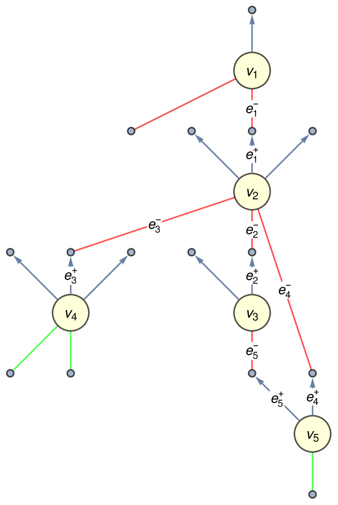
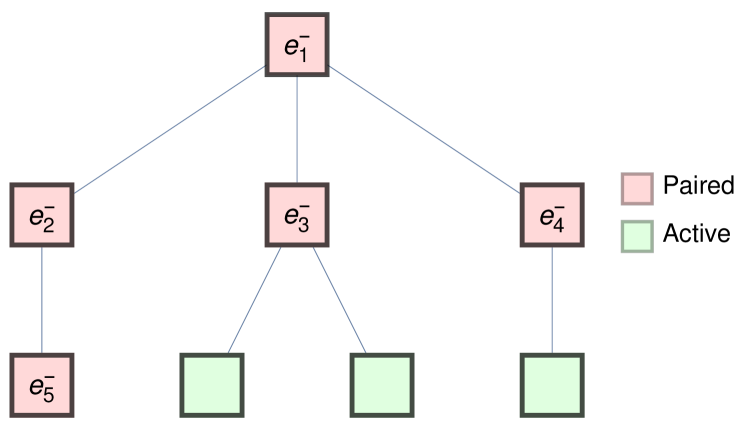
Figure 1: An ongoing exploration process and its incomplete tree

The nodes in $T^{-}_{f}(i)$ correspond to the heads in ${\cal{P}}^{-}_{i}\cup{\cal{A}}^{-}_{i}$. So we can assign a label paired or active to each node of $T^{-}_{f}(i)$. We also give the node corresponding to $e_{i}^{-}$ a mark which equals the out-degree of $v_{i}$.

For half-edges $e_{1}$ and $e_{2}$, we define the distance from $e_{1}$ to $e_{2}$, denoted by $\operatorname{dist}(e_{1},e_{2})$, to be the length of the shortest path from $v(e_{1})$ to $v(e_{2})$ which starts with the edge containing $e_{1}$ if $e_{1}$ is a tail, and which ends with the edge containing $e_{2}$ if $e_{2}$ is head. For example, in Figure 1, $\operatorname{dist}(e_{2}^{-},e_{1}^{-})=\operatorname{dist}(e_{2}^{+},e_{1}^{+})=1$, $\operatorname{dist}(e_{3}^{+},e_{1}^{-})=2$, $\operatorname{dist}(e_{4}^{-},e_{1}^{+})=0$.

If $i_{t}$ is the last step where a head at distance $t$ from $f$ is paired, then $T^{-}_{f}(i_{t})$ satisfies: (i) the height is $t$; and (ii) the set of actives nodes is the $t$-th level. We call a rooted tree $T$ incomplete if it satisfies (i)-(ii). We let $p(T)$ be the number of paired nodes in $T$.

3.2 Coupling the exploration and branching processes

We will couple a marked incomplete tree constructed from the exploration process with a marked branching process with offspring distribution close to $\eta=(\xi,\zeta)\,{\buildrel{\cal{L}}\over{=}}\,D_{{\mathrm{out}}}$. Thus we assume that $\xi\leq M$, $2\leq\zeta\leq M$ and ${\mathbb{E}}\left[\xi/\zeta\right]=1$ (by 2.2).

We will need two slightly perturbed versions of $\eta$. Let $\beta\in(0,1/4)$. Consider the probability distribution $\eta^{\downarrow}=\eta^{\downarrow}(\beta)=(\xi^{\downarrow}(\beta),\zeta^{\downarrow}(\beta))$ defined by

$${\mathbb{P}}\left\{\eta^{\downarrow}=(k,\ell)\right\}\coloneqq\begin{cases}c^{\downarrow}{\mathbb{P}}\left\{\eta=(k,\ell)\right\}&\text{if }{\mathbb{P}}\left\{\eta=(k,\ell)\right\}\geq n^{-1+\beta}\\ 0&\text{otherwise}\end{cases}$$ (3.2)

where $c^{\downarrow}$ is a normalising constant. It is easy to check that our assumptions on $\eta$ implies that $c^{\downarrow}=1+O(n^{-1+\beta})$.

Similarly, the probability distribution $\eta^{\uparrow}=\eta^{\uparrow}(\beta)$ is defined by

$${\mathbb{P}}\left\{\eta^{\uparrow}=(k,\ell)\right\}\coloneqq\begin{cases}c^{\uparrow}{\mathbb{P}}\left\{\eta=(k,\ell)\right\}&k\geq 1\\ c^{\uparrow}{\mathbb{P}}\left\{\eta=(0,\ell)\right\}+n^{-1+\beta}&k=0\end{cases}$$ (3.3)

where $c^{\uparrow}=1-O(n^{-1+\beta})$ is a normalising constant.

One can show that $\eta^{\downarrow}$ satisfies $|\mathbb{E}[\xi^{\downarrow}/\zeta^{\downarrow}]-1|=O(n^{-1+\beta})$ and similarly for $\eta^{\uparrow}$. If $\omega$ is poly-logarithmic, it will be possible to apply 2.10 to them.

Let $\mathrm{GW}_{\eta}$ be a marked Galton-Watson tree with offspring distribution $\eta$. For a marked incomplete rooted tree $T$, we use the notation $\mathrm{GW}_{\eta}\cong T$ to denote that $T$ is isomorphic to a root subtree of $\mathrm{GW}_{\eta}$, i.e., the degree of paired nodes of $T$ agrees with $\mathrm{GW}_{\eta}$, and all marks in $T$ and $\mathrm{GW}_{\eta}$ agree. For a set of incomplete trees ${\cal{T}}$, let $[\mathrm{GW}_{\eta}\in{\cal{T}}]\coloneqq\cup_{T\in{\cal{T}}}[\mathrm{GW}_{\eta}\cong T]$ and $[T^{-}_{f}\in{\cal{T}}]\coloneqq\cup_{T\in{\cal{T}}}[T^{-}_{f}(p(T))=T]$. The following is a simple adaption of [9, Lemma 5.3]; we omit the proof.

Lemma 3.1.

Let $\beta\in(0,1/4)$ and let ${\cal{T}}$ be a set of incomplete trees such that $p(T)<n^{\frac{\beta}{10}}$ for all $T\in{\cal{T}}$. We have

$$\left(1+o(1)\right){\mathbb{P}}\left\{\mathrm{GW}_{\eta^{\downarrow}{(\beta)}}\in{\cal{T}}\right\}\leq{\mathbb{P}}\left\{T^{-}_{f}\in{\cal{T}}\right\}\leq\left(1+o(1)\right){\mathbb{P}}\left\{\mathrm{GW}_{\eta^{\uparrow}(\beta)}\in{\cal{T}}\right\}\;.$$ (3.4)

4 Stationary distributions

We will proceed to prove 1.1 as in [11], using the results obtained in previous sections.

4.1 The largest strongly connected component

For $\delta^{+}\geq 2$, whp there is a linear size scc in $\vec{{\mathbb{G}}}_{n}$ [8, 14]. We will first show that whp this component is attractive (and so unique), which implies that the simple random walk on $\vec{{\mathbb{G}}}_{n}$ has a unique stationary distribution whp.

For a tail/head $e^{\pm}\in{\cal{E}}^{\pm}$, let ${\cal{N}}^{\pm}_{k}(e^{\pm})$ and ${\cal{N}}^{\pm}_{\leq k}(e^{\pm})$ be the sets of tails/heads at distance $k$ and at most $k$ from/to $e^{\pm}$, respectively; that is,

$${\cal{N}}^{+}_{k}(e^{+}) \coloneqq\left\{f^{+}\in{\cal{E}}^{+}:\operatorname{dist}(e^{+},f^{+})=k\right\}\;,\qquad {\cal{N}}^{-}_{k}(e^{-})\coloneqq\left\{f^{-}\in{\cal{E}}^{-}:\operatorname{dist}(f^{-},e^{-})=k\right\}\;,$$ (4.1)

$${\cal{N}}^{+}_{\leq k}(e^{+}) \coloneqq\left\{f^{+}\in{\cal{E}}^{+}:\operatorname{dist}(e^{+},f^{+})\leq k\right\}\;,\qquad {\cal{N}}^{-}_{\leq k}(e^{-})\coloneqq\left\{f^{-}\in{\cal{E}}^{-}:\operatorname{dist}(f^{-},e^{-})\leq k\right\}\;.$$

Similarly, for a vertex $x\in[n]$, let ${\cal{N}}^{\pm}_{k}(x)$ and ${\cal{N}}^{\pm}_{\leq k}(x)$ be the sets of vertices at distance $k$ and at most $k$ from/to $x$, respectively.

Throughout this section, let $\omega\coloneqq\log^{6}n$. For every tail/head $e^{\pm}\in{\cal{E}}^{\pm}$, consider the stopping time

$$t_{\omega}^{\pm}(e^{\pm})\coloneqq\inf\{t\geq 0:\,\absolutevalue{{\cal{N}}^{\pm}_{t}(e^{\pm})}\geq\omega\}\;;$$ (4.2)

that is, the first time when there are at least $\omega$ half-edges in the in/out-edge neighbourhood of $e^{\pm}$.

Proposition 4.1.

Let $M\in\mathbb{N}$ and suppose that $\delta^{+}\geq 2$ and $\Delta^{\pm}\leq M$. Let ${\cal{C}}_{0}$ denote the largest strongly connected component in $\vec{{\mathbb{G}}}_{n}$. Let

$${\cal{E}}^{-}_{0}\coloneqq\{f\in{\cal{E}}^{-}:t^{-}_{\omega}(f)<\infty\}\;.$$ (4.3)

Let $E_{0}$ be the event that ${\cal{C}}_{0}$ is attractive (i.e., there is a directed path from every vertex to ${\cal{C}}_{0}$) and has vertex set ${\cal{V}}_{0}={\cal{V}}({\cal{E}}_{0}^{-})$. Then ${\mathbb{P}}\left\{E_{0}\right\}=1-o(1)$. Thus, whp the simple random walk on $\vec{{\mathbb{G}}}_{n}$ has a unique stationary distribution supported on ${\cal{V}}_{0}$.

Proof.

Let $h\coloneqq 1+\log_{2}(2\omega)=O(\log\log n)$. Then, it follows from [11, Lemma 2.2] that

$${\mathbb{P}}\left\{\cup_{e\in{\cal{E}}^{+}}[t_{\omega}^{+}(e)>h]\right\} \leq{\mathbb{P}}\left\{\cup_{y\in[n]}\left[|{\cal{N}}^{+}_{h-1}(y)|\leq\omega\right]\right\}$$ (4.4)

$$\leq{\mathbb{P}}\left\{\cup_{y\in[n]}\left[|{\cal{N}}^{+}_{h-1}(y)|\leq\frac{1}{2}(\delta^{+})^{h-1}\right]\right\}=o(n^{-1})\;,$$

where we used $|{\cal{N}}^{+}_{h}(e)|\geq|{\cal{N}}^{+}_{h-1}(y)|$, where $y$ is the vertex incident to the head paired with $e$. So, $t^{+}_{\omega}(e)\leq h$ for all $e\in{\cal{E}}^{+}$ whp.

By [9, Lemma 6.2], whp every $f\in{\cal{E}}^{-}$ either has $t_{\omega}^{-}(f)=\infty$ or $t_{\omega}^{-}(f)=O(\log n)$. Conditioning on $t_{\omega}^{+}(e)=O(\log\log n)$ and $t_{\omega}^{-}(f)=O(\log n)$, [9, Proposition 7.2] implies that there is a path from $e$ to $f$ with probability $1-o(n^{-2})$. Thus, by a union bound over all choices of $e$ and $f$, we have that whp there is path from every $e\in{\cal{E}}^{+}$ to every $f\in{\cal{E}}_{0}^{-}$; and in particular, from every $x\in[n]$ to every $y\in{\cal{V}}_{0}$. In other words, whp ${\cal{C}}_{0}$ contains all vertices in ${\cal{V}}_{0}$ and is attractive. Using [9, Proposition 6.1] with $t=n/\omega$, it is easy to check that whp for every $x\in[n]\setminus{\cal{V}}_{0}$, there exists $y_{x}$ such that $y_{x}$ cannot be reached from $x$. It follows that whp ${\cal{C}}_{0}$ has vertex set ${\cal{V}}_{0}$. ∎

4.2 Random walk on heads

It will be more convenient to perform a random walk on heads instead of vertices. Consider the random process $({Z}_{t}^{{\mathbf{e}}})_{t\geq 0}$ with state space ${\cal{E}}^{-}$ and, conditioning on $\vec{{\mathbb{G}}}_{n}$ and $Z_{t}^{{\mathbf{e}}}=f$, let $Z_{t+1}^{{\mathbf{e}}}$ be chosen uniformly at random among all heads paired with tails of $v(f)$, the endpoint of $f$. It follows from 4.1 that $({Z}_{t}^{{\mathbf{e}}})_{t\geq 0}$ has a unique stationary distribution supported on ${\cal{E}}^{-}_{0}$, denoted by $\pi^{{\mathbf{e}}}$.

Recall that $\pi_{{\min}}\coloneqq\min\{\pi(y):\,y\in[n],\pi(y)>0\}$. Let $\pi_{{\min}}^{{\mathbf{e}}}\coloneqq\min\{\pi^{{\mathbf{e}}}(f):\,f\in{\cal{E}}^{-},\pi^{{\mathbf{e}}}(f)>0\}$. Define

$$\pi_{0}\coloneqq\min\{\pi(y):\,y\in{\cal{V}}_{0}\}\;,\qquad\pi_{0}^{{\mathbf{e}}}\coloneqq\min\{\pi^{{\mathbf{e}}}(f):\,f\in{\cal{E}}_{0}^{-}\}\;.$$ (4.5)

By 4.1, whp $\pi_{0}=\pi_{{\min}}$ and $\pi_{0}^{{\mathbf{e}}}=\pi_{{\min}}^{{\mathbf{e}}}$. The following lemma shows that whp $\pi_{0}^{{\mathbf{e}}}$ differs from $\pi_{0}$ by a bounded factor. Thus, it suffices to prove 1.1 for $\pi_{0}^{{\mathbf{e}}}$.

Lemma 4.2.

Whp $\pi_{0}^{{\mathbf{e}}}\leq\pi_{0}\leq M\pi_{0}^{{\mathbf{e}}}$.

Proof.

Let ${\cal{V}}_{0}$ and ${\cal{E}}_{0}^{-}$ and $E_{0}$ be as in 4.1. Since $E_{0}$ happens whp, it suffices to prove the lemma conditioning on $\vec{{\mathbb{G}}}_{n}\in E_{0}$. So we may assume there is a unique stationary distribution $\pi$ and $\lim_{t\to\infty}{\mathbb{P}}\left\{Z_{t}=y\;\middle|\;Z_{0}=x\right\}=\pi(y)$, uniformly for all $x\in[n]$.

Let $x,y\in[n]$ and $e\in{\cal{E}}^{-}(x)$. Note that $(v(Z_{t}^{{\mathbf{e}}}))_{t\geq 0}$ (i.e., the endpoints of the heads in $({Z}_{t}^{{\mathbf{e}}})_{t\geq 0}$) is itself a simple random walk on $[n]$ with the same law as $(Z_{t})_{t\geq 0}$. Therefore,

$${\mathbb{P}}\left\{Z_{t}=y\;\middle|\;Z_{0}=x\right\}=\sum_{f\in{\cal{E}}^{-}(y)}{\mathbb{P}}\left\{Z_{t}^{{\mathbf{e}}}=f\;\middle|\;Z_{0}^{{\mathbf{e}}}=e\right\}\;.$$ (4.6)

If $y\in{\cal{V}}_{0}$, then letting $t\to\infty$ on both sides we have

$$\pi(y)=\sum_{f\in{\cal{E}}^{-}(y)}\pi^{{\mathbf{e}}}(f)\geq\pi_{0}^{{\mathbf{e}}}\;,$$ (4.7)

where the last inequality holds by definition of ${\cal{V}}_{0}$. Since $y\in{\cal{V}}_{0}$ is arbitrary, it follows that $\pi_{0}\geq\pi_{0}^{{\mathbf{e}}}$.

For the other direction, let $f_{0}\in{\cal{E}}_{0}^{-}$ with $\pi^{{\mathbf{e}}}(f_{0})=\pi_{0}^{{\mathbf{e}}}$. Let $z$ be the vertex that has a tail paired with $f_{0}$. Let $e\in{\cal{E}}^{-}$ and let $x$ be its endpoint. We have

$${\mathbb{P}}\left\{Z_{t}^{{\mathbf{e}}}=f_{0}\;\middle|\;Z_{0}^{{\mathbf{e}}}=e\right\}=\frac{1}{d^{+}_{z}}{\mathbb{P}}\left\{Z_{t-1}=z\;\middle|\;Z_{0}=x\right\}\;.$$ (4.8)

Again, letting $t\to\infty$ we have

$$\pi_{0}^{{\mathbf{e}}}=\pi^{{\mathbf{e}}}(f)=\frac{1}{d^{+}_{z}}\pi(z)\geq\frac{1}{M}\pi_{0}\;.$$ (4.9)

Thus $\pi_{0}\leq M\pi_{0}^{{\mathbf{e}}}$. ∎

4.3 Lower bound for $\pi_{0}^{{\mathbf{e}}}$

To prove a lower bound it will suffice to lower bound the probability of reaching a particular head $f\in{\cal{E}}^{-}_{0}$, uniformly for all starting points $e\in{\cal{E}}^{-}$ (see 4.4 below). We use the ideas introduced in [5, 6, 11] to capture the weight (defined below) of typical trajectories departing from $e$. Our main contribution is to control the total weight of the trajectories landing at $f$.

Define the out-entropy $H^{+}$ and the entropic time $\tau_{\mathrm{\,ent}}$ as

$$H^{+}\coloneqq\frac{1}{m}\sum_{x\in[n]}d_{x}^{-}\log d_{x}^{+},\quad\tau_{\mathrm{\,ent}}\coloneqq\frac{\log n}{H^{+}}\;.$$ (4.10)

We stress the similarity between $H^{+}$ and $\hat{H}^{-}$ defined in (1.8); in particular, $H^{+}=\mathbb{E}[\log D_{{\mathrm{in}}}^{+}]$. In this case, the out-entropy is related to typical trajectories in supercritical out-growth.

Fix $\varepsilon>0$ small enough and let

$$h^{+}\coloneqq(1-\varepsilon)\tau_{\mathrm{\,ent}},\qquad h^{-}\coloneqq\frac{3\varepsilon}{\log\delta^{+}}\log n\;.$$ (4.11)

For $f\in{\cal{E}}^{-}$, let $h(f)\coloneqq t^{-}_{\omega}(f)\wedge\omega$. Define

$$\tau(f)\coloneqq h^{+}+h^{-}+h(f)\;.$$ (4.12)

Remark 4.3.

Bordenave, Caputo and Salez [5, 6] showed that the mixing time of the random walk on $\vec{{\mathbb{G}}}_{n}$ coincides with the entropic time, and exhibits cutoff. Jensen’s inequality implies that $\tau_{\mathrm{\,ent}}\geq(1+o(1))\log_{\nu}n$, which is whp the typical distance of the $\vec{{\mathbb{G}}}_{n}$. Thus, by the results in [9], $\tau_{\mathrm{\,ent}}+\max_{f\in{\cal{E}}^{-}_{0}}h(f)$ is at least the diameter of $\vec{{\mathbb{G}}}_{n}$ whp.

Throughout this section, we will use letters $a,b$ for tails in ${\cal{E}}^{+}$ and letters $e,f,g$ for heads in ${\cal{E}}^{-}$. Let $P^{t}(e,f)\coloneqq{\mathbb{P}}\left\{Z^{{\mathbf{e}}}_{t}=f\;\middle|\;Z^{{\mathbf{e}}}_{0}=e\right\}$. To lower bound $\pi_{0}^{\mathbf{e}}$ it suffices to prove the following:

Lemma 4.4.

With high probability, for all $e\in{\cal{E}}^{-}$ and $f\in{\cal{E}}_{0}^{-}$,

$$P^{\tau(f)}(e,f)\geq n^{-(1+\hat{H}^{-}/\phi(a_{0})+o(1))}\;.$$ (4.13)

Let $f\in{\cal{E}}^{-}_{0}$. Assuming 4.4 and by stationarity at time $\tau(f)$, whp we have

$$\pi^{{\mathbf{e}}}(f)=\sum_{e\in{\cal{E}}^{-}}\pi^{\mathbf{e}}(e)P^{\tau({f})}(e,f)\geq n^{-(1+\hat{H}^{-}/\phi(a_{0})+o(1))}\;,$$ (4.14)

and the lower bound in 1.1 follows.

From now on, we fix two heads $e,f\in{\cal{E}}^{-}$. We sequentially expose the out-neighbourhood of $e$ (out-phase) and the in-neighbourhood of $f$ (in-phase) as explained below. To control the trajectories departing from $e$, we will use the idea of nice paths introduced in [5] as described in [11].

In the out-phase we build a directed rooted tree $T^{+}_{e}$, partially exposing the out-neighbourhood of $e$. The root of $T^{+}_{e}$ represents the head $e$ and all its other nodes represent tails in ${\cal{E}}^{+}$. For a tail $a$ represented in $T^{+}_{e}$, let ${\mathbf{h}}(a)$ denote its height in $T^{+}_{e}$. Define its weight by

$${\mathbf{w}}(a)\coloneqq\prod_{i=1}^{{\mathbf{h}}(a)}\frac{1}{d^{+}_{v(a_{i})}}\;.$$ (4.15)

where $a_{1},\dots,a_{{\mathbf{h}}(a)}$ are the tails in the path from $e$ to $a$ in $T^{+}_{e}$.

To construct $T^{+}_{e}$ we use a procedure similar to Subsection 3.1, with the roles of heads and tails reversed and the following two modifications:

1. There is no initial tail $e_{0}^{+}$. We start at step $i=2$ with $e_{1}^{-}=e$ and ${\cal{A}}_{1}^{\pm}={\cal{E}}^{\pm}(v(e))$.

2. For each $i\geq 2$, at step (i) we choose $e^{+}_{i}$ to be the tail in ${\cal{A}}_{i-1}^{+}$ that maximises ${\mathbf{w}}(a)$ among all $a\in{\cal{A}}_{i-1}^{+}$ with ${\mathbf{h}}(a)\leq h^{+}-1$ and ${\mathbf{w}}(a)\geq n^{-1+\varepsilon^{2}}$.

The tree $T_{e}^{+}$ is not constructed in a BFS manner, but maximising the weight of its nodes; by construction, ${\mathbf{h}}(a)\geq\operatorname{dist}(e,a)+1$. The process stops if there are no more eligible tails. In [6, Lemma 7], the authors showed that deterministically constructing $T^{+}_{e}$ exposes at most $\kappa^{+}\coloneqq n^{1-\varepsilon^{2}/2}$ edges. Moreover, if $g$ is the head paired with a tail $a$ represented in $T_{e}^{+}$, we have $P^{{\mathbf{h}}(a)}(e,g)\geq{\mathbf{w}}(a)$.

In the in-phase we build a directed rooted tree $T_{f}^{-}$, exposing ${\cal{N}}^{-}_{\leq h^{-}+h(f)}(f)$ conditionally on $T^{+}_{e}$. We use the exploration process defined in Subsection 3.1 with one modification: if $e^{-}_{i}$ has already been paired with $e^{+}$ in the exploration of $T^{+}_{e}$, we let $e^{+}_{i}=e^{+}$. We stop once all heads at distance $h^{-}+h(f)$ from $f$ have been activated and we let $T_{f}^{-}$ be the final incomplete tree generated up to this point. For a head $g$ in $T^{-}_{f}$, let ${\mathbf{h}}(g)$ be its height in $T^{-}_{f}$; note that ${\mathbf{h}}(g)=\operatorname{dist}(g,f)$. We define its weight by

$${\mathbf{w}}(g)\coloneqq\prod_{i=1}^{{\mathbf{h}}(g)}\frac{1}{d^{+}_{v(g_{i})}}\;,$$ (4.16)

where $f=g_{0},\dots,g_{{\mathbf{h}}(g)}$ are the heads in the path from $f$ to $g$ in $T^{-}_{f}$. Similarly as before, $P^{{\mathbf{h}}(g)}(g,f)\geq{\mathbf{w}}(g)$. For any $\alpha>0$, we can let $\varepsilon$ be small enough such that the number of edges exposed in the in-phase is at most

$$\kappa^{-}\coloneqq\omega h(f)+\omega(\Delta^{-})^{h^{-}+1}=n^{3(\log{\Delta^{-}}/\log\delta^{+})\varepsilon+o(1)}=O(n^{\alpha})\;.$$ (4.17)

Let $\sigma_{0}$ be a partial realisation of the configuration model in which at most $\kappa\coloneqq\kappa^{+}+\kappa^{-}$ edges are revealed during the out- and in-phases. Then $T_{e}^{+},T_{f}^{-}$, $h(f)$, ${\cal{N}}^{-}_{\leq h^{-}+h(f)}(f)$ and $\tau(f)$ are all measurable with respect to $\sigma_{0}$. Given $\sigma_{0}$, let ${\cal{A}}$ be the set of unpaired tails $a$ in $T_{e}^{+}$ with ${\mathbf{h}}(a)=h^{+}$, and let ${\cal{G}}$ be the set of unpaired heads $g$ in $T_{f}^{-}$ which satisfy ${\mathbf{h}}(g)=h^{-}+h(y)$.

To bound the desired probability, it will be convenient to consider trajectories that are not too heavy. Following the ideas in [5, 6, 11], it suffices to only consider nice paths in $T_{f}^{-}$; that is, we restrict our attention to the tails $a\in{\cal{A}}$ such that $\mathbf{w}(a)\leq n^{-1+2\epsilon}$. For heads in ${\cal{G}}$, we define a truncated version of the weight. Let $\gamma\coloneqq n^{-{(1+\varepsilon)\hat{H}^{-}}/{\phi(a_{0})}}$. For $g$ in $T_{f}^{-}$ with ${\mathbf{h}}(g)\geq h(f)$, we define its truncated weight by

$$\hat{{\mathbf{w}}}(g)\coloneqq({\mathbf{w}}(\hat{g})\wedge\gamma)\prod_{i=h(f)+1}^{{\mathbf{h}}(g)}\frac{1}{d^{+}_{v(g_{i})}}\;.$$ (4.18)

where $\hat{g}$ is the unique head in the path from $f$ to $g$ in $T_{f}^{-}$ with ${\mathbf{h}}(\hat{g})=h(f)$. In words, the truncated weight caps the contribution of the last $h(f)$ steps by $\gamma$. By the definition of $h^{-}$ in (4.11), for $g\in{\cal{G}}$ we have

$$\hat{{\mathbf{w}}}(g) \leq(\delta^{+})^{-h^{-}}\gamma\leq\gamma n^{-3\varepsilon}\;.$$ (4.19)

Let $\sigma$ be a complete pairing of half-edges compatible with $\sigma_{0}$. Let $[\sigma(a)=g]$ be the event that $a$ and $g$ are paired in $\sigma$. Conditioning on $\sigma_{0}$, we can lower bound the desired probability as follows

$$P^{\tau(f)}(e,f)\geq\hat{P}^{\tau(f)}(e,f)\coloneqq\sum_{a\in{\cal{A}}}\sum_{g\in{\cal{G}}}{\mathbf{w}}(a)\mathbf{\hat{w}}(g)\mathbf{1}_{\sigma(a)=g}\mathbf{1}_{{\mathbf{w}}(a)\leq n^{-1+2\varepsilon}}\;.$$ (4.20)

Let

$$A_{e,f}(\sigma_{0})\coloneqq\sum_{a\in{\cal{A}}}{\mathbf{w}}(a)\mathbf{1}_{{\mathbf{w}}(a)\leq n^{-1+2\varepsilon}}\;,\qquad B_{e,f}(\sigma_{0})\coloneqq\sum_{g\in{\cal{G}}}\mathbf{\hat{w}}(g)\;,\qquad$$ (4.21)

which are measurable with respect to $\sigma_{0}$. Consider the event

$${\cal{Y}}_{e,f}=\left\{\sigma_{0}:\,A_{e,f}(\sigma_{0})\geq\frac{1}{2},\;B_{e,f}(\sigma_{0})\geq\frac{\omega\gamma}{4}\;\right\}\;.$$ (4.22)

If $\sigma_{0}\in{\cal{Y}}_{e,f}$, then

$${\mathbb{E}}\left[\hat{P}^{\tau(f)}(e,f)\;\middle|\;\sigma_{0}\right]\geq\frac{1}{m}A_{e,f}(\sigma_{0})B_{e,f}(\sigma_{0})\geq\frac{\omega\gamma}{8m}\geq\frac{2\gamma}{n}\;.$$ (4.23)

We prove a concentration result similar to [11, Lemma 3.6], exploiting the truncated nature of $\hat{P}^{t}$:

Lemma 4.5.

For every $\sigma_{0}\in{\cal{Y}}_{e,f}$ and every $a\in(0,1)$

$${\mathbb{P}}\left\{\hat{P}^{\tau(f)}(e,f)\leq(1-a){\mathbb{E}}\left[\hat{P}^{\tau(f)}(e,f)\;\middle|\;\sigma_{0}\right]\;\middle|\;\sigma_{0}\right\}\leq\exp(-\frac{a^{2}n^{\varepsilon}}{3})\;.$$

Proof.

One can write $\hat{P}^{\tau(f)}(e,f)=\sum_{a\in{\cal{E}}^{+}}c(a,\sigma(a))$ where

$$c(a,g)={\mathbf{w}}(a)\hat{{\mathbf{w}}}(g)\mathbf{1}_{{\mathbf{w}}(a)\leq n^{2\varepsilon-1}}\mathbf{1}_{a\in{\cal{A}},g\in{\cal{G}}}\;.$$ (4.24)

By (4.19), it follows that

$$\|c\|_{\infty}\coloneqq\max_{a\in{\cal{E}}^{+}}c(a,\sigma(a))\leq\gamma n^{-(1+\varepsilon)}\;.$$ (4.25)

Using the one-sided version of Chatterjee’s inequality for uniformly random pairings [12, Proposition 1.1], we get that

$${\mathbb{P}}\left\{\hat{P}^{\tau(f)}(e,f)\leq(1-a){\mathbb{E}}\left[\hat{P}^{\tau(f)}(e,f)\;\middle|\;\sigma_{0}\right]\;\middle|\;\sigma_{0}\right\}\leq\exp(-\frac{a^{2}{\mathbb{E}}\left[\hat{P}^{\tau(f)}(e,f)\;\middle|\;\sigma_{0}\right]}{6\|c\|_{\infty}})\leq e^{-\frac{a^{2}n^{\varepsilon}}{3}}\;,$$

where we used (4.23) in the last line. ∎

Lemma 4.6.

Define the event

$${\cal{Y}}=\bigcap_{e,f\in{\cal{E}}^{-}}({\cal{Y}}_{e,f}\cup[t^{-}_{\omega}(f)=\infty])\;.$$ (4.26)

We have ${\mathbb{P}}\left\{{\cal{Y}}\right\}=1-o(1).$

Let us prove 4.4 assuming that 4.6 holds. The proof of 4.6 is postponed to Subsection 4.4.

Proof of 4.4.

Write

$$E_{f}\coloneqq[t_{\omega}^{-}(f)=\infty]\;,\qquad F_{e,f}\coloneqq\left[\hat{P}^{\tau(f)}(e,f)\geq\frac{\gamma}{n}\right]\;.$$ (4.27)

Using (4.23) and applying 4.5 with $a=1/3$,

$${\mathbb{P}}\left\{F_{e,f}^{c}\;\middle|\;{\cal{Y}}_{e,f}\right\}={\mathbb{P}}\left\{\hat{P}^{\tau(f)}(e,f)<\frac{\gamma}{n}\;\middle|\;{\cal{Y}}_{e,f}\right\}\leq\max_{\sigma_{0}\in{\cal{Y}}_{e,f}}{\mathbb{P}}\left\{\hat{P}^{\tau(f)}(e,f)<\frac{\gamma}{n}\;\middle|\;\sigma_{0}\right\}=o(n^{-2})\;.$$ (4.28)

It follows that,

$${\mathbb{P}}\left\{\cap_{e,f\in{\cal{E}}^{-}}(F_{e,f}\cup E_{f})\right\} \geq{\mathbb{P}}\left\{{\cal{Y}}\cap(\cap_{e,f\in{\cal{E}}^{-}}(F_{e,f}\cup E_{f}))\right\}$$

$$={\mathbb{P}}\left\{{\cal{Y}}\right\}-{\mathbb{P}}\left\{{\cal{Y}}\cap\left(\cap_{e,f\in{\cal{E}}^{-}}(F_{e,f}\cup E_{f})\right)^{c}\right\}$$

$$\geq(1-o(1))-\sum_{e,f\in{\cal{E}}^{-}}{\mathbb{P}}\left\{{\cal{Y}}\cap F_{e,f}^{c}\cap E_{f}^{c}\right\}$$

$$\geq(1-o(1))-\sum_{e,f\in{\cal{E}}^{-}}{\mathbb{P}}\left\{F_{e,f}^{c}\cap{\cal{Y}}_{e,f}\right\}$$

$$\geq(1-o(1))-\sum_{e,f\in{\cal{E}}^{-}}{\mathbb{P}}\left\{F_{e,f}^{c}\mid{\cal{Y}}_{e,f}\right\}$$

$$=1-o(1)\;,$$

where we used that ${\cal{Y}}\cap E_{f}^{c}$ implies ${\cal{Y}}_{e,f}$.

So, whp, if $t^{-}_{\omega}(f)<\infty$, then $F_{e,f}$ holds. In other words, we have shown that for all $e\in{\cal{E}}^{-}$ and $f\in{\cal{E}}_{0}^{-}$,

$$P^{\tau(f)}(e,f)\geq\hat{P}^{\tau(f)}(e,f)\geq\frac{\gamma}{n}\geq n^{-(1+(1+\epsilon)\hat{H}^{-}/\phi(a_{0}))}.$$ (4.29)

Since $\varepsilon$ can be arbitrarily small, this proves the lemma. ∎

4.4 Proof of 4.6

Define the following events

$${\cal{A}}_{1}=\bigcap_{e,f\in{\cal{E}}^{-}}\left[A_{e,f}\geq\frac{1}{2}\right]\;,\qquad{\cal{A}}_{2}=\bigcap_{e,f\in{\cal{E}}^{-}}\left[B_{e,f}\geq\frac{\omega\gamma}{4}\right]\cup[t^{-}_{\omega}(f)=\infty]\;,$$ (4.30)

and note that ${\cal{Y}}\supseteq{\cal{A}}_{1}\cap{\cal{A}}_{2}$.

The vertex analogue of the event ${\cal{A}}_{1}$ was studied in [11, Lemma 3.7]. Note that its proof does not use any assumption on $\delta^{-}$, is valid for tail-trees instead of vertex-trees and accommodates the $\kappa^{-}=O(n^{\alpha})$ half-edges revealed during the in-phase. Thus the conclusion ${\mathbb{P}}\left\{{\cal{A}}_{1}\right\}=1-o(1)$ still holds in our setting.

We are left with showing the following lemma:

Lemma 4.7.

We have ${\mathbb{P}}\left\{{\cal{A}}_{2}\right\}=1-o(1)$.

Proof.

In order to analyse the probability of ${\cal{A}}_{2}$, it will be convenient to swap the order of the phases: we first run the in-phase unconditionally, and then the out-phase. Write $h=h(f)+h^{-}$. We will first prove that

$$\hat{\Gamma}^{\mathbf{T}}_{h}(f)\coloneqq\sum_{g\in{\cal{N}}^{-}_{h}(f)}\hat{{\mathbf{w}}}(g)\;,$$ (4.31)

is large using branching processes. Note that the difference between $\hat{\Gamma}^{\mathbf{T}}_{h}(f)$ and $B_{e,f}$ (defined in (4.21)) is that the latter does not include the weight of heads that are paired in the out-phase.

Consider the marked branching process $X_{t}$ with offspring distribution $\eta^{\uparrow}=\eta^{\uparrow}(\beta)$, where $\eta=D_{{\mathrm{out}}}$ and $\beta<1/4$ will be fixed later. We define $\hat{\nu}^{\uparrow}$, $\hat{H}^{\uparrow}$, $\phi^{\uparrow}(a)$, $a_{0}^{\uparrow}$ for $\eta^{\uparrow}$ analogously to $\hat{\nu}$, $\hat{H}$, $\phi(a)$ and $a_{0}$ for $\eta$ (see (2.8), (2.13) and (2.58)). It is easy to verify that $\hat{\nu}^{\uparrow}=(1+o(1))\hat{\nu}$, $\hat{H}^{\uparrow}=(1+o(1))\hat{H}$ and $\phi^{\uparrow}(a)=(1+o(1))\phi(a)$. By continuity of $\phi(a)$, we have $\phi^{\uparrow}(a_{0}^{\uparrow})=(1+o(1))\phi(a_{0})$. So $\hat{H}^{\uparrow}/\phi^{\uparrow}(a_{0}^{\uparrow})=(1+o(1))\hat{H}/\phi(a_{0})$. Define $\gamma^{\uparrow}\coloneqq n^{-{(1+\varepsilon/2)\hat{H}^{\uparrow}}/{\phi^{\uparrow}(a_{0}^{\uparrow})}}>\gamma$.

Let $E_{1}(f)\coloneqq[\hat{\Gamma}^{\mathbf{T}}_{h}(f)<\omega\gamma/2]$ and $E_{2}(f)\coloneqq[t^{-}_{\omega}(f)<\omega]$. Recall the definition of $\hat{\Gamma}_{t}$ in (2.63) and let $E_{1}\coloneqq[\hat{\Gamma}_{t_{\omega}+h^{-}}<\omega\gamma/2]$ and $E_{2}\coloneqq[t_{\omega}<\omega]$. Let $E_{1}^{\uparrow}\coloneqq[\hat{\Gamma}_{t_{\omega}+h^{-}}<\omega\gamma^{\uparrow}/2]$ and note that $E_{1}\subseteq E_{1}^{\uparrow}$.

2.9 with $p=n^{-(1+\varepsilon/2)}$ shows that

$${\mathbb{P}}\left\{(G_{t_{\omega}}(\gamma^{\uparrow}))^{c}\cap E_{2}\right\}\leq{\mathbb{P}}\left\{(G_{t_{\omega}}(\gamma^{\uparrow}))^{c}\cap[t_{\omega}<\infty]\right\}=O(n^{-(1+\varepsilon/4)})\;.$$ (4.32)

So using 2.10

$${\mathbb{P}}\left\{E_{1}^{\uparrow}\cap E_{2}\right\} \leq{\mathbb{P}}\left\{E_{1}^{\uparrow}\cap E_{2}\cap G_{t_{\omega}}(\gamma^{\uparrow})\right\}+{\mathbb{P}}\left\{(G_{t_{\omega}}(\gamma^{\uparrow}))^{c}\cap E_{2}\right\}$$ (4.33)

$$\leq\sum_{t_{0}=1}^{\omega}\mathbb{P}\left\{E_{1}^{\uparrow}\;\middle|\;[t_{\omega}=t_{0}]\cap G_{t_{0}}(\gamma)\right\}\mathbb{P}\left\{t_{\omega}=t_{0}\;\middle|\;t_{\omega}<\omega\right\}+O(n^{-(1+\varepsilon/4)})$$

$$=e^{-c_{0}\omega^{1/3}}+O(n^{-(1+\varepsilon/4)})=O(n^{-(1+\varepsilon/4)})\;.$$

Let $T$ be a marked incomplete tree of height $\omega+h^{-}\geq h$. Recall that $p(T)$ is the number of paired nodes in $T$ and that $T^{-}_{f}(i)$ is the marked incomplete tree constructed after the $i$-th pairing in the graph exploration process. Conditional on $[T^{-}_{f}(p(T))=T]$, the events $E_{1}(f)$ and $E_{2}(f)$ are measurable. Let ${\cal{T}}$ be the set of incomplete trees $T$ of height $\omega+h^{-}$ that satisfy $E_{1}(f)\cap E_{2}(f)$. Note that $p(T)\leq\kappa^{-}=O(n^{\alpha})$ for a constant $\alpha>0$ as small as needed. Thus, by 3.1 with $\beta=10\alpha$ and (4.33), we have

$${\mathbb{P}}\left\{E_{1}(f)\cap E_{2}(f)\right\} ={\mathbb{P}}\left\{T_{f}^{-}\in{\cal{T}}\right\}$$ (4.34)

$$\leq(1+o(1)){\mathbb{P}}\left\{\mathrm{GW}_{\eta^{\uparrow}}\in{\cal{T}}\right\}$$

$$=(1+o(1)){\mathbb{P}}\left\{E_{1}\cap E_{2}\right\}$$

$$\leq(1+o(1)){\mathbb{P}}\left\{E_{1}^{\uparrow}\cap E_{2}\right\}$$

$$=O(n^{-(1+\varepsilon/4)})\;.$$

By 2.7, we have ${\mathbb{P}}\left\{E_{2}^{c}\;\middle|\;t_{\omega}<\infty\right\}=o(n^{-2})$. Applying 3.1 similarly as before shows that ${\mathbb{P}}\left\{(E_{2}(f))^{c}\;\middle|\;t_{\omega}^{-}(f)<\infty\right\}=o(n^{-2})$. Therefore, it follows from (4.34) that

$${\mathbb{P}}\left\{[\hat{\Gamma}^{\mathbf{T}}_{h}(f)\geq\omega\gamma/2]\cup[t_{\omega}^{-}(f)=\infty]\right\}=1-O(n^{-(1+\varepsilon/2)})\;.$$ (4.35)

Thus, by applying the union bound first over $f\in{\cal{E}}^{-}$ and then over $e\in{\cal{E}}^{-}$, we have

$${\mathbb{P}}\left\{{\cal{A}}^{c}_{2}\right\}=o(1)+\sum_{e,f\in{\cal{E}}^{-}}{\mathbb{P}}\left\{\left[B_{e,f}<\frac{\omega\gamma}{4}\right]\cap\left[\hat{\Gamma}^{\mathbf{T}}_{h}(f)\geq\frac{\omega\gamma}{2}\right]\right\}\;.$$ (4.36)

Let $\sigma^{-}$ be a partial pairing of the at most $\kappa^{-}=o(n)$ half-edges that expose ${\cal{N}}_{\leq h}^{-}(f)$. We now perform the out-phase to construct the tree $T^{+}_{e}$ conditional on $\sigma^{-}$. Recall that during the out-phase at most $\kappa^{+}=o(n)$ edges are formed. Thus,

$${\mathbb{E}}\left[B_{e,f}\;\middle|\;\sigma^{-}\right] =\sum_{g\in{\cal{N}}^{-}_{h}(f)}\hat{{\mathbf{w}}}(g){\mathbb{E}}\left[\mathbf{1}_{g\in{\cal{G}}}\;\middle|\;\sigma^{-}\right]$$ (4.37)

$$\geq\left(1-\frac{\kappa^{+}}{m-\kappa^{+}-\kappa^{-}}\right)\sum_{g\in{\cal{N}}^{-}_{h}(f)}\hat{{\mathbf{w}}}(g)$$

$$=(1+o(1))\hat{\Gamma}^{\mathbf{T}}_{h}(f)\;.$$

Using (4.19), an application of Azuma’s inequality (see [21, Chapter 11]) to $B_{e,f}$ determined by the random vector $\left(\hat{{\mathbf{w}}}(g)\mathbf{1}_{g\in{\cal{G}}}\right)_{g\in{\cal{N}}^{-}_{h}(f)}$ implies that

$${\mathbb{P}}\left\{B_{e,f}<\frac{\hat{\Gamma}^{\mathbf{T}}_{h}(f)}{2}\;\middle|\;\sigma^{-}\right\}\leq\exp\left\{-2\frac{(1+o(1)\hat{\Gamma}^{\mathbf{T}}_{h}(f)^{2}}{\sum_{g\in{\cal{N}}^{-}_{h}(f)}\hat{{\mathbf{w}}}(g)^{2}}\right\}\leq\exp\left\{-2\gamma^{-1}n^{2\varepsilon}\hat{\Gamma}^{\mathbf{T}}_{h}(f)\right\}\;.$$ (4.38)

Since the event $[\hat{\Gamma}^{\mathbf{T}}_{h}(f)>\frac{\omega\gamma}{2}]$ is measurable with respect to $\sigma^{-}$, we have

$${\mathbb{P}}\left\{\left[B_{e,f}<\frac{\omega\gamma}{4}\right]\cap\left[\hat{\Gamma}^{\mathbf{T}}_{h}(f)>\frac{\omega\gamma}{2}\right]\right\}\leq\exp\left\{-2\gamma^{-1}n^{2\varepsilon}\left(\frac{\omega\gamma}{2}\right)\right\}\leq\exp\left\{-\omega n^{2\varepsilon}\right\}\;.$$ (4.39)

Putting this into (4.36) finishes the proof. ∎

4.5 Upper bound for $\pi_{0}^{{\mathbf{e}}}$

Let $\varepsilon>0$ be small enough. Let $a_{0}$ be the minimiser of $\phi(a)$, defined as in (1.10). Let

$$h_{1}\coloneqq\frac{1-\varepsilon}{a_{0}\phi(a_{0})}\log{n}\;,\qquad h_{2}\coloneqq\log_{\nu}\omega=O(\log\log n)\;.$$ (4.40)

In this subsection we set $\gamma\coloneqq n^{-{(1-\varepsilon)\hat{H}^{-}}/{\phi(a_{0})}}$. Let $\Gamma_{t}(f)$ be a graph analogue of $\Gamma_{t}$ (see Section 2) defined by

$$\Gamma_{t}(f)\coloneqq\sum_{g\in{\cal{N}}_{t}^{-}(f)}P^{t}(g,f)\;.$$ (4.41)

Recall the definition of $\mathbf{w}(g)$ in (4.16). Define

$$\Gamma^{{\mathbf{T}}}_{t}(f)\coloneqq\sum_{g\in{\cal{N}}^{-}_{t}(f)}{\mathbf{w}}(g)\;.$$ (4.42)

For any subgraph $G$ with vertex set a subset of $[n]$, let ${\text{TX}}(G)\coloneqq|E(G)|-(|V(G)|-1)$ denote the excess of edges of $G$ comparing to the case when it induces a tree.

For $f\in{\cal{E}}^{-}$, consider the following events:

$$E_{0}(f)=[t^{-}_{\omega}(f)\leq h_{1}+h_{2}]\;, E_{1}(f)=[0<\Gamma^{{\mathbf{T}}}_{h_{1}}(f)<\gamma]\;,$$ (4.43)

$$E_{2}(f)=[{\text{TX}}({\cal{N}}^{-}_{\leq h_{1}}(f))=0]\;, F(f)=\bigcap_{r=1}^{h_{1}}[0<|{\cal{N}}^{-}_{r}(f)|<\omega]\;.$$

Write ${\cal{A}}(f)=E_{0}(f)\cap E_{1}(f)\cap E_{2}(f)\cap F(f)$.

The proof in this section uses $T^{-}_{f}$, the tree constructed in Subsection 3.1, stopping once all heads at distance $h_{1}+h_{2}$ to $f$ have become active. During the construction of $T^{-}_{f}$ we deterministically expose at most $\kappa^{-}_{1}\coloneqq\omega h_{1}+\omega(\Delta^{-})^{h_{2}+1}=O(\log^{C}n)$ pairings for some constant $C$.

Proposition 4.8.

For all $f\in{\cal{E}}^{-}$, we have

$${\mathbb{P}}\left\{{\cal{A}}(f)\right\}=n^{-1+\varepsilon+o(1)}\;.$$ (4.44)

Proof.

Consider $E_{0}=[t_{\omega}\leq h_{1}+h_{2}]$, $E_{1}=[0<\Gamma_{h_{1}}<\gamma]$ and $F=\bigcap_{r=1}^{h_{1}}[0<X_{r}<\omega]$ to be the corresponding events on the marked branching process $(X_{r})_{r\geq 0}$ with offspring distribution $\eta^{\downarrow}(\beta)$ with $\eta=D_{{\mathrm{out}}}$ and an arbitrary $\beta\in(0,1/4)$ to be determined later. With $a=a_{0}$ and $t=h_{1}$, 2.5 implies that

$${\mathbb{P}}\left\{E_{1}\cap F\right\}\geq n^{-1+\varepsilon+o(1)}\;.$$ (4.45)

When $F$ happens, there is at least one individual in generation $h_{1}$. Thus, for some constant $c$,

$${\mathbb{P}}\left\{E_{0}\;\middle|\;E_{1}\cap F\right\}\geq{\mathbb{P}}\left\{X_{h_{2}+h_{1}}\geq\omega\;\middle|\;X_{h_{1}}>0\right\}\geq{\mathbb{P}}\left\{X_{h_{2}}\geq\omega\right\}>c\;,$$ (4.46)

where in the last inequality we used that $\nu^{-h}X_{h}$ converges to an absolutely continuous random variable, and $h_{2}=\log_{\nu}\omega$. Therefore, ${\mathbb{P}}\left\{E_{0}\cap E_{1}\cap F\right\}\geq n^{-1+\varepsilon+o(1)}$.

Conditional on $[T^{-}_{f}(p(T))=T]$, the event $E_{0}(f)\cap E_{1}(f)\cap F(f)$ is measurable. Let ${\cal{T}}$ be the set of incomplete trees $T$ that satisfy $E_{0}(f)\cap E_{1}(f)\cap F(f)$. Using 3.1 we have

$${\mathbb{P}}\left\{E_{0}(f)\cap E_{1}(f)\cap F(f)\right\}\geq(1+o(1)){\mathbb{P}}\left\{\mathrm{GW}_{\eta^{\downarrow}}\in{\cal{T}}\right\}\geq n^{-1+\varepsilon+o(1)}\;,$$ (4.47)

where we used that the parameters $\hat{\nu}^{\downarrow}$, $\hat{H}^{\downarrow}$, $\phi^{\downarrow}(a_{0}^{\downarrow})$ are well-approximated by $\hat{\nu}$, $\hat{H}$, $\phi(a_{0})$, as in the proof of 4.7.

We next bound the probability of $(E_{2}(f))^{c}\cap F(f)$. Recall that ${\text{TX}}({\cal{N}}_{\leq h_{1}}^{-}(f))$ is the number of collisions; that is, steps in the exploration process where $e_{i}^{+}\in{\cal{A}}^{+}_{i-1}$. At step $i$, the probability of a collision is at most $\frac{\Delta^{+}i}{m-i+1}$. So, provided $\ell\leq m/2$, the number of collisions in the first $\ell$ steps is dominated by a binomial random variable with parameters $(\ell,2\ell M/m)$. Note that the probability of $(E_{2}(f))^{c}\cap F(f)$ is bounded from above by the probability of at least one collision happens when running the exploration process for at most $\ell=(\omega-1)h_{1}=O(\log^{7}n)$ steps. Thus we have

$${\mathbb{P}}\left\{(E_{2}(f))^{c}\cap F(f)\right\}=O(\ell^{2}/m)=n^{-1+o(1)}\;.$$ (4.48)

Thus, we obtain the lower bound in (4.44):

$${\mathbb{P}}\left\{{\cal{A}}(f)\right\} ={\mathbb{P}}\left\{E_{0}(f)\cap E_{1}(f)\cap E_{2}(f)\cap F(f)\right\}$$

$$\geq{\mathbb{P}}\left\{E_{0}(f)\cap E_{1}(f)\cap F(f)\right\}-{\mathbb{P}}\left\{(E_{2}(f))^{c}\cap F(f)\right\}\geq n^{-1+\varepsilon+o(1)}\;.$$

For the upper bound in (4.44), an application of 2.6 with offspring $\eta^{\uparrow}(\beta)$, $a=a^{\uparrow}_{0}$ and $t=h_{1}$, and 3.1, as in the proof of 4.7, gives that

$$\begin{aligned} {\mathbb{P}}\left\{{\cal{A}}(f)\right\}&\leq{\mathbb{P}}\left\{E_{1}(f)\cap F(f)\right\}\\ &\leq(1+o(1)){\mathbb{P}}\left\{E_{1}\cap F\right\}\\ &\leq{\mathbb{P}}\left\{(G_{t}(e^{-a\hat{H}t}))^{c}\cap[0<X_{t}<\omega]\right\}\\ &\leq n^{-1+\varepsilon+o(1)}\;.\end{aligned}\qed$$ (4.49)

We will show that $Z\coloneqq\sum_{f\in{\cal{E}}^{-}}\mathbf{1}_{{\cal{A}}(f)}$ satisfies $Z>0$ whp, using a second moment calculation. As $m\geq n$, 4.8 implies that $\mathbb{E}[Z]\geq n^{\varepsilon/2}$. For a partial pairing $\sigma_{0}$, we write $f\in Im(\sigma_{0})$ if $f$ has been paired by $\sigma_{0}$. For $f_{1},f_{2}\in{\cal{E}}^{-}$ with $f_{1}\neq f_{2}$, we have

$${\mathbb{P}}\left\{{\cal{A}}(f_{1})\cap{\cal{A}}(f_{2})\right\} \leq\sum_{\sigma_{0}\in{\cal{A}}(f_{1})}{\mathbb{P}}\left\{\sigma_{0}\right\}\left(\mathbf{1}_{f_{2}\in Im(\sigma_{0})}+\mathbf{1}_{f_{2}\notin Im(\sigma_{0})}{\mathbb{P}}\left\{{\cal{A}}(f_{2})\mid\sigma_{0}\right\}\right)$$ (4.50)

$$\leq{\mathbb{P}}\left\{{\cal{A}}(f_{1})\right\}\left(O\left(\frac{\log^{C}n}{n}\right)+\max_{\begin{subarray}{c}\sigma_{0}\in{\cal{A}}(f_{1})\\ f_{2}\notin Im(\sigma_{0})\end{subarray}}{\mathbb{P}}\left\{{\cal{A}}(f_{2})\mid\sigma_{0}\right\}\right)\;,$$ (4.51)

where we used that at most $\kappa_{1}^{-}=O(\log^{C}n)$ edges need to be exposed to determine ${\cal{A}}(f_{1})$.

We briefly describe how to compute ${\mathbb{P}}\left\{{\cal{A}}(f_{2})\mid\sigma_{0}\right\}$ for $f_{2}\notin\imaginary(\sigma_{0})$. Start the exploration process in Subsection 3.1 from $f_{2}$ with one modification: if $e^{-}_{i}$ has already been paired in $\sigma_{0}$, then we choose $e^{+}_{i}$ according to $\sigma_{0}$ instead of uniformly at random. Since at most $\kappa_{1}^{-}$ half-edges need to be paired, the probability of $[{\cal{N}}_{\leq h_{1}+h_{2}}(f_{2})\cap Im(\sigma_{0})\neq\emptyset]$ is at most $O({(\kappa_{1}^{-})^{2}}/{n})$. This implies that

$${\mathbb{P}}\left\{{\cal{A}}(f_{2})\;\middle|\;\sigma_{0}\right\}\leq{\mathbb{P}}\left\{{\cal{A}}(f_{2})\right\}+O\left(\frac{(\kappa_{1}^{-})^{2}}{n}\right)\;.$$ (4.52)

By 4.8, we obtain

$${\mathbb{P}}\left\{{\cal{A}}(f_{1})\cap{\cal{A}}(f_{2})\right\} \leq{\mathbb{P}}\left\{{\cal{A}}(f_{1})\right\}\left(O\left(\frac{(\kappa_{1}^{-})^{2}}{n}\right)+{\mathbb{P}}\left\{{\cal{A}}(f_{2})\right\}\right)\leq n^{-2+3\varepsilon}\;.$$ (4.53)

So $\mathbb{E}[Z^{2}]=(1+o(1))\mathbb{E}[Z]^{2}$, and Chebyshev’s inequality implies that whp $[Z>0]$.

Under $[Z>0]$, let $f_{0}$ be such that ${\cal{A}}(f_{0})$ holds. As $E_{0}(f_{0})$ holds, we have $f_{0}\in{\cal{E}}^{-}_{0}$. Moreover, $E_{1}(f_{0})\cap E_{2}(f_{0})$ implies that $\sum_{g\in{\cal{E}}^{-}}P^{h_{1}}(g,f_{0})=\Gamma_{h_{1}}(f_{0})=\Gamma^{\mathbf{T}}_{h_{1}}(f_{0})<\gamma$. Moreover, 1.5 implies that $\pi^{\mathbf{e}}(g)\leq n^{-1+o(1)}$ for any $g\in{\cal{E}}^{-}$. By stationarity at time $h_{1}$, we obtain

$$\pi^{\mathbf{e}}_{0}\leq\pi^{\mathbf{e}}(f_{0}) =\sum_{g\in{\cal{E}}^{-}}P^{h_{1}}(g,f_{0})\pi^{\mathbf{e}}(g)\leq n^{-1-\frac{(1-\varepsilon)\hat{H}^{-}}{\phi(a_{0})}+o(1)}\;,$$

for any $\varepsilon>0$ and the upper bound in 1.1 follows.

4.6 The proof of 1.8

To show the upper bound in (1.16) in 1.8, we can follow the line of arguments in Subsection 4.3 and Subsection 4.4. Here we briefly sketch the changes needed for it to work. For $\alpha\in[0,{\hat{H}^{-}}/{\phi\left(a_{0}\right)}]$, let $\gamma_{\alpha}\coloneqq n^{-\alpha}$ and $\beta=\frac{\alpha\phi\left(a_{0}\right)}{\hat{H}^{-}}\leq 1$. By 2.9 with $p=n^{-\beta}$, we have

$${\mathbb{P}}\left\{(G_{t_{\omega}}(\gamma_{\alpha}))^{c}\cap[t_{\omega}<\infty]\right\}\leq n^{-\beta+o(1)}\;.$$ (4.54)

Let

$${\cal{Y}}_{f}^{\alpha}\coloneqq\bigcap_{e\in{\cal{E}}^{-}}\left[\left[A_{e,f}\geq\frac{1}{2}\right]\cap\left[B_{e,f}\geq\frac{\omega\gamma_{\alpha}}{4}\right]\right]\;.$$ (4.55)

Then by the same argument of 4.6 using (4.54), we have

$${\mathbb{P}}\left\{({\cal{Y}}_{f}^{\alpha})^{c}\cap[t^{-}_{\omega}(f)<\infty]\right\}\leq n^{-\beta+o(1)}\;.$$ (4.56)

Let ${\cal{B}}(f)\coloneqq\left[0<\pi^{\mathbf{e}}(f)<\frac{\gamma_{\alpha}}{2n}\right]$. It follows from 4.1 and 4.5 that

$${\mathbb{P}}\left\{{\cal{B}}(f)\right\} =(1+o(1)){\mathbb{P}}\left\{\left[\pi^{\mathbf{e}}(f)<\frac{\gamma_{\alpha}}{2n}\right]\cap\left[t_{\omega}^{-}(f)<\infty\right]\right\}$$ (4.57)

$$\leq(1+o(1))\left({\mathbb{P}}\left\{\left[\pi^{\mathbf{e}}(f)<\frac{\gamma_{\alpha}}{2n}\right]\cap{\cal{Y}}^{\alpha}_{f}\right\}+{\mathbb{P}}\left\{({\cal{Y}}^{\alpha}_{f})^{c}\cap[t^{-}_{\omega}(f)<\infty]\right\}\right)$$

$$=(1+o(1)){\mathbb{P}}\left\{\cup_{e\in{\cal{E}}^{-}}\left[\hat{P}^{\tau(f)}(e,f)<\frac{\gamma_{\alpha}}{2n}\right]\cap{\cal{Y}}^{\alpha}_{f}\right\}+n^{-\beta+o(1)}$$

$$=n^{-\beta+o(1)}\;,$$

where in the last step we have used 4.5.

Recall the definition of ${\cal{A}}(f)$ below (4.43). Define ${\cal{A}}_{\alpha}(f)$ analogously with $h_{1}$ replaced by $h_{1,\alpha}=\beta h_{1}$ and $\gamma$ replaced by $\gamma_{\alpha}$. Then by the same argument of 4.8, we have

$${\mathbb{P}}\left\{{\cal{B}}(f)\right\}\geq(1+o(1)){\mathbb{P}}\left\{{\cal{A}}_{\alpha}(f)\right\}\geq n^{-\beta+o(1)}\;,$$ (4.58)

and 1.8 follows.

5 Applications

5.1 Hitting and cover times

We now prove 1.9, i.e., whp the maximal hitting and the cover time of $\vec{{\mathbb{G}}}_{n}$ are both $n^{1+\hat{H}^{-}/\phi(a_{0})+o(1)}$. Clearly, $\tau_{\mathrm{\,hit}}\leq\tau_{\mathrm{\,cov}}$, so it suffices to lower bound $\tau_{\mathrm{\,hit}}$ and upper bound $\tau_{\mathrm{\,cov}}$.

For the lower bound, let $C<(1+\hat{H}^{-}/\phi(a_{0}))$ be a constant. Then by 1.1, we have $\pi_{{\min}}\leq n^{-C}$ whp. Recall the definition of $\tau_{x}(y)$ in Subsection 1.2. The returning time to $x\in[n]$ is $\tau_{x}^{+}\coloneqq\inf\{t\geq 1:Z_{t}=x,Z_{0}=x\}$. By the well-known relation between the expected returning time and the stationary distribution, we have whp

$$\max_{x\in[n]}{\mathbb{E}}\left[\tau_{x}^{+}\;\middle|\;\vec{{\mathbb{G}}}_{n}\right]=\max_{x\in[n]}\frac{1}{\pi(x)}=\frac{1}{\pi_{{\min}}}\geq n^{C}\;.$$ (5.1)

Thus, whp there exists a vertex $x_{0}\in[n]$ such that ${\mathbb{E}}\left[\tau_{x_{0}}^{+}\;\middle|\;\vec{{\mathbb{G}}}_{n}\right]\geq n^{C}$, which implies that

$$n^{C}\leq{\mathbb{E}}\left[\tau_{x_{0}}^{+}\;\middle|\;\vec{{\mathbb{G}}}_{n}\right]=1+\frac{1}{d_{x_{0}}^{+}}\sum_{y\in{\cal{N}}^{+}_{\leq 1}(x_{0})}m(x_{0},y){\mathbb{E}}\left[\tau_{y}(x_{0})\;\middle|\;\vec{{\mathbb{G}}}_{n}\right]\;,$$ (5.2)

where $m(x,y)$ is the multiplicity of the directed edge $(x,y)$ in $\vec{{\mathbb{G}}}_{n}$. Thus, whp there exists two vertices $x_{0}$ and $y_{0}$ such that

$${\mathbb{E}}\left[\tau_{y_{0}}(x_{0})\;\middle|\;\vec{{\mathbb{G}}}_{n}\right]\geq n^{C}-1\;.$$ (5.3)

It follows that $\tau_{\mathrm{\,hit}}\geq n^{C}-1$ whp.

For the upper bound, let $C>(1+\hat{H}^{-}/\phi(a_{0}))$ be a fixed constant and let $\tau=\omega^{2}=\log^{12}n$. Recall the definition of ${\cal{V}}_{0}$ in 4.1. 4.4 implies that whp for all $x\in[n]$ and $y\in{\cal{V}}_{0}$, there exists $\tau(y)\leq\tau$ (by (4.12)) such that $P^{\tau(y)}(x,y)\geq n^{-C},$. So the probability to hit $y$ in at most $\tau$ steps, which we call a try, is at least $n^{-C}$ uniformly for any starting point $x$. Thus, the number of tries needed to hit $y$ is stochastically dominated by a geometric random variable with success probability $n^{-C}$. It follows that whp

$$\tau_{\mathrm{\,hit}}=\max_{\begin{subarray}{c}x\in[n]\\ y\in{\cal{V}}_{0}\end{subarray}}\mathbb{E}[\tau_{x}(y)]\leq n^{C}\tau\;.$$ (5.4)

Therefore, by Matthews’ bound [20, Theorem 2.6], we have

$$\tau_{\mathrm{\,cov}}\leq H_{n}\tau_{\mathrm{\,hit}}=n^{C+o(1)}\;,$$ (5.5)

where $H_{n}$ is the $n$-th harmonic number.

5.2 Explicit constants for particular degree sequences

In this section we discuss two particular examples where the polynomial exponent can be made explicit.

5.2.1 $r$-out digraph

For any integer $r\geq 2$, an $r$-out digraph $D_{n,r}$ is a random directed graph with $n$ vertices in which each vertex chooses $r$ out-neighbours uniformly at random. It is used as a model for studying uniform random Deterministic Finite Automata [7]. For $r\geq 2$, Addario-Berry, Balle, Perarnau [1] showed that in $D_{n,r}$, whp,

$$\pi_{{\min}}=n^{-(1+\log(r)/(sr-\log r)+o(1))}\;\;,$$ (5.6)

where $s$ is the largest solution of $1-s=e^{-sr}$.

Although in $D_{n,r}$ the in-degrees are random, events that hold whp in $\vec{{\mathbb{G}}}_{n}$ also holds whp in $D_{n,r}$, assuming that $D^{-}$ (the in-degree of a uniform random vertex in $\vec{{\mathbb{G}}}_{n}$) converges to a Poisson distribution with mean $r$ whereas the $D^{+}=r\geq 2$ almost surely. It is an exercise to check that whp the maximum in-degree of $D_{n,p}$ has order $\frac{\log{n}}{\log\log n}$. A careful inspection of the proof of 1.1 shows that the bounded maximum degree condition can be relaxed to $\Delta^{\pm}=o(\log n)$. Therefore, the conclusion of 1.1 holds in this setting. As ${\mathbb{P}}\left\{D^{+}=r\right\}=1$, we have $I(a\hat{H}^{-})=\infty$ for any $a\neq 1$, so $a_{0}=1$ and $\pi_{{\min}}=n^{-(1+\absolutevalue{\log\hat{\nu}^{-}}+o(1))}$, which coincides with (5.6).

5.2.2 A toy example

Here we show how the explicit value for $\pi_{{\min}}$ can be computed for a simple distribution, providing an example where $a_{0}\neq 1$. Consider a degree distribution $D$ defined by

$${\mathbb{P}}\left\{D=(0,2)\right\}={\mathbb{P}}\left\{D=(0,3)\right\}={\mathbb{P}}\left\{D=(5,0)\right\}={\mathbb{P}}\left\{D=(5,2)\right\}=\frac{1}{4}\;.$$ (5.7)

As $D^{+}$ is uniform on $\{2,3\}$ and is independent from $D^{-}$, we have $\tilde{D}_{{\mathrm{out}}}^{+}=\log 2+\log(3/2)X$, where $X$ is a Bernoulli random variable with probability $p=3/5$. The large deviation rate function for a Bernoulli random variable with probability $p$ is $I_{\mathop{\mathrm{Be}}}(z)=z\log\left(\frac{z}{p}\right)+(1-z)\log\left(\frac{1-z}{1-p}\right)$ for $z\in[0,1]$ (see, e.g., [16, Exercise 2.2.23]). Thus, we have $I(z)=I_{\mathop{\mathrm{Be}}}\left((\log(3/2))^{-1}(z-\log 2)\right)$.

With the help of interval arithmetic libraries [24], we get

$$\hat{H}^{-}\doteq 0.936426\;,\quad{\hat{\nu}}\doteq 0.181095\;,\quad a_{0}\doteq 1.06671\;,\quad\phi(a_{0})\doteq 1.65129\;,\quad 1+\frac{\hat{H}^{-}}{\phi(a_{0})}\doteq 1.56708\;,$$ (5.8)

with errors guaranteed to be at most $10^{-6}$ by the algorithm. As shown in Figure 2, the function $\phi(a)$ attains minimum at $a_{0}>1$. In particular, the vertex that is hardest to hit has a “thin” in-neighbourhood which is of $97.1\%$ of the length of the longest such “thin” in-neighbourhoods. In other words, it is not the vertex that is furthest away from others that is hardest to find.

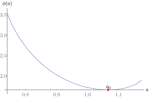
Figure 2: Plot of the function $\phi(a)$

Acknowledgements.

We would like to thanks Pietro Caputo and Matteo Quattropani for insightful discussions on the topic.

References

- Addario-Berry et al. [2020] L. Addario-Berry, B. Balle, and G. Perarnau. Diameter and Stationary Distribution of Random r-Out Digraphs. The Electronic Journal of Combinatorics, pages P3.28–P3.28, Aug. 2020. ISSN 1077-8926. doi: 10/ghd74q.
- Amini [2010] H. Amini. Bootstrap Percolation in Living Neural Networks. J Stat Phys, 141(3):459–475, Nov. 2010. ISSN 1572-9613. doi: 10/c53hx4.
- Athreya and Ney [1972] K. B. Athreya and P. E. Ney. Branching Processes. Grundlehren Der Mathematischen Wissenschaften. Springer-Verlag, Berlin Heidelberg, 1972. doi: 10/dft4.
- Blanchet and Stauffer [2013] J. Blanchet and A. Stauffer. Characterizing optimal sampling of binary contingency tables via the configuration model. Random Structures & Algorithms, 42(2):159–184, 2013. doi: 10/f4mtxh.
- Bordenave et al. [2018] C. Bordenave, P. Caputo, and J. Salez. Random walk on sparse random digraphs. Probab. Theory Relat. Fields, 170(3):933–960, Apr. 2018. ISSN 1432-2064. doi: 10/gc8nxk.
- Bordenave et al. [2019] C. Bordenave, P. Caputo, and J. Salez. Cutoff at the “entropic time” for sparse Markov chains. Probab. Theory Relat. Fields, 173(1):261–292, Feb. 2019. ISSN 1432-2064. doi: 10/ghcrhr.
- Cai and Devroye [2017] X. S. Cai and L. Devroye. The graph structure of a deterministic automaton chosen at random. Random Structures & Algorithms, 51(3):428–458, 2017. ISSN 1098-2418. doi: 10/gbtqgb.
- Cai and Perarnau [2020a] X. S. Cai and G. Perarnau. The giant component of the directed configuration model revisited. arXiv:2004.04998 [cs, math], Apr. 2020a. URL http://arxiv.org/abs/2004.04998.
- Cai and Perarnau [2020b] X. S. Cai and G. Perarnau. The diameter of the directed configuration model. arXiv:2003.04965 [cs, math], Mar. 2020b. URL http://arxiv.org/abs/2003.04965.
- Caputo and Quattropani [2020a] P. Caputo and M. Quattropani. Mixing time of PageRank surfers on sparse random digraphs. arXiv:1905.04993 [math], July 2020a. URL http://arxiv.org/abs/1905.04993.
- Caputo and Quattropani [2020b] P. Caputo and M. Quattropani. Stationary distribution and cover time of sparse directed configuration models. Probab. Theory Relat. Fields, Aug. 2020b. ISSN 1432-2064. doi: 10/ghd74v.
- Chatterjee [2007] S. Chatterjee. Stein’s method for concentration inequalities. Probab. Theory Relat. Fields, 138(1-2):305–321, Feb. 2007. ISSN 0178-8051, 1432-2064. doi: 10/fm2x4r.
- Chen et al. [2017] N. Chen, N. Litvak, and M. Olvera-Cravioto. Generalized PageRank on directed configuration networks. Random Structures & Algorithms, 51(2):237–274, 2017. ISSN 1098-2418. doi: 10/gbrth6.
- Cooper and Frieze [2004] C. Cooper and A. Frieze. The Size of the Largest Strongly Connected Component of a Random Digraph with a Given Degree Sequence. Combinatorics, Probability and Computing, 13(3):319–337, May 2004. doi: 10/cn8q5j.
- Cooper and Frieze [2012] C. Cooper and A. Frieze. Stationary distribution and cover time of random walks on random digraphs. J. Comb. Theory Ser. B, 102(2):329–362, Mar. 2012. ISSN 0095-8956. doi: 10/cv9wbh.
- Dembo and Zeitouni [2010] A. Dembo and O. Zeitouni. Large Deviations Techniques and Applications. Stochastic Modelling and Applied Probability. Springer-Verlag, Berlin Heidelberg, second edition, 2010. doi: 10.1007/978-3-642-03311-7.
- Graf [2016] A. Graf. On the Strongly Connected Components of Random Directed Graphs with given Degree Sequences. PhD thesis, University of Waterloo, 2016. URL http://hdl.handle.net/10012/10681.
- Janson [2009] S. Janson. The probability that a random multigraph is simple. Combinatorics, Probability and Computing, 18(1-2):205–225, 2009. doi: 10/bg4m2c.
- Li [2018] H. Li. Attack Vulnerability of Online Social Networks. In 2018 37th Chinese Control Conference (CCC), pages 1051–1056, July 2018. doi: 10/ggh2kg.
- Matthews [1988] P. Matthews. Covering Problems for Brownian Motion on Spheres. Ann. Probab., 16(1):189–199, Jan. 1988. ISSN 0091-1798, 2168-894X. doi: 10/c8q2r8.
- Molloy and Reed [2002] M. Molloy and B. Reed. Graph Colouring and the Probabilistic Method. Algorithms and Combinatorics. Springer-Verlag, Berlin Heidelberg, 2002. doi: 10.1007/978-3-642-04016-0.
- Petrov [1975] V. Petrov. Sums of Independent Random Variables. Ergebnisse Der Mathematik Und Ihrer Grenzgebiete. 2. Folge. Springer-Verlag, Berlin Heidelberg, 1975. doi: 10.1007/978-3-642-65809-9.
- Riordan and Wormald [2010] O. Riordan and N. Wormald. The diameter of sparse random graphs. Combin. Probab. Comput., 19(5-6):835–926, 2010. ISSN 0963-5483. doi: 10/dgp6hh.
- Sanders et al. [2020] D. P. Sanders, L. Benet, K. Agarwal, E. Gupta, B. Richard, M. Forets, yashrajgupta, E. Hanson, B. van Dyk, C. Rackauckas, S. Miclua-Câmpeanu, T. Koolen, C. Wormell, F. A. Vázquez, J. Grawitter, J. TagBot, K. O’Bryant, K. Carlsson, M. Piibeleht, Reno, R. Deits, S. Olver, T. Holy, kalmarek, and matsueushi. JuliaIntervals/IntervalArithmetic.jl: V0.17.5. Zenodo, June 2020. URL https://github.com/JuliaIntervals/IntervalArithmetic.jl.
- van der Hofstad [2016] R. van der Hofstad. Random Graphs and Complex Networks, volume 1 of Cambridge Series in Statistical and Probabilistic Mathematics. Cambridge University Press, Cambridge, England, 2016. doi: 10.1017/9781316779422.
- van der Hoorn and Olvera-Cravioto [2018] P. van der Hoorn and M. Olvera-Cravioto. Typical distances in the directed configuration model. Ann. Appl. Probab., 28(3):1739–1792, June 2018. ISSN 1050-5164, 2168-8737. doi: 10/ggh2ch.