Optimal Boundary Control of a Nonlinear Reaction Diffusion Equation via Completing
the Square and Al’brekht’s Method

Abstract

The two contributions of this paper are as follows. The first is the solution of an infinite dimensional, boundary controlled Linear Quadratic Regulator by the simple and constructive method of completing the square. The second contribution is the extension of Al’brekht’s method to the optimal stabilization of a boundary controlled, nonlinear Reaction Diffusion system.

I Introduction

In 1961 Al’brekht [1] showed how one could compute degree by degree the Taylor polynomials of the optimal cost and optimal feedback of a smooth, nonlinear, infinite horizon, finite dimensional optimal control problem provided the linear part of the dynamics and the quadratic part of the running cost satisfied the standard Linear Quadratic Regulator (LQR) conditions.

Recently [16] we showed how Al’brekht’s method could be generalized to infinite dimensional problems with distributed control. In this paper we show how Al’brekht’s method can be generalized to infinite dimensional problems with boundary control. In the next section we present and explicitly solve an LQR for the boundary control of a heated rod. We do this in a novel way, by completing the square in infinite dimensions. In Section Three we analyze the closed loop linear dynamics. In Section Four we show how Al’brekht’s method can be used to stabilize a nonlinear reaction diffusion equation using boundary control.

We are not the first to use Al’brekht’s method on infinite dimensional systems, see the works of Kunisch and coauthors [2], [3], [18]. Krstic, Vazquez and coauthors have had great success stabilizing infinite dimensional systems through boundary control where the nonlinearites are expressed by Volterra integral operators of increasing degrees using backstepping techniques, [17], [21]. In our extension of Al’brekht, we assume that the nonlinearites are given by Fredholm integral expressions of increasing degrees.

II Boundary Control of a Heated Rod

We consider a modification of Example 3.5.5 of Curtain and Zwart [8]. We have a rod of length one insulated at one end and heated/cooled at the other. The goal is to control the temperature to a constant set point which we conveniently take to be zero.

Let $0\leq x\leq 1$ be distance along the rod, $z(x,t)$ be the temperature of the rod at $x,t$ and $z^{0}(x)$ be the initial temperature distribution of the rod at $t=0$. The goal is to stabilize the temperature to $z=0$ as $t\to\infty$ using boundary control at $x=1$.

The rod is modeled by these equations

$$\frac{\partial z}{\partial t}(x,t) = \frac{\partial^{2}z}{\partial x^{2}}(x,t)$$ (1)

$$z(x,0) = z^{0}(x)$$ (2)

$$\frac{\partial z}{\partial x}(0,t) = 0$$ (3)

$$\frac{\partial z}{\partial x}(1,t) = \beta(u(t)-z(1,t))$$ (4)

for some positive constant $\beta$ where the control is $u(t)$, the temperature applied to the end of the rod.

First we study the open loop system where $u(t)=0$ for all $t\geq 0$. We consider the closed linear operator

$$Ah(x) = \frac{d^{2}h}{dx^{2}}(x)$$

where its domain is space of all $h\in{\bf L}_{2}[0,1]$ such that $h$ and $\frac{dh}{dx}$ are absolutely continuous and $\frac{dh}{dx}(0)=0$, $\frac{dh}{dx}(1)=-h(1)$. Because of the Neumann boundary condition at $x=0$, the eigenvectors are of form

$$\phi(x) = c\cos\nu x$$

for some constants $\nu$ and $c\neq 0$. The Robin boundary condition at $x=1$ implies that $\nu$ is a root of the equation

$$\nu\sin\nu = \beta\cos\nu$$ (5)

or equivalently

$$\nu = \beta\cot\nu$$ (6)

There is one root, $\nu_{n}$, of this equation in each open interval $(n\pi,(n+1/2)\pi)$ for $n=0,1,\ldots$. The $n^{th}$ root $\nu_{n}\to n\pi$ as $n\to\infty$. As $\beta\to 0$ the $n^{th}$ root $\nu_{n}\to n\pi$ and as $\beta\to\infty$ the $n^{th}$ root $\nu_{n}\to(n+1/2)\pi$. If $\beta=0$, $\nu_{n}=n\pi$ and we have an uncontrolled rod with no heat flux at either end. As $\beta\to\infty$ the $n^{th}$ root $\nu_{n}\to(n+1/2)\pi$. The corresponding eigenvalues are $\lambda_{n}=-\nu_{n}^{2}$.

If $\beta=1$, the first five roots are $\nu_{0}\approx 0.8603$, $\nu_{1}\approx 3.4256$, $\nu_{2}\approx 6.4373$, $\nu_{3}\approx 9.5293$ and $\nu_{4}\approx 12.6453$. So the five least stable eigenvalues are $\lambda_{0}=-\nu_{0}^{2}\approx-0.7402$, $\lambda_{1}=-\nu_{1}^{2}\approx-11.7349$, $\lambda_{2}=-\nu_{2}^{2}\approx-41.4388$, $\lambda_{3}=-\nu_{3}^{2}\approx-90.8082$ and $\lambda_{4}=-\nu_{4}^{2}\approx-159.9033$. Notice that as $n\to\infty$, $\nu_{n}$ is monotonically decreasing to $n\pi$ and $\lambda_{n}$ is monotonically increasing to $-n^{2}\pi^{2}$.

Because the Laplacian is self adjoint with respect to these boundary conditions, the eigenfunctions are orthogonal. We normalize them

$$\phi_{n}(x) = c_{n}\cos\nu_{n}x$$ (7)

where

$$c_{n} = \mbox{sign}(\cos\nu_{n})\ \sqrt{{4\nu_{n}\over 2\nu_{n}+\sin 2\nu_{n}}}$$ (8)

to get an orthonormal family satisfying $\phi_{n}(1)>0$. Because $\nu_{n}\in(n\pi,(n+1/2)\pi)$ it follows that $\mbox{sign}\ c_{n}=\mbox{sign}(\cos\nu_{n})=(-1)^{n}$ and $2\nu_{n}\in(2n\pi,(2n+1)\pi)$ so $\sin 2\nu_{n}$ is positive. This implies that $|c_{n}|\leq\sqrt{2}$ so

$$\phi_{n}(1) = c_{n}\cos\nu_{n}\ \leq\sqrt{2}\ |\cos\nu_{n}|\ \leq\ \sqrt{2}$$ (9)

Since $\nu_{n}-n\pi>0$ is monotonically decreasing to $0$ as $n\to\infty$, it follows that $c_{n}$ is monotonically decreasing to $\sqrt{2}$. Therefore maximum value of $c_{n}$ occurs at $c_{0}$.

The open loop system is asymptotically stable because all its eigenvalues are in the open left half plane. Let ${\bf Z}^{o}\subset{\bf L}_{2}[0,1]$ be the closure of the span of $\phi_{n}(x)$ for $i=0,1,2,\ldots$. The superscript ^o denotes that this is the closure of the domain of the open loop operator $A$. This operator is densely defined on ${\bf Z}^{o}$ and generates a strongly continuous semigroup. If $z^{0}(x)\in{\bf Z^{o}}$ then

$$z(x,t) = T^{o}(t)z^{0}(x)$$

$$= \sum_{i=0}^{\infty}e^{\lambda_{n}t}\phi_{n}(x)\ \int_{0}^{1}\phi_{n}(x_{1})z^{0}(x_{1})\ dx_{1}$$

Again the superscript on $T^{o}$ denotes that this is the open loop semigroup.

We seek a feedback control law of the form

$$u(t) = \int_{0}^{1}K(x)z(x,t)\ dx$$

to speed up the stabilization. To find $K(x)$ we solve a linear quadratic regulator (LQR). Minimize by choice of $u(t)$ the quantity

$$\int_{0}^{\infty}\iint_{\cal S}Q(x_{1},x_{2})z(x_{1},t)z(x_{2},t)\ dA\ dt$$ (10)

$$+\int_{0}^{\infty}Ru^{2}(t)$$

subject to (1, 2, 3, 4) where ${\cal S}$ is the unit square $[0,1]\times[0,1]$ and $dA=dx_{1}dx_{2}$.

We require that $R>0$ and $Q(x_{1},x_{2})$ is a symmetric function, $Q(x_{1},x_{2})=Q(x_{2},x_{1}),$ satisfying

$$0 \leq \iint_{\cal S}Q(x_{1},x_{2})\theta(x_{1})\theta(x_{2})\ dA$$

for any function $\theta(x)$. We allow $Q(x_{1},x_{2})$ to be a generalized function. For example if $Q(x_{1},x_{2})=Q(x_{1})\delta(x_{1}-x_{2})$, where $Q(x_{1})\geq 0$ for each $x_{1}$ and $\delta(x_{1}-x_{2})$ is the Dirac $\delta$ function then

$$\iint_{\cal S}Q(x_{1},x_{2})z(x_{1},t)z(x_{2},t)\ dA=\int_{0}^{1}Q(x)z^{2}(x,t)\ dx$$

Let $P(x_{1},x_{2})$ be any continuous, symmetric function of $(x_{1},x_{2})$. Assume that the control trajectory $u(t)$ results in $z(x,t)\to 0$ as $t\to\infty$. We know that such control trajectories exist because the open loop rod, $u(t)=0$, is asymptotically stable. By the Fundamental Theorem of Calculus

$$0 = \iint_{\cal S}P(x_{1},x_{2})z^{0}(x_{1})z^{0}(x_{2})\ dA$$

$$+ \int_{0}^{\infty}\iint_{\cal S}{d\over dt}\left(P(x_{1},x_{2})z(x_{1},t)z(x_{2},t)\right)\ dA\ dt$$

so

$$0=\iint_{\cal S}P(x_{1},x_{2})z^{0}(x_{1})z^{0}(x_{2})\ dA$$ (11)

$$+\int_{0}^{\infty}\iint_{\cal S}P(x_{1},x_{2})\frac{\partial^{2}z}{\partial x_{1}^{2}}(x_{1},t)z(x_{2},t)$$

$$+P(x_{1},x_{2})z(x_{1},t)\frac{\partial^{2}z}{\partial x_{2}^{2}}(x_{2},t)\ dA\ dt$$

We assume that $P(x_{1},x_{2})$ satisfies Neumann boundary conditions at $x_{i}=0$

$$\frac{\partial P}{\partial x_{1}}(0,x_{2}) = 0$$ (12)

$$\frac{\partial P}{\partial x_{2}}(x_{1},0) = 0$$ (13)

and Robin boundary conditions at $x_{i}=1$

$$\frac{\partial P}{\partial x_{1}}(1,x_{2}) = -\beta P(1,x_{2})$$ (14)

$$\frac{\partial P}{\partial x_{2}}(x_{1},1) = -\beta P(x_{1},1)$$ (15)

Because of the symmetry of $P(x_{1},x_{2})$, (12) is equivalent to (13) and (14) is equivalent to (15).

When we integrate (11) by parts twice we get the equation

$$0 = \iint_{\cal S}P(x_{1},x_{2})z^{0}(x_{1})z^{0}(x_{2})\ dA$$

$$+ \int_{0}^{\infty}\iint_{\cal S}\nabla^{2}P(x_{1},x_{2})z(x_{1},t)z(x_{2},t)\ dA\ dt$$

$$+ \int_{0}^{\infty}\int_{0}^{1}P(1,x_{2})\beta u(t)z(x_{2},t)\ dx_{2}\ dt$$

$$+ \int_{0}^{\infty}\int_{0}^{1}P(x_{1},1)z(x_{1},t)\beta u(t)\ dx_{1}\ dt\$$

where $\nabla^{2}$ is the two dimensional Laplacian.

We add the right side of (II) to the criterion (10) to be minimized to get the equivalent criterion

$$\iint_{\cal S}P(x_{1},x_{2})z^{0}(x_{1})z^{0}(x_{2})\ dA$$

$$+ \int_{0}^{\infty}\iint_{\cal S}\left(\nabla^{2}P(x_{1},x_{2})+Q(x_{1},x_{2})\right)$$

$$\times z(x_{1},t)z(x_{2},t)\ dA\ dt$$

$$+ \int_{0}^{\infty}\int_{0}^{1}P(1,x_{2})\beta u(t)z(x_{2},t)\ dx_{2}\ dt$$

$$+ \int_{0}^{\infty}\int_{0}^{1}P(x_{1},1)z(x_{1},t)\beta u(t)\ dx_{1}\ dt$$

$$+ \int_{0}^{\infty}Ru^{2}(t)\ dt$$

Suppose this criterion can be written as a double integral with respect to the initial state and a time integral of a perfect square involving the control. If the latter can be made zero by the proper choice of the control then the optimal cost is the double integral with respect to the initial state.

So we would like to chose $K(x)$ so that the time integrand in (II) is a perfect square. In other words we want (II) to be of the form

$$0=\iint_{\cal S}P(x_{1},x_{2})z^{0}(x_{1})z^{0}(x_{2})\ dA$$ (18)

$$+\int_{0}^{\infty}\iint_{\cal S}R\left(u(t)-K(x_{1})z(x_{1},t)\right)$$

$$\times\left(u(t)-K(x_{2})z(x_{2},t)\right)\ dA\ dt$$

Clearly the terms quadratic in $u(t)$ match so we equate the terms involving $u(t)$ and $z(x_{1},t)$,

$$\int_{0}^{\infty}\int_{0}^{1}P(x_{1},1)z(x_{1},t)\beta u(t)\ dx_{1}dt$$

$$=-\int_{0}^{\infty}\int_{0}^{1}K(x_{1})Rz(x_{1},t)u(t)\ dx_{1}dt$$

To make these equal we set

$$K(x_{1})=-\beta R^{-1}P(x_{1},1)$$ (19)

By the symmetry of $P(x_{1},x_{2})$, $K(x_{2})=-\beta R^{-1}P(1,x_{2})$.

Finally we equate the terms involving $z(x_{1},t)$ and $z(x_{2},t)$,

$$\iint_{\cal S}\left(\nabla^{2}P(x_{1},x_{2})+Q(x_{1},x_{2})\right)$$

$$\times z(x_{1},t)z(x_{2},t)\ dA\ dt$$

$$=R\int_{0}^{\infty}\iint_{\cal S}K(x_{1})K(x_{2})z(x_{1},t)z(x_{2},t)\ dA\ dt$$

This yields what we call a Riccati PDE

$$\nabla^{2}P(x_{1},x_{2})+Q(x_{1},x_{2})=RK(x_{1})K(x_{2})$$

$$=\beta^{2}R^{-1}P(x_{1},1)P(1,x_{2})$$ (20)

Since we only assumed that $P(x_{1},x_{2})$ is continuous and $Q(x_{1},x_{2})$ might equal $Q(x_{1})\delta(x_{1}-x_{2})$, this is to be interpreted in the weak sense, if $\theta(x)$ is $C^{2}$ on $0\leq x\leq 1$ then

$$\iint_{\cal S}\left(\nabla^{2}P(x_{1},x_{2})+Q(x_{1},x_{2})\right)\theta(x_{1})\theta(x_{2})\ dA$$

$$=\iint_{\cal S}\beta^{2}R^{-1}P(x_{1},1)P(1,x_{2})\theta(x_{1})\theta(x_{2})\ dA$$

where the evaluations are done using integration by parts.

The boundary conditions (12, 13 14, 15) are also to be interpreted in the weak sense

$$0 = \int_{0}^{1}\frac{\partial P}{\partial x_{1}}(0,x_{2})\theta(x_{2})\ dx_{2}$$

$$0 = \int_{0}^{1}\frac{\partial P}{\partial x_{2}}(x_{1},0)\theta(x_{1})\ dx_{1}$$

$$0 = \int_{0}^{1}\left(\frac{\partial P}{\partial x_{1}}(1,x_{2})+\beta R^{-1}P(1,x_{2})\right)\theta(x_{2})\ dx_{2}$$

$$0 = \int_{0}^{1}\left(\frac{\partial P}{\partial x_{2}}(x_{1},1)+\beta R^{-1}P(x_{1},1)\right)\theta(x_{1})\ dx_{1}$$

If we can solve the Riccati PDE subject to these boundary conditions then clearly the optimal cost starting from $z^{0}(x)$ is a quadratic functional of the initial state

$$\iint_{\cal S}P(x_{1},x_{2})z^{0}(x_{1})z^{0}(x_{2})\ dA$$

and the optimal feedback is a linear functional of the current state

$$u(t) = \int_{0}^{1}K(x)z(x,t)\ dx$$ (21)

$$= -\beta R^{-1}\int_{0}^{1}P(x,1)z(x,t)\ dx$$

We assume that the solution to the Riccati PDE has an expansion in the open loop eigenfunctions (7),

$$P(x_{1},x_{2}) = \sum_{n_{1},n_{2}=0}^{\infty}P_{n_{1},n_{2}}\phi_{n_{1}}(x_{1})\phi_{n_{2}}(x_{2})$$ (22)

In abuse of notation we use the symbol $P$ to denote both a function $P(x_{1},x_{2})$ and a coefficient $P_{n_{1},n_{2}}$. The proper meaning should be clear from context. Clearly any such expansion satisfies the boundary conditions (12, 13, 14, 15). Then

$$K(x) = -\beta R^{-1}\sum_{n_{1},n_{2}=0}^{\infty}P_{n_{1},n_{2}}\phi_{n_{1}}(1)\phi_{n_{2}}(x)$$ (23)

Because we seek a symmetric weak solution without loss of generality $P_{n_{1},n_{2}}=P_{n_{2},n_{1}}$.

We also assume that $Q(x_{1},x_{2})$ has a similar expansion,

$$Q(x_{1},x_{2}) = \sum_{i_{1},i_{2}=0}^{\infty}Q_{n_{1},n_{2}}\phi_{n_{1}}(x)\phi_{n_{2}}(x)$$ (24)

We plug these into (II) and get an algebraic Riccati equation for the infinite dimensional matrix $P_{n_{1},n_{2}}$,

$$(\lambda_{n_{1}}+\lambda_{n_{2}})P_{n_{1},n_{2}}+Q_{n_{1},n_{2}}$$ (25)

$$=\beta^{2}R^{-1}\sum_{m_{1},m_{2}=0}^{\infty}P_{n_{1},m_{1}}P_{n_{2},m_{2}}\phi_{m_{1}}(1)\phi_{m_{2}}(1)$$

To simplify the notation henceforth we assume

$$\beta = 1$$ (26)

$$Q(x_{1},x_{2}) = \delta(x_{1}-x_{2})$$

$$R = 1$$

where $\delta(x_{1}-x_{2})$ is the Dirac $\delta$. Then by Parseval’s equality

$$Q_{n_{1},n_{2}} = \delta_{n_{1},n_{2}}$$

where $\delta_{n_{1},n_{2}}$ is the Kronecker $\delta$.

Let $\Pi$ denote the infinite dimensional matrix $[P_{n_{1},n_{2}}]$. Then (25) is the algebraic Riccati equation

$$F^{\prime}\Pi+\Pi F+Q = \Pi GR^{-1}G^{\prime}\Pi$$

of the infinite dimensional linear quadratic system where

$$F = \left[\begin{array}[]{ccccccccc}\lambda_{1}&0&0&\ldots\\ 0&\lambda_{2}&0&\ldots\\ 0&0&\ddots&\end{array}\right]$$

$$G = \left[\begin{array}[]{ccccccccc}\phi_{1}(1)\\ \phi_{2}(1)\\ \vdots\end{array}\right]$$

$$Q = \left[\begin{array}[]{ccccccccc}1&0&0&\ldots\\ 0&1&0&\ldots\\ &&\ddots&\end{array}\right]$$

$$R = 1$$

We denote our first guess at a solution to (25) by $P^{(1)}_{n_{1},n_{2}}$ and we take it to be diagonal,

$$P^{(1)}_{n_{1},n_{2}}=\delta_{n_{1},n_{2}}P^{(1)}_{n_{1},n_{2}}$$ (30)

Then we get a sequence of quadratic equations for $P^{(1)}_{n,n}$,

$$0 = \phi^{2}_{n}(1)\left(P^{(1)}_{n,n}\right)^{2}-2\lambda_{n,n}P^{(1)}_{n,n}-1$$ (31)

Clearly we wish to take the positive root so we assume

$$P^{(1)}_{n,n}={\lambda_{n}+\sqrt{\lambda_{n}^{2}+\phi_{n}^{2}(1)}\over\phi_{n}^{2}(1)}$$ (32)

But we need to check if the off-diagonal terms satisfy (25). If (30) holds then when $n_{1}\neq n_{2}$ (25) becomes

$$0 = \sum_{m_{1},m_{2}=0}^{\infty}P^{(1)}_{n_{1},m_{1}}P^{(1)}_{n_{2},m_{2}}\phi_{m_{1}}(1)\phi_{m_{2}}(1)$$

$$= P^{(1)}_{n_{1},n_{1}}P^{(1)}_{n_{2},n_{2}}\phi_{n_{1}}(1)\phi_{n_{2}}(1)\ \neq\ 0$$

So we conclude that the solution to (25) is not diagonal.

Given $P^{(k)}_{n_{1},n_{2}}$ we define $P^{(k+1)}_{n_{1},n_{2}}$ by the equation

$$(\lambda_{n_{1}}+\lambda_{n_{2}})P^{(k+1)}_{n_{1},n_{2}}+Q_{n_{1},n_{2}}$$ (33)

$$=\sum_{m_{1},m_{2}=0}^{\infty}P^{(k)}_{n_{1},m_{1}}P^{(k)}_{n_{2},m_{2}}\phi_{m_{1}}(1)\phi_{m_{2}}(1)$$

Then we define

$$P^{(k+1)}(x_{1},x_{2}) = \sum_{n_{1},n_{2}=0}^{\infty}P^{(k+1)}_{n_{1},n_{2}}\phi_{n_{1}}(x_{1})\phi_{n_{2}}(x_{2})$$

$$K^{(k+1)}(x) = \sum_{n_{1},n_{2}=0}^{\infty}P^{(k+1)}_{n_{1},n_{2}}\phi_{n_{1}}(1)\phi_{n_{2}}(x)$$

Although it may not be obvious this is variation of the familiar policy iteration scheme for solving an optimal control problem. Our $k^{th}$ approximation of the optimal cost of starting at $z^{0}(x)$ is

$$\iint_{\cal S}P^{(k)}(x_{1},x_{2})z^{0}(x_{1})z^{0}(x_{2})\ dA$$

where

$$P^{(k)}(x_{1},x_{2}) = \sum_{n_{1},n_{2}=0}^{\infty}P^{(k)}_{n_{1},n_{2}}\phi_{n_{1}}(x_{1})\phi_{n_{2}}(x_{2})$$

Given this approximation then we plug $P^{(k)}(x_{1},x_{2})$ into (II) to get

$$\iint_{\cal S}P^{(k)}(x_{1},x_{2})z^{0}(x_{1})z^{0}(x_{2})\ dA$$

$$+ \int_{0}^{\infty}\iint_{\cal S}\left(\nabla^{2}P^{(k)}(x_{1},x_{2})+\delta(x_{1}-x_{2})\right)$$

$$\times z(x_{1},t)z(x_{2},t)\ dA\ dt$$

$$+ \int_{0}^{\infty}\int_{0}^{1}P^{(k)}(1,x_{2})u(t)z(x_{2},t)\ dx_{2}\ dt$$

$$+ \int_{0}^{\infty}\int_{0}^{1}P^{(k)}(x_{1},1)z(x_{1},t)u(t)\ dx_{1}\ dt$$

$$+ \int_{0}^{\infty}u^{2}(t)\ dt$$

To find the $k^{th}$ approximation of the optimal control we minimize this expression with respect to $u$ and obtain

$$u^{(k)}(t) = -\int_{0}^{1}P^{(k)}(x_{1},1)z(x_{1},t)\ dx_{1}$$

so the $k^{th}$ approximation of the optimal gain is

$$K^{(k)}(x_{1}) = -P^{(k)}(x_{1},1)$$

Let $z^{k}(x,t)$ be the solution of (1, 2, 3, 4) when $u(t)=u^{(k)}(t)$. The $(k+1)^{th}$ approximation of the optimal cost is

$$\iint_{\cal S}P^{(k)}(x_{1},x_{2})z^{0}(x_{1})z^{0}(x_{2})\ dA$$

$$=\int_{0}^{\infty}\int_{0}^{1}\left(z^{k}(x,t)\right)^{2}+\left(u^{(k)}(t)\right)^{2}\ dx\ dt$$

Then for any $z^{0}(x)$ the sequence of scalars

$$\iint_{\cal S}P^{(k)}(x_{1},x_{2})z^{0}(x_{1})z^{0}(x_{2})\ dA$$

is nonincreasing in $k$ and bounded below by zero hence it is convergent. It follows that the Fourier coefficients $P^{(k)}_{n_{1},n_{2}}$ are also convergent.

We compute an approximation to the upper left block of $P^{(50)}_{n_{1},n_{2}}$ by truncating the iteration (33) to

$$(\lambda_{n_{1}}+\lambda_{n_{2}})P^{(k+1)}_{n_{1},n_{2}}+Q_{n_{1},n_{2}}$$

$$=\sum_{m_{1},m_{2}=0}^{10}P^{(k)}_{n_{1},m_{1}}P^{(k)}_{n_{2},m_{2}}\phi_{m_{1}}(1)\phi_{m_{2}}(1)$$

Then after $50$ iterations the upper left block of $P^{(50)}_{n_{1},n_{2}}$ is approximately

$$\left[\begin{array}[]{ccccccccc}0.5757&-0.0018&-0.0002&-0.0000\\ -0.0018&0.0425&-0.0000&-0.0000\\ -0.0002&-0.0000&0.0121&-0.0000\\ -0.0000&-0.0000&-0.0000&0.0055\end{array}\right]$$

Notice how strongly diagonally dominant this is and how the diagonal elements are decreasing quite fast.

III Closed Loop Eigenvalues and Eigenvectors

We continue to assume that (26) holds. The boundary feedback does not appear in the closed loop dynamics, it is still

$$\frac{\partial z}{\partial t}(x,t) = \frac{\partial^{2}z}{\partial x^{2}}(x,t)$$

but the boundary conditions are changed by the feedback. The boundary condition at $x=0$ is still the Neumann boundary condition (3) but the Robin boundary condition (4) at $x=1$ is replaced by

$$\frac{\partial z}{\partial x}(1,t)=\int_{0}^{1}K(x_{1})z(x_{1},t)\ dx_{1}-z(1,t)$$ (36)

$$=\sum_{n_{1},n_{2}=0}^{\infty}P_{n_{1},n_{2}}\phi_{n_{2}}(1)\int_{0}^{1}\phi_{n_{1}}(x)z(x,t)\ dx-z(1,t)$$

Note that this nonstandard boundary condition (36) is linear in $z(x,t)$.

Because of the Neumann BC at $x=0$ we know that the unit normal closed loop eigenvectors are of the form

$$\psi(x) = c(\rho)\cos\rho x$$ (37)

for some $\rho>0$ where the normalizing constant is given by

$$c(\rho) = \mbox{sign}(\cos\rho)\sqrt{{4\rho\over 2\rho+\sin 2\rho}}$$ (38)

The $\rho$ are chosen so that $g(\rho)=0$ where

$$g(\rho)=\rho\sin\rho-\cos\rho$$ (39)

$$-\sum_{n_{1},n_{2}=0}^{\infty}P_{n_{1},n_{2}}\phi_{n_{2}}(1)\int_{0}^{1}\phi_{n_{1}}(x_{1})\cos\rho x_{1}\ dx_{1}$$

The one dimensional Laplacian is not self adjoint under these boundary conditions (3, 36) so there is no reason to expect that the closed loop eigenfunctions are orthogonal.

If $n>10$ then $P_{n,n}\leq{1\over 2|\lambda_{10}|}\leq{1\over 200\pi^{2}}\approx 0.0005$, so to approximate the first few $\rho_{n}$ we truncate (39) to

$$\rho\sin\rho-\cos\rho$$ (40)

$$=\sum_{n_{1}.n_{2}=0}^{10}P_{n_{1},n_{2}}\phi_{n_{2}}(1)\int_{0}^{1}\phi_{n_{1}}(x_{1})\psi(x_{1})\ dx_{1}$$

We solve (40) by Newton’s method starting at $\rho=1.05\nu_{n}$ for $n=0,1,2,3,4$. The result is $\rho_{0}\approx 0.9982$, $\rho_{1}\approx 3.4381$, $\rho_{2}\approx 6.4391$, $\rho_{3}\approx 9.5299$ and $\rho_{4}\approx 12.6455$.

The first five closed loop eigenvalues are approximately $\mu_{0}\approx-\rho_{0}^{2}=-0.9964$, $\mu_{1}\approx-\rho_{1}^{2}=-11.8202$, $\mu_{2}\approx-\rho_{2}^{2}=-41.4618$, $\mu_{3}\approx-\rho_{3}^{2}=-90.8190$ and $\mu_{4}\approx-\rho_{4}^{2}=-159.9095$. Recall the first five open loop eigenvalues are approximately $\lambda_{0}\approx-0.7401$, $\lambda_{1}\approx-11.7347$, $\lambda_{2}\approx-41.4620$, $\lambda_{3}\approx-90.8192$ and $\lambda_{4}\approx-159.9095$. Notice how close $\mu_{n}$ and $\lambda_{n}$ are if $n>0$. The boundary feedback has a significant effect on the least stable open loop eigenvalue but less so on the rest of the open loop eigenvalues because they are already so stable it would cost to much control energy to significantly increase their stability.

IV Boundary Control of a Nonlinear Reaction Diffusion Equation

To the above system we add a destabilizing nonlinear term to obtain the boundary controlled reaction diffusion system

$$\frac{\partial z}{\partial t}(x,t) = \frac{\partial^{2}z}{\partial x^{2}}(x,t)+\alpha z^{2}(x,t)$$ (41)

$$z(x,0) = z^{0}(x)$$ (42)

$$\frac{\partial z}{\partial x}(0,t) = 0$$ (43)

$$\frac{\partial z}{\partial x}(1,t) = (u(t)-z(1,t))$$ (44)

for some positive constant $\alpha$. Vazquez and Krstic [21] used backstepping to stabilize a similar system with $\alpha=1$. They assumed a different boundary condition at $x=1$, namely direct control of the heat flux,

$$\frac{\partial z}{\partial x}(1,t) = u(t)$$

To find a feedback to stabilize this system we consider the nonlinear quadratic optimal control of minimizing (10) subject to (41, 42, 43, 44).

It is well known [11] that this system cannot be globally stabilized but we are only interested in local stabilization around $z=0$. The reason is that this is a mathematical model of a physical system and the model is not globally valid, there is an absolute zero temperature that the rod cannot go below and at a sufficiently high temperature the rod will melt. So global stabilization is of mathematical but not of physical interest.

Let $P(x_{1},x_{2})$ be the solution of the Riccati PDE (II) and $K(x)$ be the gain of the optimal linear feedback (19). In abuse of notation let $P(x_{1},x_{2},x_{3})$ be a symmetric function of three variables. We distinguish between $P(x_{1},x_{2})$ and $P(x_{1},x_{2},x_{3})$ by the number of arguments. Symmetric means that the value of the function is invariant under any permutation of the three variables.

We further assume that $P(x_{1},x_{2},x_{3})$ weakly satisfies Neumann boundary conditions at $x_{1}=0$

$$\frac{\partial P}{\partial x_{1}}(0,x_{2},x_{3}) = 0$$ (45)

and Robin boundary conditions at $x_{1}=1$

$$\frac{\partial P}{\partial x_{1}}(1,x_{2},x_{3}) = -P(1,x_{2},x_{3})$$ (46)

By symmetry, similar boundary conditions hold at $x_{2}=0,1$ and $x_{3}=0,1$.

Assume also that the optimal feedback takes the form

$$u(t) = \int_{0}^{1}K(x_{1})z(x_{1},t)\ dx_{1}$$

$$+\iint_{\cal S}K(x_{1},x_{2})z(x_{1},t)z(x_{2},t)\ dA$$

$$+O(\left\|z(x,t)\right\|)^{3}$$

where

$$\left\|z(x,t)\right\|^{2} = \int_{0}^{1}|z(x,t)|^{2}\ dx$$

Again we distinguish between the optimal linear feedback gain $K(x_{1})$ and the optimal quadratic feedback gain $K(x_{1},x_{2})$ by the number of arguments

Again by the Fundamental Theorem of Calculus if the control trajectory $u(t)$ takes $z(x,t)\to 0$ as $t\to\infty$ then

$$0=\iint_{\cal S}P(x_{1},x_{2})z^{0}(x_{1})z^{0}(x_{2})\ dA$$ (49)

$$+\iiint_{\cal C}P(x_{1},x_{2},x_{3})z^{0}(x_{1})z^{0}(x_{2})z^{0}(x_{3})\ dV$$

$$+\int_{0}^{\infty}\iint_{\cal S}{d\over dt}\left(P(x_{1},x_{2})z(x_{1},t)z(x_{2},t)\right)\ dA\ dt$$

$$+\int_{0}^{\infty}\iiint_{\cal C}{d\over dt}\left(P(x_{1},x_{2},x_{3})z(x_{1},t)z(x_{2},t)z(x_{3},t)\right)$$

$$\times dV\ dt+O(\left\|z(x,t)\right\|)^{4}$$

where ${\cal C}$ denotes the unit cube $[0,1]\times[0,1]\times[0,1]$ and $dV$ is the volume element $dV=dx_{1}dx_{2}dx_{3}$.

Because $P(x_{1},x_{2})$ is the solution of the Riccati PDE, the terms quadatic in $z$ in the time integral drop out. But we pick up cubic terms from the boundary when we integrate (49) by parts twice. We use the symmetry of $P(x_{1},x_{2})$ and $P(x_{1},x_{2},x_{3})$ to condense them. Then we obtain

$$0=\iint_{\cal S}P(x_{1},x_{2})z^{0}(x_{1})z^{0}(x_{2})\ dA$$ (50)

$$+\int_{0}^{\infty}\iiint_{\cal C}P(x_{1},x_{2},x_{3})z^{0}(x_{1})z^{0}(x_{2})z^{0}(x_{3})\ dV$$

$$+2\alpha\int_{0}^{\infty}\iint_{\cal S}P(x_{1},x_{2})z^{2}(x_{1},t)z(x_{2},t)\ dA\ dt$$

$$+3\int_{0}^{\infty}\iiint_{\cal C}P(x_{1},x_{2},x_{3})\frac{\partial^{2}z}{\partial x_{1}^{2}}(x_{1},t)$$

$$\times z(x_{2},t)z(x_{3},t)dV\ dt$$

$$+3\int_{0}^{\infty}\iiint_{\cal C}P(1,x_{2},x_{3})K(x_{1})$$

$$\times z(x_{1},t)z(x_{2},t)z(x_{3},t)\ dV\ dt$$

$$+2\int_{0}^{\infty}\iiint_{\cal C}P(x_{1},1)K(x_{2},x_{3})$$

$$\times z(x_{1},t)z(x_{2},t)z(x_{3},t)\ dV\ dt+O(\left|z(x,t)\right|)^{4}$$

If we integrate (50) by parts twice we get the equation

$$0=\iint_{\cal S}P(x_{1},x_{2})z^{0}(x_{1})z^{0}(x_{2})\ dA$$ (51)

$$+\iiint_{\cal C}P(x_{1},x_{2},x_{3})z^{0}(x_{1})z^{0}(x_{2})z^{0}(x_{3})\ dV$$

$$+\int_{0}^{\infty}\iiint_{\cal C}\nabla^{2}P(x_{1},x_{2},x_{3})$$

$$\times z(x_{1},t)z(x_{2},t)z(x_{3},t)\ dVdt$$

$$+2\alpha\int_{0}^{\infty}\iint_{\cal S}P(x_{1},x_{2})z^{2}(x_{1},t)z(x_{2},t)\ dA\ dt$$

$$+3\int_{0}^{\infty}\iiint_{\cal C}P(1,x_{2},x_{3})K(x_{1})$$

$$\times z(x_{1},t)z(x_{2},t)z(x_{3},t)\ dVdt$$

$$+2\int_{0}^{\infty}\iiint_{\cal C}P(x_{1},1)K(x_{2},x_{3})$$

$$\times z(x_{1},t)z(x_{2},t)z(x_{3},t)\ dVdt+O(\left\|z(x,t)\right\|)^{4}$$

where $\nabla^{2}$ is now the three dimensional Laplacian. This equation (51) is not symmetric in $x_{1},x_{2},x_{3}$ but we are looking for a symmetric weak solution. If $P(x_{1},x_{2},x_{3})$ is a weak solution that is not symmetric then we can get a symmetric weak solution by averaging over all permutations of $x_{1},x_{2},x_{3}$.

We have cancelled the quadratic terms in the criterion by our choice $P(x_{1},x_{2})$ and $K(x)$ but the quadratic term in the feedback generates a cubic term in the criterion of the form

$$2\int_{0}^{\infty}\int_{0}^{1}\int_{0}^{1}\int_{0}^{1}K(x_{1})K(x_{2},x_{3})$$

$$\times z(x_{1},t)z(x_{2},t)z(x_{3},t)\ dV\ dt$$

Because of (19) this equals

$$-2\int_{0}^{\infty}\iiint_{\cal C}P(x_{1},1)K(x_{2},x_{3})$$

$$\times z(x_{1},t)z(x_{2},t)z(x_{3},t)\ dV\ dt$$

and so this cancels out the last term in (51).

So the new criterion to be minimized is

$$0=\iint_{\cal S}P(x_{1},x_{2})z^{0}(x_{1})z^{0}(x_{2})\ dA$$ (52)

$$+\iiint_{\cal C}P(x_{1},x_{2},x_{3})z^{0}(x_{1})z^{0}(x_{2})z^{0}(x_{3})\ dV$$

$$+\int_{0}^{\infty}\iiint_{\cal C}\nabla^{2}P(x_{1},x_{2},x_{3})$$

$$\times z^{0}(x_{1})z^{0}(x_{2})z^{0}(x_{3})\ dV\ dt$$

$$+3\int_{0}^{\infty}\iiint_{\cal C}P(x_{1},x_{2},1)K(x_{3})$$

$$\times z(x_{1})z(x_{2})z(x_{3})\ dV\ dt$$

$$+2\alpha\int_{0}^{\infty}\iint_{\cal S}P(x_{1},x_{2})z^{2}(x_{1},t)z(x_{2},t)\ dA\ dt$$

Notice the quadratic optimal gain $K(x_{1},x_{2})$ does not appear in this equation so we can solve for cubic kernel $P(x_{1},x_{2},x_{3})$ of the optimal cost independently of $K(x_{1},x_{2})$.

We assume that $P(x_{1},x_{2},x_{3})$ is a symmetric weak solution to the symmetric linear elliptic PDE

$$0=\nabla^{2}P(x_{1},x_{2},x_{3})$$

$$+P(1,x_{2},x_{3})K(x_{1})$$

$$+P(x_{1},1,x_{3})K(x_{2})$$

$$+P(x_{1},x_{2},1)K(x_{3})$$

$$+{2\alpha\over 3}\left(P(x_{1},x_{2})\delta(x_{1}-x_{3})+P(x_{2},x_{3})\delta(x_{2}-x_{1})\right.$$

$$\left.+P(x_{3},x_{1})\delta(x_{3}-x_{2})\right)$$

subject to the weak boundary conditions (45, 46). Then the optimal cost is

$$\iint_{\cal S}P(x_{1},x_{2})z^{0}(x_{1})z^{0}(x_{2})\ dA$$ (54)

$$+\iiint_{\cal C}P(x_{1},x_{2},x_{3})z^{0}(x_{1})z^{0}(x_{2})z^{0}(x_{3})\ dV$$

$$+O(\left\|z^{0}(x)\right\|^{4})$$

where

$$\left\|z^{0}(x)\right\|^{2}=\int_{0}^{1}\left(z^{0}(x)\right)^{2}\ dx$$

To find the quadratic optimal feedback gain we start by noting that the optimal cost starting from $z^{0}(x)$ is (54).

Let $u^{*}(t)$ be the optimal control trajectory starting from $z^{0}(x)$ then by arguments similar to the above we obtain

$$\int_{0}^{\infty}\int_{0}^{1}z^{2}(x,t)\ dx+(u^{*}(t))^{2}\ dx\ dt$$

$$+\int_{0}^{\infty}\int_{[0,1]^{2}}\left(\nabla^{2}P(x_{1},x_{2})+2\alpha_{1}\right)$$

$$\times z(x_{1},t)z(x_{2},t)\ dA\ dt$$

$$+\int_{0}^{\infty}\int_{[0,1]^{3}}\nabla^{2}P(x_{1},x_{2},x_{3})$$

$$\times z(x_{1},t)z(x_{2},t)z(x_{3},t)\ dV\ dt$$

$$+2\alpha_{2}\int_{0}^{\infty}\int_{[0,1]^{2}}\nabla^{2}P(x_{1},x_{2})z^{2}(x_{1},t)z(x_{2},t)$$

$$+2\int_{0}^{\infty}\int_{0}^{1}P(x_{1},1)z(x_{1},t)u^{*}(t)\ dx_{1}\ dt$$

$$+3\int_{0}^{\infty}\int_{[0,1]^{2}}P(x_{1},x_{2},1)$$

$$\times z(x_{1},t)z(x_{2},t)u^{*}(t)\ dA\ dt$$

$$+O(\left\|z^{0}(x)\right\|^{4})$$

We replace $u^{*}(t)$ by $u^{*}(t)+\epsilon\delta u(t)$ in this expression and differentiate with respect to $\epsilon$ at $\epsilon=0$ to obtain the expression

$$2\int_{0}^{\infty}u^{*}(t)\delta u(t)\ dt$$

$$+2\int_{0}^{\infty}\int_{0}^{1}P(x_{1},1)z(x_{1},t)\delta u(t)\ dx_{1}\ dt$$

$$+3\int_{0}^{\infty}\int_{[0,1]^{2}}P(x_{1},x_{2},1)z(x_{1},t)z(x_{2},t)\delta u(t)\ dA\ dt$$

$$+O(\left\|z^{0}(x)\right\|^{4})$$

Since $u^{*}(t)$ is the optimal control trajectory this quantity must be zero for any $\delta u(t)$ so the coefficient of $\delta u(t)$ must vanish for each $t$. This leads to the expressions for the linear and quadratic parts of the optimal feedback,

$$u^{*}(t) = \int_{0}^{1}K(x_{1})z(x_{1},t)\ dx_{1}$$

$$+\int_{[0,1]^{2}}K(x_{1},x_{2})z(x_{1},t)z(x_{2},t)\ dA$$

$$+O(\left\|z^{0}(x)\right\|^{3})$$

where

$$K(x_{1}) = -P(x_{1},1)$$ (55)

$$K(x_{1},x_{2}) = -{3\over 2}P(x_{1},x_{2},1)$$ (56)

Again we expand $P(x_{1},x_{2},x_{3})$ in terms of the orthonormal eigenfunctions of the unforced system

$$P(x_{1},x_{2},x_{3})=\sum_{n_{1},n_{2},n_{3}=1}^{\infty}P_{n_{1},n_{2},n_{3}}\phi_{n_{1}}(x_{1})\phi_{n_{2}}(x_{2})\phi_{n_{3}}(x_{3})$$

where $P_{n_{1},n_{2},n_{3}}$ is a three tensor that is symmetric in its three indices. The symmetric linear elliptic PDE (IV) is then equivalent to

$$0=\left(\lambda_{n_{1}}+\lambda_{n_{2}}+\lambda_{n_{3}}\right)P_{n_{1},n_{2},n_{3}}$$ (57)

$$-\sum_{m_{1},m_{2}=1}^{\infty}P_{m_{1},n_{2},n_{3}}P_{m_{1},m_{2}}\phi_{m_{2}}(1)$$

$$-\sum_{m_{1},m_{2}=1}^{\infty}P_{n_{1},m_{1},n_{3}}P_{m_{1},m_{2}}\phi_{m_{2}}(1)$$

$$-\sum_{m_{1},m_{2}=1}^{\infty}P_{n_{1},n_{2},m_{1}}P_{m_{1},m_{2}}\phi_{m_{2}}(1)$$

$$+{2\alpha\over 3}\left(P_{n_{1},n_{2}}\delta_{n_{1},n_{3}}+P_{n_{2},n_{3}}\delta_{n_{2},n_{1}}+P_{n_{3},n_{1}}\delta_{n_{3},n_{2}}\right)$$

Since $\lambda_{n}$ is going to $-\infty$ like $-n^{2}$ and the $P_{n_{1},n_{2}}$ are going to zero like ${1\over n_{1}^{2}+n_{2}^{2}}$ it follows that the $P_{n_{1},n_{2},n_{3}}$ are going to zero at least as fast as ${1\over 3n^{2}}$. Furthermore since $P_{n_{1},n_{1}}$ is much larger than $P_{n_{1},n_{2}}$ when $n_{1}\neq n_{2}$ it follows that $P_{n_{1},n_{1},n_{1}}$ is much larger than the other $P_{n_{1},n_{2},n_{3}}$.

From (56) the gain of the quadratic part of the optimal feedback is

$$K(x_{1},x_{2})$$

$$=-{3\over 2}\sum_{n_{1},n_{2},n_{3}=0}^{\infty}P_{n_{1},n_{2},n_{3}}\phi_{n_{1}}(x_{1})\phi_{n_{2}}(x_{2})\phi_{n_{3}}(1)$$

Since $P_{n_{1},n_{2},n_{3}}$ is symmetric in $n_{1},n_{2},n_{3}$, it follows that $K(x_{1},x_{2})$ is symmetric in $x_{1},x_{2}$.

The higher degree terms in the optimal cost and optimal feedback are found in a similar fashion.

V Example

We consider the reaction diffusion system (41, 42, 43, 44) with $\alpha=1$. We discretize the system by choose a positive integer $n$ and letting $\zeta_{k}(t)=z(k/n,t)$ for $k=0,\ldots,n$. The discretization of the differential equation (41) is

$$\dot{\zeta}_{k} = {\zeta_{k+1}-2\zeta_{k}+\zeta_{k-1}\over n^{-2}}+\zeta_{k}^{2}$$

$$= n^{2}(\zeta_{k+1}-2\zeta_{k}+\zeta_{k-1})+\zeta_{k}^{2}$$

for $k=1,\ldots,n-1$.

To handle the boundary conditions, we add ficticious points $\zeta_{-1}$ and $\zeta_{n+1}$. The Neumann boundary condition (3) at $x=0$ is discretized by a centered first difference

$$0 = \frac{\partial z}{\partial x}(0,t)\approx n{\zeta_{1}-\zeta_{-1}\over 2}$$

and we solve this for the ficticious point and obtain $\zeta_{-1}=\zeta_{1}$. Then

$$\dot{\zeta_{0}} = n^{2}(\zeta_{1}-2\zeta_{0}+\zeta_{-1})+\zeta_{0}^{2}\ =\ 2n^{2}(\zeta_{1}-\zeta_{0})+\zeta_{0}^{2}$$

The controlled boundary condition (4) at $x=1$ is also discretized by a centered first difference

$$n{\zeta_{n+1}-\zeta_{n-1}\over 2} \approx \frac{\partial z}{\partial x}(0,t)$$

$$= \left(u-\zeta_{n}\right)$$

We solve this for $\zeta_{n+1}$

$$\zeta_{n+1} = \zeta_{n-1}+{2\over n}\left(u-\zeta_{n}\right)$$

and plug this into the differential equation for $\zeta_{n}$

$$\dot{\zeta}_{n} = n^{2}\left(\zeta_{n+1}-2\zeta_{n}+\zeta_{n-1}\right)+\zeta_{n}^{2}$$

$$= 2n^{2}\left(\zeta_{n-1}-{n+\beta\over n}\zeta_{n}+{\beta\over n}u\right)+\zeta_{n}^{2}$$

The linear part of this is the $11$ dimensional system

$$\dot{\zeta} = F\zeta+Gu$$

where

$$\zeta = \left[\begin{array}[]{ccccccccc}\zeta_{0}&\ldots&\zeta_{n}\end{array}\right]^{\prime}$$

$$F=n^{2}\left[\begin{array}[]{ccccccccc}-2&2&&&\\ 1&-2&1&&&\\ &\ddots&\ddots&\ddots&\\ &&1&-2&1\\ &&&2&-{2n+2\over n}\end{array}\right]$$

and

$$G=\left[\begin{array}[]{ccccccccc}0&0&\ldots&0&2n\beta\end{array}\right]^{\prime}$$

If $n=10$ and $\beta=1$ the three least stable poles of $F$ are $-0.7404$, $-11.6538$ and $-40.1566$. Recall that $\lambda_{0}=-0.7402$, $\lambda_{1}=-11.7349$ and $\lambda_{2}=-45.3075$ so there is substantial agreement between the first three open loop poles of the finite and infinite dimensional systems.

We set $Q$ to be $11\times 11$ matrix

$$\left[\begin{array}[]{ccccccccc}0.5&0&0&\ldots&0\\ 0&1&0&\ldots&0\\ &&\ddots&\\ 0&\dots&&1&0\\ 0&\ldots&&0&0.5\end{array}\right]$$

and $R=1$ and solved the resulting finite dimensional LQR problem. Its three least stable closed loop poles are $-1.0396$, $-11.7270$ and $-40.1804$. We found previously that the three least stable closed loop poles of the infinite dimensional system are $\mu_{0}\approx-1.0409$, $\mu_{1}\approx-11.8094$ and $\mu_{2}\approx-41.4620$, so there is also substantial agreement between the first three closed loop poles of the finite and infinite dimensional systems.

At the suggestion of Rafael Vazquez we used the Crank-Nicolson method [7] to simulate the nonlinear system. Crank-Nicolson is an implicit method that uses an average of forward and backward Euler steps. At each time we took a forward Euler step and then used fixed point iteration to correct for backward Euler. These converged after $5$ iterations. The spatial step was $\Delta x=1/10$ and the temporal step was $\Delta t=(\Delta x)^{2}=1/100$. We used our Nonlinear Systems Toolbox [13] to compute the optimal feedback through cubic terms. It took about $1.5$ seconds on a MacBook Pro with a Apple M1 Pro processor.

The open loop nonlinear system converged slowly when the initial condition was $\zeta_{i}(0)=0.7$ for $i=0,\ldots,10$ but diverged when $\zeta_{n}(0)=0.8$, see Figure 1.

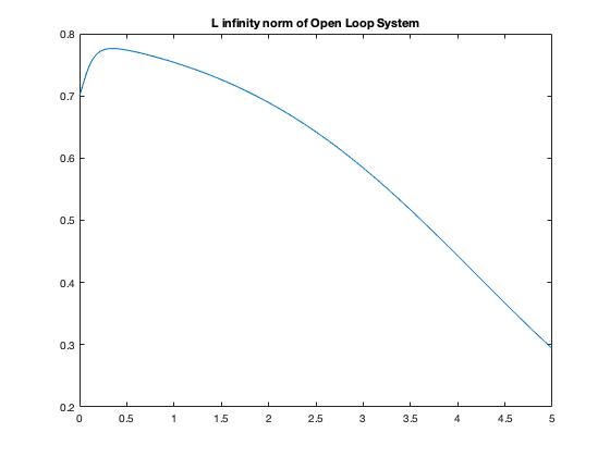
Figure 1: L Infinity Norm of the Open Loop Nonlinear System

The nonlinear system with optimal linear feedback converged when $\zeta_{i}(0)=1$ for $i=0,\ldots,10$ but diverged when $\zeta_{n}(0)=1.1$, see Figure 2.

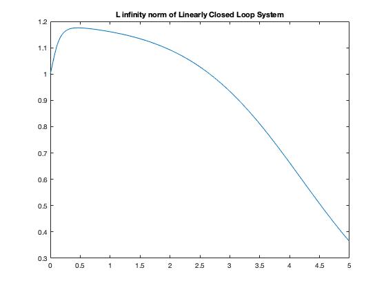
Figure 2: L Infinity Norm of the Nonlinear System using Optimal Linear Feedback

The nonlinear system with optimal linear, quadratic and cubic feedback converged when $\zeta_{i}(0)=4$ for $i=0,\ldots,10$ but diverged when $\zeta_{n}(0)=4.1$, see Figure 3.

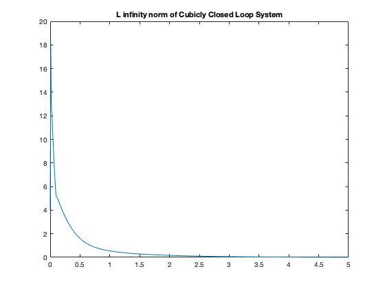
Figure 3: L Infinity Norm of the Nonlinear System using Optimal Linear, Quadratic and Cubic Feedback

VI Conclusion

We have solved the LQR problem for the boundary control of a infinite dimensional system by extending the finite dimensional technique of completing the square. We also optimally locally stabilized a nonlinear reaction diffusion system by extending Al’brekht’s method to infinite dimensions. We showed by example that optimal cubic feedback can lead to a much larger basin of stability than optimal linear feedback. We belive that solving an LQR by the completing the square is applicable to other linear infinite dimensional boundary control problems. We are exploring extending it to the wave equation and the beam equation.

References

[1]
E. G. Al’brekht,
On the Optimal Stabilization of Nonlinear Systems,
PMM-J. Appl. Math. Mech., 25:1254-1266, 1961.
[2]
T. Breiten, K. Kunisch and L. Pfeiffer, Infinite-Horizon Bilinear Optimal Control Problems,
Sensitivity Analysis and Polynomial Feedback Laws, SICON 56:3184-3214, 2018.
[3]
T. Breiten, K. Kunisch and L. Pfeiffer, Feedback Stabilization of the Two-Dimensional Navier-Stokes Equation
by Value Function Approximation, Applied Mathematics and Optimization, 80:599-641, 2019.
[4]
J. Burns and K. Hulsing, Numerical methods for approximating functional gains in LQR boundary control problems,
Mathematical and Computer Modelling 33:89-100, 2001.
[5]
J. Burns and B. King, Representation of feedback operators for hyperbolic systems, Computation and Control IV,
pp. 57-73, Springer 1995.
[6]
J. Burns, D. Rubio and B. King, Regularity of feedback operators for boundary control of thermal processes,
in the Proceedings of the First international conference on nonlinear problems in aviation and aerospace, 1994.
[7]
J. Crank and P. Nicolson, A practical method for numerical evaluation of solutions of partial differential equations of the heat conduction type
Proc. Camb. Phil. Soc. 43, pp. 50-67, 1947.
[8]
R. Curtain and H. Zwart, An Introduction to Infinite-Dimensional Linear Systems Theory, Springer-Verlag, 1995.
[9]
R. Curtain and H. Zwart, Introduction to Infinite-Dimensional Systems Theory, Springer-Verlag, 2020.
[10]
K. Hulsing, Numerical Methods for Approximating Functional Gains for LQR Control of Partial Differential Equations, PhD Thesis,
Department of Mathematics, Virginia Tech, 1999.
[11]
E. Fernandez-Cara and E. Zuazua, E. Null and approximate
controllability for weakly blowing up semilinear heat equations.
Annales de IIHP, Analyse non Lineaire, 17:583-616, 2000.
[12]
B. King, Representation of feedback operators for parabolic control problems,
Proceedings of the American Mathematical Society, 128:1339-1346, 2000.
[13]
A. J. Krener, Nonlinear Systems Toolbox, available on request from ajkrener@nps.com.
[14]
A. J. Krener, Stochastic HJB Equations and Regular Singular Points, in
Modeling, Stochastic Control, Optimization, and Applications, G. Yin and
Q. Zhang, eds., IMA Volumes in Mathematics and its Applications, Springer
Nature, Switzerland, pages 351-368.
[15]
A. J. Krener, Series Solution of Discrete Time Stochastic Optimal Control
Problems, arXiv : submit/2607143 [math.OC] also in the Proceedings of the
2020 IFAC World Congress.
[16]
A. J. Krener,
Al’brekht’s Method in Infinite Dimensions,
Proceeding of the Conference on Decision and Control, 2020.
[17] M. Krstic and A. Smyshlyaev, Boundary Control of PDEs, SIAM, 2008.
[18]
K. Kunisch and L. Pfeiffer, The Effect of the Terminal Penalty in Receding Horizon Control for a Class of Stabilization Problems,
ESAIM: Control, Optimisation and Calculus of Variations, v. 26, 2020.
[19] J. L. Lions, Optimal Control of Systems Governed by Partial Differential Equations, Springer Verlag, Berlin, 1971.
[20]
C. Navasca, Local solutions of the dynamic programming equations
and the Hamilton Jacobi Bellman PDEs, PhD Thesis, University of
California, Davis, 2002.
[21]
R. Vazquez and M. Krstic,
Control of 1-D parabolic PDEs with Volterra nonlinearities, Part I: Design, Automatica 44:2778-2790, 2008.