Exploring KSZ velocity reconstruction with $N$-body simulations and the halo model

Abstract

KSZ velocity reconstruction is a recently proposed method for mapping the largest-scale modes of the universe, by applying a quadratic estimator ${\hat{v}_{r}}$ to the small-scale CMB and a galaxy catalog. We implement kSZ velocity reconstruction in an $N$-body simulation pipeline and explore its properties. We find that the reconstruction noise can be larger than the analytic prediction which is usually assumed. We revisit the analytic prediction and find additional noise terms which explain the discrepancy. The new terms are obtained from a six-point halo model calculation, and are analogous to the $N^{(1)}$ and $N^{(3/2)}$ biases in CMB lensing. We implement an MCMC pipeline which estimates $f_{NL}$ from $N$-body kSZ simulations, and show that it recovers unbiased estimates of $f_{NL}$, with statistical errors consistent with a Fisher matrix forecast. Overall, these results confirm that kSZ velocity reconstruction will be a powerful probe of cosmology in the near future, but new terms should be included in the noise power spectrum.

I Introduction

The cosmic microwave background (CMB) has been a gold mine of cosmological information. So far, the constraining power of the CMB has come mainly from “primary” anisotropy from the last scattering surface (which dominates at angular wavenumbers $l\lesssim 2000$) and gravitational lensing (which dominates at $2000\lesssim l\lesssim 4000$). On even smaller scales ($l\gtrsim 4000$), the CMB temperature is dominated by the kinetic Sunyaev-Zeldovich (kSZ) effect: Doppler shifting of CMB photons by free electrons in the late universe.

The kSZ effect has been detected in cross-correlation with large-scale structure, with the latest measurements approaching 10$\sigma$ Hand et al. (2012); Planck Collaboration et al. (2016); Schaan et al. (2016); DES/SPT Collaboration et al. (2016); Hill et al. (2016); De Bernardis et al. (2017); Schaan et al. (2020), and upcoming experiments such as Simons Observatory Ade et al. (2019) should make percent-level measurements in the next few years. In anticipation of these upcoming measurements, it is very interesting to ask how best to constrain cosmological parameters with the kSZ effect, possibly in cross-correlation with large-scale structure.

A variety of kSZ-sensitive statistics have been proposed (e.g. Dore et al. (2004); DeDeo et al. (2005); Ho et al. (2009); Hand et al. (2012); Li et al. (2014); Alonso et al. (2016); Smith and Ferraro (2017); Deutsch et al. (2018); Smith et al. (2018) and references therein), but in this paper we focus on the velocity reconstruction estimator ${\hat{v}_{r}}$ from Deutsch et al. (2018). Velocity reconstruction is a particularly convenient kSZ estimator for cosmological applications, since it is straightforward to include ${\hat{v}_{r}}$ in analyses involving multiple large-scale structure fields, or incorporate complications like redshift-space distortions (RSD) Smith et al. (2018).

The kSZ velocity reconstruction ${\hat{v}_{r}}$ is a quadratic estimator which reconstructs the large-scale radial velocity ${\hat{v}_{r}}({\bf k}_{L})$ from small-scale modes of a galaxy field $\delta_{g}({\bf k}_{S})$ and CMB temperature $T({\bf l})$. (For the precise definition, see §V.) The scales involved are roughly $k_{L}\sim 10^{-2}$ Mpc^-1, $k_{S}\sim 1$ Mpc^-1, and $l_{\rm CMB}\sim 5000$. Thus, the underlying signal for the reconstruction is the velocity field on large scales where it can be modelled very accurately, but the reconstruction noise is hard to model, since the noise is derived from nonlinear scales.

KSZ velocity reconstruction is interesting for cosmology because its noise power spectrum is smaller on large scales than previously known methods, such as galaxy surveys, as we will explain in the next few paragraphs. First, we note that on large scales, linear theory is a good approximation, and radial velocity $v_{r}$, velocity $v$, and matter overdensity $\delta_{m}$ are related in Fourier space by:

$$v_{r}({\bf k}_{L})=\mu v({\bf k}_{L})=\mu\frac{faH}{k_{L}}\delta_{m}({\bf k}_{L})$$ (1)

Here, $f=\partial\log D/\partial\log a$ is the usual RSD parameter, and $\mu=k_{Lr}/k_{L}$ is the cosine of the angle between the Fourier mode ${\bf k}_{L}$ and the line of sight. Therefore, by applying appropriate factors of $\mu$ and $(faH/k)$, the radial velocity reconstruction ${\hat{v}_{r}}$ may be viewed as a reconstruction of $v$ or $\delta_{m}$. This allows us to compare the noise power spectrum of kSZ velocity reconstruction to other LSS observables, which measure the density field $\delta_{m}$.

To take a concrete example, consider a galaxy survey, which measures the density field $\delta_{m}$ with a noise power spectrum $N(k)=b_{g}^{-2}n_{g}^{-1}$ which is constant on large scales. The noise power spectrum of the kSZ velocity reconstruction ${\hat{v}_{r}}({\bf k}_{L})$ is more complicated, but for now we just note that $N_{v_{r}}(k_{L})$ is also constant on large scales. (The noise power spectrum $N_{v_{r}}$ will be discussed in depth in §V, §VI.) To compare the two, we convert the kSZ velocity reconstruction to a reconstruction of $\delta_{m}$ using Eq. (1), obtaining noise power spectrum:

$$N_{\delta_{m}}^{\rm kSZ}({\bf k}_{L})=\left(\frac{k_{L}}{\mu faH}\right)^{2}N_{v_{r}}({\bf k}_{L})$$ (2)

Due to the factor $k_{L}^{2}$ on the RHS, the kSZ-derived reconstruction of the large-scale modes has parametrically lower noise than the galaxy field. This low-noise large-reconstruction has several potential applications (e.g. Mueller et al. (2015); Zhang and Johnson (2015); Terrana et al. (2017); Cayuso and Johnson (2020); Hotinli et al. (2019); Contreras et al. (2019)), but we will concentrate on the cosmological parameter $f_{NL}$. In Münchmeyer et al. (2019); Contreras et al. (2019), it was shown that adding kSZ data to an analysis of galaxy clustering can significantly improve $f_{NL}$ constraints, relative to the galaxies alone. In this forecast, the $f_{NL}$ sensitivity arises from non-Gaussian bias Dalal et al. (2008); Slosar et al. (2008) in the galaxy survey. The field $v_{r}$ is not directly sensitive to $f_{NL}$, but including it helps improve the $f_{NL}$ constraint, using the idea of sample variance cancellation Seljak (2009).

Summarizing, kSZ velocity reconstruction estimator is emerging as an interesting new tool for constraining cosmology, using upcoming kSZ and large-scale structure data. However, there is currently a major caveat. As mentioned above, the reconstruction ${\hat{v}_{r}}$ is derived from LSS modes on scales $k_{S}\sim 1$ Mpc^-1, and therefore the reconstruction noise depends on statistics of nonlinear modes which are difficult to model. Forecasting work so far (e.g. Deutsch et al. (2018); Smith et al. (2018); Münchmeyer et al. (2019)) has used simple analytic models which approximate the true statistics of the reconstruction noise. The purpose of this paper is to assess the validity of these approximations, by applying kSZ velocity reconstruction to $N$-body simulations.

In the bullet points below, we separate the issues by dissecting the different approximations which are usually made, and summarize the main results of this paper.

• In Smith et al. (2018) it was argued that the kSZ-derived velocity reconstruction ${\hat{v}_{r}}({\bf k})$ is an estimator of the true radial velocity on large scales:

  $${\hat{v}_{r}}({\bf k})=b_{v}v_{r}^{\rm true}({\bf k})+\mbox{(reconstruction noise)}$$ (3)

  where the reconstruction noise is uncorrelated with $v_{r}^{\rm true}$, and the bias $b_{v}$ is constant on large scales. The value of $b_{v}$ depends on the mismatch between the true small-scale galaxy-electron power spectrum $P_{ge}(k_{S})$ and the fiducial spectrum $P_{ge}^{\rm fid}(k_{S})$ used to construct the quadratic estimator.

  In this paper, we will confirm all of these “map-level” properties of the velocity reconstruction estimator ${\hat{v}_{r}}$ using $N$-body simulations. We also find that, although $b_{v}$ is constant on the largest scales, it starts to acquire scale dependence at a surprisingly small value of $k$ (see Figure 3).

• Moving from “map level” to power spectra, we next consider the power spectrum of the reconstruction noise. In Smith et al. (2018), an analytic model was given for the noise power spectrum, which makes the approximation that the small-scale galaxy field $\delta_{g}({\bf k}_{S})$ and the small-scale CMB $T({\bf l})$ are uncorrelated. This is a good approximation if the CMB modes are noise-dominated, but potentially dubious if the CMB is kSZ-dominated. In this paper, we will denote the reconstruction noise power spectrum computed in this approximation by $N_{v_{r}}^{(0)}({\bf k}_{L})$, and call it the “kSZ $N^{(0)}$-bias”. This terminology is intended to emphasize an analogy with CMB lensing which will be explained later in the paper.

  We compare the reconstruction noise power spectrum in our simulations with the kSZ $N^{(0)}$-bias, and find a significant discrepancy, even in the limit ${\bf k}_{L}\rightarrow 0$. For the fiducial survey parameters used in this paper (see §III), the $N^{(0)}$-bias underpredicts the true reconstruction noise power spectrum by a factor 2–3. This turns out to have a small effect on the bottom-line constraint on $f_{NL}$, but this may not be the case for other choices of survey parameters (CMB noise, galaxy density, redshift, etc.) This result shows that the $N^{(0)}$-bias proposed in Smith et al. (2018) as a model for reconstruction noise is sometimes incomplete.

• Motivated by this discrepancy between theory and simulation, we revisit the calculation of the kSZ reconstruction noise, and find additional terms. The new terms are analogous to the $N^{(1)}$-bias Kesden et al. (2003) and $N^{(3/2)}$-bias Böhm et al. (2016) in CMB lensing, and are obtained from a six-point halo model calculation. We calculate the new terms under some simplifying approximations, and find that they explain the excess noise seen in simulations (see Figure 6). The new terms are algebraically simple enough that including them in future forecasts or data analysis should be straightforward (see Eq. (81)).

• Moving from the reconstruction noise power spectrum to higher-point statistics, we next study the question of whether reconstruction noise is a Gaussian field. As a simple test for Gaussianity, we compute the correlation matrix between $k$-bands of the estimated reconstruction noise power spectrum (which would be the identity matrix for a Gaussian field). The bandpower covariance determines statistical errors on parameters derived from power spectra. In particular, the $f_{NL}$ Fisher matrix forecasts from Münchmeyer et al. (2019) implicitly assume that bandpower correlations are small, and we would like to test this assumption.

  In simulation, we find that bandpower correlations are small on the very large scales which dominate $f_{NL}$ constraints, but increase rapidly with $k$, and become order-one at $k\sim 0.03$ Mpc^-1.

• Putting everything together, we develop an “end-to-end” pipeline which recovers $f_{NL}$ from a simulated galaxy catalog and kSZ map. The pipeline applies the quadratic estimator ${\hat{v}_{r}}$, then performs MCMC exploration of the posterior likelihood for parameters $(f_{NL},b_{g},b_{v})$, given realizations of the galaxy field $\delta_{g}$ and velocity reconstruction ${\hat{v}_{r}}$. When deriving the posterior likelihood, we assume that the reconstruction noise power spectrum is equal to the $N^{(0)}$-bias, and that the reconstruction noise is a Gaussian field. Based on previous bullet points, these approximations are imperfect, but their impact on parameter constraints should be small, and therefore it seems plausible that the posterior likelihood will produce valid parameter constraints.

  We find that kSZ velocity reconstruction works! We run the pipeline on simulations with both zero and nonzero $f_{NL}$, in a noise regime where sample variance cancellation is important, and demonstrate that it recovers unbiased $f_{NL}$ estimates, with statistical errors consistent with Fisher matrix forecasts.

These results largely serve as zeroth-order validation of the basic kSZ velocity reconstruction framework from Deutsch et al. (2018); Smith et al. (2018) and $f_{NL}$ forecasts from Münchmeyer et al. (2019), with the addition of new terms in the reconstruction noise. This initial exploratory study can be extended in several interesting directions; see §VIII for systematic discussion.

To test kSZ velocity reconstruction as accurately as possible, we want to use as much simulation volume as we can. For this reason, we use collisionless $N$-body simulations, which have much lower computational cost per unit volume than hydrodynamical simulations. We approximate the electron overdensity field by the dark matter field ($\delta_{e}=\delta_{m}$), and approximate the galaxy catalog by a halo catalog ($\delta_{g}=\delta_{h}$). These are crude approximations, and in particular our approximation $\delta_{e}=\delta_{m}$ means that we overpredict the galaxy-electron power spectrum $P_{ge}(k_{S})$ by an order-one factor. However, in this paper our goal is to compare theory and simulation, and the level of agreement is unlikely to depend on details of small-scale power spectra, as long as the analysis is self-consistent. Since we use collisionless simulations, we can also leverage the high-resolution Quijote public simulations Villaescusa-Navarro et al. (2019) with a total volume of 100 Gpc³ and $f_{NL}=0$. For $f_{NL}\neq 0$, we run GADGET-2 Springel (2005) with a custom initial condition generator.

This paper builds on previous papers which explore the effects of primordial non-Gaussianity in $N$-body simulations, e.g. Dalal et al. (2008); Desjacques et al. (2009); Pillepich et al. (2010); Grossi et al. (2009); Giannantonio and Porciani (2010); Wagner and Verde (2012); Hamaus et al. (2011); Scoccimarro et al. (2012); Baldauf et al. (2016); Biagetti et al. (2017) and references therein. The new ingredient is the kSZ velocity reconstruction ${\hat{v}_{r}}$. To our knowledge, there is only one previous paper which explores kSZ velocity reconstruction in simulations Cayuso et al. (2018). There, a large correlation was found between the reconstructed radial velocity ${\hat{v}_{r}}$ and the true radial velocity $v_{r}^{\rm true}$, but the reconstruction noise was not compared with theory, and non-Gaussian simulations were not studied.

This paper is organized as follows. In §III, we describe our simulation pipeline for generating large-scale structure and kSZ realizations. In §IV, we show large-scale structure and CMB power spectra from our simulations. In §V, we study the kSZ velocity reconstruction estimator ${\hat{v}_{r}}$ in detail, and characterize key properties such as bias, noise, and non-Gaussian bandpower covariance. In §VI, we calculate kSZ reconstruction noise in the halo model, and find new terms $N^{(1)}$ and $N^{(3/2)}$ which agree with the simulations. We present our MCMC-based $f_{NL}$ pipeline in §VII, and conclude in §VIII. The code for this work can be accessed at https://github.com/utkarshgiri/kineticsz.

II Preliminaries and notation

II.1 “Snapshot” geometry

Following Smith et al. (2018), we use the following simplified “snapshot” geometry throughout the paper. We take the universe to be a periodic 3-d box with comoving side length $L=1$ $h^{-1}$ Gpc and volume $V=L^{3}$, “snapshotted” at redshift $z_{*}=2$, corresponding to comoving distance $\chi_{*}\approx 5200$ Mpc. The notation $(\cdot)_{*}$ means “evaluated at redshift $z_{*}$”, e.g. $H_{*}$ is the Hubble expansion rate at $z_{*}$, and $\chi_{*}$ is comoving distance between $z=0$ and $z=z_{*}$.

Three-dimensional large-scale structure fields, such as the galaxy overdensity $\delta_{g}({\bf x})$, are defined on a 3-d periodic box of comoving side length $L$. Two-dimensional angular fields, such as the CMB $T({\boldsymbol{\theta}})$, are defined on a 2-d periodic flat sky with angular side length $L/\chi_{*}$. We define line-of-sight integration by projecting the 3-d box onto the xy-face of the cube, with a factor $1/\chi_{*}$ to convert from spatial to angular coordinates. We denote transverse coordinates of the box by $(x,y)$, but denote the radial coordinate by $r$ (not $z$, to avoid notational confusion with redshift). We denote a unit three-vector in the radial direction by ${\bf\hat{r}}$, and denote the transverse part of a three-vector ${\bf x}$ by ${\bf x}_{\perp}$. Thus a galaxy at spatial location ${\bf x}$ appears at angular sky location ${\boldsymbol{\theta}}={\bf x}_{\perp}/\chi_{*}$.

In the full lightcone geometry, the kSZ temperature anisotropy is given by a line-of-sight integral $T({\boldsymbol{\theta}})=\int dr\,K(r)\,({\bf\hat{r}}\cdot{\bf q}_{e}({\boldsymbol{\theta}},r))$, where ${\bf q}_{e}=(1+\delta_{e}){\bf v}_{e}$ is the dimensionless electron momentum field, and $K(\cdot)$ is the kSZ radial weight function:

$$K(z)=-T_{\rm CMB}\,\sigma_{T}\,n_{e,0}\,x_{e}(z)\,e^{-\tau(z)}\,(1+z)^{2}$$ (4)

In the snapshot geometry, this line-of-sight integral becomes:

$$T_{\rm kSZ}({\boldsymbol{\theta}})=K_{*}\int_{0}^{L}dr\,\Big{(}{\bf\hat{r}}\cdot{\bf q}_{e}(\chi_{*}{\boldsymbol{\theta}}+r{\bf\hat{r}})\Big{)}$$ (5)

II.2 Fourier conventions

Our Fourier conventions for a 3-d field $f({\bf x})$ with power spectrum $P(k)$ are:

$$f({\bf k})=\int d^{3}{\bf x}\,f({\bf x})e^{-i{\bf k}\cdot{\bf x}}\hskip 28.45274pt\langle f({\bf k})f({\bf k}^{\prime})^{*}\rangle=P(k)(2\pi)^{3}\delta^{3}({\bf k}-{\bf k}^{\prime})$$ (6)

In a finite pixelized 3-d volume $V$, we use Fourier conventions:

$$f({\bf k})=\frac{V}{N_{\rm pix}}\sum_{{\bf x}}f({\bf x})e^{-i{\bf k}\cdot{\bf x}}\hskip 28.45274pt\big{\langle}f({\bf k})f({\bf k}^{\prime})^{*}\big{\rangle}=VP(k)\delta_{{\bf k}{\bf k}^{\prime}}$$ (7)

With these conventions, the radial velocity $v_{r}({\bf k})$ and matter overdensity $\delta_{m}({\bf k})$ are related in linear theory by:

$$v_{r}({\bf k})=ik_{r}\left(\frac{faH}{k^{2}}\right)\delta_{m}({\bf k})$$ (8)

Here, $f(z)=(\partial\log D(z)/\partial\log a)$, where $D(z)$ is the growth function.

Similarly, our Fourier conventions for a 2-d flat-sky field $f({\boldsymbol{\theta}})$ with angular power spectrum $C_{l}$ are:

$$f({\bf l})=\int d^{2}{\boldsymbol{\theta}}\,f({\boldsymbol{\theta}})e^{-i{\bf l}\cdot{\boldsymbol{\theta}}}\hskip 28.45274pt\big{\langle}f({\bf l})f({\bf l}^{\prime})^{*}\big{\rangle}=C_{l}(2\pi)^{2}\delta^{2}({\bf l}-{\bf l}^{\prime})$$ (9)

In finite pixelized 2-d area $A$ this becomes:

$$f({\bf l})=\frac{A}{N_{\rm pix}}\sum_{{\boldsymbol{\theta}}}f({\boldsymbol{\theta}})e^{-i{\bf l}\cdot{\boldsymbol{\theta}}}\hskip 28.45274pt\big{\langle}f({\bf l})f({\bf l}^{\prime})^{*}\big{\rangle}=AC_{l}\delta_{{\bf l}{\bf l}^{\prime}}$$ (10)

In our code, we often represent 2-d fields using dimensionful coordinates ${\bf x}_{\perp}=\chi_{*}{\boldsymbol{\theta}}$ and ${\bf k}_{\perp}={\bf l}/\chi_{*}$, which eliminates factors of $\chi_{*}$ in some equations. For example, the line of sight integral (5) becomes $T({\bf x}_{\perp})=K_{*}\int dr\,({\bf\hat{r}}\cdot q_{e}({\bf x}_{\perp}+r{\bf\hat{r}})$.

II.3 Primordial non-Gaussianity and halo bias

Single-field slow-roll inflation is arguably the simplest model of the early universe. In this model, the initial curvature perturbation $\zeta$ is a Gaussian field to an excellent approximation Acquaviva et al. (2003); Maldacena (2003). This is not the case in many alternative models, and searching for primordial non-Gaussianity (deviations from Gaussian initial conditions) is a powerful probe of physics of the early universe. A wide variety of observationally distinguishable non-Gaussian models has been proposed (see e.g. Akrami et al. (2019) and references therein).

In this paper, we will concentrate on “local-type” non-Gaussianity, in which the initial curvature perturbation $\zeta$ is of the form:

$$\zeta({\bf x})=\zeta_{G}({\bf x})+\frac{3}{5}f_{NL}\big{(}\zeta_{G}({\bf x})^{2}-\langle\zeta_{G}^{2}\rangle\big{)}$$ (11)

where $\zeta_{G}$ is a Gaussian field, and $f_{NL}$ is a cosmological parameter to be constrained from observations. Local-type non-Gaussianity is fairly generic in multifield early universe models, such as curvaton models Linde and Mukhanov (1997); Lyth and Wands (2002); Lyth et al. (2003), or modulated reheating models Dvali et al. (2004); Kofman (2003). Conversely, there are theorems Maldacena (2003); Creminelli and Zaldarriaga (2004) which show that $f_{NL}=0$ in single-field early universe models, i.e. models in which a single field both dominates the stress-energy of the early universe, and determines the initial curvature perturbation.

In a pioneering paper Dalal et al. (2008), Dalal et al showed that large-scale clustering of dark matter halos depends sensitively on $f_{NL}$. More precisely, the halo bias $b_{h}$ is scale dependent on large scales, with functional form:

$$b_{h}(k)=b_{g}+f_{NL}\frac{b_{ng}}{\alpha(k,z)}$$ (12)

where $b_{g}$ is the Gaussian (scale-independent) bias, and:

$$\alpha(k,z)\equiv\frac{2k^{2}T(k)D(z)}{3\Omega_{m}H_{0}^{2}}$$ (13)

The quantity $\alpha(k,z)$ relates the matter overdensity $\delta_{m}({\bf k},z)$ to initial curvature $\zeta({\bf k})$ in linear theory: $\delta_{m}({\bf k},z)=(3/5)\alpha(k,z)\zeta({\bf k})$. On large scales $k\rightarrow 0$, $\alpha(k,z)$ is proportional to $k^{2}$, leading to an $f_{NL}k^{-2}$ term in the halo bias. Thanks to this term, even small values of $f_{NL}$ can produce large observable effects on large scales. Although current large-scale structure constraints on $f_{NL}$ Castorina et al. (2019) are not competitive with CMB constraints Akrami et al. (2019), future LSS experiments which probe large volumes and high redshifts should be comparable or better than the CMB Carbone et al. (2010); de Putter and Doré (2017); Doré et al. (2014); Alonso and Ferreira (2015); Ferraro and Smith (2015); Schmittfull and Seljak (2018).

The parameter $b_{ng}$ in Eq. (12) is given exactly by Slosar et al. (2008); Baldauf et al. (2011):

$$b_{ng}=2\frac{\partial\log n_{h}}{\partial\log\sigma_{8}}$$ (14)

This exact expression is of limited usefulness, since the derivative on the RHS is not an observable quantity. Treating $b_{ng}$ as a free parameter is not a viable option for data analysis, since it would be degenerate with $f_{NL}$ (only the combination $b_{ng}f_{NL}$ would be observable). However, in spherical collapse models of halo formation, $b_{ng}$ is related to the Gaussian bias as:

$$b_{ng}=2\delta_{c}(b_{g}-1)$$ (15)

where $\delta_{c}$ is the collapse threshold, given by $\delta_{c}=1.69$ in the Press-Schechter model Press and Schechter (1974), or $\delta_{c}=1.42$ in Sheth-Tormen Sheth and Tormen (2002). Although Eq. (15) is an approximation to the exact result (14), it is usually accurate at the 10–20% level Desjacques et al. (2009); Pillepich et al. (2010); Grossi et al. (2009); Giannantonio and Porciani (2010); Wagner and Verde (2012); Hamaus et al. (2011); Scoccimarro et al. (2012); Baldauf et al. (2016); Biagetti et al. (2017), and is suitable for data analysis, since the parameters $(b_{g},f_{NL})$ can be jointly constrained without degeneracy.

In our $N$-body simulations, we find that Eq. (15) gives a good fit to the non-Gaussian bias observed in our $N$-body simulations, if the Sheth-Tormen threshold $\delta_{c}=1.42$ is used. (See Figure 1 below.) This is consistent with previous simulation-based studies Pillepich et al. (2010); Grossi et al. (2009); Hamaus et al. (2011); Baldauf et al. (2016), which used the parameterization $b_{ng}=2\sqrt{q}(1.69)(b_{g}-1)$, and found a fudge-factor $\sqrt{q}$ around 0.84 for friends-of-friends halos (which we use in our pipeline, see §III.2). In the rest of the paper, we model large-scale halo bias using Eq. (12), where $b_{ng}$ is given by Eq. (15) with $\delta_{c}=1.42$.

III Simulation pipeline

III.1 Collisionless approximation

Simulating high-fidelity kSZ maps for velocity reconstruction is very computationally challenging. KSZ anisotropy appears on small angular scales in the CMB, where it is sourced by electron density fluctuations on small scales $k_{S}\sim 1$ Mpc^-1, leading to high resolution requirements in a simulation. Furthermore, on these small scales, collisionless $N$-body simulations are not really accurate enough to simulate the electron density, and hydrodynamical simulations should be used instead, which are much more expensive. At the same time, the cosmological constraining power of the kSZ comes from the largest scales, so a large simulation volume is required, if the goal is to make a simulation with an interesting $f_{NL}$ constraint. This combination of volume and resolution requirements presents a serious computational challenge, and new simulation methods are probably required to satisfy all requirements strictly.

In this paper, our goal is simply to test kSZ velocity reconstruction for biases as precisely as possible, under a self-consistent set of assumptions. For this purpose, perfectly accurate kSZ simulations are not required, and approximations are acceptable, as long as they are self-consistent. We will make the approximation that the electron density perfectly traces the dark matter density ($\delta_{e}=\delta_{m}$). This overestimates power spectra such as $P_{ge}$, $P_{ee}$, or $C_{l}^{\rm kSZ}$ by an order-one factor on small scales, since hydrodynamic effects suppress electron fluctuations relative to dark matter Shaw et al. (2012). However, the question of whether kSZ velocity reconstruction is biased is unlikely to depend on the details of these small scale power spectra. For our purposes, what is crucial is that the approximation $\delta_{e}\approx\delta_{m}$ is applied consistently throughout the simulation and reconstruction pipelines.

The approximation $\delta_{e}\approx\delta_{m}$ dramatically decreases computational cost, since we can use collisionless $N$-body simulations. Similarly, instead of simulating galaxies, we use dark matter halos as a proxy for galaxies, i.e. we make the approximation $\delta_{g}\approx\delta_{h}$. In the rest of the paper, we use “galaxies” synonymously with “halos”, and “electrons” synonymously with “dark matter particles”.

III.2 $N$-body simulations

We are interested in collisionless $N$-body simulations for both zero and nonzero $f_{NL}$. For $f_{NL}=0$, rather than running our own simulations from scratch, we use the Quijote simulations Villaescusa-Navarro et al. (2019), a large suite of publicly available $N$-body simulations. We use 100 simulations with $1024^{3}$ particles and volume 1 $h^{-3}$ Gpc³ each.

For $f_{NL}\neq 0$, we generated a limited number of $N$-body simulations by running GADGET-2 Springel (2005) with non-Gaussian initial conditions as follows. We simulate the initial curvature $\zeta$, by simulating a Gaussian field $\zeta_{G}$, and then adding a quadratic term:

$$\zeta({\bf x})=\zeta_{G}({\bf x})+\frac{3}{5}f_{NL}\big{(}\zeta_{G}({\bf x})^{2}-\langle\zeta_{G}^{2}\rangle\big{)}$$ (16)

where the squaring operation is performed in real space. We evolve $\zeta$ to the Newtonian potential $\Phi$ at redshift $z_{\rm ini}=127$, using linear transfer functions computed using CLASS Lesgourgues (2011). We then generate initial conditions for GADGET-2 at $z_{\rm ini}=127$ using the Zeldovich approximation Jeong (2010):

$$\Psi_{i}({\bf q}) =-\partial_{i}\partial^{-2}\delta_{m}({\bf q})=-\frac{2}{3a^{2}H(a)^{2}}\Big{(}\partial_{i}\Phi({\bf q})\Big{)}$$ (17)

$$v_{i}({\bf q}) =\frac{\partial\Psi_{i}}{\partial\tau}=-\frac{2}{3aH(a)}\Big{(}\partial_{i}\Phi({\bf q})\Big{)}$$ (18)

Here, ${\bf q}$ is the initial Lagrangian location of particles which in our case occupy center of 3D mesh, $\Psi_{i}({\bf q})$ is the initial particle displacement, and $v_{i}({\bf q})$ is the initial velocity. We evolve particles from $z_{\rm ini}=127$ to $z_{*}=2$ using GADGET-2 with the same parameters (cosmological parameters, force softening length, etc.) as the Quijote simulations.

III.3 Large-scale structure fields: $\delta_{m}$, $\delta_{h}$, $q_{r}$

The output of an $N$-body simulation is a catalog of particles with velocities. In this section, we describe our postprocessing of the catalog, to obtain pixelized 3-d maps of the matter overdensity $\delta_{m}({\bf x})$, halo overdensity $\delta_{h}({\bf x})$, and radial momentum $q_{r}({\bf x})$.

To compute $\delta_{m}({\bf x})$, we grid particle positions on a regular 3D mesh using the cloud-in-cell (CIC) algorithm Hockney and Eastwood (1981), implemented in the public code nbodykit Hand et al. (2018). We use a 3D mesh with $1024^{3}$ pixels, corresponding to pixel size 1 $h^{-1}$ Mpc.

To obtain a halo catalog, we run the Rockstar halo-finder Behroozi et al. (2013) on the particle positions. (Note that the Quijote simulations include a halo catalog, but we run our own halo finder instead, so that simulations with zero and nonzero $f_{NL}$ are processed consistently.) Rockstar implements a modified version of the Friends-of-Friends (FOF) algorithm Davis et al. (1985). After the halo catalog is produced, it is processed to obtain a halo overdensity map $\delta_{h}({\bf x})$ by CIC-gridding halo positions.

We use an FOF linking length of 0.28 and require a minimum of 40 particles to classify a structure as a halo. This results in halo bias $b_{h}\sim 3.24$ and density $n_{h}^{3d}\approx 2.5\times 10^{-4}\ \mathrm{Mpc^{-3}}$ for simulations with $f_{nl}=0$ at redshift $z_{*}=2$. Since we are using halos as proxies for galaxies, our effective 2-d galaxy number density is $dn_{g}^{2d}/dz=(\chi_{*}^{2}/H_{*})n_{h}^{3d}=0.8$ arcmin^-2. In comparison, DESI has a combined (ELG+LRG+QSO) number density $dn_{g}^{2d}/dz=0.91$ arcmin^-2 at its peak at $z=0.75$ DESI Collaboration et al. (2016), while Vera Rubin Observatory “gold” sample will have a number density $dn_{g}^{2d}/dz=36$ arcmin^-2 at its peak at $z=0.6$ LSST Science Collaboration et al. (2009).

The radial momentum field deserves some discussion. We are interested in making 3-d maps of the true radial velocity $v_{r}^{\rm true}$, in order to compare it to the kSZ velocity reconstruction $\hat{v}_{r}$ on large scales. However, in an $N$-body simulation, the definition of $v_{r}^{\rm true}$ is ambiguous. Here are three possibilities:

1. We can use the radial momentum $q_{r}=(1+\delta)v_{r}$. Since momentum is particle-weighted, it can be directly computed from particle positions and velocities.

2. We can use the linear velocity field $v_{r}^{\rm lin}({\bf k})$, obtained by applying linear transfer functions to the initial conditions.

3. We can choose a smoothing scale, and define the velocity to be the smoothed momentum, divided by the smoothed density (appropriately regulated to avoid dividing by zero in voids).

We actually tried all three possibilities, and found that the first (the radial momentum $q_{r}$) has the highest correlation with the kSZ velocity reconstruction $\hat{v}_{r}$. This makes sense intuitively by considering the case of a “near-void” region whose density is close to zero. In a near-void region, the velocity reconstruction $\hat{v}_{r}$ is small, since a factor of the small-scale inhomogeneity $\delta_{g}({\bf k}_{S})$ appears in $\hat{v}_{r}$. Since the momentum $q_{r}$ is also small in a near-void, but the radial velocity $v_{r}$ is not, we expect $\hat{v}_{r}$ to correlate more strongly with $q_{r}$ than with $v_{r}$.

Since $q_{r}$ has the highest correlation with ${\hat{v}_{r}}$, and is also most straightforward to derive from an $N$-body simulation, we will use $q_{r}$ throughout the paper. (In hindsight, it would make sense to rename the quadratic estimator ${\hat{v}_{r}}\rightarrow\hat{q}_{r}$, and call it “kSZ momentum reconstruction” instead of “kSZ velocity reconstruction”. However, we will use the ${\hat{v}_{r}}$ notation and velocity reconstruction terminology, for consistency with previous papers.) With this motivation for introducing the radial momentum, it is straightforward to compute $q_{r}({\bf x})$ from an $N$-body simulation. We simply CIC-grid particles as before, weighting each particle by its radial velocity.

A technical point: we use compensated CIC-gridding with 1024³ pixels throughout our pipeline, even though this suppresses power at wavenumbers close to the Nyquist frequency of the pixelization Hockney and Eastwood (1981); Sefusatti et al. (2016); Hand et al. (2018). The suppression is a 3% at $k=0.8k_{\rm Nyq}$, and 30% at $k=k_{\rm Nyq}$ Hand et al. (2018). In our kSZ velocity reconstruction pipeline, this does not lead to biases, provided that CIC-gridded fields and power spectra are used self-consistently throughout the pipeline. For example, we find (Figure 3 below) that the kSZ velocity reconstruction bias $b_{v}$ is 1 on large scales, if the quadratic estimator ${\hat{v}_{r}}$ is implemented with CIC-gridding, and defined self-consistently using CIC-gridded power spectra $P_{ge}(k_{S}),P_{gg}(k_{S})$ (see Eq. (26)).

III.4 CMB maps

Given the output from an $N$-body simulation, we simulate a kSZ map as follows. Let ${\bf x}_{i}$ denote the 3-d position of the $i$-th particle in the simulation (where $i=1,\cdots,N_{\rm part}$), let ${\bf v}_{i}$ denote the velocity, and let ${\boldsymbol{\theta}}_{i}={\bf x}_{\perp i}/\chi_{*}$ denote the projected angular sky location. We approximate the momentum ${\bf q}({\bf x})$ as a sum of velocity-weighted delta functions:

$${\bf q}({\bf x})=\frac{1}{n_{p}}\sum_{i}{\bf v}_{i}\delta^{3}({\bf x}-{\bf x}_{i})$$ (19)

where $n_{p}=N_{\rm part}/L_{\rm box}^{3}$ is the 3-d particle number density. Plugging into the line-of-sight integral (Eq. (5)), the kSZ temperature is:

$$T_{\rm kSZ}({\boldsymbol{\theta}})=\frac{K_{*}}{\chi_{*}^{2}n_{p}}\sum_{i}({\bf\hat{r}}\cdot{\bf v}_{i})\delta^{2}({\boldsymbol{\theta}}-{\boldsymbol{\theta}}_{i})$$ (20)

In our pipeline, we discretize CMB maps using $(1024)^{2}$ pixels, corresponding to angular pixel size $(\Delta\theta)=L_{\rm box}/(1024\chi_{*})=0.96$ arcmin, and Nyquist frequency $l_{\rm Nyq}=\pi/(\Delta\theta)=11250$. We evaluate the RHS of Eq. (20) by gridding each delta function onto the 2-d mesh using the Cloud-in-Cell (CIC) scheme Hockney and Eastwood (1981).

We add simulations of the lensed primary CMB and instrumental noise to our simulations, treating both contributions as Gaussian fields. We use noise power spectrum:

$$N_{l}=s_{w}^{2}\exp\left[\frac{l(l+1)\theta_{\rm fwhm}^{2}}{8\ln 2}\right]$$ (21)

with white noise level $s_{w}=0.5$ $\mu$K-arcmin, and beam size $\theta_{\rm fwhm}=1$ arcmin. Note that we treat the non-kSZ CMB as Gaussian, which neglects possible biases from non-Gaussian secondaries. This is a loose end, although symmetry arguments suggest that biases are probably small. For more discussion, see §VIII.

In the rest of the paper, we fix fiducial survey parameters described above ($s_{w}=0.5$ $\mu$K-arcmin, $\theta_{\rm fwhm}=1$ arcmin, $b_{g}=3.24$, effective $dn_{g}/dz=0.8$ arcmin^-2). Our galaxy survey parameters are similar to DESI, and our CMB parameters are intentionally futuristic (a bit better than CMB-S4), in order to maximize statistical power of our simulations.

IV LSS and CMB power spectra

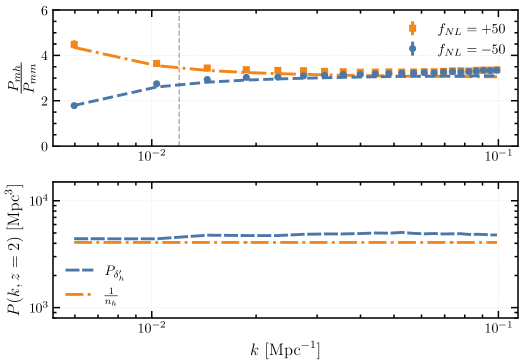
Figure 1: Top panel. Large-scale halo bias $b_{h}(k)=P_{mh}(k)/P_{mm}(k)$ from $N$-body simulations with $f_{NL}=\pm 50$. For comparison, we show the bias model (22), with $b_{g}=3.01$, $3.15$ for $f_{NL}=-50$, $50$ respectively. (These values were obtained from the MCMC pipeline to be presented in §VII.) For each value of $f_{NL}$, we use four $N$-body simulations with volume 1 $h^{-3}$ Gpc³ each. Bottom panel. Halo shot noise from simulation from the same set of simulations, defined as the power spectrum of the field $\delta_{h}^{\prime}({\bf k})=\delta_{m}({\bf k})-b_{h}(k)\delta_{m}({\bf k})$, compared to the Poisson prediction $P_{\delta_{h}^{\prime}}(k)=1/n_{h}$.

In this section we present matter, halo, and CMB power spectra from our simulation pipeline. In the next section we will study higher-point statistics and kSZ velocity reconstruction. We start by confirming that the large-scale halo bias is described by the model:

$$b_{h}(k)=b_{g}+f_{NL}\frac{2\delta_{c}(b_{g}-1)}{\alpha(k,z)}\hskip 28.45274pt(\delta_{c}=1.42)$$ (22)

in agreement with previous studies Dalal et al. (2008); Desjacques et al. (2009); Pillepich et al. (2010); Grossi et al. (2009); Giannantonio and Porciani (2010); Wagner and Verde (2012); Scoccimarro et al. (2012); Biagetti et al. (2017). In Figure 1 (top), we estimate the halo bias $b_{h}(k)=P_{mh}(k)/P_{mm}(k)$ directly from the matter-halo and matter-matter power spectra of simulations with $f_{NL}=\pm 50$, and find good agreement with the bias model in Eq. (22).

Next we consider the halo-halo power spectrum $P_{hh}(k)$. On large scales, we want to check that linear halo bias plus shot noise is a good description, i.e.

$$P_{hh}(k)=b_{h}(k)^{2}P_{mm}(k)+\frac{1}{n_{h}}$$ (23)

A stronger version of this check is to show that the power spectrum of the field $\delta_{h}^{\prime}=\delta_{h}-b_{h}(k)\delta_{m}$ is consistent with pure shot noise: $P_{\delta_{h}^{\prime}\delta_{h}^{\prime}}(k)=1/n_{h}$. In Figure 1 (bottom), we find good agreement, thus confirming the model (23).

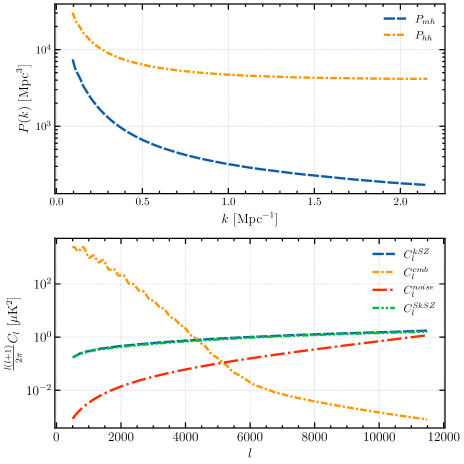
Figure 2: Top. Small scale halo-halo and matter-halo power spectrum from Quijote N-body simulations. These power spectra are used in the definition of the velocity reconstruction estimator ${\hat{v}_{r}}$ (Eq. (26) below). Bottom. Plot showing various contributions to the CMB power spectrum. The lensed CMB power spectrum is computed using the CLASS Boltzmann code Blas et al. (2011), and the noise power spectrum is based on Eq. (21) with $s_{w}=0.5$ $\mu$K-arcmin and $\theta_{\rm fwhm}=1$ arcmin. The kSZ power spectrum $C_{l}^{\rm kSZ}$ is estimated directly from our simulation pipeline. For comparison, we also show the “standard” analytical estimate $C_{l}^{SkSZ}$, based on Shaw et al. (2012) and computed using Eq. (24).

Taken together, Eqs. (22), (23) are a complete model for halo clustering on large scales. Turning next to small scales, we present small-scale power spectra which are relevant for kSZ velocity reconstruction. The definition of the kSZ velocity reconstruction estimator ${\hat{v}_{r}}$ (Eq. (25) below) involves the small-scale galaxy-electron and galaxy-galaxy power spectra $P_{ge}(k_{S}),P_{gg}(k_{S})$, evaluated at wavenumbers $k_{S}\sim 1$ Mpc^-1. In the collisionless $N$-body approximation used in this paper ($\delta_{e}\approx\delta_{m}$, $\delta_{g}\approx\delta_{h})$, these power spectra are equal to $P_{mh}(k_{S})$ and $P_{hh}(k_{S})$, which we show for reference in the top panel of Figure 2.

The definition of ${\hat{v}_{r}}$ also involves the small-scale CMB power spectrum $C_{l}^{\rm tot}$, which is the sum of kSZ, noise, and lensed CMB contributions. These contributions are shown in the bottom panel of Figure 2. The kSZ contribution $C_{l}^{kSZ}$ is estimated directly from the simulations.

As another check on our pipeline, in Figure 2 we compare $C_{l}^{kSZ}$ to the “standard” analytic estimate $C_{l}^{SkSZ}$, and find good agreement. The analytic estimate is derived following Jaffe and Kamionkowski (1998); Shaw et al. (2012) by approximating the electron momentum as ${\bf q}_{e}=(1+\delta_{e}){\bf v}$ where the linear velocity ${\bf v}$ and nonlinear electron field $\delta_{e}$ are Gaussian. In this approximation, the kSZ power spectrum is:

$$C_{l}^{SkSZ}=\frac{(faH_{*})^{2}K_{*}^{2}L}{2}\int\frac{d^{3}{\bf k}^{\prime}}{(2\pi)^{3}}P^{NL}_{mm}(|{\bf k}-{\bf k}^{\prime}|)P_{mm}(k^{\prime})\left.\frac{k(k-2k^{\prime}\mu)(1-\mu^{2})}{k^{\prime 2}(k^{2}+k^{\prime 2}-2kk^{\prime}\mu)}\right|_{\begin{subarray}{c}{\bf k}={\bf l}/\chi_{*}\\ \mu=\hat{\bf k}\cdot\hat{\bf k}^{\prime}\end{subarray}}$$ (24)

where $P_{mm}$ and $P^{NL}_{mm}$ are the linear and non-linear matter power spectrum, and $L$ is the box size.

The kSZ power spectrum in Figure 2 underestimates the predicted $C_{l}$ from hydrodynamical simulations (e.g. Sehgal et al. (2010)) by a factor $\sim$2. This is because our “snapshot” geometry only includes kSZ fluctuations from a redshift slice of thickness $L_{\rm box}=1$ $h^{-1}$ Gpc. (We also make the approximation that electrons trace dark matter, i.e. $P_{ee}\approx P_{mm}$, which has the opposite effect of increasing $C_{l}$, but this is a smaller effect.) This is not an issue for purposes of this paper, where our goal is to test kSZ velocity reconstruction for biases as precisely as possible, under a self-consistent set of assumptions. We considered making the simulations more realistic, by adding simulated kSZ outside the simulated redshift range, but we expect that this would be nearly equivalent to adding uncorrelated Gaussian noise, and would only serve to decrease the precision of our tests.

V The KSZ quadratic estimator applied to $N$-body simulations

V.1 KSZ quadratic estimator

In this section, we describe our implementation of the kSZ velocity reconstruction estimator ${\hat{v}_{r}}$. The inputs to kSZ velocity reconstruction are the 2-d CMB map $T({\bf l})$ and 3-d galaxy overdensity field $\delta_{g}({\bf k})$. The outputs are the 3-d radial velocity reconstruction ${\hat{v}_{r}}({\bf k})$ and noise power spectrum $N_{v_{r}}^{(0)}({\bf k}_{L})$. These are given by Smith et al. (2018):

$${\hat{v}_{r}}({\bf k}_{L}) = N_{v_{r}}^{(0)}({\bf k}_{L})\frac{K_{*}}{\chi_{*}^{2}}\int\frac{d^{3}{\bf k}_{S}}{(2\pi)^{3}}\,\frac{d^{2}{\bf l}}{(2\pi)^{2}}\frac{P_{ge}(k_{S})}{P_{gg}(k_{S})C_{l}^{\rm tot}}\delta_{g}^{*}({\bf k}_{S})T^{*}({\bf l})\,(2\pi)^{3}\delta^{3}\left({\bf k}_{L}+{\bf k}_{S}+\frac{{\bf l}}{\chi_{*}}\right)$$ (25)

$$N_{v_{r}}^{(0)}({\bf k}_{L}) = \frac{\chi_{*}^{4}}{K_{*}^{2}}\left[\int\frac{d^{3}{\bf k}_{S}}{(2\pi)^{3}}\,\frac{d^{2}{\bf l}}{(2\pi)^{2}}\,\frac{P_{ge}(k_{S})^{2}}{P_{gg}(k_{S})C_{l}^{\rm tot}}(2\pi)^{3}\delta^{3}\left({\bf k}_{L}+{\bf k}_{S}+\frac{{\bf l}}{\chi_{*}}\right)\right]^{-1}$$ (26)

The noise power spectrum in the second line (26) is obtained by calculating the two-point function $\langle{\hat{v}_{r}}({\bf k}_{L}){\hat{v}_{r}}({\bf k}_{L}^{\prime})^{*}\rangle$, under the approximation that the galaxy catalog and CMB are independent. To emphasize an analogy with CMB lens reconstruction that will be explained in §VI, we will call the noise power spectrum defined in Eq. (26) the “kSZ $N^{(0)}$-bias” throughout the paper. One of our goals is to compare the kSZ $N^{(0)}$ bias to the reconstruction noise in $N$-body simulations, to test the accuracy of the approximation leading to Eq. (26).

In principle, $N_{v_{r}}^{(0)}({\bf k}_{L})$ is a function of both $k_{L}=|{\bf k}_{L}|$, and the direction of ${\bf k}_{L}$ relative to the line of sight. However, on the large scales which are relevant for constraining $f_{NL}$, it approaches a constant:

$$N_{v_{r}}^{(0)}({\bf k}_{L})\rightarrow\frac{\chi_{*}^{4}}{K_{*}^{2}}\left[\int\frac{d^{2}{\bf l}}{(2\pi)^{2}}\frac{P_{ge}(l/\chi_{*})^{2}}{P_{gg}(l/\chi_{*})C_{l}^{\rm tot}}\right]^{-1}\hskip 28.45274pt({\bf k}_{L}\rightarrow 0)$$ (27)

In Eqs. (25), (26), we have given Fourier-space expressions for ${\hat{v}_{r}}({\bf k}_{L})$ and $N_{v_{r}}^{(0)}({\bf k}_{L})$. These expressions are computationally expensive, and in practice alternative expressions are used, which factorize the computation into FFT’s as follows. The velocity reconstruction ${\hat{v}_{r}}({\bf k}_{L})$ is computed as:

$${\hat{v}_{r}}({\bf k}_{L})=N_{v_{r}}^{(0)}({\bf k}_{L})\frac{K_{*}}{\chi_{*}^{2}}\int d^{3}{\bf x}\,{\tilde{\delta}}_{g}({\bf x})\,{\tilde{T}}\Big{(}\frac{{\bf x}_{\perp}}{\chi_{*}}\Big{)}e^{-i{\bf k}_{L}\cdot{\bf x}}$$ (28)

where the filtered galaxy field ${\tilde{\delta}}_{g}({\bf x})$ and filtered CMB ${\tilde{T}}({\boldsymbol{\theta}})$ are defined by:

$${\tilde{\delta}}_{g}({\bf x})=\int\frac{d^{3}{\bf k}_{S}}{(2\pi)^{3}}\,\frac{P_{ge}({\bf k}_{S})}{P_{gg}({\bf k}_{S})}\delta_{g}({\bf k}_{S})e^{i{\bf k}_{S}\cdot{\bf x}}\hskip 28.45274pt{\tilde{T}}({\boldsymbol{\theta}})=\int\frac{d^{2}{\bf l}}{(2\pi)^{2}}\,\frac{1}{C_{l}^{\rm tot}}T({\bf l})e^{i{\bf l}\cdot{\boldsymbol{\theta}}}$$ (29)

Similarly, the kSZ $N^{(0)}$-bias is computed efficiently as:

$$N_{v_{r}}^{(0)}({\bf k}_{L})=\frac{\chi_{*}^{4}}{K_{*}^{2}}\left[\int d^{3}{\bf x}\,f_{1}({\bf x})\,f_{2}\Big{(}\frac{{\bf x}_{\perp}}{\chi_{*}}\Big{)}e^{-i{\bf k}_{L}\cdot{\bf x}}\right]^{-1}$$ (30)

where the 3-d field $f_{1}$ and 2-d field $f_{2}$ are defined as:

$$f_{1}({\bf x})=\int\frac{d^{3}{\bf k}_{S}}{(2\pi)^{3}}\,\frac{P_{ge}(k_{S})^{2}}{P_{gg}(k_{S})}e^{i{\bf k}_{S}\cdot{\bf x}}\hskip 28.45274ptf_{2}({\boldsymbol{\theta}})=\int\frac{d^{2}{\bf l}}{(2\pi)^{2}}\,\frac{1}{C_{l}^{\rm tot}}\,e^{i{\bf l}\cdot{\boldsymbol{\theta}}}$$ (31)

Eqs. (28), (30) for ${\hat{v}_{r}}$ and $N_{v_{r}}^{(0)}$ are mathematically equivalent to Eqs. (25), (26), but have much lower computational cost.

One more detail of our ${\hat{v}_{r}}$ implementation. The definitions of ${\hat{v}_{r}}$ and $N_{v_{r}}^{(0)}$ above involve small-scale power spectra $P_{ge}(k_{S})$, $P_{gg}(k_{S})$, and $C_{l}^{\rm tot}$. In this paper, we do not attempt to model these small-scale spectra (e.g. with the halo model). Instead, we measure them directly from simulation, by estimating each power spectrum in bandpowers, and interpolating to get a smooth function of wavenumber. The estimated power spectra $P_{ge}(k_{S})$, $P_{gg}(k_{S})$, and $C_{l}^{\rm tot}$ in our simulations were shown previously in Figure 2.

By estimating small-scale power spectra directly from simulation, our pipeline is “cheating”, since $P_{ge}(k_{S})$ is not observable. (The other two small-scale power spectra $P_{gg}(k_{S})$ and $C_{l}^{\rm tot}$ can be estimated directly from data in a real experiment, and so it is not cheating to measure them from simulations.) In a real experiment, we would need to use a fiducial model $P_{ge}^{\rm fid}(k_{S})$, which need not equal the true power spectrum $P_{ge}^{\rm true}(k_{S})$. In Smith et al. (2018), it is predicted that in this situation, the velocity reconstruction acquires a large-scale linear bias:

$${\hat{v}_{r}}({\bf k}_{L})=b_{v}v_{r}({\bf k}_{L})+(\mbox{Reconstruction noise})$$ (32)

where the velocity reconstruction bias $b_{v}$ is $1$ if $P_{ge}^{\rm fid}=P_{ge}^{\rm true}$, but can differ from 1 if $P_{ge}^{\rm fid}\neq P_{ge}^{\rm true}$. We will test this prediction in the next section.

V.2 Noise and bias of velocity reconstruction

In Smith et al. (2018) we predicted that the velocity reconstruction estimator ${\hat{v}_{r}}({\bf k}_{L})$ is an unbiased estimator of the radial momentum $q_{r}({\bf k}_{L})$ on large scales, and that the reconstruction noise is given by the $N^{(0)}$-bias in Eq. (26). These statements are “predictions” since they are derived using analytic approximations to the statistics of large-scale structure on nonlinear scales. In this section, we will test these key predictions with $N$-body simulations.

We start by stating precisely the predictions we would like to test. We define the kSZ velocity reconstruction bias $b_{v}({\bf k}_{L})$ of the simulation by:

$$b_{v}({\bf k}_{L})=\frac{P_{q_{r}{\hat{v}_{r}}}({\bf k}_{L})}{P_{q_{r}q_{r}}({\bf k}_{L})}$$ (33)

Then we predict that $b_{v}\rightarrow 1$ on large scales, if we assume that the galaxy-electron power spectrum $P_{ge}(k_{S})$ is known in advance and used in the quadratic estimator (25). If fiducial power spectrum $P_{ge}^{\rm fid}(k_{S})\neq P_{ge}^{\rm true}(k_{S})$ is used, then we make the weaker prediction that $b_{v}$ approaches a constant on large scales.

We define the reconstruction noise field $\eta({\bf k}_{L})={\hat{v}_{r}}({\bf k}_{L})-b_{v}({\bf k}_{L})q_{r}({\bf k}_{L})$, or equivalently:

$${\hat{v}_{r}}({\bf k}_{L})=b_{v}({\bf k}_{L})q_{r}({\bf k}_{L})+\eta({\bf k}_{L})\hskip 28.45274pt\mbox{where }P_{\eta q_{r}}({\bf k}_{L})=0$$ (34)

Then we predict that the power spectrum $P_{\eta}({\bf k}_{L})$ is equal to the kSZ $N^{(0)}$-bias $N_{v_{r}}^{(0)}({\bf k}_{L})$ given previously in Eq. (26).

Note that in the above, we compare ${\hat{v}_{r}}$ to the radial momentum $q_{r}$, since ${\hat{v}_{r}}$ is expected to be more correlated with momentum than with other definitions of the radial velocity, and momentum is also more straightforward to define in simulation (see discussion in §III.3).

In the rest of this section, we will test the above predictions with simulations. All results in this section use 100 Quijote simulations with $f_{NL}=0$ and total volume 100 $h^{-3}$ Gpc³.

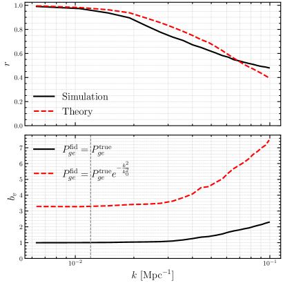
Figure 3: Top panel. Correlation coefficient $r$ between fields ${\hat{v}_{r}}$ and $q_{r}$, where ${\hat{v}_{r}}$ is the kSZ velocity reconstruction derived from an $N$-body simulation, and $q_{r}$ is the true radial momentum of the simulation. We estimate $r$ in $k$-bins using Eq. (35), excluding wavenumbers with $\mu=0$. The “theory” curve was obtained using Eq. (36). Bottom panel. KSZ velocity reconstruction bias $b_{v}$, estimated in $k$-bins using Eq. (37). The solid line was computed assuming perfect knowledge of the galaxy-electron power spectrum $P_{ge}(k_{S})$ in the definition of ${\hat{v}_{r}}$. The dashed line was computed using fiducial galaxy-electron power spectrum $P_{ge}^{\rm fid}(k_{S})=P_{ge}^{\rm true}(k_{S})\exp(-k^{2}/k_{0}^{2})$, where $k_{0}=1$ Mpc^-1. The vertical line at $k=0.012$ Mpc^-1 is the $k_{max}$ that we use in our MCMC pipeline later (§VII).

Before exploring bias and reconstruction noise, we do a simple intuitive comparison between the radial momentum $q_{r}$ and the reconstruction ${\hat{v}_{r}}$. In Figure 3 (top) we show the correlation coefficient between $q_{r}$ and ${\hat{v}_{r}}$. More precisely, we choose a set of $k$-bins, and for each $k$-bin $b$ we define a correlation coefficient $r_{b}^{\rm sim}$ by:

$$r_{b}^{\rm sim}=\frac{\sum_{{\bf k}\in b}{\hat{v}_{r}}^{*}({\bf k})q_{r}({\bf k})}{\left(\sum_{{\bf k}\in b}|q_{r}({\bf k})|^{2}\right)^{1/2}\left(\sum_{{\bf k}\in b}|{\hat{v}_{r}}({\bf k})|^{2}\right)^{1/2}}$$ (35)

It is seen that the kSZ-derived velocity reconstruction ${\hat{v}_{r}}({\bf k})$ is nearly 100% correlated to the true momentum on large scales. This is crucial, since we want to use velocity reconstruction to cancel sample variance in the galaxy field and constrain $f_{NL}$, which requires a high correlation. To quantify this better, we compare to the “theory” prediction for the correlation coefficient:

$$r_{b}^{\rm theory}=\left(\frac{\sum_{{\bf k}\in b}\mu_{{\bf k}}^{2}P_{vv}(k)}{\sum_{{\bf k}\in b}(\mu_{{\bf k}}^{2}P_{vv}(k)+N_{v_{r}}({\bf k}))}\right)^{1/2}$$ (36)

where $\mu_{{\bf k}}=({\bf\hat{k}}\cdot{\bf\hat{r}})$ as usual. This expression for $r_{b}^{\rm theory}$ was calculated assuming $b_{v}=1$ and $P_{\eta}=N_{v_{r}}^{(0)}$.

In Figure 3 (top), the correlation coefficient seen in simulation qualitatively agrees with the theory prediction, but we do see some level of mismatch. On large scales, $r_{b}^{\rm sim}$ is a little smaller than $r_{b}^{\rm theory}$. This is consistent with a factor 2–3 increase in reconstruction noise that we will describe shortly. Intriguingly, on small scales, $r_{b}^{\rm sim}$ is a little larger than $r_{b}^{\rm theory}$. By comparing Figs 3 (bottom) and 4, this can be interpreted as arising from enhancement of the velocity bias $b_{v}$ on small scales, with no corresponding enhancement in reconstruction noise.

Next we would like to test the prediction that the velocity reconstruction bias $b_{v}\rightarrow 1$ on large scales. In Figure 3 (bottom), we show the bias from $N$-body simulations, estimated in non-overlapping $k$-bins by defining:

$$(b_{v})_{b}=\frac{\sum_{{\bf k}\in b}q_{r}({\bf k})^{*}\,{\hat{v}_{r}}({\bf k})}{\sum_{{\bf k}\in b}|q_{r}({\bf k})|^{2}}$$ (37)

for each $k$-bin $b$. The bias is 1 on large scales as predicted. As $k$ increases, the bias is an increasing function of $k$, and becomes large for surprisingly small values of $k$. For example, $b_{v}\approx 2.4$ at $k=0.1$ Mpc^-1. The level of scale dependence seen in the velocity bias $b_{v}(k)$ is much higher than the familiar case of halo bias (see Fig. 1). However, on the very large scales $(k\lesssim 0.01$) that are important for $f_{NL}$ constraints, $b_{v}$ is constant to an excellent approximation.

In Figure 3 (bottom), we also show the velocity bias $b_{v}$ if we construct the quadratic estimator ${\hat{v}_{r}}$ using fiducial galaxy-electron power spectrum $P_{ge}^{\rm fid}(k_{S})\neq P_{ge}^{\rm true}(k_{S})$. For illustrative purposes, we have arbitrary chosen $P_{ge}^{\rm fid}(k_{S})=P_{ge}^{\rm true}(k_{S})\exp(-k^{2}/k_{0}^{2})$, where $k_{0}=1$ Mpc^-1. As predicted, we find that $b_{v}$ approaches a constant on large scales, but the value is $\neq 1$.

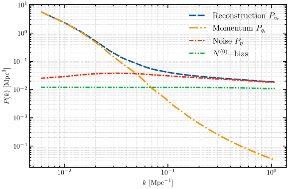
Figure 4: Velocity reconstruction signal and noise power spectra from 100 high resolution Quijote simulations. $P_{{\hat{v}_{r}}}$ and $P_{q_{r}}$ are the power spectra of the noisy velocity reconstruction ${\hat{v}_{r}}$, and the true radial momentum $q_{r}$ (both from simulation). $P_{\eta}$ is the reconstruction noise from simulation, defined as the power spectrum of the noise field $\eta$ defined in Eq. (34). $N_{v_{r}}^{(0)}$ is the kSZ $N^{(0)}$-bias in Eq. (26).

Finally, we come to the main result of this section: comparing the reconstruction noise $P_{\eta}$ in simulation with the kSZ $N^{(0)}$-bias. In Figure 4, we show four power spectra:

• The total power spectrum $P_{{\hat{v}_{r}}}$ of the kSZ velocity reconstruction (including noise), estimated from simulation.

• The power spectrum $P_{q_{r}}$ of the radial momentum, estimated from simulation.

• The reconstruction noise power spectrum $P_{\eta}$, estimated from simulation using the definition of $\eta$ in Eq. (34).

• The kSZ $N^{(0)}$-bias $N_{v_{r}}^{(0)}$, computed using Eq. (26).

Contrary to the prediction from Smith et al. (2018), the reconstruction noise $P_{\eta}$ in simulation exceeds the kSZ $N^{(0)}$-bias by a factor 2–3! This increase in noise can potentially affect $f_{NL}$ constraints, even though the $f_{NL}$ constraints are derived from large scales where the velocity reconstruction is signal-dominated, because sample variance cancellation plays a role in the constraints. We will explore this issue in more detail in §VI and §VII.

As a code check, we also estimated the power spectrum of a “fake” kSZ velocity reconstruction ${\hat{v}_{r}}^{\rm fake}$, constructed by applying the quadratic estimator to a galaxy catalog $\delta_{g}$ and a CMB map $T$ derived from independent $N$-body simulations. The power spectrum of ${\hat{v}_{r}}^{\rm fake}$ is exactly equal to $N_{v_{r}}^{(0)}$, since by construction $N_{v_{r}}^{(0)}$ is the reconstruction noise under the approximation that $\delta_{g}$ and $T$ are independent. In our simulations, we find the expected exact agreement between $P_{\eta}^{\rm fake}$ and $N_{v_{r}}^{(0)}$. This is a strong check on our pipeline, and indicates that the discrepancy between $P_{\eta}$ and $N_{v_{r}}^{(0)}$ is a real effect arising from higher-point correlations in the $N$-body simulation. In §VI, we will explain this discrepancy using the halo model.

V.3 Bandpower covariance

So far, our comparisons between theory and simulation have focused on mean power spectra: either the cross spectrum $P_{{\hat{v}_{r}}q_{r}}$ which determines the bias $b_{v}(k)$, or the noise power spectrum $P_{\eta\eta}$. However, for either forecasts or data analysis, the power spectrum covariance is also important. If the reconstruction noise $\eta$ were a Gaussian field, then its power spectrum covariance would be:

$$\mbox{Cov}(P_{\eta}(b),P_{\eta}(b^{\prime}))=\frac{2}{N_{b}}P_{\eta}(b)^{2}\delta_{bb^{\prime}}$$ (38)

where $b,b^{\prime}$ denote narrow non-overlapping $k$-bins, and $N_{b}$ denotes the number of modes in bin $b$. The standard Fisher matrix forecasting formalism implicitly assumes that the Gaussian bandpower covariance (38) is a good approximation. Our MCMC $f_{NL}$ pipeline in §VII will make slightly stronger assumptions, by assuming that the full probability density function of $\eta$ is well-described by its Gaussian approximation.

As one test of the Gaussian approximation, we estimate the correlation matrix between bandpowers and show the result in Figure 5. We find that non-Gaussian bandpower covariance is small at low $k$, but very significant (correlations of order one) at high $k$. The transition between the two regimes is fairly sharp and occurs at $k\sim 0.03$ Mpc^-1. This suggests that non-Gaussian bandpower covariance is unlikely to be an issue for constraining $f_{NL}$, where statistical weight comes from the very largest scales. (For example, in the $f_{NL}$ analysis in the next section, we will use $k_{\rm max}=0.012$ Mpc^-1.) However, the bandpower covariance in Figure 5 assumes our fiducial survey parameters, and we have not explored parameter dependence systematically.

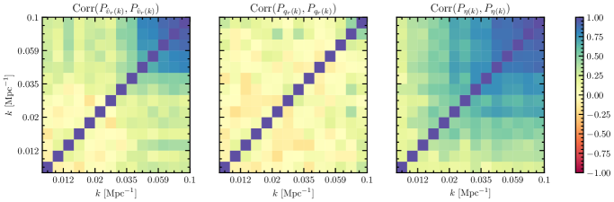
Figure 5: Correlation coefficient between bandpowers $P(k)$ of the velocity reconstruction ${\hat{v}_{r}}({\bf k})$ (left panel), true momentum $q_{r}({\bf k})$ (middle panel), and reconstruction noise $\eta(k)={\hat{v}_{r}}({\bf k})-b_{v}({\bf k})q_{r}({\bf k})$ (right panel). Correlation coefficients were estimated from 100 Quijote simulations.

VI Higher-order biases to kSZ reconstruction noise

In §V.2, we found a discrepancy between the reconstruction noise $P_{\eta}$ in simulation and the kSZ $N^{(0)}$-bias. In this section, we will elaborate on our previous statements that the $N^{(0)}$-bias does not include all terms in the reconstruction noise, derive additional terms which arise in the halo model, and numerically compare the new terms to the simulations.

VI.1 Setup

We will calculate the total power spectrum of the reconstruction $P_{{\hat{v}_{r}}{\hat{v}_{r}}}({\bf k}_{L})$, which will contain all signal and noise terms. First, we set up the calculation using schematic notation which just keeps track of how many terms are present, and how each term factorizes as a product of fields. Since the quadratic estimator has schematic form ${\hat{v}_{r}}\sim(\delta_{g}T)$, its power spectrum has schematic form:

$$P_{{\hat{v}_{r}}{\hat{v}_{r}}}(k_{L})\sim\big{\langle}(\delta_{g}T)(\delta_{g}T)\big{\rangle}\,.$$ (39)

Our calculation will make a series of approximations which we will explain as we go along. First, we make the approximations:

• Approximation 1. We write the CMB as $T=T_{kSZ}+T_{\rm other}$, and make the approximation that the non-kSZ contribution $T_{\rm other}$ is statistically independent of the galaxy catalog. This neglects possible non-Gaussian effects from CMB secondaries, e.g. CMB lensing.

• Approximation 2. The electron radial momentum factorizes as $q_{r}=(1+v_{r})\delta_{e}$ in the kSZ line-of-sight integral (5).

Under these approximations, we can write $P_{{\hat{v}_{r}}{\hat{v}_{r}}}({\bf k}_{L})$ schematically as:

$$P_{{\hat{v}_{r}}{\hat{v}_{r}}}({\bf k}_{L})\sim\big{\langle}\delta_{g}\delta_{g}\big{\rangle}\,\big{\langle}T_{\rm other}T_{\rm other}\big{\rangle}+\big{\langle}(\delta_{g}v_{r}\delta_{e})(\delta_{g}v_{r}\delta_{e})\big{\rangle}$$ (40)

We write the six-point function $\langle(\delta_{g}v_{r}\delta_{e})(\delta_{g}v_{r}\delta_{e})\rangle$ appearing on the RHS as a sum over Wick contractions, plus a non-Gaussian part $\langle(\delta_{g}v_{r}\delta_{e})(\delta_{g}v_{r}\delta_{e})\rangle_{ng}$. There are 15 Wick contractions, but we make the following approximation, which reduces the number to 3:

• Approximation 3. In the Gaussian part of the six-point function $\langle(\delta_{g}v_{r}\delta_{e})(\delta_{g}v_{r}\delta_{e})\rangle$, terms where $v_{r}$ Wick-contracts with either $\delta_{g}$ or $\delta_{e}$ are negligible.

  The rationale for this approximation is as follows. The kSZ velocity reconstruction ${\hat{v}_{r}}({\bf k}_{L})$ is determined by the galaxy and electron fields $\delta_{g}({\bf k}),\delta_{e}({\bf k})$ on “kSZ” scales $k\sim 1$ Mpc^-1. On these scales, radial velocity modes $v_{r}({\bf k})$ are very small, which implies that terms proportional to $P_{gv_{r}}(k)$ and $P_{ev_{r}}(k)$ should also be small.

In this approximation, $P_{{\hat{v}_{r}}}$ has schematic form:

$$P_{{\hat{v}_{r}}}({\bf k}_{L})=\big{\langle}\delta_{g}\delta_{g}\big{\rangle}\,\big{\langle}T_{\rm other}T_{\rm other}\big{\rangle}+\mathop{\vbox{\halign{#\cr\kern 1.72218pt\cr$\hbox{$\hskip 6.11111pt\vrule height=10.97919pt,width=0.29999pt,depth=-0.11153pt\kern-0.29999pt\vrule height=10.97919pt,width=30.03418pt,depth=-10.6792pt\kern-0.29999pt\vrule height=10.97919pt,width=0.29999pt,depth=-0.11153pt$\hss}\hbox{$\hskip 13.80827pt\vrule height=7.31946pt,width=0.29999pt,depth=2.52737pt\kern-0.29999pt\vrule height=7.31946pt,width=30.03418pt,depth=-7.01947pt\kern-0.29999pt\vrule height=7.31946pt,width=0.29999pt,depth=2.52737pt$\hss}\hbox{$\hskip 21.31554pt\vrule height=3.65973pt,width=0.29999pt,depth=-0.11153pt\kern-0.29999pt\vrule height=3.65973pt,width=30.03418pt,depth=-3.35974pt\kern-0.29999pt\vrule height=3.65973pt,width=0.29999pt,depth=-0.11153pt$\hss}$\crcr\kern 1.72218pt\nointerlineskip\cr\hbox{$\displaystyle{(}{\delta}{{}_{g}}{v}{{}_{r}}{\delta}{{}_{e})(}{\delta}{{}_{g}}{v}{{}_{r}}{\delta}_{e})$}\crcr}}}\limits+\mathop{\vbox{\halign{#\cr\kern 1.72218pt\cr$\hbox{$\hskip 6.11111pt\vrule height=7.31946pt,width=0.29999pt,depth=-0.11153pt\kern-0.29999pt\vrule height=7.31946pt,width=15.20442pt,depth=-7.01947pt\kern-0.29999pt\vrule height=7.31946pt,width=0.29999pt,depth=-0.11153pt$\hss}\hbox{$\hskip 13.80827pt\vrule height=3.65973pt,width=0.29999pt,depth=2.52737pt\kern-0.29999pt\vrule height=3.65973pt,width=30.03418pt,depth=-3.35974pt\kern-0.29999pt\vrule height=3.65973pt,width=0.29999pt,depth=2.52737pt$\hss}\hbox{$\hskip 36.1453pt\vrule height=7.31946pt,width=0.29999pt,depth=-0.11153pt\kern-0.29999pt\vrule height=7.31946pt,width=20.33289pt,depth=-7.01947pt\kern-0.29999pt\vrule height=7.31946pt,width=0.29999pt,depth=-0.11153pt$\hss}$\crcr\kern 1.72218pt\nointerlineskip\cr\hbox{$\displaystyle{(}{\delta}{{}_{g}}{v}{{}_{r}}{\delta}{{}_{e})(}{\delta}{{}_{g}}{v}{{}_{r}g}{\delta}_{e})$}\crcr}}}\limits+\mathop{\vbox{\halign{#\cr\kern 1.72218pt\cr$\hbox{$\hskip 6.11111pt\vrule height=10.97919pt,width=0.29999pt,depth=-0.11153pt\kern-0.29999pt\vrule height=10.97919pt,width=45.2386pt,depth=-10.6792pt\kern-0.29999pt\vrule height=10.97919pt,width=0.29999pt,depth=-0.11153pt$\hss}\hbox{$\hskip 13.80827pt\vrule height=7.31946pt,width=0.29999pt,depth=2.52737pt\kern-0.29999pt\vrule height=7.31946pt,width=30.03418pt,depth=-7.01947pt\kern-0.29999pt\vrule height=7.31946pt,width=0.29999pt,depth=2.52737pt$\hss}\hbox{$\hskip 21.31554pt\vrule height=3.65973pt,width=0.29999pt,depth=-0.11153pt\kern-0.29999pt\vrule height=3.65973pt,width=14.82976pt,depth=-3.35974pt\kern-0.29999pt\vrule height=3.65973pt,width=0.29999pt,depth=-0.11153pt$\hss}$\crcr\kern 1.72218pt\nointerlineskip\cr\hbox{$\displaystyle{(}{\delta}{{}_{g}}{v}{{}_{r}}{\delta}{{}_{e})(}{\delta}{{}_{g}}{v}{{}_{r}}{\delta}_{e})$}\crcr}}}\limits+\big{\langle}(\delta_{g}v_{r}\delta_{e})(\delta_{g}v_{r}\delta_{e})\big{\rangle}_{ng}$$ (41)

where the non-Gaussian $n$-point function $\langle\cdot\rangle_{ng}$ denotes the expectation value after subtracting all Wick contractions.

Detailed calculation of each term now shows that the first two terms combine to give the $N^{(0)}$-bias, the third term is the “signal” power spectrum $P_{v_{r}}({\bf k}_{L})$, and the fourth and fifth terms are new reconstruction noise terms $N^{(1)}$ and $N^{(3/2)}$:

$$P_{{\hat{v}_{r}}{\hat{v}_{r}}}({\bf k}_{L})=P_{v_{r}}({\bf k}_{L})+N_{v_{r}}^{(0)}({\bf k}_{L})+N^{(1)}({\bf k}_{L})+N^{(3/2)}({\bf k}_{L})$$ (42)

where the precise (non-schematic) forms of the new bias terms $N^{(1)}$ and $N^{(3/2)}$ are:

$$N^{(1)}({\bf k}_{L}) =N_{v_{r}}^{(0)}({\bf k}_{L})^{2}\,\frac{K_{*}^{4}}{\chi_{*}^{8}}\int\frac{d^{2}{\bf l}}{(2\pi)^{2}}\,\frac{d^{2}{\bf l}^{\prime}}{(2\pi)^{2}}\,\left(\frac{P_{ge}(k_{S})^{2}}{P_{gg}(k_{S})C_{l}^{\rm tot}}\frac{P_{ge}(k^{\prime}_{S})^{2}}{P_{gg}(k^{\prime}_{S})C_{l^{\prime}}^{\rm tot}}P_{v_{r}}({\bf q})\right)_{\begin{subarray}{c}{\bf k}_{S}={\bf k}_{L}+{\bf l}/\chi_{*}\\ {\bf k}^{\prime}_{S}={\bf k}_{L}+{\bf l}^{\prime}/\chi_{*}\\ {\bf q}=-{\bf k}_{L}+({\bf l}+{\bf l}^{\prime})/\chi_{*}\end{subarray}}$$ (43)

$$N^{(3/2)}({\bf k}_{L}) =N_{v_{r}}^{(0)}({\bf k}_{L})^{2}\frac{K_{*}^{4}}{\chi_{*}^{8}}\int\frac{d^{2}{\bf l}}{(2\pi)^{2}}\frac{d^{2}{\bf l}^{\prime}}{(2\pi)^{2}}\frac{d^{3}{\bf q}}{(2\pi)^{3}}\frac{d^{3}{\bf q}^{\prime}}{(2\pi)^{3}}$$

$$\hskip 71.13188pt\times\Bigg{[}\frac{P_{ge}(k_{S})}{P_{gg}(k_{S})C_{l}^{\rm tot}}\frac{P_{ge}(k_{S}^{\prime})}{P_{gg}(k_{S}^{\prime})C_{l^{\prime}}^{\rm tot}}\Big{\langle}\delta_{g}({\bf k}_{S})v_{r}({\bf q})\delta_{e}({\bf p})\delta_{g}^{*}({\bf k}_{S}^{\prime})v_{r}^{*}({\bf q}^{\prime})\delta_{e}^{*}({\bf p}^{\prime})\Big{\rangle}^{\prime}_{ng}\Bigg{]}_{\begin{subarray}{c}{\bf k}_{S}={\bf k}_{L}-{\bf l}/\chi_{*}\\ {\bf k}_{S}^{\prime}={\bf k}_{L}-{\bf l}^{\prime}/\chi*\\ {\bf p}=-{\bf q}+{\bf l}/\chi_{*}\\ {\bf p}^{\prime}=-{\bf q}^{\prime}+{\bf l}^{\prime}/\chi_{*}\end{subarray}}$$ (44)

Here, a primed $N$-point function $\langle\prod_{i=1}^{N}X_{i}({\bf k}_{i})\rangle^{\prime}$ denotes the expectation value without the delta function $(2\pi)^{3}\delta^{3}(\sum{\bf k}_{i})$.

We have chosen to call the new terms the kSZ $N^{(1)}$-bias and $N^{(3/2)}$-bias, to emphasize an analogy with CMB lensing. The $N^{(0)}$ and $N^{(1)}$ biases represent the total KSZ reconstruction noise if all LSS fields are Gaussian. The $N^{(1)}$-bias is a Wick contraction which is more difficult to compute, since the integrals cannot be factored into a sequence of convolutions. The $N^{(3/2)}$-bias represents additional noise bias arising from non-Gaussianity of the LSS fields ($\delta_{g}$ and $\delta_{e}$). All of these statements are also true for the CMB lensing $N^{(1)}$-bias Kesden et al. (2003) and $N^{(3/2)}$-bias Böhm et al. (2016). However, the analogy is not perfect: in the CMB lensing case, there is a systematic expansion in powers of the lensing potential $\phi$, and there is no analogous expansion in the kSZ case. On a related note, when we evaluate the kSZ biases numerically, we will find that the $N^{(1)}$-bias is much smaller than $N^{(0)}$, whereas the $N^{(3/2)}$-bias is comparable to $N^{(0)}$.

VI.2 KSZ $N^{(1)}$-bias

In the limit $k_{L}\ll k_{S}$, the $N^{(1)}$-bias in Eq. (43) can be simplified a lot. We make the following approximations inside the integral:

$$N_{v_{r}}^{(0)}({\bf k}_{L})\approx N_{v_{r}}^{(0)}(0)\hskip 28.45274pt{\bf k}_{S}={\bf k}_{L}+{\bf l}/\chi_{*}\approx{\bf l}/\chi_{*}\hskip 28.45274pt{\bf k}_{S}^{\prime}=-{\bf q}+{\bf l}/\chi_{*}\approx{\bf l}/\chi_{*}$$ (45)

where the third approximation is valid since the integrand contains the factor $P_{v_{r}}({\bf q})$, which peaks for $q\ll k_{S}$. Making these approximations in Eq. (43), and changing variables from ${\bf l}^{\prime}$ to ${\bf l}^{\prime\prime}=({\bf l}+{\bf l}^{\prime})$, the integral factorizes as:

$$N^{(1)}({\bf k}_{L})\approx N_{v_{r}}^{(0)}(0)^{2}\,\frac{K_{*}^{4}}{\chi_{*}^{8}}\left(\int\frac{d^{2}{\bf l}}{(2\pi)^{2}}\,\frac{P_{ge}(k_{S})^{4}}{P_{gg}(k_{S})^{2}(C_{l}^{\rm tot})^{2}}\right)_{k_{S}=l/\chi_{*}}\left(\int\frac{d^{2}{\bf l}^{\prime\prime}}{(2\pi)^{2}}\,P_{v_{r}}({\bf q})\right)_{{\bf q}=-{\bf k}_{L}+{\bf l}^{\prime\prime}/\chi_{*}}$$ (46)

We simplify the second factor as:

$$\left(\int\frac{d^{2}{\bf l}^{\prime\prime}}{(2\pi)^{2}}\,P_{v_{r}}({\bf q})\right)_{{\bf q}=-{\bf k}_{L}+{\bf l}^{\prime\prime}/\chi_{*}} =k_{Lr}^{2}\int\frac{d^{2}{\bf l}^{\prime\prime}}{(2\pi)^{2}}\,\left(\frac{P_{v}(q)}{q^{2}}\right)_{{\bf q}=-{\bf k}_{L}+{\bf l}^{\prime\prime}/\chi_{*}} P_{v_{r}}(q)=(k_{Lr}/q)^{2}P_{v}(q)$$ since

$$=\frac{k_{Lr}^{2}\chi_{*}^{2}}{2\pi}\int_{|k_{Lr}|}^{\infty}dq\frac{P_{v}(q)}{q}$$ by change of variables (47)

To make the first factor more intuitive, we define the dimensionless quantity:

$$W(l)=N_{v_{r}}^{(0)}(0)\frac{K_{*}^{2}}{\chi_{*}^{4}}\left(\frac{P_{ge}(k_{S})^{2}}{P_{gg}(k_{S})C_{l}^{\rm tot}}\right)_{{\bf k}_{S}={\bf l}/\chi_{*}}$$ (48)

which satisfies (using Eq. (26)):

$$\int\frac{d^{2}{\bf l}}{(2\pi)^{2}}\,W(l)=1\,.$$ (49)

Plugging into Eq. (46) we get:

$$N^{(1)}({\bf k}_{L})\approx\frac{k_{Lr}^{2}\chi_{*}^{2}}{2\pi}\left(\int\frac{d^{2}{\bf l}}{(2\pi)^{2}}\,W(l)^{2}\right)\left(\int_{|k_{Lr}|}^{\infty}dq\frac{P_{v}(q)}{q}\right)\hskip 42.67912pt(k_{L}\ll k_{S})$$ (50)

Note that for $k_{L}\ll k_{S}$, the $N^{(1)}$-bias only depends on $|k_{Lr}|=|\mu|k_{L}$. In the limit $k_{Lr}\ll k_{eq}$, where $k_{eq}\sim 0.02$ Mpc^-1 is the matter-radiation equality scale, $N^{(1)}(k_{Lr})$ is proportional to $|k_{Lr}|$. (In contrast to the $N^{(0)}$-bias, which is constant on large scales.)

It will also be useful to have an expression for the $N^{(1)}$-bias after angle-averaging ${\bf k}_{L}$ (e.g. in Figure 6 below). We omit the details of the calculation and quote the final result:

$$N^{(1)}(k_{L})_{\rm avg}\approx\frac{\chi_{*}^{2}}{6\pi}\left(\int\frac{d^{2}{\bf l}}{(2\pi)^{2}}\,W(l)^{2}\right)\left(\frac{1}{k_{L}}\int_{0}^{k_{L}}dq\,q^{2}P_{v}(q)+k_{L}^{2}\int_{k_{L}}^{\infty}dq\,\frac{P_{v}(q)}{q}\right)$$ (51)

where “avg” means “angle-averaged over ${\bf k}_{L}$”, and $k_{L}\ll k_{S}$ has been assumed.

VI.3 KSZ $N^{(3/2)}$-bias and halo model evaluation

In the limit $k_{L}\ll k_{S}$, the $N^{(3/2)}$-bias in Eq. (44) also simplifies. We start by using the halo model to compute the non-Gaussian six-point function:

$$\big{\langle}\delta_{g}({\bf k}_{1})\delta_{e}({\bf k}_{2})\delta_{g}({\bf k}_{3})\delta_{e}({\bf k}_{4})v_{r}({\bf k}_{5})v_{r}({\bf k}_{6})\big{\rangle}^{\prime}_{ng}$$ (52)

which appears in $N^{(3/2)}$.

We briefly summarize the ingredients of the halo model; for a systematic review see Cooray and Sheth (2002). Let $n(M)$ be the halo mass function, or number of halos per unit volume per unit halo mass. Let $b(M)$ be the large-scale bias of a halo of mass $M$. Let $n_{h}=\int_{M_{\rm min}}^{\infty}dM\,n(M)$ be the mean halo number density, and let $\rho_{m}$ be the mean matter density. Here, $M_{\rm min}$ is the minimum halo mass for our catalog (corresponding to 40 particles). Let $u_{M}(k)$ be the Fourier-transformed mass profile of a halo of mass $M$, normalized so that $u_{M}(0)=1$.

It will be convenient to define:

$$\alpha_{n}(k_{1},\cdots,k_{n}) =\frac{1}{n_{h}}\int_{M_{\rm min}}^{\infty}dM\,n(M)\,\prod_{i=1}^{n}\frac{Mu_{M}(k_{i})}{\rho_{m}}$$ (53)

$$\beta_{n}(k_{1},\cdots,k_{n}) =\frac{1}{n_{h}}\int_{M_{\rm min}}^{\infty}dM\,n(M)b(M)\,\prod_{i=1}^{n}\frac{Mu_{M}(k_{i})}{\rho_{m}}$$ (54)

$$\beta_{n}^{\prime}(k_{1},\cdots,k_{n}) =\frac{1}{n_{h}}\int_{0}^{\infty}dM\,n(M)b(M)\,\prod_{i=1}^{n}\frac{Mu_{M}(k_{i})}{\rho_{m}}$$ (55)

Note that for $n=0$, we have $\alpha_{0}=1$ and $\beta_{0}=b$, where $b=n_{h}^{-1}\int_{M_{\rm min}}^{\infty}dM\,n(M)b(M)$ is the halo bias.

Under the assumptions of the halo model, the connected six-point function in Eq. (52) can be calculated exactly. In Appendix A, we present the details of the calculation, and diagrammatic rules for calculating $n$-point functions in the halo model, which may be of more general interest. In the next few paragraphs (Eqs. (56)–(66)), we summarize the result of the calculation.

We assume that the radial velocity modes $v_{r}({\bf k}_{5}),v_{r}({\bf k}_{6})$ in the six-point function (52) are evaluated on linear scales ${\bf k}_{5},{\bf k}_{6}$. Then the six-point function factorizes into lower-order correlation functions (i.e. there are no fully connected contributions). More precisely, the six-point function (52) is given by:

$$\big{\langle}\delta_{g}({\bf k}_{1})\delta_{e}({\bf k}_{2})\delta_{g}({\bf k}_{3})\delta_{e}({\bf k}_{4})v_{r}({\bf k}_{5})v_{r}({\bf k}_{6})\big{\rangle}_{ng}$$

$$\hskip 28.45274pt=\Big{[}\big{(}Q^{ge}_{{\bf k}_{1}{\bf k}_{2}{\bf k}_{5}}Q^{ge}_{{\bf k}_{3}{\bf k}_{4}{\bf k}_{6}}+Q^{gg}_{{\bf k}_{1}{\bf k}_{3}{\bf k}_{5}}Q^{ee}_{{\bf k}_{2}{\bf k}_{4}{\bf k}_{6}}+Q^{ge}_{{\bf k}_{1}{\bf k}_{4}{\bf k}_{5}}Q^{ge}_{{\bf k}_{2}{\bf k}_{3}{\bf k}_{6}}\big{)}+\big{(}{\bf k}_{5}\leftrightarrow{\bf k}_{6}\big{)}\Big{]}$$

$$\hskip 42.67912pt+\Big{[}\big{(}P^{\delta_{g}v_{r}}_{{\bf k}_{1}{\bf k}_{5}}R^{ege}_{{\bf k}_{2}{\bf k}_{3}{\bf k}_{4}{\bf k}_{6}}+P^{\delta_{e}v_{r}}_{{\bf k}_{2}{\bf k}_{5}}R^{gge}_{{\bf k}_{1}{\bf k}_{3}{\bf k}_{4}{\bf k}_{6}}+P^{\delta_{e}v_{r}}_{{\bf k}_{3}{\bf k}_{5}}R^{gee}_{{\bf k}_{1}{\bf k}_{2}{\bf k}_{4}{\bf k}_{6}}+P^{\delta_{e}v_{r}}_{{\bf k}_{4}{\bf k}_{5}}R^{geg}_{{\bf k}_{1}{\bf k}_{2}{\bf k}_{3}{\bf k}_{6}}\big{)}+\big{(}{\bf k}_{5}\leftrightarrow{\bf k}_{6}\big{)}\Big{]}$$

$$\hskip 42.67912pt+\Big{[}S_{{\bf k}_{1}{\bf k}_{2}{\bf k}_{3}{\bf k}_{4}}P^{v_{r}v_{r}}_{{\bf k}_{5}{\bf k}_{6}}\Big{]}$$ (56)

where we have introduced the following notation for some 2-, 3-, and 4-point functions:

$$P^{XY}_{{\bf k}_{1}{\bf k}_{2}} =\big{\langle}X({\bf k}_{1})Y({\bf k}_{2})\big{\rangle} (X,Y\in\{\delta_{g},\delta_{e},v_{r}\})$$ (57)

$$Q^{XY}_{{\bf k}_{1}{\bf k}_{2}{\bf k}_{3}} =\big{\langle}\delta_{X}({\bf k}_{1})\delta_{Y}({\bf k}_{2})v_{r}({\bf k}_{3})\big{\rangle} (X,Y\in\{g,e\})$$ (58)

$$R^{XYZ}_{{\bf k}_{1}{\bf k}_{2}{\bf k}_{3}{\bf k}_{4}} =\big{\langle}\delta_{X}({\bf k}_{1})\delta_{Y}({\bf k}_{2})\delta_{Z}({\bf k}_{3})v_{r}({\bf k}_{4})\big{\rangle}_{ng} (X,Y,Z\in\{g,e\})$$ (59)

$$S_{{\bf k}_{1}{\bf k}_{2}{\bf k}_{3}{\bf k}_{4}} =\big{\langle}\delta_{g}({\bf k}_{1})\delta_{e}({\bf k}_{2})\delta_{g}({\bf k}_{3})\delta_{e}({\bf k}_{4})\big{\rangle}_{ng}$$ (60)

The quantities $Q,R,S$ on the RHS of Eq. (56) are given explicitly by:

$$Q^{ge}_{{\bf k}_{1}{\bf k}_{2}{\bf k}_{3}} =\beta_{1}(k_{2})\left(\frac{ik_{3r}}{k_{3}}\right)P_{mv}(k_{3})\,(2\pi)^{3}\delta^{3}\left(\mathop{\textstyle\sum}\limits{\bf k}_{i}\right)$$ (61)

$$Q^{gg}_{{\bf k}_{1}{\bf k}_{2}{\bf k}_{3}} =\frac{b}{n_{h}}\left(\frac{ik_{3r}}{k_{3}}\right)P_{mv}(k_{3})\,(2\pi)^{3}\delta^{3}\left(\mathop{\textstyle\sum}\limits{\bf k}_{i}\right)$$ (62)

$$Q^{ee}_{{\bf k}_{1}{\bf k}_{2}{\bf k}_{3}} =n_{h}\beta_{2}^{\prime}(k_{1},k_{2})\left(\frac{ik_{3r}}{k_{3}}\right)P_{mv}(k_{3})\,(2\pi)^{3}\delta^{3}\left(\mathop{\textstyle\sum}\limits{\bf k}_{i}\right)$$ (63)

$$R^{gge}_{{\bf k}_{1}{\bf k}_{2}{\bf k}_{3}{\bf k}_{4}} =\frac{\beta_{1}(k_{3})}{n_{h}}\left(\frac{ik_{4r}}{k_{4}}\right)P_{mv}(k_{4})\,(2\pi)^{3}\delta^{3}\left(\mathop{\textstyle\sum}\limits{\bf k}_{i}\right)$$ (64)

$$R^{gee}_{{\bf k}_{1}{\bf k}_{2}{\bf k}_{3}{\bf k}_{4}} =\beta_{2}(k_{2},k_{3})\left(\frac{ik_{4r}}{k_{4}}\right)P_{mv}(k_{4})\,(2\pi)^{3}\delta^{3}\left(\mathop{\textstyle\sum}\limits{\bf k}_{i}\right)$$ (65)

$$S_{{\bf k}_{1}{\bf k}_{2}{\bf k}_{3}{\bf k}_{4}} =\Bigg{[}\frac{\alpha_{2}(k_{2},k_{4})}{n_{h}}+\beta_{1}(k_{2})\beta_{1}(k_{4})P_{\rm lin}({\bf k}_{1}+{\bf k}_{2})+b\beta_{2}^{\prime}(k_{2},k_{4})P_{\rm lin}({\bf k}_{1}+{\bf k}_{3})$$

$$\hskip 21.33955pt+\beta_{1}(k_{2})\beta_{1}(k_{4})P_{\rm lin}({\bf k}_{1}+{\bf k}_{4})+b\beta_{2}(k_{2},k_{4})P_{\rm lin}(k_{1})+\beta_{1}^{\prime}(k_{2})\beta_{1}(k_{4})P_{\rm lin}(k_{2})$$

$$\hskip 21.33955pt+b\beta_{2}(k_{2},k_{4})P_{\rm lin}(k_{3})+\beta_{1}(k_{2})\beta_{1}^{\prime}(k_{4})P_{\rm lin}(k_{4})\bigg{]}(2\pi)^{3}\delta^{3}(\mathop{\textstyle\sum}\limits{\bf k}_{i})$$ (66)

where $P_{mv}(k)=(faH/k)P_{\rm lin}(k)$ is the linear matter-velocity power spectrum.

Taken together, Eqs. (56)–(66)) are a complete calculation of the six-point function (52) in the halo model, in a rather daunting form with 22 terms! However, we will now argue that most of these terms are negligible, when we compute the $N^{(3/2)}$-bias by plugging the six-point function into the integral (44).

In the integral (44), the six-point function is evaluated at the following configuration of wavenumbers ${\bf k}_{1},\cdots,{\bf k}_{6}$:

$${\bf k}_{1}={\bf k}_{L}-\frac{{\bf l}}{\chi_{*}}\hskip 22.76228pt{\bf k}_{2}=-{\bf q}+\frac{{\bf l}}{\chi_{*}}\hskip 22.76228pt{\bf k}_{3}=-{\bf k}_{L}+\frac{{\bf l}^{\prime}}{\chi_{*}}\hskip 22.76228pt{\bf k}_{4}={\bf q}^{\prime}-\frac{{\bf l}^{\prime}}{\chi_{*}}\hskip 22.76228pt{\bf k}_{5}={\bf q}\hskip 22.76228pt{\bf k}_{6}=-{\bf q}^{\prime}$$ (67)

To understand which terms are negligible, we classify wavenumbers as either “small-scale” (meaning a typical kSZ scale $\sim$1 Mpc^-1), or “large-scale” (meaning $\ll 1$ Mpc^-1). In the integral (44), we formally integrate over all wavenumbers $({\bf l},{\bf l}^{\prime},{\bf q},{\bf q}^{\prime})$, but we will assume that $q,q^{\prime}$ are large-scale , and $(l/\chi_{*}),(l^{\prime}/\chi_{*})$ are small-scale, since these wavenumber configurations dominate the integral. We will also assume that $k_{L}$ is large-scale, since we are interested in the $N^{(3/2)}$-bias in the limit $k_{L}\rightarrow 0$.

Now we can state our criteria for deciding which terms in the six-point function are negligible:

• Approximation 4. In the six-point function (52), terms where $P_{\rm lin}$ is evaluated at a small-scale wavenumber give negligible contributions to $N^{(3/2)}$.

  Rationale: On a small scale $k$, clustering is small compared to halo shot noise, so terms in the reconstruction noise proportional to $P_{\rm lin}(k)$ should be subdominant to other contributions.

• Approximation 5. Each term in the “primed” six-point function (52) contains a single delta function $\delta^{3}(\cdots)$. If the delta function argument is a small-scale wavenumber (in the sense defined above), then we assume that the six-point term under consideration gives a negligible contribution to $N^{(3/2)}$. For example, the term $(Q^{gg}_{{\bf k}_{1}{\bf k}_{3}{\bf k}_{6}}Q^{ee}_{{\bf k}_{2}{\bf k}_{4}{\bf k}_{5}})$ containing the delta function $\delta^{3}({\bf q}+({\bf l}-{\bf l}^{\prime})/\chi_{*})$ is negligible, whereas the term $(Q^{gg}_{{\bf k}_{1}{\bf k}_{2}{\bf k}_{6}}Q^{ee}_{{\bf k}_{2}{\bf k}_{3}{\bf k}_{5}})$ containing the delta function $\delta^{3}({\bf k}_{L}-{\bf q}-{\bf q}^{\prime})$ is non-negligible.

  Rationale: In Eq. (44), the $N^{(3/2)}$-bias is computed by by integrating over small-scale wavenumbers $({\bf l}/\chi_{*}),({\bf l}/\chi_{*})$ and large-scale wavenumbers ${\bf q},{\bf q}^{\prime}$. If the six-point function contains a term such as $\delta^{3}({\bf q}+({\bf l}-{\bf l}^{\prime})/\chi_{*})$, this imposes a constraint that $({\bf l}-{\bf l}^{\prime})/\chi_{*}$ be a large-scale wavenumber, which is only satisfied in a small part of the $({\bf l},{\bf l}^{\prime})$-plane. Therefore we expect a small contribution to $N^{(3/2)}$.

Most of the six-point terms in Eq. (56) are eliminated using these criteria. On the first line of (56), all of the $QQ$-terms are eliminated using Approximation 5, except $(Q^{ge}_{{\bf k}_{1}{\bf k}_{2}{\bf k}_{6}}Q^{ge}_{{\bf k}_{3}{\bf k}_{4}{\bf k}_{5}})$ which is non-negligible, and $(Q^{ge}_{{\bf k}_{1}{\bf k}_{2}{\bf k}_{5}}Q^{ge}_{{\bf k}_{3}{\bf k}_{4}{\bf k}_{6}})$ which is a special case: it contains the delta function $\delta^{3}({\bf k}_{L})$, and we neglect it since we are interested in the $N^{(3/2)}$-bias for nonzero $k_{L}$. All eight $PR$-terms on the second line of Eq. (56) are eliminated using Approximation 5. Finally, the last six $S$-terms (out of eight total $S$-terms) in Eq. (66) are eliminated using Approximation 4. For example, the third term in (66) contains $P_{\rm lin}({\bf k}_{1}+{\bf k}_{3})=P_{\rm lin}(({\bf l}-{\bf l}^{\prime})/\chi_{*})$, and $({\bf l}-{\bf l}^{\prime})/\chi_{*}$ is small-scale (except in a small part of the $({\bf l},{\bf l}^{\prime})$-plane).

Summarizing this section so far, we have argued only three terms (out of 22) in the six-point function (56) contribute significantly to the $N^{(3/2)}$ bias:

$$\big{\langle}\delta_{g}({\bf k}_{1})\delta_{e}({\bf k}_{2})\delta_{g}({\bf k}_{3})\delta_{e}({\bf k}_{4})v_{r}({\bf k}_{5})v_{r}({\bf k}_{6})\big{\rangle}^{\prime}_{ng}$$

$$\hskip 42.67912pt\approx-\beta_{1}(k_{2})\beta_{1}(k_{4})\left(\frac{k_{5r}k_{6r}}{k_{5}k_{6}}\right)P_{mv}(k_{5})P_{mv}(k_{6})(2\pi)^{3}\delta^{3}({\bf k}_{1}+{\bf k}_{2}+{\bf k}_{6})$$

$$\hskip 56.9055pt+\left(\frac{\alpha_{2}(k_{2},k_{4})}{n_{h}}+\beta_{1}(k_{2})\beta_{1}(k_{4})P_{\rm lin}({\bf k}_{1}+{\bf k}_{2})\right)P_{v_{r}}({\bf k}_{5})(2\pi)^{3}\delta^{3}({\bf k}_{5}+{\bf k}_{6})$$ (68)

Using this expression, we now proceed to compute the $N^{(3/2)}$-bias, by plugging the six-point function (68) into our general expression (44) for the $N^{(3/2)}$-bias, obtaining:

$$N^{(3/2)}({\bf k}_{L}) =N_{v_{r}}^{(0)}({\bf k}_{L})^{2}\frac{K_{*}^{4}}{\chi_{*}^{8}}\int\frac{d^{2}{\bf l}}{(2\pi)^{2}}\frac{d^{2}{\bf l}^{\prime}}{(2\pi)^{2}}\frac{d^{3}{\bf q}}{(2\pi)^{3}}\,$$

$$\hskip 28.45274pt\times\Bigg{[}\frac{P_{ge}(k_{S})}{P_{gg}(k_{S})C_{l}^{\rm tot}}\frac{P_{ge}(k_{S}^{\prime})}{P_{gg}(k_{S}^{\prime})C_{l^{\prime}}^{\rm tot}}\beta_{1}(p)\beta_{1}(p^{\prime})\left(\frac{q_{r}q^{\prime}_{r}}{qq^{\prime}}\right)P_{mv}(q)P_{mv}(q^{\prime})\Bigg{]}_{\begin{subarray}{c}{\bf k}_{S}={\bf k}_{L}-{\bf l}/\chi_{*}\\ {\bf k}_{S}^{\prime}={\bf k}_{L}-{\bf l}^{\prime}/\chi*\\ {\bf q}^{\prime}={\bf k}_{L}-{\bf q}\\ {\bf p}=-{\bf q}+{\bf l}/\chi_{*}\\ {\bf p}^{\prime}=-{\bf q}^{\prime}+{\bf l}^{\prime}/\chi_{*}\end{subarray}}$$

$$+N_{v_{r}}^{(0)}({\bf k}_{L})^{2}\frac{K_{*}^{4}}{\chi_{*}^{8}}\int\frac{d^{2}{\bf l}}{(2\pi)^{2}}\frac{d^{2}{\bf l}^{\prime}}{(2\pi)^{2}}\frac{d^{3}{\bf q}}{(2\pi)^{3}}\,$$

$$\hskip 28.45274pt\times\Bigg{[}\frac{P_{ge}(k_{S})}{P_{gg}(k_{S})C_{l}^{\rm tot}}\frac{P_{ge}(k_{S}^{\prime})}{P_{gg}(k_{S}^{\prime})C_{l^{\prime}}^{\rm tot}}\left(\frac{\alpha_{2}(p,p^{\prime})}{n_{h}}+\beta_{1}(p)\beta_{1}(p^{\prime})P_{\rm lin}({\bf k}_{L}-{\bf q})\right)P_{v_{r}}({\bf q})\Bigg{]}_{\begin{subarray}{c}{\bf k}_{S}={\bf k}_{L}-{\bf l}/\chi_{*}\\ {\bf k}_{S}^{\prime}={\bf k}_{L}-{\bf l}^{\prime}/\chi*\\ {\bf p}=-{\bf q}+{\bf l}/\chi_{*}\\ {\bf p}^{\prime}=-{\bf q}+{\bf l}^{\prime}/\chi_{*}\end{subarray}}$$ (69)

We make the following approximations inside the integrals, which are valid for $k_{L}\ll k_{S}$:

$$N_{v_{r}}({\bf k}_{L})\approx N_{v_{r}}(0)\hskip 42.67912ptk_{S}\approx p\approx l/\chi_{*}\hskip 42.67912ptk_{S}^{\prime}\approx p^{\prime}\approx l^{\prime}/\chi_{*}$$ (70)

as in the $N^{(1)}$ case (see discussion near Eq. (45)). We also write $P_{\rm lin}(q^{\prime})P_{v_{r}}(q)=P_{mv}(q^{\prime})P_{mv}(q)\,q_{r}^{2}/(qq^{\prime})$, to combine the two terms in (69) into a single term:

$$N^{(3/2)}({\bf k}_{L}) \approx N_{v_{r}}^{(0)}(0)^{2}\frac{K_{*}^{4}}{\chi_{*}^{8}}\int\frac{d^{2}{\bf l}}{(2\pi)^{2}}\frac{d^{2}{\bf l}^{\prime}}{(2\pi)^{2}}\frac{d^{3}{\bf q}}{(2\pi)^{3}}\,$$

$$\hskip 14.22636pt\times\Bigg{[}\frac{P_{ge}(k_{S})}{P_{gg}(k_{S})C_{l}^{\rm tot}}\frac{P_{ge}(k_{S}^{\prime})}{P_{gg}(k_{S}^{\prime})C_{l^{\prime}}^{\rm tot}}\left(\frac{\alpha_{2}(k_{S},k_{S}^{\prime})}{n_{h}}P_{v_{r}}(q)+\beta_{1}(k_{S})\beta_{1}(k_{S}^{\prime})\left(\frac{q_{r}^{2}+q_{r}q^{\prime}_{r}}{qq^{\prime}}\right)P_{mv}(q)P_{mv}(q^{\prime})\right)\Bigg{]}_{\begin{subarray}{c}k_{S}=l/\chi_{*}\\ k_{S}^{\prime}=l^{\prime}/\chi*\\ {\bf q}^{\prime}={\bf k}_{L}-{\bf q}\\ \end{subarray}}$$ (71)

We symmetrize the integrand by replacing $(q_{r}^{2}+q_{r}q_{r}^{\prime})\rightarrow(q_{r}+q_{r}^{\prime})^{2}/2=k_{Lr}^{2}/2$, and use the definition of $W(l)$ in Eq. (48), obtaining:

$$N^{(3/2)}({\bf k}_{L}) \approx\int\frac{d^{2}{\bf l}}{(2\pi)^{2}}\frac{d^{2}{\bf l}^{\prime}}{(2\pi)^{2}}\frac{d^{3}{\bf q}}{(2\pi)^{3}}W(l)W(l^{\prime})$$

$$\hskip 28.45274pt\times\Bigg{[}\frac{1}{P_{ge}(k_{S})P_{ge}(k_{S}^{\prime})}\left(\frac{\alpha_{2}(k_{S},k_{S}^{\prime})}{n_{h}}P_{v_{r}}(q)+\beta_{1}(k_{S})\beta_{1}(k_{S}^{\prime})\left(\frac{k_{Lr}^{2}}{2qq^{\prime}}\right)P_{mv}(q)P_{mv}(q^{\prime})\right)\Bigg{]}_{\begin{subarray}{c}k_{S}=l/\chi_{*}\\ k_{S}^{\prime}=l^{\prime}/\chi*\\ {\bf q}^{\prime}={\bf k}_{L}-{\bf q}\\ \end{subarray}}$$

So far, our approximations should be very accurate in the limit $k_{L}\ll k_{S}$. To simplify further, we make two more approximations that are not as precise, but should suffice for an initial estimate of the size of $N^{(3/2)}$. First, we assume that on kSZ scales, the galaxy-electron power spectrum is dominated by its 1-halo term:

$$P_{ge}(k_{S})\sim P_{ge}^{1h}(k_{S})=\frac{1}{\rho_{m}n_{h}}\int dM\,n(M)Mu_{M}(k_{S})$$ (73)

We then write some of the intermediate quantities which appear in the integral (LABEL:eq:n32_long2) as follows:

$$\frac{\alpha_{2}(k_{S},k_{S}^{\prime})}{P_{ge}(k_{S})P_{ge}(k_{S}^{\prime})} \sim\frac{\big{\langle}M^{2}u_{M}(k_{S})u_{M}(k_{S}^{\prime})\big{\rangle}_{M}}{\big{\langle}Mu_{M}(k_{S})\big{\rangle}_{M}\,\big{\langle}M^{\prime}u_{M^{\prime}}(k_{S}^{\prime})\big{\rangle}_{M^{\prime}}}$$ (74)

$$\frac{\beta_{1}(k_{S})}{P_{ge}(k_{S})} \sim\frac{\big{\langle}Mb(M)u_{M}(k_{S})\big{\rangle}_{M}}{\big{\langle}Mu_{M}(k_{S})\big{\rangle}_{M}}$$ (75)

where we have introduced the following notation, to denote an average over halos in the catalog:

$$\big{\langle}\cdots\big{\rangle}_{M}=\frac{1}{n_{h}}\int_{M_{\rm min}}^{\infty}n(M)\,(\cdots)$$ (76)

Our second approximation is that the factors $u_{M}(k_{S})$ approximately cancel on the RHS of (74), (75), since they appear in both the numerator and denominator. Then the right-hand sides of Eqs. (74), (75) simplify as:

$$\frac{\alpha_{2}(k_{S},k_{S}^{\prime})}{P_{ge}(k_{S})P_{ge}(k_{S}^{\prime})}\sim A\hskip 42.67912pt\frac{\beta_{1}(k_{S})}{P_{ge}(k_{S})}\sim B$$ (77)

where the dimensionless constants $A,B$ are defined by:

$$A=\frac{\langle M^{2}\rangle_{M}}{\langle M\rangle_{M}^{2}}\hskip 42.67912ptB=\frac{\langle Mb(M)\rangle_{M}}{\langle M\rangle_{M}}$$ (78)

Making the approximations (77) in Eq. (LABEL:eq:n32_long2), the $N^{(3/2)}$-bias simplifies significantly:

$$N^{(3/2)}({\bf k}_{L}) \sim\int\frac{d^{2}{\bf l}}{(2\pi)^{2}}\frac{d^{2}{\bf l}^{\prime}}{(2\pi)^{2}}\frac{d^{3}{\bf q}}{(2\pi)^{3}}\,W(l)W(l^{\prime})\left[\frac{A}{n_{h}}P_{v_{r}}(q)+\frac{B^{2}k_{Lr}^{2}}{2qq^{\prime}}P_{mv}(q)P_{mv}(q^{\prime})\right]_{{\bf q}^{\prime}={\bf k}_{L}-{\bf q}}$$

$$=\frac{A}{n_{h}}\langle v_{r}^{2}\rangle+\frac{B^{2}k_{Lr}^{2}}{2}\int\frac{d^{3}{\bf q}}{(2\pi)^{3}}\,\left[\frac{P_{mv}(q)P_{mv}(q^{\prime})}{qq^{\prime}}\right]_{{\bf q}^{\prime}={\bf k}_{L}-{\bf q}}$$ (79)

where in the second line, we have used $\int d^{2}{\bf l}/(2\pi)^{2}\,W(l)=1$, and $\langle v_{r}^{2}\rangle$ denotes the variance of the radial velocity field:

$$\langle v_{r}^{2}\rangle\equiv\int\frac{d^{3}{\bf k}}{(2\pi)^{3}}P_{v_{r}}(k)=\int\frac{k^{2}\,dk}{6\pi^{2}}P_{v}(k)$$ (80)

Finally, we note that in the 3-d integral (79), one angular integral can be done analytically, reducing to a 2-d integral. We omit the details and quote the final result:

$$N^{(3/2)}({\bf k}_{L})\sim\frac{A}{n_{h}}\langle v_{r}^{2}\rangle+\frac{B^{2}k_{Lr}^{2}}{8\pi^{2}k_{L}}\int_{0}^{\infty}dq\int_{|k_{L}-q|}^{k_{L}+q}dq^{\prime}\,P_{mv}(q)P_{mv}(q^{\prime})$$ (81)

To angle-average over ${\bf k}_{L}$ (as we will do in Figure 6 shortly), we replace $k_{Lr}^{2}\rightarrow k_{L}^{2}/3$ in the second term. The $A$-term in Eq. (81) is constant in $k_{L}$, and the $B$-term goes to zero at both low and high $k_{L}$, with a peak at $k_{L}\sim 0.03$ Mpc^-1.

VI.4 Numerical evaluation and discussion

In the last few sections, we identified several new contributions to the kSZ reconstruction noise, going beyond the $N^{(0)}$-bias from Smith and Ferraro (2017). Can these new contributions explain the excess noise in our simulations, shown previously in Figure 4?

In Figure 6, we numerically evaluate the $N^{(0)}$, $N^{(1)}$, and $N^{(3/2)}$ biases as follows. All power spectra are angle-averaged over ${\bf k}$. We compute the $N^{(0)}$-bias using Eqs. (30), (31), but to maximize consistency with our simulations, we replace integrals (either $\int d^{3}{\bf x}$, $\int d^{3}{\bf k}$, or $\int d^{2}{\bf l}$) by sums over the discrete set of pixels (or Fourier modes) used in our simulation pipeline.

We compute the angle-averaged $N^{(1)}$-bias using Eq. (51), and the $N^{(3/2)}$-bias using Eq. (81). Note that (51) and (81) are approximations which are accurate for $k\rightarrow 0$. To evaluate (81), we need numerical values for the constants $A,B$ defined in Eq. (78). We get $A=2.3$ using the measured halo mass function from our $N$-body simulations. We approximate $B\sim b_{g}$, where $b_{g}=3.24$ is the halo bias of our simulations. (This is an approximation since $b_{g}$ is calculated weighting all halos equally, whereas $B$ is the mass-weighted halo bias.)

Our first result in Figure 6 is that the $N^{(1)}$-bias is negligible. As a check on our $N^{(1)}$ calculation, we compared to Gaussian Monte Carlo simulations which are designed to isolate the $N^{(1)}$-bias, and find good agreement. In more detail, each Gaussian simulation consists of 3-d Gaussian fields $v_{r},\delta_{g},\delta_{e}$ with the same auto and cross power spectra as the Quijote simulations. For each triple $(i,j,k)$ of Gaussian simulations, let ${\hat{v}_{r}}^{ijk}$ denote the kSZ velocity reconstruction using fields $v_{r}^{i}$, $\delta_{g}^{j}$, $\delta_{e}^{k}$ from simulations $i,j,k$. Then the cross power spectrum between ${\hat{v}_{r}}^{ijk}$ and ${\hat{v}_{r}}^{ikj}$ is equal to $N^{(1)}$, with no $N^{(0)}$ or $N^{(3/2)}$ contribution, since $N^{(1)}$ is the only surviving contraction in Eq. (41).

Our main result in Figure 6 is that the $N^{(3/2)}$-bias agrees well with the excess noise seen in simulations! (Surprisingly, the agreement holds to high $k$, even though we have freely made approximations which are only valid for $k\rightarrow 0$.) Our conclusion is that higher-order biases are real, non-negligible contributions to kSZ reconstruction noise which can be calculated systematically in the halo model.

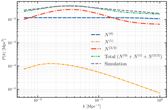
Figure 6: Contributions to the KSZ reconstruction noise, computed as described in §VI.4. The reconstruction noise in simulations agrees well with the sum of analytic contributions $(N^{(0)}+N^{(1)}+N^{(3/2)})$. All noise power spectra have been angle-averaged over ${\bf k}$, and $N^{(1)}$ and $N^{(3/2)}$ have been computed using approximations which are valid for $k\rightarrow 0$.

The preceding results have assumed fiducial survey parameters from §III. In this paper, we will not explore dependence on galaxy density $n_{g}$ or redshift $z$, although this should be fairly straightforward using our expressions for $N^{(0)}$ and $N^{(3/2)}$ bias. However, one parameter which is easy to analyze is the CMB noise level. In the approximation (81), the $N^{(3/2)}$-bias is independent of the CMB noise. On the other hand, Eq. (26) shows that the $N^{(0)}$-bias is proportional to $C_{l}^{\rm tot}=(C_{l}+N_{l})$ evaluated on kSZ scales $l\sim 5000$. Therefore, as the CMB experiment becomes more sensitive, the $N^{(3/2)}$-bias becomes more important, relative to $N^{(0)}$.

Since our simulations use futuristic CMB noise parameters (0.5 $\mu$K-arcmin, $\theta_{\rm fwhm}$ = 1 arcmin), and galaxy survey parameters comparable to DESI, it seems likely that $N^{(3/2)}$ will be small (relative to $N^{(0)}$) for DESI in combination with near-future CMB experiments such as Simons Observatory. However, if DESI is replaced by an experiment with larger galaxy density (e.g. Rubin Observatory), or if the CMB noise is $\lesssim 1$ $\mu$K-arcmin, then $N^{(3/2)}$ may be important.

VII Recovering $f_{NL}$ with an MCMC pipeline

In this section, we develop an MCMC-based analysis pipeline which recovers the value of $f_{NL}$ from a galaxy catalog and CMB map. We demonstrate the ability of our pipeline to recover the correct value of $f_{NL}$, and validate its statistical errors with Monte Carlo simulations.

In our pipeline, $f_{NL}$ sensitivity arises entirely from $f_{NL}$ dependence of the galaxy bias: $b(k)=b_{g}+f_{NL}b_{ng}/k^{2}$. The velocity reconstruction ${\hat{v}_{r}}$ is not directly $f_{NL}$-sensitive. However, ${\hat{v}_{r}}$ can be used to cancel sample variance in the galaxy field, thus improving the statistical error on $f_{NL}$ relative to a measurement of $\delta_{g}$ alone. The idea of sample variance cancellation was introduced by Seljak in Seljak (2009). Sample variance cancellation is automatically incorporated by our MCMC pipeline, since we write down the full posterior likelihood ${\mathcal{L}}(f_{NL}|\delta_{g},{\hat{v}_{r}})$ (Eq. (89) below), which includes sample variance cancellation automatically.

When constructing our posterior likelihood, we assume that the reconstruction noise power spectrum is given by the $N^{(0)}$-bias in Eq. (26). This neglects the $N^{(3/2)}$ bias, even though we have shown that $N^{(3/2)}$ is comparable to $N^{(0)}$ for our fiducial survey parameters. In principle, neglecting $N^{(3/2)}$ can produce both biased $f_{NL}$ estimates and underestimated statistical errors (as in the CMB lensing case). However, in this section we will find that within statistical errors of our simulations, our MCMC pipeline recovers unbiased estimates of $f_{NL}$, with scatter consistent with a Fisher matrix forecast.

In our pipeline, we have perfect knowledge of the galaxy-electron power spectrum $P_{ge}(k_{S})$, and therefore we expect the reconstruction bias $b_{v}$ to equal 1. However, in our MCMC’s, we will include $b_{v}$ as a nuisance parameter and marginalize it, so that our analysis is more representative of real experiments. As a consistency check, we expect the value of $b_{v}$ recovered from the MCMC’s to be consistent with 1.

VII.1 MCMC pipeline description

The inputs to our pipeline are a realization $\delta_{h}({\bf k})$ of the 3-d halo field, and the kSZ velocity reconstruction ${\hat{v}_{r}}({\bf k})$. We want to constrain the cosmological parameter $f_{NL}$, and the nuisance parameters $b_{g},b_{v}$. Here, $b_{g}$ is the Gaussian halo bias, and $b_{v}$ is the kSZ velocity reconstruction bias from §V.2. For notational compactness, let $\pi$ denote the three-component parameter vector $\pi=(f_{NL},b_{g},b_{v})$.

We start by writing down the two-point statistics of the fields $\delta_{g}$ and ${\hat{v}_{r}}$. For each Fourier mode ${\bf k}$, let $\theta({\bf k})$ be the two-component vector of fields:

$$\theta({\bf k})=\left(\begin{array}[]{c}\delta_{h}({\bf k})\\ {\hat{v}_{r}}({\bf k})\end{array}\right)$$ (82)

Let $C({\bf k},\pi)$ be the 2-by-2 Hermitian matrix defined by:

$$\big{\langle}\theta({\bf k})\,\theta({\bf k}^{\prime})^{\dagger}\big{\rangle}=C({\bf k},\pi)\,(2\pi)^{3}\delta^{3}({\bf k}-{\bf k}^{\prime})$$ (83)

We model $C({\bf k},\pi)$ on large scales by:

$$C_{11}(k,\pi) = b_{h}(k,\pi)^{2}P_{\rm lin}(k)+\frac{1}{n_{h}}$$ (84)

$$C_{12}({\bf k},\pi) = -ik_{r}\left(\frac{faH}{k^{2}}\right)\,b_{v}\,b_{h}(k,\pi)P_{\rm lin}(k)$$ (85)

$$C_{22}({\bf k},\pi) = k_{r}^{2}\left(\frac{faH}{k^{2}}\right)^{2}\,b_{v}^{2}\,P_{\rm lin}(k)+N_{v_{r}}^{(0)}({\bf k})$$ (86)

where $b_{h}(k,\pi)$ is the non-Gaussian halo bias:

$$b_{h}(k,\pi)=b_{g}+f_{NL}\frac{2\delta_{c}(b_{g}-1)}{\alpha(k,z)}\hskip 28.45274pt(\delta_{c}=1.42)$$ (87)

and $N^{(0)}_{v_{r}}({\bf k})$ was given in Eq. (26). The model for $C({\bf k},\pi)$ in Eqs. (84)–(86) follows if we assume that $\delta_{h}$ and ${\hat{v}_{r}}$ are modeled as:

$$\delta_{h}({\bf k}) = b_{h}(k)\,\delta_{m}({\bf k})+\mbox{(Poisson noise)}$$

$${\hat{v}_{r}}({\bf k}) = ib_{v}k_{r}\frac{faH}{k}\delta_{m}({\bf k})+\mbox{(Reconstruction noise)}$$ (88)

In the previous section, we tested these assumptions systematically, thus validating our model (84)–(86) for the two-point function $C({\bf k},\pi)$.

However, to run an MCMC we need to go beyond the two-point function, by writing down a model for the posterior likelihood ${\mathcal{L}}(\pi|\theta)$ for parameter vector $\pi$, given data realization $\theta({\bf k})$. Here, we simply assume the Gaussian likelihood derived from the two-point function in Eqs. (84)–(86):

$${\mathcal{L}}\big{(}\pi|\theta)\propto\prod_{\bf k}\big{(}\mbox{Det}\,C({\bf k},\pi)\big{)}^{-1/2}\exp\left(-\frac{\theta({\bf k})^{\dagger}C({\bf k},\pi)^{-1}\theta({\bf k})}{2V}\right)$$ (89)

where the survey volume $V$ on the RHS arises from our finite-volume Fourier convention in Eq. (7). This “field-level” likelihood function makes fewer approximations than a likelihood function based on power spectrum bandpowers. However, we emphasize that the likelihood (89) treats $\delta_{g}$ and ${\hat{v}_{r}}$ as Gaussian fields, and results from previous sections do not imply its validity. Indeed, the main purpose of this section is to validate the Gaussian likelihood function, by showing that it leads to valid constraints on $f_{NL}$.

We truncate the likelihood (89) at $k_{\rm max}=0.012$ Mpc^-1. The posterior likelihood is sampled using Goodman-Weare sampling algorithm Goodman and Weare (2010) implemented in the public library emcee Foreman-Mackey et al. (2013). We use flat priors over a reasonable range of values for all three model parameters of the model, and run the chain long enough to fulfil recommended convergence criterion based on correlation length.

VII.2 Unbiased $f_{NL}$ estimates from MCMC

We now present results from running our MCMC pipeline on $N$-body simulations. First, we check for additive bias in $f_{NL}$, by confirming that when the MCMC pipeline is run on simulations with $f_{NL}=0$, there is no bias toward positive or negative $f_{NL}$.

Figure 7: MCMC posteriors on $(b_{g},f_{nl})$ from combined analysis of 100 high resolution Quijote simulations with $f_{NL}=0$. The three likelihoods correspond to MCMC analysis of the halo field alone ($\delta_{h}$), joint analysis of the halo field and kSZ velocity reconstruction ($\delta_{h},{\hat{v}_{r}}$), and joint analysis of the halo field and the noise-free matter field ($\delta_{h},\delta_{m}$). In the second case $(\delta_{h},{\hat{v}_{r}})$, likelihoods have been marginalized over the additional nuisance parameter $b_{v}$.

In Figure 7, we jointly analyze all 100 Quijote simulations with $f_{NL}=0$, by multiplying together their posterior likelihoods. We run three versions of the MCMC pipeline as follows. First, we constrain parameters using the halo field alone $(\delta_{h})$. Second, we use our standard setup described in the previous section, where we include the halo field and the kSZ velocity reconstruction $(\delta_{h}+{\hat{v}_{r}})$. Third, we use the halo field and a perfect, noise-free realization of the matter overdensity $(\delta_{h}+\delta_{m})$. Note that in the second case $(\delta_{h}+{\hat{v}_{r}})$, the MCMC parameters are $(f_{NL},b_{g},b_{v})$, whereas in the first and third cases, the parameters are $(f_{NL},b_{g})$. In the second case $(\delta_{h}+{\hat{v}_{r}})$, the likelihoods in Figure 7 are marginalized over the additional parameter $b_{v}$.

The $f_{NL}$ constraint in Figure 7 from $(\delta_{h}+{\hat{v}_{r}})$ is significantly better than the $\delta_{h}$-only constraint, and slightly worse than the $(\delta_{h}+\delta_{m})$-constraint. This shows that sample variance cancellation between $\delta_{h}$ and ${\hat{v}_{r}}$ is happening, and the level of cancellation is comparable to what would be obtained from a perfect measurement of $\delta_{m}$.

From Figure 7, we can also conclude that the $f_{NL}$ estimates from our MCMC pipeline are not additively biased. The combined $(\delta_{h}+{\hat{v}_{r}})$ likelihood is consistent with $f_{NL}=0$, within the statistical error from 100 simulations. Any additive $f_{NL}$ bias must be smaller than this statistical error (roughly $\Delta f_{NL}=2$).

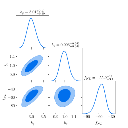
Figure 8: MCMC constraints for $f_{nl}=-50$ (top panel) and $f_{NL}=50$ (bottom). Each panel combines likelihoods from four $N$-body simulations, each with volume 1 $h^{-3}$ Gpc³. The recovered $f_{NL}$ values are consistent with the true values, within statistical errors.

Next, we check for multiplicative bias in $f_{NL}$, by analyzing simulations with $f_{NL}\neq 0$ and confirming that we recover the correct value of $f_{NL}$. In Figure 8, we present results from non-Gaussian $N$-body simulations with $f_{NL}=\pm 50$. It is seen that the MCMC pipeline recovers the correct value of $f_{NL}$ within its reported statistical error (around 10–20%). The total simulation volume is smaller (8 $h^{-3}$ Gpc³) here than in the $f_{NL}=0$ case (100 $h^{-3}$ Gpc³), where Quijote simulations are available. Therefore, we cannot characterize the behavior of the MCMC pipeline as precisely as we can in the $f_{NL}=0$ case. However, the current observational situation is that $f_{NL}$ has not been detected, and the priority for upcoming experiments will be testing the null hypothesis that $f_{NL}=0$. In this situation, it should suffice to have a precise characterization of the pipeline on simulations with $f_{NL}=0$, and a $\approx$10-20% test for bias on simulations with nonzero $f_{NL}$.

VII.3 Consistency between MCMC results and Fisher matrix forecasts

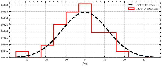
Figure 9: A test of the error estimates from our MCMC pipeline. The solid histogram contains one $f_{NL}$ estimate from each of 100 high-res Quijote simulations with $f_{NL}=0$, obtained by taking the median of the $f_{NL}$ posterior likelihood (after marginalizing over $b_{g},b_{v}$). The dashed line is a Gaussian whose width is equal to the Fisher forecasted error on $f_{NL}$. The two distributions have equal widths, within statistical errors from 100 simulations.

The tests in the previous section show that the MCMC pipeline recovers unbiased estimates of $f_{NL}$, but do not test statistical errors on $f_{NL}$ inferred from the posteriors. In this section, we will validate $f_{NL}$ errors from the MCMC pipeline.

For the sake of discussion, we briefly describe a completely rigorous, Bayesian procedure for validating $f_{NL}$ errors (even though this is not what we will end up doing!) Suppose we choose a prior $p(f_{NL})$, and generate a large number of simulations with $f_{NL}$ values sampled from the prior. For each simulation $s$, we use MCMC to compute the posterior likelihood $p(f_{NL}|s)$, and rank the true value of $f_{NL}$ within the posterior likelihood, to obtain a quantile $0<q<1$. Then we should find that $q$ is uniform distributed, if the posterior likelihoods have been computed correctly. This is a precise statement that can be proved rigorously. This check validates error estimates from the MCMC pipeline, in the sense that if the MCMC pipeline overestimates its error bars (i.e. returns posterior likelihoods which are too wide), then the distribution of $q$-values will be narrower than uniform.

The difficulty with this method is that it would require many simulations with $f_{NL}\neq 0$, which would be very expensive. Instead, we will use an alternative method which uses only simulations with $f_{NL}=0$ (so that we can use the Quijote simulations). For each such simulation, let $f_{NL}^{\rm med}$ be the median of the MCMC posterior likelihood for $f_{NL}$ (marginalized over $b_{g},b_{v}$). Let $\sigma(f_{NL}^{\rm med})$ be the RMS scatter in $f_{NL}^{\rm med}$ over 100 Quijote simulations. We will compare $\sigma(f_{NL}^{\rm med})$ to the Fisher forecasted statistical error on $f_{NL}$ (which we will denote $\sigma_{F}(f_{NL})$). Intuitively, we expect that $\sigma(f_{NL}^{\rm med})\approx\sigma_{F}(f_{NL})$, but this is not rigorously guaranteed, so this test is not quite as precise as the Bayesian test described above. However, the Cramér-Rao inequality implies $\sigma(f_{NL}^{\rm med})\geq\sigma_{F}(f_{NL})$.

We briefly describe the implementation of our Fisher matrix forecast. The 3-by-3 Fisher matrix is given by:

$$F_{ab}=\frac{1}{2}\sum_{{\bf k}}\mbox{Tr}\left[C({\bf k},\pi)^{-1}\frac{\partial C({\bf k},\pi)}{\partial\pi_{a}}C({\bf k},\pi)^{-1}\frac{\partial C({\bf k},\pi)}{\partial\pi_{b}}\right]$$ (90)

where $a,b$ index elements of the parameter vector $(\pi_{1},\pi_{2},\pi_{3})=(f_{NL},b_{g},b_{v})$. The 2-by-2 covariance matrix $C({\bf k},\pi)$ was defined previously in Eqs. (84)–(86), and parameter derivatives of $C$ are straightforward to compute. The Fisher-forecasted statistical error on $f_{NL}$, marginalized over $(b_{g},b_{v})$, is given by $\sigma_{F}(f_{NL})=\sqrt{(F^{-1})_{11}}$.

In Figure 9, the solid histogram shows values of $f_{NL}^{\rm med}$ for all 100 Quijote simulations. The dashed curve is a Gaussian whose width is equal to the Fisher forecasted error on $f_{NL}$. We find that $\sigma(f_{NL}^{\rm med})=10.54$ and $\sigma_{F}(f_{NL})=11.54$. These values are equal (at $2\sigma$) within statistical errors from 100 Quijote simulations. This agreement was not guaranteed in advance, since the Fisher forecast makes approximations (neglecting $N^{(3/2)}$-bias, treating $\delta_{g}$ and ${\hat{v}_{r}}$ as Gaussian fields), whereas $\sigma(f_{NL}^{\rm med})$ is a Monte Carlo error estimate based on $N$-body simulations. The observed agreement directly valdiates previous Fisher forecasts based on kSZ velocity reconstruction (e.g. Smith et al. (2018); Münchmeyer et al. (2019)).

VIII Discussion

KSZ velocity reconstruction is a promising method for constraining cosmology. However, almost all work to date (with the notable exception of Cayuso et al. (2018)) has been based on analytic modeling which has not been tested with simulations. In this paper, we have made a detailed comparison between analytic models and $N$-body simulations. Overall, we have found good agreement, concluding with an end-to-end pipeline which recovers unbiased estimates of $f_{NL}$ from simulated galaxy and kSZ datasets, with statistical errors which are consistent with a Fisher matrix forecast. This initial study is a starting point for future refinements, and we list some possibilities here:

• We have found a discrepancy between velocity reconstruction noise in our $N$-body simulations, and the kSZ $N^{(0)}$-bias which is typically used in forecasts. Using the halo model, we revisited the calculation of the reconstruction noise power spectrum, and found new terms: the kSZ $N^{(1)}$ and $N^{(3/2)}$ biases. We computed these terms numerically and found that $N^{(1)}$ is negligible, while $N^{(3/2)}$ matches the excess noise seen in simulations (Figure 6). Our final expression for $N^{(3/2)}$ (Eq. (81)) is algebraically simple enough that it should be straightforward to include in future forecasts or data analysis.

• Similarly, we have found that the non-Gaussian bandpower covariance of the reconstruction noise can be large (§V.3). It would be interesting to model this effect, e.g. using the halo model.

  For our choice of fiducial survey parameters (§III), neither the non-Gaussian bandpower covariance nor the $N^{(3/2)}$-bias has much impact on the bottom-line $f_{NL}$ constraint. However, this may not be the case for other choices of survey parameters (CMB noise, galaxy density, redshift, etc.), and systematic exploration of parameter dependence would be valuable.

• We have used collisionless $N$-body simulations, making the approximations that electrons trace dark matter ($\delta_{e}=\delta_{m}$) and galaxies are in one-to-one correspondence with dark matter halos ($\delta_{g}=\delta_{h}$). These are crude approximations, and our simulations overpredict the small-scale galaxy-electron power spectrum $P_{ge}(k_{S})$ by an order-one factor. We do not think this is an issue for purposes of this paper, where our goal is to test agreement between simulations and theory under self-consistent assumptions. However, it would be good to check this by incorporating baryonic physics, for example using the Illustris-TNG simulation Nelson et al. (2018).

• We have used a snapshot geometry (§II.1), which could be generalized to a lightcone geometry with redshift evolution.

• We have not included CMB foregrounds and other non-Gaussian secondaries (e.g. lensing). This issue is not as serious as it sounds, since there are symmetry arguments which show that the velocity reconstruction bias produced by foregrounds and secondaries should be small.

  In the case of CMB lensing, there is a symmetry which reverses the sign of the primary CMB anisotropy $T_{\rm pri}\rightarrow-T_{\rm pri}$ while leaving late-universe LSS unchanged. Strictly speaking, this is an approximate symmetry which assumes that the last scattering surface and the late universe are statistically independent, but this is an excellent approximation on small scales. Under this symmetry, the lensed CMB is odd ($T_{\rm len}\rightarrow-T_{\rm len})$, whereas the kSZ and other secondaries/foregrounds are even ($T\rightarrow T$). This implies that lensing cannot produce a velocity reconstruction bias $\langle{\hat{v}_{r}}\rangle$.

  Most non-kSZ secondaries (including CMB lensing, but also e.g. tSZ or CIB) are even under radial reflection symmetry, whereas the kSZ is odd. This implies that there is no velocity reconstruction bias. However, radial reflection is only an approximate symmetry in a lightcone geometry (unlike the snapshot geometry where it is exact), so there will be some residual bias which should be quantified with simulations. Additionally, even if foregrounds/secondaries produce minimal velocity reconstruction bias, their non-Gaussian statistics may produce extra reconstruction noise (relative to a Gaussian field), and it would be useful to quantify this with simulations.

• A natural extension of this work would be to study the effect of redshift space distortions (RSD’s) or photometric redshift errors. Ref. Smith et al. (2018) makes analytic predictions for the effect of RSD’s and photo-$z$ errors on kSZ velocity reconstruction, on large scales and assuming a simplified photo-$z$ model. It would be interesting to compare these predictions to simulations. Additionally, simulations could be used to study small-scale RSD’s (“Fingers of God”) and catastrophic photo-$z$ errors, where analytic predictions are difficult.

  If RSD’s are included in the simulations, then it should be possible to break the kSZ optical depth degeneracy, as first proposed in Sugiyama et al. (2017). More precisely, the $\langle gv_{r}\rangle$ correlation function contains terms proportional to $\mu^{0}$ and $\mu^{2}$, and by comparing the amplitude of these terms, the parameter combination $f/b_{g}$ can be constrained, with no contribution from $b_{v}$. It would be very interesting to test this picture with simulations.

• We have focused on constraining $f_{NL}$, and it would be interesting to study other applications of kSZ tomography, for example using sample variance cancellation to constrain the RSD parameter $f=\partial\log D/\partial\log a$. Similarly, we could generalize the non-Gaussian model, by introducing scale-dependent $f_{NL}$, or the “$g_{NL}$ model” with $\zeta^{3}$-type non-Gaussianity.

Appendix A Diagrammatic rules for the halo model

The main purpose of this appendix is to derive Eqs. (56)–(66) for the non-Gaussian six-point function

$$\big{\langle}\delta_{g}({\bf k}_{1})\delta_{e}({\bf k}_{2})\delta_{g}({\bf k}_{3})\delta_{e}({\bf k}_{4})v_{r}({\bf k}_{5})v_{r}({\bf k}_{6})\big{\rangle}_{ng}$$ (91)

in the halo model. In general, $n$-point correlation functions in the halo model consist of many combinatorial terms. A second purpose of this appendix is to show that these terms can be enumerated using diagrammatic rules, similar to Feynman rules in QFT.

We consider the simplest version of the halo model, in which halos are linearly biased tracers of a Gaussian field $\delta_{\rm lin}$ (the linear density field). In this model, the expected number of halos per volume per unit halo mass is:

$$s(M,{\bf x})=n(M)\big{(}1+b(M)\delta_{\rm lin}({\bf x})\big{)}$$ (92)

where $n(M)$ is the halo mass function and $b(M)$ is the linear bias. We will call $s(M,{\bf x})$ the halo source field, and distingiush it from the halo density field $\delta_{h}({\bf x})$, which is a sum of delta functions. By assumption in the halo model, the halo density field is given by Poisson-sampling the halo source field.

We consider fields $\delta_{X}$ which are sums over halos:

$$\delta_{X}({\bf k})=\sum_{j}W_{X}(M_{j},k)e^{-i{\bf k}\cdot{\bf x}_{j}}$$ (93)

where the $j$-th halo has mass $M_{j}$ and position ${\bf x}_{j}$. In particular, in our collisionless approximation (§III.1), the electron field $\delta_{e}$ and galaxy field $\delta_{g}$ are of the form (93), with weight functions $W_{X}(M,z)$ given by:

$$W_{e}(M,k)=\frac{M}{\rho_{m}}u_{M}(k)\hskip 42.67912ptW_{g}(M,k)=\left\{\begin{array}[]{cl}1/n_{h}&\mbox{ if }M\geq M_{\rm min}\\ 0&\mbox{ if }M<M_{\rm min}\end{array}\right.$$ (94)

where $u_{M}(k)$ is the Fourier-transformed density profile of a halo of mass $M$, normalized so that $u_{M}(0)=1$.

A.1 Expectation values in a fixed realization of the halo source field

Expectation values in the halo model can be calculated in two steps. First, we take an “inner” average over Poisson-sampled halos, in a fixed realization of the source field $s(M,{\bf x})$. Second, we take an “outer” average over realizations of $s(M,{\bf x})$, or equivalently realizations of $\delta_{\rm lin}({\bf x})$ via Eq. (92). In this section, we will analyze the inner average. We consider an $n$-point expectation value $\langle\delta_{X_{1}}({\bf k}_{1})\cdots\delta_{X_{n}}({\bf k}_{n})\rangle_{s}$, where the suffix $\langle\cdot\rangle_{s}$ means that the expectation value is taken over Poisson placements of halos, in a fixed realization of $s(M,{\bf x})$.

We plug in the definition (93) of $\delta_{X}$, to write the expectation value as a sum over $n$-tuples of halos:

$$\big{\langle}\delta_{X_{1}}({\bf k}_{1})\cdots\delta_{X_{n}}({\bf k}_{n})\big{\rangle}_{s}=\left\langle\sum_{j_{1},\cdots,j_{n}}\left(\prod_{i=1}^{n}W_{X_{i}}(M_{j_{i}},k_{i})e^{-i{\bf k}_{i}\cdot{\bf x}_{j_{i}}}\right)\right\rangle_{s}$$ (95)

Then, as usual in the halo model, we split the sum into combinatorial terms, based on which elements of the $n$-tuple $(j_{1},\cdots,j_{n})$ are equal to each other. For example, consider the four-point function

$$\big{\langle}\delta_{g}({\bf k}_{1})\delta_{e}({\bf k}_{2})\delta_{g}({\bf k}_{3})\delta_{e}({\bf k}_{4})\big{\rangle}$$ (96)

which is a subset of the six-point function (91). Writing the four-point function as a sum over halo quadruples, we could keep terms $(j_{1},j_{2},j_{3},j_{4})$ such that

$$j_{1}=j_{4}=j\hskip 14.22636pt\mbox{and}\hskip 14.22636ptj_{2}=j_{3}=j^{\prime}\hskip 14.22636pt\mbox{with $j\neq j^{\prime}$}$$ (97)

obtaining a contribution which we will denote by $T$:

$$T=\left\langle\sum_{j\neq j^{\prime}}\Big{(}W_{g}(M_{j},k_{1})W_{e}(M_{j},k_{4})e^{-i({\bf k}_{1}+{\bf k}_{4})\cdot{\bf x}_{j}}\Big{)}\Big{(}W_{e}(M_{j^{\prime}},k_{2})W_{g}(M_{j^{\prime}},k_{3})e^{-i({\bf k}_{2}+{\bf k}_{3})\cdot{\bf x}_{j^{\prime}}}\Big{)}\right\rangle_{s}$$ (98)

This term $T$ is one of 7 “two-halo” terms which contribute to the four-point function (96), out of 15 total terms. Physically, $T$ corresponds to summing over all quadruples $(g_{1},e_{2},g_{3},e_{4})$ such that galaxy $g_{1}$ and electron $e_{4}$ are in one halo, and galaxy $g_{2}$ and electron $e_{3}$ are in a different halo. To compute $T$, we replace each sum $\sum_{j}$ by an integral $\int d^{3}{\bf x}\,dM\,s(M,{\bf x})$, obtaining:

$$T =\left(\int d^{3}{\bf x}\,dM\,W_{g}(M,k_{1})W_{e}(M,k_{4})s(M,{\bf x})e^{-i({\bf k}_{1}+{\bf k}_{4})\cdot{\bf x}}\right)$$

$$\hskip 14.22636pt\times\left(\int d^{3}{\bf x}^{\prime}\,dM^{\prime}\,W_{e}(M^{\prime},k_{2})W_{g}(M^{\prime},k_{3})s(M^{\prime},{\bf x}^{\prime})e^{-i({\bf k}_{2}+{\bf k}_{3})\cdot{\bf x}^{\prime}}\right)$$

$$=\left(\int dM\,W_{g}(M,k_{1})W_{e}(M,k_{4})s(M,{\bf k}_{1}+{\bf k}_{4})\right)\left(\int dM^{\prime}\,W_{e}(M^{\prime},k_{2})W_{g}(M^{\prime},k_{3})s(M,{\bf k}_{2}+{\bf k}_{3})\right)$$ (99)

We now introduce diagrammatic notation, representing this equation by the diagram:

$$T=\left(\leavevmode\hbox{$\vbox{\hbox{\resizebox{}{}{{\leavevmode\hbox{\set@color{ \leavevmode\hbox to19pt{\vbox to59.02pt{\text{[drawing]}}}}}}}}}$}\right) M \delta_{g}({\bf k}_{1}) \delta_{e}({\bf k}_{4}) M^{\prime} \delta_{e}({\bf k}_{2}) \delta_{g}({\bf k}_{3}) M \delta_{g}({\bf k}_{1}) \delta_{e}({\bf k}_{4}) M^{\prime} \delta_{e}({\bf k}_{2}) \delta_{g}({\bf k}_{3})$$ (100)

where diagrams are translated to equations using the rules:

$$\leavevmode\hbox{$\vbox{\hbox{\resizebox{}{}{{\leavevmode\hbox{\set@color{ \leavevmode\hbox to70.51pt{\vbox to54.29pt{\text{[drawing]}}}}}}}}}$}=\int dM\,s(M,\mathop{\textstyle\sum}\limits{\bf k}_{i})\hskip 35.56593pt\leavevmode\hbox{$\vbox{\hbox{\resizebox{}{}{{\leavevmode\hbox{\set@color{ \leavevmode\hbox to54.65pt{\vbox to33.17pt{\text{[drawing]}}}}}}}}}$}=W_{X}(M,k) \cdots {\bf k}_{1} {\bf k}_{2} {\bf k}_{n} M M \delta_{X}({\bf k}) \cdots {\bf k}_{1} {\bf k}_{2} {\bf k}_{n} M M \delta_{X}({\bf k})$$ (101)

In general, an $n$-point correlation function $\langle\delta_{X_{i}}({\bf k}_{i})\cdots\delta_{X_{n}}({\bf k}_{n})\rangle_{s}$ is the sum over all diagrams obtained using these rules. External lines in the diagrams correspond to fields being correlated, and vertices correspond to halos.

A.2 Fully averaged expectation values

The diagrammatic rules just derived in Eq. (101) correspond to an expectation value $\langle\cdot\rangle_{s}$ over Poisson placements of halos, in a fixed realization of the halo source field $s(M,{\bf x})$. In this section, we take the “outer” expectation value over $s$. We also consider $n$-point functions which contain factors of the linear density field $\delta_{\rm lin}({\bf k})$, or the radial velocity $v_{r}({\bf k})$, so that our machinery will be general enough to calculate the six-point function (91).

In general, the source function $s(M,{\bf x})$ will depend on the halo bias model. We will consider the simplest possibility, namely the linear bias model $s(M,{\bf x})=n(M)(1+b(M)\delta_{\rm lin}({\bf x}))$, or equivalently in Fourier space:

$$s(M,{\bf k})=n(M)\Big{[}(2\pi)^{3}\delta^{3}({\bf k})+b(M)\delta_{\rm lin}({\bf k})\Big{]}$$ (102)

Now consider a quantity which depends on the halo source field $s(M,{\bf k})$, such as the term $T$ from the previous section:

$$T=\int dM\,dM^{\prime}\,W_{g}(M,k_{1})W_{e}(M,k_{4})W_{e}(M^{\prime},k_{2})W_{g}(M^{\prime},k_{3})\,\Big{[}s(M,{\bf k}_{1}+{\bf k}_{4})s(M,{\bf k}_{2}+{\bf k}_{3})\Big{]}$$ (103)

To average over $s$, we replace all factors of $s$ by the RHS of Eq. (102), and take the expectation value over $\delta_{\rm lin}$ using Wick’s theorem. This gives:

$$\langle T\rangle =\int dM\,dM^{\prime}\,W_{g}(M,k_{1})W_{e}(M,k_{4})W_{e}(M^{\prime},k_{2})W_{g}(M^{\prime},k_{3})n(M)n(M^{\prime})$$

$$\hskip 28.45274pt\times\Big{[}(2\pi)^{6}\delta^{3}({\bf k}_{1}+{\bf k}_{2})\delta^{3}({\bf k}_{3}+{\bf k}_{4})+b(M)b(M^{\prime})(2\pi)^{3}\delta^{3}(\mathop{\textstyle\sum}\limits{\bf k}_{i})\Big{]}$$ (104)

Diagramatically, we represent this procedure for averaging over $s$ as follows. We start with the diagram (100) representing $T$, in which each hollow circle contains one factor of $s(M,{\bf k})$. We sum over all ways of either pairing vertices with wavy lines (representing a Wick contraction proportional to $P_{\rm lin}$), or leaving vertices unpaired. In the case of $T$, there are two possibilities:

          (105)

where the diagrams are interpreted using the following diagrammatic rules:

(106)

Note that we use hollow vertices in diagrams where $s$ is not averaged (Eq. (101)), and solid vertices in diagrams where $s$ is averaged (Eq. (106)).

A $n$-point expectation value of the form $\langle\delta_{X_{i}}({\bf k}_{1})\cdots\delta_{X_{n}}({\bf k}_{n})\rangle$ may be computed by enumerating all diagrams, using the preceding diagrammatric rules. An $n$-point function which also contains factors of $\delta_{\rm lin}({\bf k})$ or $v_{r}({\bf k})$, such as the six-point function (91), can be represented diagrammatically by adding the following external lines:

$$\leavevmode\hbox{$\vbox{\hbox{\resizebox{}{}{{\leavevmode\hbox{\set@color{ \leavevmode\hbox to30.39pt{\vbox to33.74pt{\text{[drawing]}}}}}}}}}$}=P_{\rm lin}(k)\hskip 56.9055pt\leavevmode\hbox{$\vbox{\hbox{\resizebox{}{}{{\leavevmode\hbox{\set@color{ \leavevmode\hbox to27.61pt{\vbox to33.74pt{\text{[drawing]}}}}}}}}}$}=\frac{ik_{r}}{k}P_{mv}(k) \delta_{\rm lin}({\bf k}) v_{r}({\bf k}) \delta_{\rm lin}({\bf k}) v_{r}({\bf k})$$ (107)

where we have assumed that $v_{r}({\bf k})$ is evaluated on a linear scale, so that $v_{r}({\bf k})=(ik_{r}/k)v({\bf k})=(ik_{r}/k)(faH/k)\delta_{\rm lin}({\bf k})$.

A.3 The six-point function $\langle\delta_{g}^{2}\delta_{e}^{2}v_{r}^{2}\rangle$

We calculate the non-Gaussian six-point function (91) using the diagrammatic rules in Eqs. (106), (107). Up to permutations of external legs, there are five possible diagrams:

$$D_{1} =\left(\leavevmode\hbox{$\vbox{\hbox{\resizebox{}{}{{\leavevmode\hbox{\set@color{ \leavevmode\hbox to0pt{\vbox to0pt{\text{[drawing]}}}}}}}}}$}\right) \delta_{g}({\bf k}_{1}) \delta_{e}({\bf k}_{2}) v_{r}({\bf k}_{5}) \delta_{g}({\bf k}_{3}) \delta_{e}({\bf k}_{4}) v_{r}({\bf k}_{6}) \delta_{g}({\bf k}_{1}) \delta_{e}({\bf k}_{2}) v_{r}({\bf k}_{5}) \delta_{g}({\bf k}_{3}) \delta_{e}({\bf k}_{4}) v_{r}({\bf k}_{6}) D_{2} =\left(\leavevmode\hbox{$\vbox{\hbox{\resizebox{}{}{{\leavevmode\hbox{\set@color{ \leavevmode\hbox to30.41pt{\vbox to16.67pt{\text{[drawing]}}}}}}}}}$}\right) \delta_{e}({\bf k}_{2}) \delta_{g}({\bf k}_{3}) \delta_{e}({\bf k}_{4}) \delta_{g}({\bf k}_{1}) v_{r}({\bf k}_{5}) v_{r}({\bf k}_{6}) \delta_{e}({\bf k}_{2}) \delta_{g}({\bf k}_{3}) \delta_{e}({\bf k}_{4}) \delta_{g}({\bf k}_{1}) v_{r}({\bf k}_{5}) v_{r}({\bf k}_{6})$$

$$D_{3} =\left(\leavevmode\hbox{$\vbox{\hbox{\resizebox{}{}{{\leavevmode\hbox{\set@color{ \leavevmode\hbox to0pt{\vbox to0pt{\text{[drawing]}}}}}}}}}$}\right) \delta_{g}({\bf k}_{1}) \delta_{e}({\bf k}_{2}) \delta_{g}({\bf k}_{3}) \delta_{e}({\bf k}_{4}) v_{r}({\bf k}_{5}) v_{r}({\bf k}_{6}) \delta_{g}({\bf k}_{1}) \delta_{e}({\bf k}_{2}) \delta_{g}({\bf k}_{3}) \delta_{e}({\bf k}_{4}) v_{r}({\bf k}_{5}) v_{r}({\bf k}_{6}) D_{4} =\left(\leavevmode\hbox{$\vbox{\hbox{\resizebox{}{}{{\leavevmode\hbox{\set@color{ \leavevmode\hbox to0pt{\vbox to0pt{\text{[drawing]}}}}}}}}}$}\right) \delta_{g}({\bf k}_{1}) \delta_{e}({\bf k}_{2}) \delta_{g}({\bf k}_{3}) \delta_{e}({\bf k}_{4}) v_{r}({\bf k}_{5}) v_{r}({\bf k}_{6}) \delta_{g}({\bf k}_{1}) \delta_{e}({\bf k}_{2}) \delta_{g}({\bf k}_{3}) \delta_{e}({\bf k}_{4}) v_{r}({\bf k}_{5}) v_{r}({\bf k}_{6})$$

$$D_{5} =\left(\leavevmode\hbox{$\vbox{\hbox{\resizebox{}{}{{\leavevmode\hbox{\set@color{ \leavevmode\hbox to29.57pt{\vbox to16.67pt{\text{[drawing]}}}}}}}}}$}\right) \delta_{g}({\bf k}_{1}) \delta_{e}({\bf k}_{2}) \delta_{g}({\bf k}_{3}) v_{r}({\bf k}_{5}) v_{r}({\bf k}_{6}) \delta_{e}({\bf k}_{4}) \delta_{g}({\bf k}_{1}) \delta_{e}({\bf k}_{2}) \delta_{g}({\bf k}_{3}) v_{r}({\bf k}_{5}) v_{r}({\bf k}_{6}) \delta_{e}({\bf k}_{4})$$ (108)

In particular, there are no fully connected diagrams, as claimed in the main text (§VI.3). We evaluate these diagrams as follows (denoting ${\bf k}_{i_{1}\cdots i_{n}}=({\bf k}_{i_{1}}+\cdots+{\bf k}_{i_{n}})$):

$$D_{1} =\left(\int dM\,n(M)b(M)W_{g}(M,k_{1})W_{e}(M,k_{2})\frac{ik_{5r}}{k_{5}}P_{mv}(k_{5})\,(2\pi)^{3}\delta^{3}({\bf k}_{125})\right)$$

$$\hskip 42.67912pt\times\left(\int dM^{\prime}\,n(M^{\prime})b(M^{\prime})W_{g}(M^{\prime},k_{3})W_{e}(M^{\prime},k_{4})\frac{ik_{6r}}{k_{6}}P_{mv}(k_{6})\,(2\pi)^{3}\delta^{3}({\bf k}_{346})\right)$$

$$=-\beta_{1}(k_{2})\beta_{1}(k_{4})\frac{k_{5r}k_{6r}}{k_{5}k_{6}}P_{mv}(k_{5})P_{mv}(k_{6})\,(2\pi)^{6}\delta^{3}({\bf k}_{125})\delta^{3}({\bf k}_{346})$$ (109)

$$D_{2} =\left(\int dM\,n(M)b(M)W_{e}(M,k_{2})W_{g}(M,k_{3})W_{e}(M,k_{4})\frac{ik_{6r}}{k_{6}}P_{mv}(k_{6})(2\pi)^{3}\delta^{3}({\bf k}_{2346})\right)$$

$$\hskip 42.67912pt\times\left(\int dM^{\prime}\,n(M^{\prime})b(M^{\prime})W_{g}(M^{\prime},k_{1})\frac{ik_{5r}}{k_{5}}P_{mv}(k_{5})(2\pi)^{3}\delta^{3}({\bf k}_{15})\right)$$

$$=-b\beta_{2}(k_{2},k_{4})\frac{k_{5r}k_{6r}}{k_{5}k_{6}}P_{mv}(k_{5})P_{mv}(k_{6})\,(2\pi)^{6}\delta^{3}({\bf k}_{2346})\delta^{3}({\bf k}_{15})$$ (110)

$$D_{3} =\int dM\,n(M)W_{g}(M,k_{1})W_{e}(M,k_{2})W_{g}(M,k_{3})W_{e}(M,k_{4})P_{v_{r}}({\bf k}_{5})\,(2\pi)^{6}\delta^{3}({\bf k}_{1234})\delta^{3}({\bf k}_{56})$$

$$=\frac{\alpha_{2}(k_{2},k_{4})}{n_{h}}P_{v_{r}}({\bf k}_{5})\,(2\pi)^{6}\delta^{3}({\bf k}_{1234})\delta^{3}({\bf k}_{56})$$ (111)

$$D_{4} =\int dM\,dM^{\prime}\,n(M)n(M^{\prime})W_{g}(M,k_{1})W_{e}(M,k_{2})W_{g}(M^{\prime},k_{3})W_{e}(M^{\prime},k_{4})$$

$$\hskip 42.67912pt\times b(M)b(M^{\prime})P_{\rm lin}({\bf k}_{1}+{\bf k}_{2})P_{v_{r}}({\bf k}_{5})\,(2\pi)^{6}\delta^{3}({\bf k}_{1234})\delta^{3}({\bf k}_{56})$$

$$=\beta_{1}(k_{2})\beta_{1}(k_{4})P_{\rm lin}({\bf k}_{1}+{\bf k}_{2})P_{v_{r}}({\bf k}_{5})\,(2\pi)^{6}\delta^{3}({\bf k}_{1234})\delta^{3}({\bf k}_{56})$$ (112)

$$D_{5} =\int dM\,dM^{\prime}\,n(M)n(M^{\prime})W_{g}(M,k_{1})W_{e}(M,k_{2})W_{g}(M,k_{3})W_{e}(M^{\prime},k_{4})$$

$$\hskip 42.67912pt\times b(M)b(M^{\prime})P_{\rm lin}(k_{4})P_{v_{r}}({\bf k}_{5})\,(2\pi)^{6}\delta^{3}({\bf k}_{1234})\delta^{3}({\bf k}_{56})$$

$$=\beta_{1}(k_{2})\beta_{1}(k_{4})P_{\rm lin}(k_{4})P_{v_{r}}({\bf k}_{5})\,(2\pi)^{6}\delta^{3}({\bf k}_{1234})\delta^{3}({\bf k}_{56})$$ (113)

where for each diagram, the first line on the RHS gives the result of applying the diagrammatic rules straightforwardly, and the second line uses the $\alpha,\beta$ notation from Eqs. (53)–(55).

Comparing with the expression for the six-point function in the main text (Eqs. (56)–(66)), the diagram $D_{1}$ is the term $(Q_{{\bf k}_{1}{\bf k}_{2}{\bf k}_{5}}Q_{{\bf k}_{3}{\bf k}_{4}{\bf k}_{6}})$ on the first line of Eq. (56). One can check that the other five $QQ$-terms in (56) are obtained by permuting external legs of $D_{1}$.

There is a similar story for the other diagrams. The diagram $D_{2}$ is the first $PR$-term on the second line of Eq. (56), and the other seven $PR$-terms are obtained by permuting external legs of $D_{2}$. The diagram $D_{3}$ corresponds to the first $S$-term in Eq. (56). The next three $S$-terms in (56) correspond to the diagram $D_{4}$, and diagrams obtained from $D_{4}$ by permuting external legs. Finally, the last four $S$-terms in (56) correspond to $D_{5}$, and diagrams obtained from $D_{5}$ by permuting external legs. Putting all 22 diagrams together gives the six-point function shown in the main text (Eqs. (56)–(66)). Deriving this result was the main goal of this appendix.

A.4 Discussion and generalizations

Diagrammatic rules make some properties of the halo model more transparent. For example, a connected $n$-point function $\langle\delta_{X_{1}}({\bf k}_{1})\cdots\delta_{X_{n}}({\bf k}_{n})\rangle_{c}$ consists of a one-halo term, plus $(2^{n-1}-1)$ two-halo terms containing one power of $P_{\rm lin}$, with no terms with $\geq 3$ halos. This is easy to see from the diagrammatic rules, but not so obvious otherwise.

We have only considered the simplest version of the halo model: linearly biased tracers of a Gaussian field. The diagrammatic rules can be extended to generalizations of this model as well. We sketch a few examples, without attempting to be exhaustive.

Our assumption of linear halo bias can be generalized, for example by a higher-order bias model of the form $\delta_{h}=b\delta_{\rm lin}+b_{2}\delta_{\rm lin}^{2}+\cdots$. This can be incorporated by adding new vertices to the diagrammatic rules in Eq. (106), such as:

$$\leavevmode\hbox{$\vbox{\hbox{\resizebox{}{}{{\leavevmode\hbox{\set@color{ \leavevmode\hbox to70.51pt{\vbox to61.11pt{\text{[drawing]}}}}}}}}}$}=\int dM\,n(M)b_{2}(M)\,(2\pi)^{3}\delta^{3}({\bf q}_{1}+{\bf q}_{2}+\mathop{\textstyle\sum}\limits{\bf k}_{i}) \cdots {\bf k}_{1} {\bf k}_{2} {\bf k}_{n} {\bf q}_{1} {\bf q}_{2} M \cdots {\bf k}_{1} {\bf k}_{2} {\bf k}_{n} {\bf q}_{1} {\bf q}_{2} M$$ (114)

This would give rise to loop diagrams and renormalization, whereas linear bias (as assumed in the main paper) only produces tree diagrams.

As another extension of the halo model, suppose that galaxies are derived from halos using an additional level of Poisson sampling. More precisely, assume that in a halo of mass $M$, the number of galaxies is a Poisson random variable with mean $N_{g}(M)$, and the spatial location of each galaxy is a random variable with profile $u_{g}(M,k)$. We introduce square vertices for galaxies (continuing to denote halos by circular vertices), which are endpoints for external legs of the form $\delta_{g}({\bf k})$. For example, the following diagram represents a one-halo, two-galaxy term in the three-point function $\langle\delta_{g}({\bf k}_{1})\delta_{g}({\bf k}_{2})\delta_{g}({\bf k}_{3})\rangle$:

$$\leavevmode\hbox{$\vbox{\hbox{\resizebox{}{}{{\leavevmode\hbox{\set@color{ \leavevmode\hbox to172.1pt{\vbox to56.5pt{\text{[drawing]}}}}}}}}}$}=\frac{1}{n_{g}^{3}}\int dM\,n(M)N_{g}(M)^{2}u_{g}(M,{\bf k}_{1}+{\bf k}_{2})u_{g}(M,{\bf k}_{3}) \delta_{g}({\bf k}_{1}) \delta_{g}({\bf k}_{2}) \delta_{g}({\bf k}_{3}) {\bf k}_{1}+{\bf k}_{2} {\bf k}_{3} \delta_{g}({\bf k}_{1}) \delta_{g}({\bf k}_{2}) \delta_{g}({\bf k}_{3}) {\bf k}_{1}+{\bf k}_{2} {\bf k}_{3}$$ (115)

Multiple galaxy populations (e.g. centrals and satellites) can be handled by introducing multiple galaxy vertex types.

Finally, the halo model is sometimes generalized by including nonlinear evolution of the density field, rather than assuming $s$ is proportional to $\delta_{\rm lin}$. Nonlinear evolution can be incorporated by adding interaction vertices which couple three or more wavy lines ( ), in a way which is familiar from standard cosmological perturbation theory (for a review see Bernardeau et al. (2002)). Indeed, diagrammatic rules are frequently used for perturbative calculations involving continuous LSS fields. In this appendix, we have shown how to extend these rules to include discrete fields derived by Poisson sampling, such as halos and galaxies. This way of enumerating combinatorial terms in the halo model is convenient, especially for higher-$n$ correlation functions, where the number of terms is large.

References

- Hand et al. (2012) N. Hand et al., Phys. Rev. Lett. 109, 041101 (2012), eprint 1203.4219.
- Planck Collaboration et al. (2016) Planck Collaboration et al., Astron. Astrophys. 586, A140 (2016), eprint 1504.03339.
- Schaan et al. (2016) E. Schaan et al., Phys. Rev. D93, 082002 (2016), eprint 1510.06442.
- DES/SPT Collaboration et al. (2016) DES/SPT Collaboration et al., Mon. Not. Roy. Astron. Soc. 461, 3172 (2016), eprint 1603.03904.
- Hill et al. (2016) J. C. Hill, S. Ferraro, N. Battaglia, J. Liu, and D. N. Spergel, Phys. Rev. Lett. 117, 051301 (2016), eprint 1603.01608.
- De Bernardis et al. (2017) F. De Bernardis et al., JCAP 1703, 008 (2017), eprint 1607.02139.
- Schaan et al. (2020) E. Schaan et al. (2020), eprint 2009.05557.
- Ade et al. (2019) P. Ade, J. Aguirre, Z. Ahmed, S. Aiola, A. Ali, D. Alonso, M. A. Alvarez, K. Arnold, P. Ashton, J. Austermann, et al., Journal of Cosmology and Astroparticle Physics 2019, 056–056 (2019), ISSN 1475-7516, URL http://dx.doi.org/10.1088/1475-7516/2019/02/056.
- Dore et al. (2004) O. Dore, J. F. Hennawi, and D. N. Spergel, Astrophys. J. 606, 46 (2004), eprint astro-ph/0309337.
- DeDeo et al. (2005) S. DeDeo, D. N. Spergel, and H. Trac (2005), eprint astro-ph/0511060.
- Ho et al. (2009) S. Ho, S. Dedeo, and D. Spergel (2009), eprint 0903.2845.
- Li et al. (2014) M. Li, R. E. Angulo, S. D. M. White, and J. Jasche, Mon.Not.Roy.Astron.Soc. 443, 2311 (2014), eprint 1404.0007.
- Alonso et al. (2016) D. Alonso, T. Louis, P. Bull, and P. G. Ferreira, Phys. Rev. D94, 043522 (2016), eprint 1604.01382.
- Smith and Ferraro (2017) K. M. Smith and S. Ferraro, Phys. Rev. Lett. 119, 021301 (2017), eprint 1607.01769.
- Deutsch et al. (2018) A.-S. Deutsch, E. Dimastrogiovanni, M. C. Johnson, M. Münchmeyer, and A. Terrana, Phys. Rev. D98, 123501 (2018), eprint 1707.08129.
- Smith et al. (2018) K. M. Smith, M. S. Madhavacheril, M. Münchmeyer, S. Ferraro, U. Giri, and M. C. Johnson (2018), eprint 1810.13423.
- Mueller et al. (2015) E.-M. Mueller, F. d. Bernardis, R. Bean, and M. D. Niemack, The Astrophysical Journal 808, 47 (2015), ISSN 1538-4357, URL http://dx.doi.org/10.1088/0004-637X/808/1/47.
- Zhang and Johnson (2015) P. Zhang and M. C. Johnson, JCAP 06, 046 (2015), eprint 1501.00511.
- Terrana et al. (2017) A. Terrana, M.-J. Harris, and M. C. Johnson, Journal of Cosmology and Astroparticle Physics 2017, 040–040 (2017), ISSN 1475-7516, URL http://dx.doi.org/10.1088/1475-7516/2017/02/040.
- Cayuso and Johnson (2020) J. I. Cayuso and M. C. Johnson, Phys. Rev. D 101, 123508 (2020), eprint 1904.10981.
- Hotinli et al. (2019) S. C. Hotinli, J. B. Mertens, M. C. Johnson, and M. Kamionkowski, Phys. Rev. D 100, 103528 (2019), eprint 1908.08953.
- Contreras et al. (2019) D. Contreras, M. C. Johnson, and J. B. Mertens, JCAP 10, 024 (2019), eprint 1904.10033.
- Münchmeyer et al. (2019) M. Münchmeyer, M. S. Madhavacheril, S. Ferraro, M. C. Johnson, and K. M. Smith, Phys. Rev. D100, 083508 (2019), eprint 1810.13424.
- Dalal et al. (2008) N. Dalal, O. Dore, D. Huterer, and A. Shirokov, Phys. Rev. D 77, 123514 (2008), eprint 0710.4560.
- Slosar et al. (2008) A. Slosar, C. Hirata, U. Seljak, S. Ho, and N. Padmanabhan, JCAP 08, 031 (2008), eprint 0805.3580.
- Seljak (2009) U. Seljak, Physical Review Letters 102 (2009), ISSN 1079-7114, URL http://dx.doi.org/10.1103/PhysRevLett.102.021302.
- Kesden et al. (2003) M. H. Kesden, A. Cooray, and M. Kamionkowski, Phys. Rev. D 67, 123507 (2003), eprint astro-ph/0302536.
- Böhm et al. (2016) V. Böhm, M. Schmittfull, and B. D. Sherwin, Phys. Rev. D 94, 043519 (2016), eprint 1605.01392.
- Villaescusa-Navarro et al. (2019) F. Villaescusa-Navarro et al. (2019), eprint 1909.05273.
- Springel (2005) V. Springel, Mon. Not. Roy. Astron. Soc. 364, 1105 (2005), eprint astro-ph/0505010.
- Desjacques et al. (2009) V. Desjacques, U. Seljak, and I. T. Iliev, Monthly Notices of the Royal Astronomical Society 396, 85–96 (2009), ISSN 1365-2966, URL http://dx.doi.org/10.1111/j.1365-2966.2009.14721.x.
- Pillepich et al. (2010) A. Pillepich, C. Porciani, and O. Hahn, Mon. Not. Roy. Astron. Soc. 402, 191 (2010), eprint 0811.4176.
- Grossi et al. (2009) M. Grossi, L. Verde, C. Carbone, K. Dolag, E. Branchini, F. Iannuzzi, S. Matarrese, and L. Moscardini, Mon. Not. Roy. Astron. Soc. 398, 321 (2009), eprint 0902.2013.
- Giannantonio and Porciani (2010) T. Giannantonio and C. Porciani, Phys. Rev. D 81, 063530 (2010), eprint 0911.0017.
- Wagner and Verde (2012) C. Wagner and L. Verde, JCAP 03, 002 (2012), eprint 1102.3229.
- Hamaus et al. (2011) N. Hamaus, U. Seljak, and V. Desjacques, Physical Review D 84 (2011), ISSN 1550-2368, URL http://dx.doi.org/10.1103/PhysRevD.84.083509.
- Scoccimarro et al. (2012) R. Scoccimarro, L. Hui, M. Manera, and K. C. Chan, Phys. Rev. D 85, 083002 (2012), eprint 1108.5512.
- Baldauf et al. (2016) T. Baldauf, U. Seljak, L. Senatore, and M. Zaldarriaga, JCAP 09, 007 (2016), eprint 1511.01465.
- Biagetti et al. (2017) M. Biagetti, T. Lazeyras, T. Baldauf, V. Desjacques, and F. Schmidt, Mon. Not. Roy. Astron. Soc. 468, 3277 (2017), eprint 1611.04901.
- Cayuso et al. (2018) J. I. Cayuso, M. C. Johnson, and J. B. Mertens, Physical Review D 98 (2018), ISSN 2470-0029, URL http://dx.doi.org/10.1103/PhysRevD.98.063502.
- Acquaviva et al. (2003) V. Acquaviva, N. Bartolo, S. Matarrese, and A. Riotto, Nucl. Phys. B 667, 119 (2003), eprint astro-ph/0209156.
- Maldacena (2003) J. M. Maldacena, JHEP 05, 013 (2003), eprint astro-ph/0210603.
- Akrami et al. (2019) Y. Akrami et al. (Planck) (2019), eprint 1905.05697.
- Linde and Mukhanov (1997) A. D. Linde and V. F. Mukhanov, Phys. Rev. D 56, 535 (1997), eprint astro-ph/9610219.
- Lyth and Wands (2002) D. H. Lyth and D. Wands, Phys. Lett. B 524, 5 (2002), eprint hep-ph/0110002.
- Lyth et al. (2003) D. H. Lyth, C. Ungarelli, and D. Wands, Phys. Rev. D 67, 023503 (2003), eprint astro-ph/0208055.
- Dvali et al. (2004) G. Dvali, A. Gruzinov, and M. Zaldarriaga, Phys. Rev. D 69, 023505 (2004), eprint astro-ph/0303591.
- Kofman (2003) L. Kofman (2003), eprint astro-ph/0303614.
- Creminelli and Zaldarriaga (2004) P. Creminelli and M. Zaldarriaga, JCAP 10, 006 (2004), eprint astro-ph/0407059.
- Castorina et al. (2019) E. Castorina et al., JCAP 09, 010 (2019), eprint 1904.08859.
- Carbone et al. (2010) C. Carbone, O. Mena, and L. Verde, JCAP 07, 020 (2010), eprint 1003.0456.
- de Putter and Doré (2017) R. de Putter and O. Doré, Phys. Rev. D 95, 123513 (2017), eprint 1412.3854.
- Doré et al. (2014) O. Doré et al. (2014), eprint 1412.4872.
- Alonso and Ferreira (2015) D. Alonso and P. G. Ferreira, Phys. Rev. D 92, 063525 (2015), eprint 1507.03550.
- Ferraro and Smith (2015) S. Ferraro and K. M. Smith, Phys. Rev. D 91, 043506 (2015), eprint 1408.3126.
- Schmittfull and Seljak (2018) M. Schmittfull and U. Seljak, Phys. Rev. D 97, 123540 (2018), eprint 1710.09465.
- Baldauf et al. (2011) T. Baldauf, U. Seljak, L. Senatore, and M. Zaldarriaga, JCAP 10, 031 (2011), eprint 1106.5507.
- Press and Schechter (1974) W. H. Press and P. Schechter, Astrophys. J. 187, 425 (1974).
- Sheth and Tormen (2002) R. K. Sheth and G. Tormen, Mon. Not. Roy. Astron. Soc. 329, 61 (2002), eprint astro-ph/0105113.
- Shaw et al. (2012) L. D. Shaw, D. H. Rudd, and D. Nagai, Astrophys. J. 756, 15 (2012), eprint 1109.0553.
- Lesgourgues (2011) J. Lesgourgues (2011), eprint 1104.2932.
- Jeong (2010) D. Jeong, Ph.D. thesis, University of Texas at Austin (2010).
- Hockney and Eastwood (1981) R. W. Hockney and J. W. Eastwood, Computer Simulation Using Particles (1981).
- Hand et al. (2018) N. Hand, Y. Feng, F. Beutler, Y. Li, C. Modi, U. Seljak, and Z. Slepian, Astron. J. 156, 160 (2018), eprint 1712.05834.
- Behroozi et al. (2013) P. S. Behroozi, R. H. Wechsler, and H.-Y. Wu, Astrophys. J. 762, 109 (2013), eprint 1110.4372.
- Davis et al. (1985) M. Davis, G. Efstathiou, C. S. Frenk, and S. D. White, Astrophys. J. 292, 371 (1985).
- DESI Collaboration et al. (2016) DESI Collaboration, A. Aghamousa, J. Aguilar, S. Ahlen, S. Alam, L. E. Allen, C. Allende Prieto, J. Annis, S. Bailey, C. Balland, et al., arXiv e-prints arXiv:1611.00036 (2016), eprint 1611.00036.
- LSST Science Collaboration et al. (2009) LSST Science Collaboration, P. A. Abell, J. Allison, S. F. Anderson, J. R. Andrew, J. R. P. Angel, L. Armus, D. Arnett, S. J. Asztalos, T. S. Axelrod, et al., arXiv e-prints arXiv:0912.0201 (2009), eprint 0912.0201.
- Sefusatti et al. (2016) E. Sefusatti, M. Crocce, R. Scoccimarro, and H. Couchman, Mon. Not. Roy. Astron. Soc. 460, 3624 (2016), eprint 1512.07295.
- Blas et al. (2011) D. Blas, J. Lesgourgues, and T. Tram, Journal of Cosmology and Astroparticle Physics 2011, 034–034 (2011), ISSN 1475-7516, URL http://dx.doi.org/10.1088/1475-7516/2011/07/034.
- Jaffe and Kamionkowski (1998) A. H. Jaffe and M. Kamionkowski, Phys. Rev. D 58, 043001 (1998), URL https://link.aps.org/doi/10.1103/PhysRevD.58.043001.
- Sehgal et al. (2010) N. Sehgal, P. Bode, S. Das, C. Hernandez-Monteagudo, K. Huffenberger, Y.-T. Lin, J. P. Ostriker, and H. Trac, The Astrophysical Journal 709, 920–936 (2010), ISSN 1538-4357, URL http://dx.doi.org/10.1088/0004-637X/709/2/920.
- Cooray and Sheth (2002) A. Cooray and R. K. Sheth, Phys. Rept. 372, 1 (2002), eprint astro-ph/0206508.
- Goodman and Weare (2010) J. Goodman and J. Weare, Commun. Appl. Math. Comput. Sci. 5, 65 (2010), URL https://doi.org/10.2140/camcos.2010.5.65.
- Foreman-Mackey et al. (2013) D. Foreman-Mackey, D. W. Hogg, D. Lang, and J. Goodman, Publications of the Astronomical Society of the Pacific 125, 306–312 (2013), ISSN 1538-3873, URL http://dx.doi.org/10.1086/670067.
- Nelson et al. (2018) D. Nelson et al. (2018), eprint 1812.05609.
- Sugiyama et al. (2017) N. S. Sugiyama, T. Okumura, and D. N. Spergel, JCAP 01, 057 (2017), eprint 1606.06367.
- Bernardeau et al. (2002) F. Bernardeau, S. Colombi, E. Gaztanaga, and R. Scoccimarro, Phys. Rept. 367, 1 (2002), eprint astro-ph/0112551.