Spectral Analysis of Causal Dynamical Triangulations via Finite Element Method

Abstract

We examine the dual graph representation of simplicial manifolds in Causal Dynamical Triangulations (CDT) as a mean to build observables, and propose a new representation based on the Finite Element Methods (FEM). In particular, with the application of FEM techniques, we extract the (low-lying) spectrum of the Laplace-Beltrami (LB) operator on the Sobolev space $H^{1}$ of scalar functions on piecewise flat manifolds, and compare them with corresponding results obtained by using the dual graph representation. We show that, besides for non-pathological cases in two dimensions, the dual graph spectrum and spectral dimension do not generally agree, neither quantitatively nor qualitatively, with the ones obtained from the LB operator on the continuous space. We analyze the reasons of this discrepancy and discuss its possible implications on the definition of generic observables built from the dual graph representation.

I Introduction

The search for a reliable set of observables to probe the geometry of simplicial manifolds, allowing the exploration and characterization of the phase diagram, has become one of the central pursues of the Causal Dynamical Triangulations (CDT) cdt_report ; cdt_review19 program of Quantum Gravity in recent years.

This has led to the introduction of new observables and techniques, many of which are based on the dual graph representation of simplicial manifolds, where geometric information is encoded in the adjacency relations between the elementary units of volume, called simplices. To mention a few, Hausdorff precdt_ambjorn_hausdorff ; cdt_ambjorn_hausdorff_spectral and spectral dimensions edt_spectral_dim ; diffproc ; cdt_spectral_dim are built from processes taking place on the graph dual to CDT triangulations, but also other quantities like the spectrum of the Laplace matrix of graphs dual to CDT spatial slices lbstruct ; lbrunning , and the recently proposed quantum Ricci curvature cdt_quantum_Ricci_curv ; cdt_quantum_Ricci_curv_round , are based on dual graphs constructions.

These observables have been proven to be unquestionably valuable in capturing some relevant geometric properties of simplicial manifolds. In particular, observables built from the dual graph representation are given the same geometric intepretation as the ones defined using the space of functions on the piecewise continuous manifolds. Therefore, as the main goal of the present work, we find interesting to investigate how these graph-theoretical representations compare with the representations of observables on the same simplicial manifolds from which they are built from, at least at the larger scales.

In order to proceed in this direction, we propose the family of Finite Element Methods (FEM), which, besides being backed by well-grounded mathematical framework fem_allairebook ; fem_hughesbook ; fem_strangbook ; fem_taylorbook ; fem_babuska , in its generality, allows also to properly represent things like local observables, coupling terms with other fields or with higher derivative metric terms in the action. Finite element methods are not new in physics, and have been employed to model a huge variety of circumstances: indeed, FEM is one of the main tools of multiphysics simulations fem_multiphysics_modeling ; fem_analapps , and found also recent applications in lattice quantum field theory fem_Brower_phi4 ; fem_Brower_phi4_II . The FEM framework has many similarities with the Discrete Exterior Calculus (DEC), which has been recently investigated in CDT to study approximate Killing symmetries Brunekreef:2020red and tensorial Laplacian spectra Reitz:2022dbj .

Despite the many possibilities which can be explored (we just mention one of them in Appendix B), in this work we mainly set the stage for future FEM studies by treating a specific problem: the Laplace-Beltrami eigenvalue problem on CDT simplicial manifolds. In particular, after a presentation of the basics of the FEM formalism, we examine its behavior in some test cases, and also compare new FEM results with the earlier results of spectral analysis on dual graphs presented in lbstruct ; lbrunning and reviewed in lbpos19 . What we find, besides the expected convergence behavior of the FEM results to the spectrum of the Laplace-Beltrami (LB) operator on the simplicial manifold, is a disagreement with the dual graph method from a quantitative point of view: we try to explain the reason why this happens in Section IV.4 by studying a highly pathological situation, in which the dual graph method fails to detect even some qualitative large-scale features of the manifold. This motivates us to take again in careful consideration the results obtained via dual graph methods found in literature, starting from the spectral ones.

The structure of the paper is the following.
In Section II we review some general, representation independent, concept about the spectrum of the Laplace-Beltrami operator and its relation with geometrical properties of manifolds; in Section II.3 we also explicitly show how the Laplace matrix of a dual graph approximates the Laplace-Beltrami operator of a simplicial manifold, since it proves helpful in discussing some specific features of the dual graph representation.
The Finite Element Method formalism is briefly introduced in Section III, leaving a detailed description of its application to the solution of the Laplace-Beltrami eigenvalue problem on simplicial manifolds to Appendix A.
In Section IV we consider some test geometries, for which we compare the spectra of dual graph and FEM representations, showing the convergence of the latter to the spectrum of the LB differential operator, and addressing the reasons why the first, instead, exhibits noticeable discrepancies.
Numerical results are shown in Section V where we compare the FEM results with the earlier ones obtained by using the dual graph representation.
Finally, in Section VI we conclude by give some remarks about the dual graph and the FEM formalism, and discussing future perspectives.

II Useful relations between spectrum and geometry

The Laplace-Beltrami (LB) operator $(-)D_{\mu}D^{\mu}$ can provide us very useful information on the geometry of a manifold. Currently, two ways of expressing the relationship between the geometric properties of a Riemannian manifold and the spectrum of the Laplace-Beltrami operator associated to its metric have proved useful: through the properties of diffusion processes on the manifold and by studying the (cumulative) density of “energy levels” of the manifold, as we review in Sections II.1 and II.2. Both lead to the identification of typical (length/energy) scales of the manifold and a suitable definition of a scale-dependent “spectral dimension”.

In order to study the spectral properties of simplicial manifolds corresponding to CDT configurations, some form of approximation of the spectrum of the LB operator is necessary In this respect, a careful assessment of the accuracy of the approximation used is then of utmost importance, since the relations with the geometrical properties of the manifold involve the spectrum of the LB differential operator, which is defined on an infinite-dimensional space of functions. In previous works, the spectrum of the LB operator has been approximated with the spectrum of the Laplace matrix of the dual graph associated with the triangulation (i.e., the graph of the connections between the centers of adjacent simplices), as discussed in Section II.3.

II.1 Diffusion processes

Following cdt_report , let us consider a diffusion process on a boundaryless manifold $\mathcal{M}$, described by the heat equation:

$$\partial_{t}u(\mathbf{x},t)=D^{\mu}D_{\mu}u(\mathbf{x},t);$$ (1)

and write $u(\mathbf{x},t)$ on the basis of the eigenfunctions of the Laplace matrix for each $t$:

$$u(\mathbf{x},t)=\sum_{n=0}^{\infty}c_{n}(t)f_{n}(\mathbf{x});$$ (2)

then substituting into Equation (1), one obtains for the coefficients $c_{n}(t)$:

$$\frac{d}{dt}c_{n}(t)=-\lambda_{n}c_{n}(t)\quad\longrightarrow\quad c_{n}(t)=c_{n}(0)\;e^{-\lambda_{n}t},$$ (3)

with solution $u$ for the heat Equation (1):

$$u(\mathbf{x},t)=\sum_{n=0}^{\infty}c_{n}(0)\;f_{n}(\mathbf{x})\;e^{-\lambda_{n}t},$$ (4)

with the coefficients $c_{n}(0)$ fixed by the initial conditions of the diffusion process. A diffusion process on a manifold without boundary can be seen as a continuous-time stochastic process, as the integral of the density $u$ is conserved in time:

$$\begin{gathered}\partial_{t}\int_{\mathcal{M}}d^{d}x\sqrt{g(\mathbf{x})}\;u(\mathbf{x},t)=\int_{\mathcal{M}}d^{d}x\sqrt{g(\mathbf{x})}\;D^{\mu}D_{\mu}u(\mathbf{x},t)=\\ =\int_{\mathcal{M}}d^{d}x\;\partial_{\mu}(\sqrt{g(\mathbf{x})}\;g^{\mu\nu}\partial_{\nu}u(\mathbf{x},t))=0,\end{gathered}$$ (5)

where we have exploited a well-known expression for the LB operator applied to a scalar function in terms of the underlying metric.
Now let us consider a process starting from a density all concentrated at one point:

$$u(\mathbf{x},0)=\frac{1}{\sqrt{\det(g(\mathbf{x}))}}\delta^{d}(\mathbf{x}-\mathbf{x}_{0}).$$ (6)

The solution to the diffusion process $u$ can be expanded heatk for small $t$ in the form (adding the argument $\mathbf{x}_{0}$ as the starting point for the process):

$$u(\mathbf{x},\mathbf{x}_{0},t)\sim\Big{[}\frac{e^{-d_{g}^{2}(\mathbf{x},\mathbf{x}_{0})/4t}}{t^{d/2}}\Big{]}\sum_{n=0}^{\infty}a_{n}(\mathbf{x},\mathbf{x}_{0})\;t^{n},$$ (7)

where $d_{g}(\mathbf{x},\mathbf{x}_{0})$ is the geodesic distance between points $\mathbf{x}$ and $\mathbf{x}_{0}$. The term inside the square brackets reproduces the behavior of the diffusion process on a $d$-dimensional flat space. This can be expected from the observation that a smooth manifold is always almost flat on small enough scales, and small diffusion times are related to small length scales, since from the last equation we can see that the typical length scale of the diffusion process is $l\sim\sqrt{t}$.

A key related quantity is the average return probability fractals_havlinbook ; edt_spectral_dim ; cdt_spectral_dim ; diffproc , defined as:

$$P(t):=\frac{1}{V}\int d^{d}\mathbf{x}\sqrt{\det(g(\mathbf{x}))}\;u(\mathbf{x},\mathbf{x},t),$$ (8)

with analogous expansion for small $t$:

$$P(t)\approx\frac{1}{t^{d/2}}\sum_{n=0}^{\infty}A_{n}\;t^{n},$$ (9)

where the $A_{n}$ have been obtained by integrating the coefficients $a_{n}(\mathbf{x},\mathbf{x})$ of Equation (7), and are related to geometric quantities such as volume, curvature and diffeomorphism invariant scalars built from the Riemann tensor heatk .
For an infinite flat space, the return probability reads:

$$P(t)=\frac{1}{(4\pi t)^{d/2}},$$ (10)

from which one can extract the dimension $d$ by computing the logarithmic derivative:

$$d=-2\frac{d\log P(t)}{d\log t},$$ (11)

which is constant in diffusion time.

Taking inspiration from these observations, it is possible to define with Equation (11) a diffusion-time-dependent (and therefore scale-dependent) spectral dimension for generic manifolds edt_spectral_dim ; cdt_spectral_dim ; diffproc . From Equation (4), it can be seen that, for $t\gg\frac{1}{\lambda_{1}}$, the solution of the heat Equation (1) approaches the constant mode (that relative to the null eigenvalue), then the spectral dimension approaches zero: this happens if the spectrum is discrete, as it is the case for compact manifolds (and unlike $\mathbb{R}^{d}$, for example), which appear point-like (i.e., zero dimensional) at scales much larger then their typical size. From the expansion in Equation (9), instead, it is apparent that for small scales (i.e., short diffusion times) the spectral dimension coincides with the geometric dimension of the manifold. So, interesting geometric information is obtained when this quantity is evaluated at intermediate diffusion times: a diffusion mode gives its main contribution to the spectral dimension as long as $t\lesssim\frac{1}{\lambda}$ (thus having a typical length scale $\frac{1}{\sqrt{\lambda}}$), and is in general exponentially suppressed as the diffusion time increases.

II.2 Energy level density

Another useful definition of dimension is based on the integrated spectral density $n(\lambda)$, defined as the number of eigenvalues below a certain threshold $s$:

$$n(\lambda)=\sum_{\lambda_{i}\in\mathcal{S}}\theta(\lambda-\lambda_{i}),$$ (12)

where $\mathcal{S}$ is the spectrum under consideration, and $\theta$ is the Heaviside step function.

An interesting result, involving $n(\lambda)$, is the so-called Weyl’s theorem weyl : the LB operator on smooth compact manifolds is such that asymptotically (i.e., for large eigenvalues) the integrated spectral density behaves as:

$$n(\lambda)\sim\frac{\omega_{d}}{(2\pi)^{d}}V\lambda^{\frac{d}{2}},$$ (13)

where $d$ is the chart dimension of the manifold and $\omega_{d}$ is the volume of the $d$-dimensional ball of unit radius. This relation can be interpreted as the dependence between the integrated density of energy levels of the manifold and the energy, as in Quantum Mechanics the LB operator represents the kinetic energy.

The asymptotic relation in Equation (13) actually holds only for the higher part of the spectrum; nonetheless, extending its range of validity turns out to be useful in describing manifolds whose dimensionality at some scale (corresponding to a certain region of the LB spectrum) appears different from its chart (UV) dimension $d$, leading us to the definition of another kind of effective spectral dimension, introduced in lbstruct :

$$\frac{2}{d_{EFF}}\equiv\frac{d\log\lambda}{d\log(n/V)}.$$ (14)

In general, then, we are assuming that by studying the behavior of $\lambda$ as a function of $n/V$ we can detect the appearance of particular structures related to a specific dimensional behavior when the related length scale is reached. This length scale, let us refer to it as $l$, is related to $n/V$ by the relation $n/V\sim l^{-d}$, where $d$ is the chart dimension of the manifold, not only for dimensional reasons, but also because of this simple consideration: suppose that the low part of the spectrum has effective dimensionality $D<d$ and that some the other “transverse” dimensions $d-D$ have typical scale $l$, then the behavior of $n(\lambda)$ until the minimum value to excite the transverse dimensions of about $\pi^{2}/l^{2}$ is reached is something like $n(\lambda)=\omega_{d}(V/l^{d-D})\lambda^{D/2}$; substituting the turning-point value of $\lambda$ we obtain what is stated above. Some additional care with this relation is required when there are transverse dimensions with different associated typical scales.

II.3 The Laplace matrix of the dual graph

The eigenproblem of the LB operator on the simplicial manifolds involved in CDT is not generally solvable by analytical means, thus a proper approximation technique is needed. The method used in earlier spectral studies consists in substituting the real LB operator with the Laplace matrix of the dual graph associated with the triangulation, that is, the graph obtained connecting the centers of the $d$-simplices sharing a $(d-1)$-simplex, and is based on the following idea, exemplified for convenience in two dimensions: let us consider an equilateral triangle with sides $a$ and center in the origin $O$ of a cartesian plane, adjacent to three other equilateral triangles, whose centers have coordinates $\{(x_{i},y_{i})\}_{i=1,2,3}$ respectively; these points are at distance $a/\sqrt{3}$ from the origin, as depicted in Figure 1.

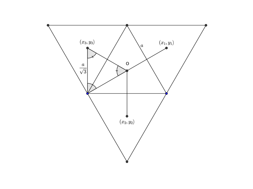
Figure 1: The construction to show the idea behind the approximation of the LB operator with the dual graph method.

The Taylor approximation to second order in $a$ around $O$ for a function $f$ evaluated at the points $\{(x_{i},y_{i})\}_{i=1,2,3}$ reads:

$$\begin{gathered}\forall i=1,2,3\;\;\;\;f(x_{i},y_{i})=f(0,0)+(x_{i},y_{i})\cdot\nabla f(0,0)+\\ +\frac{1}{2}\;[\partial_{x}^{2}f(0,0)x_{i}^{2}+\partial_{y}^{2}f(0,0)y_{i}^{2}+2\partial_{x}\partial_{y}f(0,0)x_{i}y_{i}]+o(a^{3}).\\ \end{gathered}$$ (15)

Then substituting the coordinates of the points:

$$\begin{gathered}(x_{1},y_{1})=\frac{a}{\sqrt{3}}(\frac{\sqrt{3}}{2},\frac{1}{2}),\\ (x_{2},y_{2})=\frac{a}{\sqrt{3}}(0,-1),\\ (x_{3},y_{3})=\frac{a}{\sqrt{3}}(-\frac{\sqrt{3}}{2},\frac{1}{2}),\end{gathered}$$ (16)

and summing the three Equations (15), one obtains:

$$\scriptstyle f(x_{1},y_{1})+f(x_{2},y_{2})+f(x_{3},y_{3})-3f(0,0)=\frac{1}{4}a^{2}\triangle f(0,0)+o(a^{3}),$$ (17)

implying

$$\scriptstyle\triangle f(0,0)=\frac{1}{a^{2}}\;4\;[f(x_{1},y_{1})+f(x_{2},y_{2})+f(x_{3},y_{3})-3f(0,0)]+o(a).$$ (18)

A similar relation holds for the center of each triangle of the simplicial manifold, so the LB operator is approximated through a matrix acting on a vector space of dimension equal to the number of triangles (the space of the possible values of the function in the centers):

$$-\triangle\leftrightarrow L\;=\;3\cdot\mathds{1}-A,$$ (19)

where $A$ is the adjacency matrix, whose entry $A_{ij}$ is $1$ if the triangles labeled with $i$ and $j$ are adjacent and $0$ otherwise. The factor $\frac{1}{a^{2}}$ is ignored since it is used as measure unit, while the factor $4$ is an overall scale factor, whose value will come in useful to compare the results with the new method that we will introduce in the next Section.

In higher dimensions, analogous calculations, that are possible only for regular (i.e., equilateral) simplices, lead us to approximate the Laplace-Betrami operator (forgetting for a while the overall constant) with the matrix:

$$-\triangle\rightarrow L\;=\;(d+1)\cdot\mathds{1}-A.$$ (20)

It is straightforward, though quite tedious, to prove that in generic dimension $d$ the overall numeric constant appearing in the analogous of Equation (18) equals $d^{2}$.

The matrix $L$ in Equation (20) shares many properties with the LB operator: it is symmetric and positive-semidefinite, with a unique eigenvector associated to the zero eigenvalue, the uniform function. Moreover, $L$ is sparse (most of its entries are $0$), thus making it possible to numerically calculate its spectrum using specifically optimized algorithms.

III Introduction to Finite Element Methods for spectral analysis

As apparent from the discussion in the previous section, one reason that drove us to introduce an alternative method to approximate the LB spectrum is that a faithful correspondence between the spectrum of the Laplace matrix of the graph dual to a triangulation and its exact Laplace-Beltrami spectrum requires, at least, the simplices to be regular, which is not the case for full CDT triangulations, where generic values of the parameter $\Delta$ encode the asymmetry between spacelike and timelike links in the Euclidean space.

Moreover, for the method that we are going to introduce, it is always possible to set up an iterative procedure (Appendix A.3) whose convergence to the exact spectrum of the LB operator is guaranteed by standard theoretical results in literature.
In the following, we outline the basic ideas the Finite Element Method relies upon, leaving the technical details of our application to CDT to Appendix A.

Finite Element Methods (FEM) are a family of approximation techniques for the solution of partial derivative equations that is widely studied and applied in many fields where complex modeling is necessary fem_allairebook ; fem_hughesbook ; fem_strangbook ; fem_taylorbook ; fem_babuska . Complex objects are decomposed into simpler smaller parts to reduce the number of degrees of freedom to a finite one, which is far easier to be dealt with.
The application of FEM in the context of spectral analysis of manifolds relies upon a weak formulation of the Laplace-Beltrami eigenproblem, which, on a (simplicial) manifold $\mathcal{M}$ without boundary takes the form:

$$-\triangle f(\mathbf{x})=\lambda f(\mathbf{x}).$$ (21)

By multiplying both sides of this equation with an arbitrary test function $\phi$, and integrating over the whole manifold, we obtain:

$$\int_{\mathcal{M}}\!d^{d}x\;\nabla\phi(\mathbf{x})\nabla f(\mathbf{x})=\lambda\int_{\mathcal{M}}\!d^{d}x\;\phi(\mathbf{x})f(\mathbf{x}),$$ (22)

where a step of integration by parts has also been performed.

This second form, where $f$ is assumed to be a reasonable object (like a Sobolev function or a distribution), is equivalent to the one in Equation (21). Nonetheless, it is useful to see the problem in this form because its natural environment of definition is wider. The usual environment for these kinds of problems is the Sobolev space $H^{1}(\mathcal{M})$, the space of $L^{2}$ scalar functions that admit weak first derivatives, as it is a set of quite regular functions in which it can be proved that solutions exist for the problem. In the following, we refer to the spectrum of the LB operator on the class of $H^{1}(\mathcal{M})$ scalar functions as the exact LB spectrum.

FEM consists in solving a problem similar to the one shown in Equation (22) in a sequence $\{\mathcal{V}_{r}\}_{r=0}^{\infty}$ of particular finite-dimensional subspaces of $H^{1}$ with increasing dimension $\mathcal{V}_{r}\to H^{1}$, whose eigenvectors $f_{n}^{(r)}$ and eigenvalues $\lambda_{n}^{(r)}$ converge to the exact LB eigenvectors and eigenvalues of the infinite-dimensional problem (22) in $H^{1}$.

In these finite-dimensional subspaces, as outlined in Section A.1, the problem consists in nothing but an eigenproblem of a finite-dimensional matrix, whose entries are calculated in Section A.2.
Because of the (quite natural) choices we make to define our sequence of subspaces for our simplicial manifolds, this progression can be seen as a series of subsequent refinements of the starting triangulation: each step consists in subdividing every simplex of the triangulation into smaller ones, while preserving a simplicial manifold structure. For details, see Section A.3.

IV Comparison between FEM and dual graph methods on test geometries

Before delving into the application of FEM to real CDT cases, it is useful to investigate its behaviour in some simple exemplar situations. This, besides providing us with some checks on the expected convergence of the method to the exact LB spectrum of the manifolds, allows also a useful comparison between the FEM and the dual graph method.

We proceed as follows:

1. we check the convergence of the method in some cases where the exact LB spectrum on the manifold is known analytically;

2. we consider two dimensional simplicial manifolds made of regular simplices, where a refinement procedure is available also for the dual graph method, in order to show how both approaches converge to the exact LB spectrum;

3. we notice that our results imply that the standard (not refined) application of both methods yield estimates of the eigenvalues which can be significantly at variance with the ones of the exact LB spectrum, while the refined version (generally unavailable to the dual graph method) shows a good convergence behavior;

4. finally, by means of a toy model, we provide a reason why the eigenvalues obtained with the dual graph method typically undershoot the ones of the exact LB spectrum.

IV.1 Convergence of the method for manifolds with known spectrum

First of all, we check the convergence of FEM to the exact LB spectrum for some manifolds that can be seen as simplicial manifolds and whose spectrum is known: flat toruses. Indeed, they are nothing but flat parallelepipeds with properly identified boundaries, and it is apparent that they can be covered with simplices, though not with regular ones, except for some specific ratios of their “sides”.

For a generic $d$ dimensional smooth torus, with lengths $\{L_{\mu}\}_{\mu=1}^{d}$, the LB spectrum reads:

$$\mathcal{S}_{d}[L_{\mu}]\equiv\Big{\{}4\pi^{2}\sum\limits_{\mu=1}^{d}\Big{(}\frac{n_{\mu}}{L_{\mu}}\Big{)}^{2}\Big{|}n_{\mu}\in\mathbb{Z},\mu=1,\dots,d\Big{\}},$$ (23)

where we order the eigenvalues in a non-decreasing fashion, and consider degenerate eigenvalues as distinct elements.

Figure 2 displays the eigenvalues obtained with FEM at four subsequent refinement levels (see Section A.3) in comparison with the exact LB eigenvalues from Equation (23), for a two-dimensional flat torus with arbitrarily chosen sides $L_{x}=3.1$ and $L_{y}=1.2$. As expected from a theoretical point of view (see Section A.1), the FEM eigenvalues converge to the exact LB spectrum from above, and are more accurate in the the lower part of the spectrum (i.e., for larger scale modes).

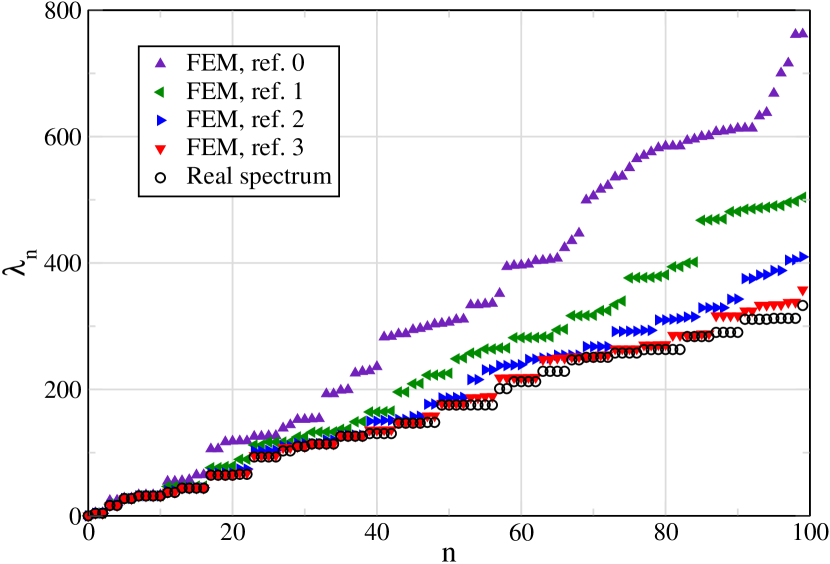
Figure 2: Convergence of the first $100$ eigenvalues, obtained through FEM, to exact spectrum for a 2D flat torus with spatial sizes $L_{x}=3.1$ and $L_{y}=1.2$. In figure, we show a sufficient number of refinement levels to reach convergence to the real spectrum within 1% in its low part.

The same behavior is observed for a flat torus in three dimensions; the only difference found is in the computation time needed to achieve the same precision, that becomes greater the higher the dimension, because convergence rate depends on the maximal diameter $h$ among the simplices fem_hughesbook ; fem_strangbook , while computation time depends, given our choices, on the number of vertices, which, for the same decrease in $h$, grows faster in higher dimension. Results obtained for a 3D flat torus with $L_{x}=1.4$, $L_{y}=1.9$, $L_{z}=1.2$ are shown in Figure 3. A similar behavior is observed also for higher-dimensional toruses, which however don’t add interesting information to what we have already shown.

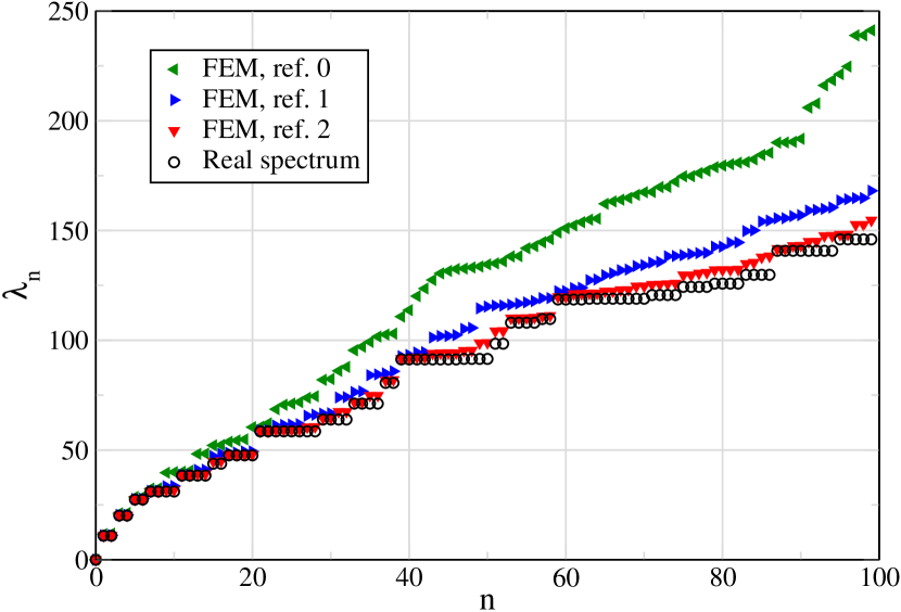
Figure 3: Convergence of the first 100 eigenvalues obtained via FEM to the exact spectrum for a 3D flat torus with spatial dimensions $L_{x}=1.4$, $L_{y}=1.9$, $L_{z}=1.2$.

IV.2 Focus on dimension two: refinement for the dual graph method and convergence of FEM for irregular simplicial manifolds

Here we investigate what happens with two-dimensional toruses which can be covered by equilateral triangles (those with $L_{y}=\sqrt{3}L_{x}$), as they allow a direct comparison between FEM and the dual graph method. Notice that, for such a comparison, the overall numeric factor in Equation (18) ($4$, in two dimensions) becomes relevant.

As anticipated above, a particularity of dimension two is that we can think of a refinement procedure of the simplicial manifold that allows to iterate the dual graph method: it consists in dividing each equilateral triangle into four new ones by connecting with three new links the middle points of the sides of each triangle. Figure 4 shows the spectra in the case of a two-dimensional flat torus made of $20$ rows of $20$ equilateral triangles of unit side ($L_{x}=10$) with properly identified boundaries. At increasing refinement level, besides the expected convergence of the FEM spectrum to the exact LB spectrum (from above), we observe also a convergence of the dual graph spectrum from below, even if we do not have a well-settled theory ensuring this behavior (unlike in the FEM case). The interpretation of this behavior will turn out to be fundamental (see Section IV.4).

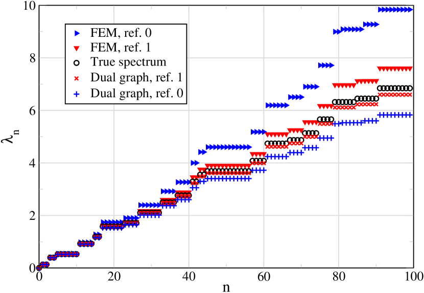
Figure 4: Convergence of the first $100$ eigenvalues, obtained via FEM and dual graph method, for a 2D flat torus made of $20$ rows of $20$ equilateral triangles with unit side, with appropriate identification. Dual graph eigenvalues have been multiplied by $4$ for comparison with FEM ones, as explained in the text.

The dual graph method behaves in the same way as in the previous example also on a less regular object, like a typical two-dimensional CDT configuration, whose exact LB spectrum cannot be computed by analytical means. This helps us check the convergence properties of FEM even on such an irregular object: in Figure 5, indeed, we can compare the two methods as they progressively reach an agreement, following two opposite trends (FEM from above and dual graph from below), on what can be guessed to be the exact LB spectrum on this real-life CDT object. Not very surprisingly, computation times are worse than for more regular geometries.

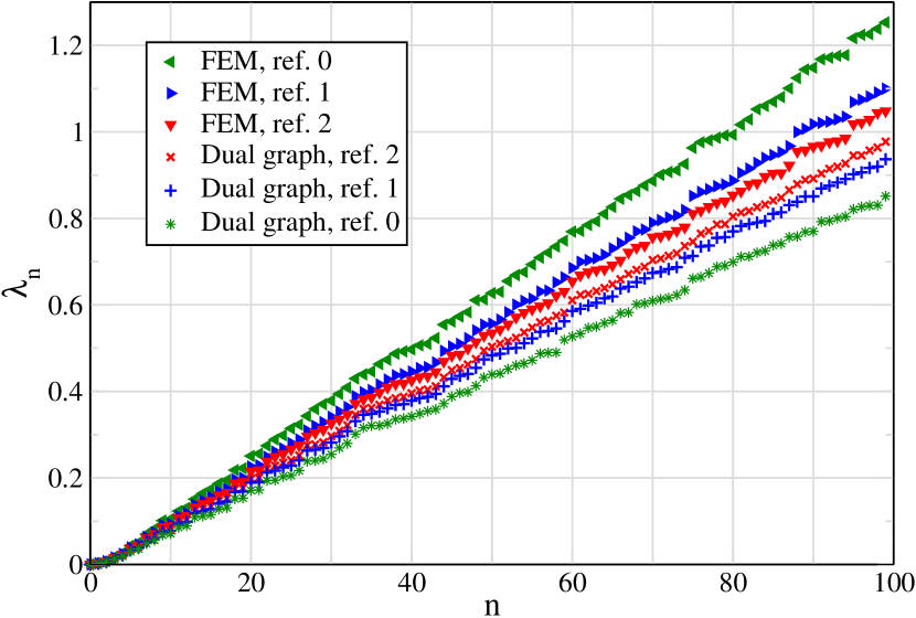
Figure 5: Convergence of the first $100$ eigenvalues of LB operator, discretized by means of the two methods, on a random test CDT configuration in two dimensions. The configuration has total volume $2602$ and $1301$ vertices. Dual graph eigenvalues have been multiplied by a prefactor $4$ for comparison with FEM ones, as explained in the text.

IV.3 General inaccuracy of the dual graph method in the case of no refinement steps

Besides being a check for the convergence of FEM, the two examples of the previous section testify the fact that the spectrum of the Laplace matrix of the original unrefined dual graph quantitatively differs in a non-negligible way from the exact LB spectrum: indeed, we stress again that, in more than two dimensions, no refinement for the dual graph is available, so the situation one faces is the same as in Figure 5 but with only the $0$th refinement (the original triangulation). An example of this is shown in Figure 6, depicting the spectrum obtained with the two methods on a spatial slice of a 4D CDT configuration coming from a point in $C_{dS}$ phase (using $9$ as the overall factor for the dual graph method).

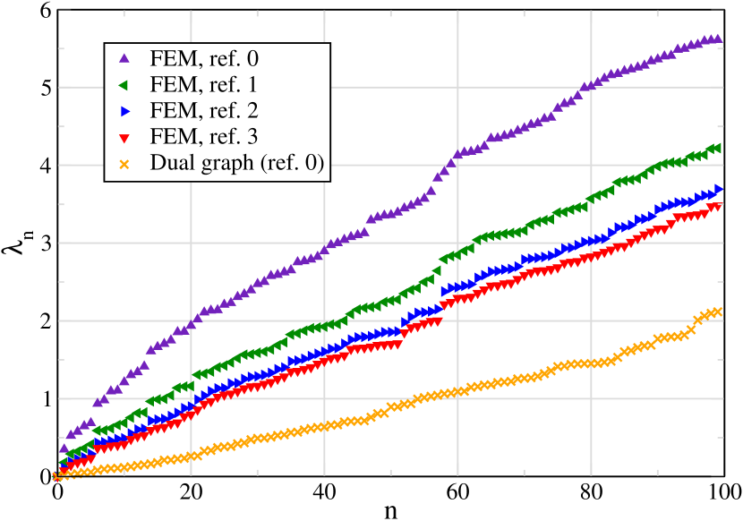
Figure 6: Convergence of the first $100$ eigenvalues of LB operator, obtained by means of the two methods, on a spatial slice (with $V_{S}=2631$) of a random test CDT configuration in four dimensions. Dual graph eigenvalues have been multiplied by $9$ for comparison with FEM ones, as explained in the text.

What we show in the next section is that the difference of the dual graph spectrum from the exact one can be so large that it could lead to misrepresent even some important (large scale) qualitative features of the simplicial manifold.

IV.4 Issues of the dual graph method: discussion and a toy model

In order to understand the reasons for the quantitative discrepancies shown in the previous section between the (unrefined) dual graph spectrum and the exact LB spectrum, it is important to establish why the first seems to systematically underestimate the second, as apparent from Figures 4, 5 and 6.

Regarding this observation, we have a tentative explanation, which we think may prove to be quite compelling after we show a simple toy model serving as a worst-case scenario.

As explained in Section II.1, if we consider a diffusion process on a manifold, the eigenvalues of the LB operators are associated with the typical time rates of the diffusion modes and to the typical length scales of the manifold. When we build the dual graph associated with a simplicial manifold, we lose part of the metrical information that is relevant to a diffusion process on that object, which is not merely made of the adjacency relations between simplices. A diffusion process on a simplicial manifold takes place in the whole physical space of which it is constituted, and not only along the segments connecting the centers of adjacent simplices: the main consequence of this fact is that in the dual graph case the distance between two centers “perceived” by a diffusing particle is incorrectly represented by the adjacency matrix, as if the particle was constrained to diffuse along the segments joining the centers instead of going from one point to another along the shortest path (i.e., a geodesic of the simplicial manifold). This happens because we have lost memory of the metric al information (and, in some sense, also of the topology, as we will show in the toy model) of everything that is not the centers, the edges between them and the angles between the edges (which the correspondence to the LB operator relies upon). Therefore, we claim that all typical length scales are overestimated and the error depends on how badly the geodesics are approximated by broken lines passing through the centers, thus resulting in the underestimation of the eigenvalues they are associated with; this idea is depicted in Figure 7.

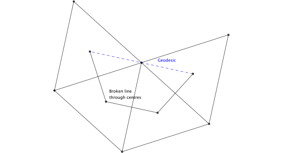
Figure 7: An example of the physical distance between two centers being overestimated by the path through centers connecting them.

In light of these considerations, the observed convergence from below of the eigenvalues in two dimensions, where a meaningful refinement procedure is available, can be naturally understood as the fact that shortest paths connecting centers in the dual graphs approach more and more, at increasing refinement level, the true geodesics of the simplicial manifold.

The information we are losing by neglecting the flat interior of simplices does not have to be taken into account when we set up simulations using the Einstein-Hilbert action in the coordinate-free Regge formalism, because that requires only the total volume and the total curvature, information that can be represented in terms of combinatorial observables. However, in order to describe the geometry of a simplicial manifold in terms of local observables (like the propagation or diffusion of test fields) one has to take into consideration the whole geometrical structure, including that information.

An objection to the necessity of the FEM representation as a substitute to the dual graphs one could be that, since the interior of a simplex in the original triangulation is flat, and its sizes are comparable with the lattice spacing, the results expected using dual graph techniques (including non-spectral ones) would have no substantial effect on large scale observables, whose correlation lengths are assumed to be much larger than the lattice spacing, therefore making dual graph results inaccurate just only for small scales features which would be discarded anyway. However, even if this argument may work sometimes (e.g., for hypercubic lattices representing flat spaces), it doesn’t hold in this case. The key fact is that the length scales provided by the dual graph method do not correspond to actual physical scales of the manifold in a clear way, and the relation depends on the geometric properties of the manifold under analysis, as the geodesic overestimation resulting from the dual graph representation can severely and differently impact the observables, even at large scales. This geodesics overestimation can be responsible for arbitrarily poor estimates when the total volume goes to infinity, being it possible to make the dual graph method detect the biggest length scale as going to infinity while it is actually staying finite. This would result in the dual graph method yielding a vanishing spectral gap in the infinite volume limit, with the real LB spectrum actually having a lasting non-zero gap.

Indeed, it is not hard to realize that the worst case of distance overestimation happens in the neighborhood of $(d-2)$-simplices with high coordination numbers (i.e., those associated with a high local negative curvature): the geodesic distance between the centers of two “opposite” $d$-simplices sharing a $(d-2)$-simplex with many $d$-simplices surrounding it, that is roughly the diameter of the $d$-simplices, is very badly estimated by a broken line passing through the centers, that is a very long (half) loop around the $(d-2)$-simplex. This observation inspires the construction of a simple 2D model that we will now discuss: we consider an arbitrary number of triangles all sharing the same vertex, with each of the links coordinated to it in common between two of them; then, in order to make the manifold boundaryless, we take a second identical “sheet” of triangles forcing each triangle of the first sheet to share the third side with the third side of the corresponding triangle of the second sheet. In this setting, we show how by increasing the total volume the FEM correctly detects an almost constant non-vanishing spectral gap, while the dual graph method yields a vanishing one, since it represents this object essentially as a discretization of $S^{1}\times\{0,1\}$.

Because of the highly pathological geometry, it is not easy to push the FEM to convergence, that in this particular case we see to be slower for lower-order eigenvalues than for higher-order ones: within reasonable computation times we could achieve stable estimates (within 1%) of the orders between, say, $n=10$ and $n=20$, but not of the spectral gap. Given that we have a specific interpretation of the meaning of the spectral gap, we prefer, anyway, to focus on it rather than on other orders: even without explicit achievement of convergence, indeed, in Figure 8 we can see how when the volume increases (we use as progression $V=100,200,400,800,1600$) the spectral gap seen at each refinement step by the FEM is almost constant, with values that become more and more similar at increasing volume as can be seen in the inset plot. The exact LB spectral gap, i.e., the one at infinite refinement level, gets the same non-zero value independently on the volume. This is expected, the diffusion rate being more related on the finite manifold diameter (the maximum of minima among path lengths) than on its volume.

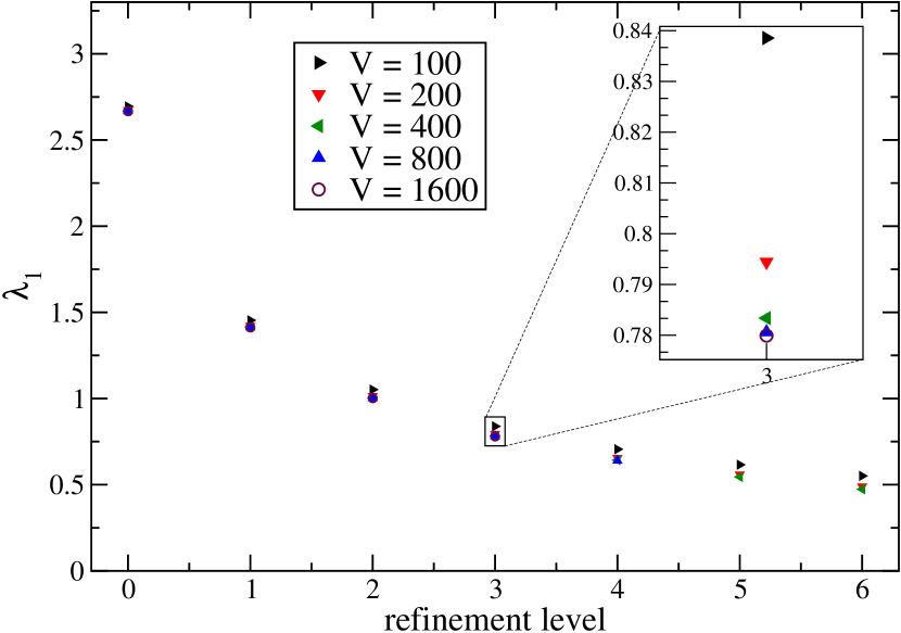
Figure 8: Estimate for the spectral gap as a function of the refinement step for the toy model at various volumes. For a given refinement step, the estimates for the spectral gap are very similar for big volumes, thus the exact value can be expected to be essentially the same too.

The dual graph method, instead, detects a spectral gap quadratically decaying to zero for the same volume progression as above, as one can predict by considering the aforementioned $S^{1}$ structure of the dual graph of this simplicial manifold. This is shown in Figure 9.

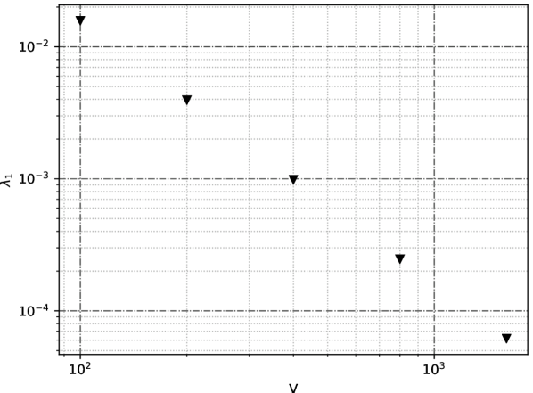
Figure 9: Spectral gap detected via dual graph method for the toy model at various volumes. The value vanishes quadratically as expected. Both scales are logarithmic.

We have seen, then, that the dual graph method gives estimates that not only quantitatively differ from the exact LB spectrum on the manifold (with the consequent different estimates for related spectral observables, as we show below) but can also fail to reveal some important qualitative geometrical features as a finite diameter for infinite volume, a situation that might even result not to be irrelevant for CDT, where infinite volume represents the thermodynamic limit, even if the randomness of geometry would probably prevent such extreme situations from happening.

V Numerical results

Having explained our motivations for applying FEM to the study of the LB spectrum on simplicial manifolds, here we show it in action on CDT, where we obtain results that significantly differ from analogous ones obtained by using the dual graph method. In particular, for the sake of comparison, we considered the large-scale dimension of spatial slices in $C_{dS}$ phase and the critical index of the $C_{b}$-$C_{dS}$ transition along the line $k_{0}=0.75$, which were already investigated in lbrunning using dual graph methods.

Both of these results involve the spectral analysis of spatial slice submanifolds, for which the thermodynamic limit is assumed to coincide with the behavior at large spatial volume $V_{S}$: the underlying assumption is that the overall volume fixing, if large enough (in all of our simulations $V_{S,tot}=80k$), does not significantly affect the features of spatial slices. This assumption should be verified by checking the stability of the results under the increase of the total spatial volume, a computationally demanding operation that we postpone to future works, our main aim now being to show the potential of these methods. Furthermore, since computational costs for even the low part of the FEM spectrum grow rapidly when the refinement level increases, we need to resort to an extrapolation at infinite refinement level, as we discuss next.

Summarizing, the following three limiting procedures should be performed in this specific order:

• for each simplicial manifold $\mathcal{M}$, extrapolation of the individual FEM eigenvalues to “infinite refinement level” $\lambda_{n}^{(r)}[\mathcal{M}]\xrightarrow{r\to\infty}\lambda_{n}^{(\infty)}[\mathcal{M}]$, in order to obtain an accurate enough approximation of the spectrum of the exact LB differential operator on $\mathcal{M}$;

• for each ensemble of configurations at specific values of the parameters, one should first perform an average of the eigenvalues at each specific order $n$ and then take the thermodynamic limit (i.e., infinite volumes in lattice units) ${\langle\lambda_{n}\rangle}_{V}\equiv\frac{1}{\lvert\mathcal{C}_{V}\rvert}\sum_{\mathcal{M}\in\mathcal{C}_{V}}\lambda_{n}^{(\infty)}[\mathcal{M}]\xrightarrow{V\to\infty}{\langle\lambda_{n}\rangle}_{\infty}$ by considering the spectra of ensembles $\mathcal{C}_{V}$ with increasing volumes;

• study the critical scaling of the twice-extrapolated eigenvalues ${\langle\lambda_{n}\rangle}_{\infty}{(k_{0},\Delta)}$ observed as the phase transition is approached.

V.1 Extrapolation to infinite refinement

Both the results we are going to show are relative to the LB spectrum on the spatial slices, so we have to deal with great variability in the volumes: first of all, then, we group the slices in a proper number of volume bins (excluding too small ones). This is anyway necessary, regardless of the extrapolation step, in order to study the thermodynamic limit; indeed, this was done also when the dual graph method was used (see lbrunning ). Then, for each fixed refinement level, we average the eigenvalues of each fixed order $n$ of the slices in each volume bin, using the standard deviation of the mean as a measure of uncertainty; finally, we extrapolate the value for infinite refinement level for each order and bin, that we read as a reasonable estimate of the average in that volume bin of the exact LB eigenvalues of that order.

The functional form we use for our extrapolation is

$$\lambda_{n}^{(r)}=\lambda_{n}^{(\infty)}+A_{n}e^{-r/B_{n}},$$ (24)

where r is the refinement level, $A_{n}$ and $B_{n}$ two parameters that depend on the order of the eigenvalue and on the volume bin and $\lambda_{n}^{(\infty)}$ the extrapolated value. The reason why we use this form is that the most relevant parameter for the convergence of FEM is the maximal diameter $h$ among the simplices of the triangulation: the convergence to the exact LB eigenvalues fem_hughesbook ; fem_strangbook , given that the simplices are not too pathological (e.g., having very acute angles), can actually be faster than a power of $h$. Assuming our “average” convergence to happen exactly according to a power of $h$, from the fact that in our case $h$ is halved at each refinement step, we obtain:

$$\lambda_{n}^{(r)}=\lambda_{n}^{(\infty)}+h^{k}=\lambda_{n}^{(\infty)}+h_{0}2^{-rk},$$ (25)

that can be rewritten in the form of Equation (24). We show below that our data are in good agreement with this picture.

V.2 Large-scale spectral dimension of spatial slices in $C_{dS}$ phase

In previous studies with dual graphs lbstruct ; lbrunning ; lbpos19 , the large-scale effective dimension of the spatial slices in phase $C_{dS}$ seemed to be almost independent of the point in the $C_{dS}$ phase, and compatible regardless of the definition of dimension: the “diffusive” one and the one based on “energy-levels”, both introduced in Section II.

It was reasonable to choose to analyze two of the phase space points in which the known estimates were obtained, that is, $(k_{0},\Delta)=(2.2,0.6)$ and $(k_{0},\Delta)=(0.75,0.7)$. The maximum number of refinements levels we could analyze with the resources available was $\bar{r}=3$ (besides the starting triangulation, labeled as $r=0$). In both cases, the bins we used were of equal volume extent and were chosen in such a way that the slices were, more or less, equally distributed; moreover, we excluded from the analysis slices with volumes $V_{S}<500$, for which finite volume effects could be significant. The best-fit of the extrapolations performed for each volume bin, according to the functional form in Equation (24), shows, in almost every case, a good agreement between data and our chosen heuristic form, with $\chi^{2}$ ranging between $0.5$ and $3.5$ (one degree of freedom). Then, for both of the two points we performed two different best-fit procedures to find an estimate of the large-scale spectral dimension. The first form considered was:

$$\langle\lambda_{n}\rangle=A_{n}V_{S}^{-2/d_{EFF}},$$ (26)

for a global fit using the first ten eigenvalue orders with $d_{EFF}$ and $\{A_{n}\}_{n=1}^{10}$ used as free parameters ($d_{EFF}$ in common for every order $n$).
The second form considered was:

$$\langle\lambda_{n}\rangle=(n/V_{S})^{2/d_{EFF}},$$ (27)

that, as the previous one, can be obtained from Equation (14), again for the first ten orders, where the effective dimension $d_{EFF}$ is the only free parameter and corresponds to the dimension of the simplicial manifold at the largest scale (lowest part of the spectrum).

At each point, we also performed the same two procedures by using the values that could be extrapolated from the first two refinements only, in order to have a further indication of the goodness of our heuristic extrapolation method by confronting the obtained results with ($\bar{r}=3$) and without ($\bar{r}=2$) using the third refinement. We saw general compatibility of the extrapolated values of $\langle\lambda_{n}\rangle$, with a slight systematic overestimation in the case without refinement $3$ with respect to the other.

Fit results for the point $(k_{0},\Delta)=(2.2,0.6)$ are shown in Table 1, where the functional forms in Equations (26) and (27) and with refinements up to $\bar{r}=2$ and $\bar{r}=3$ have been considered independently. Figure 10 represents extrapolated eigenvalues and best-fit with the function in Equation (26) including the third refinement ($\bar{r}=3$), while Figure 11 shows the same in the case of a fit with the function in Equation (27). The compatibility between the estimates with ($\bar{r}=3$) and without ($\bar{r}=2$) using the third refinement is not exceptional but neither terrible, and, in general, the first estimate should be preferred, of course, as it involves a broader dataset.

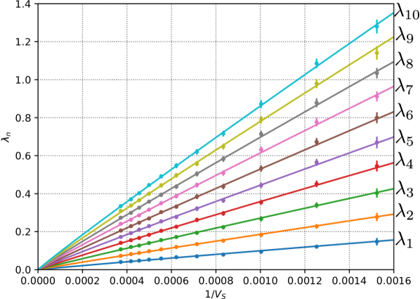
Figure 10: Extrapolated first ten orders of eigenvalues vs $1/V_{S}$ for big enough slices ($V_{S}>500$), with best-fit curves according to Equation (26) (common $d_{EFF}$). Phase space point $k_{0}=2.2,\Delta=0.6$, volume fixing $V_{S,tot}=80k$.

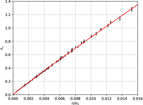
Figure 11: Same as in Figure 10, but using Equation (27) as fitting function, and data collapsed by using $n/V_{S}$ as independent variable.

Fit function	$d_{EFF}$ [$\chi^{2}/dof$] Eq. (26)	$d_{EFF}$ [$\chi^{2}/dof$] Eq. (27)
$\bar{r}=2$	$2.129(34)$ [$4/99$]	$2.14(3)$ [$5/108$]
$\bar{r}=3$	$2.084(16)$ [$15/99$]	$2.091(12)$ [$16/108$]

Table 1: Fit results of the functional forms in Equations (26) and (27) for the FEM extrapolations of the first ten orders of eigenvalues (see Figures 10 and 11) for spatial slices of configurations at the point $(k_{0},\Delta)=(2.2,0.6)$.

In general, as it can be seen, data well fit a large-scale finite and fixed effective dimension, and the two different best-fit procedures return compatible estimates for the effective dimension, but this dimension significantly differs from the previously known value of about $1.6$ found in lbstruct . We choose as our conservative estimate the average of the two most reliable estimates ($\bar{r}=3$): $d_{EFF}=2.088(18)$ (with the semidispersion as error).

As for the point $(k_{0},\Delta)=(0.75,0.7)$, we performed the same kind of analysis, obtaining the results shown in Table 2. The plots for this point of the phase diagram are qualitatively similar to 10 and 11, and will not be shown. As before, the results are somewhat compatible, and the estimates with $\bar{r}=3$ are preferred. Again, we see the expected fixed and finite-dimensional behavior, and the estimated dimension significantly differs from that of about $1.6$ found in lbrunning : our conservative estimate, indeed is $d_{EFF}=2.202(16)$.

Fit function	$d_{EFF}$ [$\chi^{2}/dof$] Eq. (26)	$d_{EFF}$ [$\chi^{2}/dof$] Eq. (27)
$\bar{r}=2$	$2.28(3)$ [$7/99$]	$2.25(2)$ [$10/108$]
$\bar{r}=3$	$2.216(15)$ [$23/99$]	$2.187(11)$ [$34/108$]

Table 2: Fit results of the functional forms in Equations (26) and (27) for the extrapolations of the first ten orders of eigenvalues for spatial slices of configurations at the point $(k_{0},\Delta)=(0.75,0.7)$.

Interestingly, the two final estimates, besides being incompatible with the ones previously known in literature, appear to be quite different for the two phase space points, while up to now it has been believed that this dimension is almost constant across the $C_{dS}$ phase. This may be worthy of further inquiry as it might turn out to be significant, for example, for the study of the RG flow properties in that phase.

V.3 Critical index of $C_{b}$-$C_{dS}$ transition

The most interesting result from lbrunning is the analysis of the critical behavior of the low spectrum of $B$-type slices in phase $C_{b}$ while approaching the $C_{b}$-$C_{dS}$ transition along two lines of constant $k_{0}$. Here we compare the results from lbrunning , obtained using dual graph methods, with the application of FEM to the same configurations, in particular, checking the value of the critical index $\nu$ in the shifted power law:

$$\langle\lambda_{n}\rangle_{\infty}=A_{n}(\Delta_{crit}-\Delta)^{2\nu}.$$ (28)

We analyzed some points along the line $k_{0}=0.75$ only, and considered the critical scaling of the first ten orders of eigenvalues at the same time. First, we had to extrapolate to infinite refinement level, which we did in the same way as described above using Equation (24) on data coming from refinements $0$ up to $\bar{r}=3$, and then to the thermodynamic limit ($V_{S}\to\infty$) for each order. For this second procedure, not having precise expectations on the large-scale behavior but the fact that each order should not approach zero, we followed lbrunning and used the simplest form compatible with data, that is, a quadratic polynomial in $1/V_{S}$:

$$\langle\lambda_{n}\rangle=\langle\lambda_{n}\rangle_{\infty}+\frac{A_{n}}{V_{S}}+\frac{B_{n}}{V_{S}^{2}}.$$ (29)

Figure 12: First ten eigenvalue orders of spatial slices (with $V_{S}>500$) vs $1/V_{S}$, with extrapolation to the thermodynamic limit ($V_{S}\rightarrow\infty$) in $C_{b}$ phase. Phase space point $(k_{0},\Delta)=(0.75,0.7)$, total spatial volume $V_{S,tot}=80k$.

For every phase space point taken into account, both procedures gave satisfactory results in terms of the agreement between data and model: for the infinite refinement extrapolations, the chi-squared was $2$ in the worst case (with $1$ dof), while the thermodynamic limit extrapolations always yielded $\chi^{2}/dof<1$. For illustration purposes, Figure 12 displays the extrapolation to the thermodynamic limit for the first ten eigenvalue orders in the phase space point $k_{0}=0.75,\Delta=0.575$.

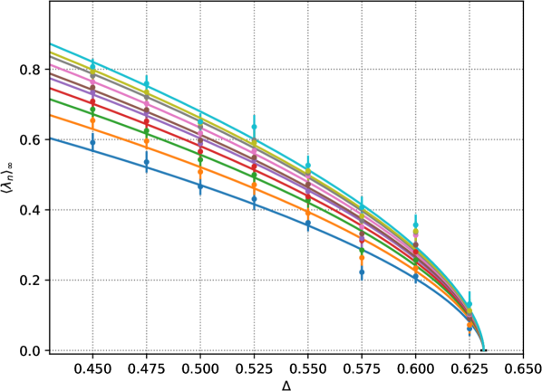
Figure 13: Critical behavior of the first ten eigenvalue orders along the line at fixed $k_{0}=0.75$ and varying $\Delta$, with best-fit curves of the form shown in Equation (28) with common $\nu$ and $\Delta_{crit}$. Curves of increasing eigenvalue order are shown from below to above in the plot.

We then analyzed the first ten eigenvalue orders by fitting our data with Equation (28), forcing the critical index $\nu$ and the critical point $\Delta_{crit}$ to be the same for every order. We used data coming from eight phase space points with $\Delta$ ranging from $0.45$ to $0.625$: we chose not to go too deep inside $C_{b}$ phase because of the influence of the expected sub-dominant terms of the critical scaling and excluded them by checking the stability of our estimate of $\nu$ under the removal of the points with lower $\Delta$ parameter. We obtained, as best-fit parameters $\nu=0.293(10)$ and $\Delta_{crit}=0.6316(15)$, with $\chi^{2}\approx 67$ ($68$ dof); our data and best-fit curves are displayed in Figure 13.

It is apparent that data (from a bigger dataset) are still compatible with the critical scaling found in lbrunning , but, while the estimated location of the transition line agrees with the previous findings, the value we found for the critical index significantly differs from the previous estimate. We remark that a difference like this may be of great importance if critical indexes of different observables have to be compared to find a physical continuum limit in the phase diagram.

VI Summary and Conclusions

In this work, we have reviewed some concepts about spectral analysis on simplicial manifolds using the dual graph representation, discussing its domain of definition (triangulations with equilateral simplices, which can be mapped to undirected graphs), and its limitations, it being an approximation to the Laplace-Beltrami operator (in the sense recalled in Section II.3) acting on the whole infinite-dimensional $H^{1}$ space on the simplicial manifold.

In order to extend the use of the spectral observables beyond this domain, we introduced the Finite Element Method formalism and its application to the solution of the LB eigenproblem (Section III, with details left to Appendix A). The two representations, dual graph and FEM, were compared on a series of test geometries in Section IV, showing that, while the dual graph method and FEM display convergence to the same spectrum when a refinement procedure is applicable in both cases (that is, only for two-dimensional equilateral triangulations), when this procedure is not available, the results provided by the two methods differ in a non-negligible way.

We tried to explain this disagreement between the dual graph and FEM representation by identifying the main reasons in the phenomenon of geodesics overestimation, and in the lack of a general procedure ensuring convergence to the exact spectrum of the LB differential operator(which is linked to the geodesics of the simplicial manifold in the way outlined in Section II.1); this spectrum is instead obtained as the limit of the FEM procedure at infinite refinement level, “curing” the geodesic overestimation. We showed that this overestimation can affect also the large scale behavior of observables, in particular when large loops in the dual graph are involved (a loop being made of many $d$-simplices encircling around a $d-2$-simplex), as discussed using an illustrative toy model in Section IV.4.

Finally, in Section V, we compared some earlier dual graph spectral results on CDT spatial slices with the results of the application of the FEM approach. We have shown that the FEM effective dimension observed on spatial slices in two points of the phase diagram in the $C_{dS}$ phase region is significantly different from the one observed using dual graph techniques, and that while the dimensions for the two points seemed to be compatible in the dual graph case, with $d_{EFF}\simeq 1.6$, they are detected as incompatible in the FEM case. We have also investigated again, but using FEM techniques, the critical behavior near the $C_{b}$-$C_{dS}$ transition along a line in the $C_{b}$ phase at $k_{0}=0.75$ as in lbrunning : while our estimation of the the critical parameter $\Delta_{crit}$ is compatible with the earlier result, we found that the critical index significantly differs from the previous estimate.

We regard this last result as the most relevant of ours, as it points out that the use of the dual graph method might be questioned in some cases. Observing different critical indices in the approach to a phase transition line, indeed, implies that the length scales found by using the two methods cannot be simultaneously compared with other length scales coming from different observables to look for a continuum limit.

While the FEM, extrapolated at high refinement levels, gives access to large scale properties of the full simplicial manifold, one big advantage of the dual graph approach is its relatively low computational cost. It might well be that in approaching a CDT continuum limit the two methods would show an agreement, or that their disagreement could be corrected by studying the scaling of some dimensionless parameters that may connect the length scales provided by the two methods. Nevertheless, we believe our warning should be taken into account by future studies, and the FEM should remain as a useful tool for CDT investigations.

The broadness of the Finite Element Method framework allows for extensions and variations which we had no time and resources to consider in this work. For example, the freedom in the choice of the refinement procedure can make for faster convergence, by using higher-order basis functions, or a mix of these with mesh refinements, or other types of FEM representations. Furthermore, in this work, we have only considered the application of FEM to the LB eigenproblem, but the formalism is powerful enough to undertake more general tasks, like a properly defined representation of the introduction of new coupling terms in the action, both gravitational ($f(R)$ extensions) and with matter and gauge fields (whose propagation properties would be unbiased by the geodesic overestimation of the dual graph representation), or the study of observables which have been limited in their definition by the attempts of embedding it in a dual graph structure, like the Wilson loop observable introduced in cdt_Wilson_loop . In general, having access to the true geodesics of the simplicial manifolds (or at least to an arbitrarily good approximation of them), can also be useful, for example, to build and describe light cone observables, which may have, in principle, interesting phenomenological implications.

We plan to discuss the more challenging task of applying FEM techniques to the LB eigenproblem of full four-dimensional CDT configurations in a future work, as the refinement procedure requires more computational resources at higher dimensions. Apart from the geodesic overestimation, for the analysis of four-dimensional CDT configuration there is also the problem that dual graph cannot faithfully represent the metrical properties of triangulations, but only their adjacency relations, since the Wick rotated spacelike and timelike links have not, in general, the same length (apart for $\Delta=0$), and we stress again that the Laplacian matrix of the dual graph has a clear relation with the LB operator only for equilateral triangulations. Therefore, the FEM formalism (or any other formalism taking into consideration the anisotropy in four-dimensional $4$-simplices) could be used instead, and this may have, for example, important effects on the form of the dimensional reduction pattern cdt_spectral_dim . We have also left out an analysis of the structure of FEM eigenvectors, which, together with the eigenvalues, contain complete information on the geometrical properties of the manifolds. A possible application of the eigenvectors is briefly discussed in the Appendix, where we define a Fourier transform of the local curvature observable, which can be useful, for example, to the construction of a smoothed curvature observable (by truncating contributions from eigenvector associated to eigenvalues above a threshold).

Appendix A Technical details of the application of FEM to CDT simplicial manifolds

In the following we explain in detail how we apply the FEM to our case of interest, the calculation of the LB eigenvalues on a simplicial manifold: in Section A.1 we show that each step of the method consists in solving the eigenproblem of a finite-dimensional, symmetric matrix; in Section A.2 we explain how we calculate the matrix elements and solve this problem for each step; in Section A.3 we outline the way we choose the sequence $\{\mathcal{V}_{r}\}_{r=0}^{\infty}$ of subspaces of $H^{1}$ we need for the application of the FEM, that in our case turns out to be a refinement procedure for our simplicial manifold.

A.1 LB eigenproblem in a FEM finite-dimensional subspace

As stated in Section III, in each step of the FEM the LB eigenproblem is reduced to the eigenproblem:

$$\int_{\mathcal{M}}\!d^{d}x\;\nabla\phi(\mathbf{x})\nabla f(\mathbf{x})=\lambda\int_{\mathcal{M}}\!d^{d}x\;\phi(\mathbf{x})f(\mathbf{x}),$$ (30)

in a generic finite-dimensional subspace $\mathcal{V}$. The method requires that, besides $f$, also the test functions are picked from this subspace: this means that the problem (30) reduces to a finite set of linear conditions. Indeed, let $\{\phi_{i}\}_{i=1,\dots,N}$ be a basis of this subspace. In this way, any function $f\in\mathcal{V}$ can be written as:

$$f(\mathbf{x})=\sum_{i=1}^{N}c_{i}\phi_{i}(\mathbf{x}).$$ (31)

For each basis function $\phi_{i}$, equation (30) can be rewritten in the form of a finite-dimensional generalized eigenvalue problem:

$$L\vec{c}=\lambda M\vec{c}$$ (32)

where we have introduced the two matrices $L$ and $M$ with matrix elements:

$$L_{i,j} \equiv\bigintssss_{\mathcal{M}}\!d^{d}\mathbf{x}\,\vec{\nabla}\phi_{i}(x)\cdot\vec{\nabla}\phi_{j}(x),$$ (33)

$$M_{i,j} \equiv\bigintssss_{\mathcal{M}}\!d^{d}\mathbf{x}\,\phi_{i}(x)\phi_{j}(x).$$ (34)

Both matrices are symmetric, $M$ is positive-definite ($c^{\top}Mc$ is nothing but the integral of the square of a function), and $L$ is positive-semidefinite ($c^{\top}Lc$ is the integral of the square gradient of a function, then it can be zero if the constant function belongs to the subspace); then this can be seen, after having inverted $M$, simply as the eigenproblem of a positive-semidefinite matrix in the following way: since $M$ is symmetric and positive, it admits a (symmetric positive, then invertible) square root $M^{1/2}$ and Equation (32) is equivalent to:

$$M^{-1/2}LM^{-1/2}(M^{1/2}c)=\lambda(M^{1/2}c),$$ (35)

that is the eigenproblem of the symmetric non-negative matrix $M^{-1/2}LM^{-1/2}$ (non-negativity is obvious) with the eigenvectors simply read on a different basis through the coordinate change $M^{1/2}$. The eigenvectors $v=M^{1/2}c$ are orthonormal, so the vectors $c$ that solve the problem (32) are not orthonormal with respect to the canonical scalar product but to that induced by $M$.

An interesting observation (see fem_hughesbook ; fem_strangbook ) is that the eigenvalues of the finite-dimensional problem (32) always overestimate the exact LB eigenvalues $\lambda_{n}^{(exact)}\leq\lambda_{n}^{(FEM)}$, so, we expect that the eigenvalues $\lambda_{n}^{(FEM,r)}$ obtained as solution to the eigenproblems in a sequence of subspaces $\mathcal{V}_{r}\to H^{1}$, would converge from above, as indeed observed in the numerical results of Section IV.

A.2 Matrix elements and solution of the FEM eigenproblem

In order to proceed, we need to choose our sequence of subspaces of $H^{1}$, calculate the respective matrix elements and solve the eigenproblem 32. As a starting point, we choose to restrict ourselves to the subspace $\mathcal{V}_{0}$ generated by piecewise linear functions located at each of the vertices of the triangulation, in such a way that every basis function $\phi_{i}$ has value $1$ on the vertex labeled $v_{i}$ and value $0$ on the border of the union of $d$-simplices to which the vertex $v_{i}$ belongs and outside this region. The reason for this choice is that it implies that off-diagonal elements $L_{ij}$ and $M_{ij}$, $i\neq j$, are non-zero if and only if the vertices $i$ and $j$ are connected by a ($1$-D) link of the triangulation, thus associating matrix elements and links; as a result, the two matrices are sparse as in the case of the dual graph, with the aforementioned benefits.
For the following steps, since we want to keep the matrices sparse, we use subsequent enlargements of this subspace obtained by considering similarly defined piecewise linear functions after having refined the triangulation, that is, having subdivided each simplex into smaller simplices (notice that this procedure will produce some simplices not similar to any of the starting ones, as argued below). It is not hard to realize that this means that the size of the matrices $L$ and $M$ grows exponentially, thus raising what will turn out to be the main practical issue, the long computational time needed to achieve convergence.

At this point, we need to calculate the general form of the matrix elements of $L$ and $M$ for these subspaces of functions. We are required to perform integrals that extend on many simplices: on every simplex to which the vertex belongs, for diagonal elements, and on every simplex that shares the link $(i,j)$, for off-diagonal elements. For generic simplices, the contributions to a given matrix element coming from the integrals on each simplex are in general different; for this reason, we find it convenient first to calculate the contributions of the integrals on a single simplex (as functions of its geometrical characteristics) to the matrix elements relative to each of its vertices and links, and then sum up these contributions to build the matrix elements.

For future convenience, we will denote by $M_{ij}^{(\sigma)}$ and $L_{ij}^{(\sigma)}$ the respective contributions to the $M$ and $L$ matrix elements integrated on a single $d$-simplex $\sigma$. In order to actually compute these contributions, we have to choose a chart for the simplex $\sigma$ such that we can represent the linear behavior of the basis functions $\{\phi_{i}\}$ in that chart; For this purpose, we adopted an absolute barycentric coordinate system which we will now define.

Let us consider a $d$-simplex $\sigma$ where the vertices are labeled by ${\{v_{i}\}}_{i=0,\dots,d}$. We can always place the vertex $v_{0}$ to the origin $\vec{x}_{0}=\vec{0}$ of an $\mathbb{R}^{d}$ chart and the other vertices to respective cartesian coordinates ${\{\vec{x}_{i}\}}_{i=1,\dots,d}$, such that $|l_{ij}|\equiv\left\lVert\vec{x}_{i}-\vec{x}_{j}\right\rVert$ ($i\neq j$) are the lengths of the links $l_{ij}$; these constraints uniquely define the coordinates up to rotation and possibly permutation (if some links have the same length). The absolute barycentric coordinates $\{\xi^{i}\}_{i=0,1,\dots,d}$ are subjected to the constraints $\xi^{i}\geq 0$ and $\sum\limits_{i=0}^{d}\xi^{i}=1$, so that a generic point in the simplex cartesian chart can be written as $\vec{p}=\sum_{i=1}^{d}\xi^{i}\vec{x}_{i}=A\vec{\xi}$, where the matrix $A\equiv(x^{\alpha}_{i})$ represents the linear map between barycentric and cartesian charts and $\vec{\xi}=(\xi_{1},\dots,\xi_{d})$.
The reason why the barycentric chart is so useful is that the basis FEM functions $\phi_{i}$ with a linear bump on the $v_{i}$ vertex of the simplex $\sigma$ is simply $\phi_{i}(A\vec{\xi})=\xi^{i}$, where, again, $\xi_{0}=1-\sum_{1\leq i\leq d}\xi_{i}$ has to be considered as a function of the independent variables $\xi_{1\leq i\leq d}$. Therefore, the single simplex contributions to $L$ and $M$ matrix elements in Equations (33) and (34) can be computed by changing integration variables from cartesian to barycentric coordinates, which maps the simplex $\sigma$ to the standard simplex: $\sigma^{\prime}\equiv\{\vec{\xi}\in\mathbb{R}^{d+1}|\sum\limits_{i=0}^{d}\xi^{i}=1,\xi^{i}\geq 0,i=0,\dots,d\}$:

$$M_{ij}^{(\sigma)}=|A|\int_{\sigma^{\prime}}d^{d}\xi\;\;\xi_{i}\xi_{j}\;,$$ (36)

and

$$\begin{gathered}L_{ij}^{(\sigma)}=\int_{\sigma}d^{d}x\;\;\sum_{\alpha}\frac{\partial}{\partial x^{\alpha}}\phi_{i}(\vec{x})\frac{\partial}{\partial x^{\alpha}}\phi_{j}(\vec{x})=\\ =|A|\sum_{m,n=1}^{d}{[{(A^{\top}A)}^{-1}]}_{mn}\int_{\sigma^{\prime}}d^{d}\xi\;\;\frac{\partial}{\partial\xi^{m}}\xi^{i}\frac{\partial}{\partial\xi^{n}}\xi^{j},\\ \end{gathered}$$ (37)

where $|A|$ is the determinant of the linear application $A$ introduced above, and we used the relation $\frac{\partial}{\partial x^{\alpha}}=\sum_{m}{(A^{-1})}_{\alpha}^{m}\frac{\partial}{\partial\xi^{m}}$.

The integrals in the variables $\xi_{1},\xi_{2},\dots,\xi_{d}$ in Equations (36) and (37) are completely independent on the metric properties of the simplex $\sigma$, while all the metric dependence is encoded in the $A$ matrix. Notice also that $|A|$, the determinant of the linear map between the standard simplex $\sigma^{\prime}$ and the original simplex $\sigma$, is equal to their volume ratio $|A|=d!\;vol(\sigma)$.
Computing the straightforward integrals in Equations (36) and (37) we obtain the following expressions for the $M$ and $L$ matrix elements:

$$M_{ij}^{(\sigma)} =vol(\sigma)\frac{1+\delta_{i,j}}{(d+2)(d+1)}\;\forall i,j=0,\dots,d\;,$$ (38)

$$L_{00}^{(\sigma)} =vol(\sigma)\sum_{m,n=1}^{d}{[{(A^{\top}A)}^{-1}]}_{mn}\;,$$ (39)

$$L_{0i}^{(\sigma)}=L_{i0}^{(\sigma)} =-vol(\sigma)\sum_{m=1}^{d}{[{(A^{\top}A)}^{-1}]}_{mi}\;\forall i=1,\dots,d\;,$$ (40)

$$L_{ij}^{(\sigma)} =vol(\sigma){[{(A^{\top}A)}^{-1}]}_{ij}\;\forall i,j=1,\dots,d\;.$$ (41)

From its very definition, it is straightforward to show that the matrix elements of $A^{\top}A$ are all the scalar products between the position vectors of the vertices of $\sigma$ different from $v_{0}$: $\vec{x}_{i}^{\top}\vec{x}_{j}=\xi_{i}^{\top}(A^{\top}A)\xi_{j}={(A^{\top}A)}_{ij}$; therefore, by the cosine rule we obtain

$$\begin{gathered}{(A^{\top}A)}_{ij}=|l_{0i}||l_{0j}|\cos(\beta_{ij})=\\ =\frac{1}{2}(|l_{0i}|^{2}+|l_{0j}|^{2}-|l_{ij}|^{2})\;\forall i,j=1,\dots,d\;,\end{gathered}$$ (42)

where $\beta_{ij}$ is the angle (in the cartesian chart) between $\vec{x}_{i}$ and $\vec{x}_{i}$, and $|l_{ij}|$ is the length of the link connecting the vertices of $\sigma$ labeled with $v_{i}$ and $v_{j}$.
Since $(A^{\top}A)$ is a positive-definite and Hermitian $d\times d$ matrix, the fastest method to obtain the matrix elements of its inverse is to first compute its Cholesky decomposition cholesky ; numerical_recipes , which returns the unique upper triangular matrix $A$ with positive diagonal elements, and then invert $A$ by forward substitution.

Finally, the generalized eigenproblem (32) can be numerically solved by means of standard techniques on symmetric sparse matrices. Due to its robustness and scalability, for our numerical results, we choose to employ the Krylov-Shur algorithm Krylov-Shur_algo implemented in the SLEPc library slepc .

As argued in Section III, in order to obtain arbitrarily accurate estimates on the simplicial manifold $\mathcal{T}$, we must build a sequence of approximating subspaces $\{\mathcal{V}_{r}(\mathcal{T})\}$ such that $\mathcal{V}_{r}(\mathcal{T})\subset\mathcal{V}_{r+1}(\mathcal{T})$ and $\mathcal{V}_{r}(\mathcal{T})\subset H^{1}(\mathcal{T})$ for all $r\geq 0$, solve the eigenproblem on each subspace (up to a certain threshold $\bar{r}$), and then extrapolate the results in the limit $r\to\infty$.

The procedure of building a subspace $\mathcal{V}_{r+1}(\mathcal{T})$ starting from $\mathcal{V}_{r}(\mathcal{T})$ in a sequence with the properties stated above is called refinement, and $r$ is referred to as the refinement level. Our problem must be solved for such a number of refinement levels $\bar{r}$, that the estimates of the eigenvalues reach convergence, which is signaled by a sufficiently small relative variation between two subsequent estimates. However, in general, whether the convergence has been reached or not may depend on the order $n$ of the eigenvalue (or on the generic observable) into consideration.

A.3 Refinement procedure

We argued that the initial subspace $\mathcal{V}_{0}(\mathcal{T})$ of piecewise-linear functions on the original simplicial manifold $\mathcal{T}$ is just an approximation to $H^{1}(\mathcal{T})$. There is a plethora of strategies which can be employed in order to obtain better approximations of the full Hilbert space: for instance, higher-order finite element methods consist in using piecewise-polynomials of maximal degree $r$ as approximating basis instead of the piecewise-linear ones; this makes the approximating space $\mathcal{V}_{r}(\mathcal{T})\subset H^{1}(\mathcal{T})$ $r$ times bigger than its subset $\mathcal{V}_{0}(\mathcal{T})$, and the results obtained more accurate (in particular, arbitrarily accurate for $r\to\infty$). The very simple technique that we employ is called mesh refinement, and consists in using again a basis of piecewise-linear bump functions, but for a new triangulation $\mathcal{T}^{(r+1)}$ (i.e., $\mathcal{V}_{r}(\mathcal{T})\equiv\mathcal{V}_{0}(\mathcal{T}^{(r)})$), where the $d$-simplices of the triangulation in the previous refinement level $\mathcal{T}^{(r)}$ have been partitioned into smaller $d$-simplices.

In general, the dimension of the approximating space grows as the number of new vertices; however, this does not always imply convergence, i.e., not every sequence of approximating spaces $\{\mathcal{V}_{r}\}$ with strictly increasing dimension is guaranteed to converge to the infinite-dimensional Sobolev space $H^{1}(\mathcal{T})$.

Figure 14: Three possible types of refinements of a $2$-dimensional simplex. The new vertices added are dotted.

For example, three possible partitions of a triangle in a two-dimensional triangulation are shown in Figure 14: the A type of refinement, even if iterated an infinite number of times on its subsimplices, cannot represent functions with generically varying value on the original links, while this is possible for both the B and C types of refinement. In general, the convergence of a sequence of refinements is guaranteed whenever the maximum of the diameters of the elements vanishes at infinite refinement level fem_hughesbook ; fem_strangbook (this does not hold for the type A refinement). There are many ways to refine a triangulation, because there is much freedom in the choice of positions for the new vertices and shapes for the subsimplices.

In order to reach a better convergence rate, minimizing the maximum link lengths (and therefore the simplex diameters) at each step, it is customary to refine by adding new vertices on the center of the links of the previous iteration, connecting all of them with new links, and then filling up the remaining space; in two dimensions, this procedure corresponds to the refinement type shown as B in Figure 14, where the remaining space is another (upside down) triangle and therefore the original triangle is partitioned into $4$ triangles. Starting from a two-dimensional triangulation made of equilateral triangles, this type of refinement produces another triangulation with $4$ times the number of triangles, and that these ones are still equilateral and all with the same sides (halved with respect to the previous ones). This observation will be useful in Section IV, since it makes it possible to build a refinement procedure also for dual graphs of two-dimensional triangulations, and which allows us to compare both FEM and dual graph methods in a regime where both would converge to the exact LB spectrum. As we will discuss in a moment, preserving the regularity of the subsimplices in the partitions is actually impossible in dimensions higher than two. Another interesting fact that we would like to point out about this type of refinement is that, adding a vertex in the middle of a preexisting link (as for the types of refinement B and C in Figure 14), forces a partitioning also on neighboring simplices, so that is not possible, for example, to refine only a certain region of the triangulation, but this process has to occur globally.

In dimensions higher than two, this procedure becomes more complicated, as we will now argue. Let us consider a single vertex $v$ of a $d$-simplex $\sigma$, which is connected to $d$ links of $\sigma$. When we put new vertices $v_{1}^{\prime},v_{2}^{\prime},\dots,v_{d}^{\prime}$ in the middle of these links (and connect them with new links), we automatically obtain a subsimplex with $v$ and the $v_{1\leq j\leq d}^{\prime}$ as vertices. In this way, the original simplex $\sigma$ is partitioned into $d+1$ subsimplices (one for each vertex), plus the remaining region of space left inside $\sigma$; the shape of this region is a polytope called the rectification of the $d$-simplex $\sigma$, or also critical truncation of $\sigma$ (see coxeter2012regular for more details), and it corresponds to a genuine $d$-simplex only in two dimensions (i.e., the inner triangle between new vertices in type B of Figure 14).

Figure 15: Rectification of the tetrahedron (inner octahedron) and two types of octahedral partitions: with central vertex (left) and without central vertex (right). The new vertices added are dotted.

In three dimensions, the rectification of a $3$-simplex produces an octahedron, which has to be partitioned into tetrahedra. The simplest, most symmetric way to partition this octahedron into $3$-simplices is to create a new vertex in its center, and connect it to the vertices of its faces in order to form $8$ new tetrahedra, as shown in the left of Figure 15. As another possible refinement procedure, we can also choose not to add the central vertex on the octahedron in the center of each simplex, but, instead, to add only a diagonal link between two of its antipodal vertices, as shown in the right of Figure 15, so that the number new tetrahedra into which it can be partitioned become $4$ (the ones around the selected diagonal). This choice makes the subspace dimension grow at increasing refinement level with a slightly slower rate than with the addition of a central point, and without substantial loss in accuracy.

The refinement procedure of four-dimensional triangulations will not be used in this work, since its aims are to present the method and show a comparison with previous data obtained with spectral analysis of dual graphs of spatial slices lbstruct ; lbrunning , which requires only three-dimensional refinements. Moreover, spectral analysis of four-dimensional triangulations becomes computationally demanding at higher refinement levels, due to its large rate of growth of the subspace dimension. For these reasons, we will investigate full four-dimensional triangulations with due care in a future work. Nevertheless, for completeness purposes, in the rest of this section we will briefly discuss which refinement procedures are possible for four-dimensional triangulations.

The rectification of a $4$-simplex is more complicated than for lower dimensions, since it does not produce a regular polytope, but what is usually called rectified 5-cell, whose faces are $5$ regular tetrahedra and $5$ octahedra. Again, adding a new vertex at the center of the inner rectified $5$-cell, and one new vertex at the center of each octahedral face (as in the first of the refinement strategies discussed above in three dimensions), it is possible to symmetrically partition the original $4$-simplex into $50$ new $4$-simplices. As in the three-dimensional case, it is also possible to not add a central vertex to the $5$ inner octahedral faces, by splitting anisotropically them into $4$ new $3$-simplices each, making the total counting of $4$-simplices of the partition of the original one add up to $30$. This still amounts to a fast rate of growth of the Hilbert space dimension for increasing refinement level, but this rate is definitely slower (therefore better for the computational cost) than the one obtained with the addition of central vertices on the octahedral faces of rectified $5$-cells, and comes with no substantial loss in accuracy. It is also possible to anisotropically partition the rectified $5$-cell without the addition of an inner central point, but this becomes overly complex and not particularly helpful.

Appendix B Curvature observables in FEM

In the FEM framework, it is not hard to introduce a very useful new tool to study the curvature of CDT simplicial manifolds, that may hopefully help to identify unknown properties of the various phases of CDT: the “Fourier transform” of the scalar curvature $R$.
The eigenvectors of the LB operator are a complete basis, then any function can be decomposed in a superposition of them, with Fourier coefficients given by the scalar products between the function and the LB eigenvectors. The Fourier coefficients of $R$ contain information on its overall distribution, most of all on its typical scales.
As the approximate eigenvectors we find at each refinement step converge to the real ones, to find the Fourier coefficients it is enough to know how to calculate the scalar products between $R$ and the approximate eigenvectors.
Since the curvature has support on $(d-2)$-simplices and the discretized version of the integral of $R$ over the whole manifold is $\sum_{\sigma^{d-2}}2\varepsilon_{\sigma^{d-2}}V_{\sigma^{d-2}}$, the most natural way to write the curvature relative to each $(d-2)$-simplex in a functional form is:

$$R(\sigma^{d-2})(\mathbf{x})=2\varepsilon_{\sigma^{d-2}}\delta(x_{1}-x_{1,\sigma^{d-2}})\delta(x_{2}-x_{2,\sigma^{d-2}}),$$ (43)

where the variables in the Dirac deltas are to be identified, for each of the $d$-simplices that share the $(d-2)$-simplex, with two coordinates that run orthogonally to the $(d-2)$-simplex in local coordinates relative to a $d$-simplex. In simpler words, the integration of the $L^{2}$-scalar product, when the Fourier transform is computed, has to be performed only on the restricted domain given by the union of $(d-2)$-simplices. The whole function $R(\mathbf{x})$ is then nothing but the sum of these contributions over the $(d-2)$-simplices.
Given that the approximate LB-eigenvectors found with the FEM are of the form:

$$u_{n}(\mathbf{x})=\sum_{i=1}^{N_{0}}u_{n,i}\phi_{i}(\mathbf{x}),$$ (44)

where the $\phi$s are the functions of that step’s basis, it is not hard to perform the scalar products, obtaining the simple expressions we show in the following.

B.1 Case d=2

In two dimensions the scalar curvature lives on the vertices of the triangulation, so the part left after integrating out the Dirac deltas is particularly simple to evaluate (remembering that $\phi_{i}$ has value $1$ on the vertex $i$ and $0$ on the others):

$$\hat{R}(n)=\int_{\mathcal{M}}\sum_{i=1}^{N_{0}}u_{n,i}\phi_{i}(\mathbf{x})\sum_{j=1}^{N_{0}}R_{j}(\mathbf{x})d^{2}x=\sum_{i=1}^{N_{0}}2\varepsilon_{i}u_{n,i}.$$ (45)

B.2 Case d=3

In three dimensions, $R$ is associated with 1-D links; so, after integrating out the Dirac deltas, we are left with integrals in one dimension on the links:

$$\begin{gathered}\hat{R}(n)=\int_{\mathcal{M}}\sum_{i=1}^{N_{0}}u_{n,i}\phi_{i}(\mathbf{x})\sum_{j=1}^{N_{1}}R_{j}(\mathbf{x})d^{3}x=\\ =\sum_{i=1}^{N_{0}}u_{n,i}\sum_{j|i\in l_{j}}\int_{l_{j}}2\varepsilon_{j}\phi_{i}(\mathbf{x})dx,\end{gathered}$$ (46)

where the summations have been simplified thanks to the property of each $\phi_{i}$ of being $0$ outside the simplices sharing the vertex $i$. Considering also their piecewise linearity, the integrals left are easily evaluated to $\frac{1}{2}meas(l_{j})$ (it is simply the area of a triangle), yielding for the total Fourier components:

$$\hat{R}(n)=\sum_{i=1}^{N_{0}}u_{n,i}\sum_{j|i\in l_{j}}\varepsilon_{j}meas(l_{j}).$$ (47)

B.3 Case d=4

In four dimensions the scalar curvature has support on the 2-simplices (triangles); so, after integrating out the Dirac deltas, there remain two-dimensional integrals on the triangles:

$$\begin{gathered}\hat{R}(n)=\int_{\mathcal{M}}\sum_{i=1}^{N_{0}}u_{n,i}\phi_{i}(\mathbf{x})\sum_{j=1}^{N_{2}}R_{j}(\mathbf{x})d^{4}x=\\ =\sum_{i=1}^{N_{0}}u_{n,i}\sum_{j|i\in T_{j}}\int_{T_{j}}2\varepsilon_{j}\phi_{i}(\mathbf{x})d^{2}x,\end{gathered}$$ (48)

where the summations have been reduced in a similar way to the previous case. Again, the piecewise linearity of the $\phi$s allows us to straightforwardly evaluate the integrals to $\frac{1}{3}meas(T_{j})$ (this time it is the volume of a pyramid), thus obtaining for the Fourier components:

$$\hat{R}(n)=\sum_{i=1}^{N_{0}}u_{n,i}\sum_{j|i\in T_{j}}\frac{2}{3}\varepsilon_{j}meas(T_{j}).$$ (49)

Notice that the generalization is straightforward: in arbitrary dimension for each vertex $i$ one is left with a summation of integrals on the $(d-2)$-simplices sharing $i$, that every time evaluate to $\frac{1}{d-1}meas(\sigma^{d-2}_{j})$. This corresponds to the (a priori) naive idea of considering each $\phi_{i}$ having “support” only on vertex $i$ and redistribute the (integrated) curvature associated to each $(d-2)$-simplex in equal parts between its $(d-1)$ vertices. Linearity is what ensures this works.
The expressions we have found for the Fourier coefficients do not represent a great further computational effort once the problem in Equation (32) has been solved, then from this point of view it would be no problem to include them into the analysis tools we use in CDT, once it will have become clear how to build truly physically meaningful curvature observables out of them.

References

- (1) J. Ambjørn, A. Goerlich, J. Jurkiewicz and R. Loll, Phys. Rept. 519, 127 (2012) arXiv:1203.3591 [hep-th]
- (2) R. Loll, Class. Quant. Grav. 37 (2019) 013002 arXiv:1905.08669 [hep-th]
- (3) J. Ambjørn, J. Jurkiewicz and Y. Watabiki, Nuclear Physics B 454 (1995) 313 arXiv:hep-lat/9507014
- (4) J. Ambjørn and Y. Watabiki, Nuclear Physics B 445 (1995) 129 arXiv:hep-th/9501049
- (5) J. Ambjørn, D. Boulatov, J.L. Nielsen, J. Rolf and Y. Watabiki, JHEP 02 (1998) 010 arXiv:hep-th/9801099.
- (6) J. Ambjørn, J. Jurkiewicz and R. Loll, Phys. Rev. Lett. 95 (2005) 171301 arXiv:hep-th/0505113
- (7) J. Ambjorn, J. Jurkiewicz and R. Loll, Phys. Rev. D 72 (2005) 064014
- (8) G. Clemente and M. D’Elia, Phys. Rev. D 97 (2018) 124022 arXiv:1804.02294 [hep-th]
- (9) G. Clemente, M. D’Elia and A. Ferraro, Phys. Rev. D 99 (2019) 114506 arXiv:1903.00430 [hep-th]
- (10) N. Klitgaard and R. Loll, Phys. Rev. D 97 (2018) 046008 arXiv:1712.08847 [hep-th]
- (11) N. Klitgaard and R. Loll, arXiv:2006.06263 [hep-th] (2020)
- (12) G. Allaire and A. Craig, “Numerical Analysis and Optimization” Oxford University Press (2007)
- (13) T.J.R. Hughes, “The Finite Element Method: Linear Static and Dynamic Finite Element Analysis”, Dover Publications (2000)
- (14) G. Strang and G. Fix, “An Analysis of the Finite Element Method”, Wellesley-Cambridge Press (2008)
- (15) O.C. Zienkiewicz, R.L. Taylor and J.Z. Zhu, “The Finite Element Method: its Basis and Fundamentals”, Butterworth-Heinemann (2013)
- (16) B. Szabó and I. Babuska, “Finite Element Analysis”, Wiley-Interscience (1991)
- (17) B. Zhuming “Finite Element Analysis Applications” Elsevier, Academic Press (2018)
- (18) W.B.J. Zimmerman, “Multiphysics Modeling With Finite Element Methods” World Scientific Publishing Co., Inc. (2006)
- (19) R.C. Brower, M. Cheng, E.S. Weinberg, G.T. Fleming, A.D. Gasbarro, T.G. Raben and C.-I Tan, Phys. Rev. D 98 (2018) 014502 arXiv:1803.08512 [hep-lat]
- (20) R.C. Brower, G.T. Fleming, A.D. Gasbarro, D. Howarth, T.G. Raben, C.-I Tan and E.S. Weinberg, arXiv:2006.15636 [hep-lat]
- (21) J. Brunekreef and M. Reitz, Class. Quant. Grav. 38 (2021) no.13, 135009 [arXiv:2012.14518 [gr-qc]].
- (22) M. Reitz, D. Németh, D. Rajbhandari, A. Görlich and J. Gizbert-Studnicki, [arXiv:2207.05117 [gr-qc]].
- (23) G. Clemente, M. D’Elia and A. Ferraro, PoS Lattice2019 116 arXiv:1912.11311 [hep-lat]
- (24) D.V. Vassilevich, Phys. Rept. 388, 5 (2003).
- (25) D. ben-Avraham and S. Havlin, Cambridge University Press (2005)
- (26) H. Weyl, Nachr. Königl. Ges. Wis. Göttingen 1911
- (27) A. Krishnamoorthy and D. Menon, arXiv:1111.4144 [cs.MS] (2011)
- (28) W.H. Press, B.P. Flannery, S.A. Teukolsky and W.T. Vetterling, “Numerical Recipes in C: The Art of Scientific Computing” Cambridge University Press (1988)
- (29) G.W. Stewart SIAM J. Matrix. Anal. Appl. 23, 3 (2001)
- (30) V. Hernandez, J.E. Roman and V. Vidal, ACM Trans. Math. Software 31, 3 (2005)
- (31) H.S.M. Coxeter, “Regular Polytopes” Dover Publications (2012)
- (32) J. Ambjørn, A. Goerlich, J. Jurkiewicz and R. Loll, Phys. Rev. D 92 (2015) 024013 arXiv:1504.01065 [gr-qc]