An Extreme Value Bayesian Lasso for
the Conditional Left and Right Tails

Abstract

We introduce a novel regression model for the conditional left and right tail of a possibly heavy-tailed response. The proposed model can be used to learn the effect of covariates on an extreme value setting via a Lasso-type specification based on a Lagrangian restriction. Our model can be used to track if some covariates are significant for the lower values, but not for the (right) tail—and vice-versa; in addition to this, the proposed model bypasses the need for conditional threshold selection in an extreme value theory framework. We assess the finite-sample performance of the proposed methods through a simulation study that reveals that our method recovers the true conditional distribution over a variety of simulation scenarios, along with being accurate on variable selection. Rainfall data are used to showcase how the proposed method can learn to distinguish between key drivers of moderate rainfall, against those of extreme rainfall.

key words: Conditional tail; Extended Generalized Pareto distribution; Heavy-tailed response; Lasso; $L_{1}$-Penalization; Nonstationary extremes; Statistics of extremes; Variable selection.

1 INTRODUCTION

Learning about the drivers of risk is key in a variety of fields, including climatology, environmental sciences, finance, forestry, and hydrology. Mainstream approaches for learning about such drivers or predictors of risk include, for instance, Davison and Smith (1990), Chavez-Demoulin and Davison (2005), Eastoe and Tawn (2009), Wang and Tsai (2009), Chavez-Demoulin et al. (2016), and Huser and Genton (2016).

The main contribution of this paper rests on a Bayesian regression model for the conditional lower values (i.e., left tail) and conditional (right) tail of a possibly heavy-tailed response. Our model pioneers the development of regression methods in an extreme value framework that allow for some covariates to be significant for the lower values but not for the tail (and vice-versa). Some further comments on the proposed model are in order. First, the proposed model bypasses the need for (conditional) threshold selection; such selection is particularly challenging in a regression framework as it entails selecting a function of the covariate (say, $u_{\mathbf{x}}$) rather than a single scalar. Second, our method models both the conditional lower values and the conditional tail, offering a full portrait of the conditional distribution, while still being able to extrapolate beyond observed data into the conditional tail. Finally, our method is directly tailored for variable selection in an extreme value framework; in particular, it can be used to track what covariates are significant for the lower values and tails.

In an extreme value framework, interest focuses on modelling the most extreme observations, disregarding the central part of the distribution. Usually, efforts center on modelling extreme values using the generalized extreme value distribution or the generalized Pareto distribution (Embrechts et al., 1997; Coles, 2001; Beirlant et al., 2004). Many observations are disregarded using the latter approaches, and the choice of the block size or threshold are far from straightforward. Moreover, in many situations of applied interest, it would be desirable to model both the lower values of the data along with the extreme values in a regression framework. Our model builds over Papastathopoulos and Tawn (2013) and Naveau et al. (2016) who proposed an extended generalized Pareto distribution (EGPD) to jointly model low, moderate and extreme observations—without the need of threshold selection; other interesting options for modeling both the bulk and the tail of a distribution, include extreme value mixture models (e.g., Frigessi et al., 2002; Behrens et al., 2004; Carreau and Bengio, 2009; Cabras and Castellanos, 2011; MacDonald et al., 2011; do Nascimento et al., 2012) as well as composition-based approaches (Stein, 2020, 2021).

The proposed model can be regarded as a Bayesian Lasso-type model for the lower values and tail of a possibly heavy-tailed response supported on the positive real line. The Bayesian Lasso was introduced by Park and Casella (2008) as a Bayesian version of Tibshirani’s Lasso (Tibshirani, 1996). Roughly speaking, the frequentist Lasso is a regularization method, that shrinks some regression coefficients, and sets others to zero; as such it is naturally tailored for variable selection. The frequentist Lasso solves a least squares type of optimization problem, where an $L_{1}$-penalization is incorporated via a constraint. The starting point for the Bayesian Lasso is the fact that the posterior mode generated from a Laplace prior coincides with the solution to the Lasso least squares optimization problem with $L_{1}$-penalization (Reich and Ghosh, 2019, Section 4.2.3). It should be noted however that the Bayesian Lasso does not set coefficients to zero.

Shrinkage in a Bayesian context has been traditionally achieved via priors with peaks at zero such as the Laplace. Other examples of continuous shrinkage priors include the Horseshoe (Carvalho et al., 2010), Dirichlet–Laplace (Bhattacharya et al., 2015), and R2D2 (Zhang et al., 2020). There are also discrete shrinkage priors (George and McCulloch, 1993) which are arguably more interpretable. Despite all these considerable advances in Bayesian variable selection, the Bayesian Lasso is simply one way to go, one that is associated $L_{1}$-penalization, but other priors could be used to meet a similar target, leading to other geometries for the corresponding penalization. For a recent review of Bayesian regularization methods, see Polson and Sokolov (2019).

As we clarify below (Section 2.2), our model has also links with quantile regression. Indeed, by modeling both the conditional lower values and the conditional tail, our model bridges quantile regression (Koenker and Bassett, 1978) with extremal quantile regression (Chernozhukov, 2005). Finally, as a byproduct, this paper contributes to the literature on Bayesian inference for Pareto distributions (Arnold and Press, 1989; de Zea Bermudez and Turkman, 2003; Castellanos and Cabras, 2007; de Zea Bermudez and Kotz, 2010; Villa, 2017).

The rest of this paper unfolds as follows. In Section 2 we introduce the proposed methods. We assess the performance of the proposed methods on simulated examples in Section 3, and report the main findings of our numerical studies. A data illustration is included in Section 4.

2 EXTREME VALUE BAYESIAN LASSO

To streamline the presentation, the proposed methods are introduced in a step-by-step fashion, with the most flexible version of our model being introduced in Section 2.4.

2.1 THE EXTENDED GENERALIZED PARETO FAMILY

Our starting point for modeling is the so-called extended generalized Pareto distribution (EGPD), as proposed in Papastathopoulos and Tawn (2013) and Naveau et al. (2016); the EGPD is a distribution over the positive real line, whose cumulative distribution function is $F(y)={G\{H(y)\}}$, where $G:[0,1]\to[0,1]$ is a carrier function, which tilts the generalized Pareto distribution (GPD) function

$$H(y)=1-\left(1+\frac{\xi y}{\sigma}\right)^{-1/\xi},$$

defined on $\{y\in(0,\infty):1+\xi y/\sigma>0\}$. Here, $\sigma>0$ is a scale parameter, $\xi\in\mathbb{R}$ is the shape parameter; the case $\xi=0$ should be understood by taking the limit $\xi\to 0$. The shape parameter $\xi$ is termed extreme value index and it controls the rate of decay of the tail. Following Naveau et al. (2016), we assume that the carrier function $G$ obeys the following conditions:

• $\underset{v\to 0^{+}}{\lim}{\{1-G(1-v)\}/v=a}$, with $a>0$.

• $\underset{v\to 0^{+}}{\lim}{G\left\{v\,w(v)\right\}/G(v)=b}$, with $b>0$ and $w(v)>0$ such that $w(v)=1+o(v)$ as $v\rightarrow 0^{+}$.

• $\underset{v\to 0^{+}}{\lim}{G(v)/v^{\kappa}=c}$, with $c>0$.

Assumption A ensures a Pareto-type tail, whereas Assumptions B–C ensure that the lower values are driven by the carrier $G$. In more detail, Assumption A implies that

$$\lim_{y\to y_{*}}\frac{1-F(y)}{1-H(y)}=a,$$

and thus it can be understood as a tail-equivalence condition (Embrechts et al., 1997, Section 3.3), where $y^{*}=\inf\{y:F(y)<1\}$ is the so-called right endpoint, here assumed to be positive. Since tail-equivalence implies that both $F$ and $H$ are in the same domain of attraction (Resnick, 1971), it follows from Assumption A that $\xi$ can be literally interpreted as the extreme value index of $F(y)={G\{H(y)\}}$. We note further that Assumption C implies that small values follow a Weibull type GPD, and that the role and need of Assumption B is in fact questionable (Tencaliec et al., 2019); actually, the latter paper makes no reference to it.

For parsimony reasons, we focus on modeling $G$ using a parametric class, so that $G(v)\equiv G_{\bm{\kappa}}(v)$, with $\bm{\kappa}\in\mathbb{R}^{q}$. The canonical example of a parametric carrier is $G_{\kappa}(v)=v^{\kappa}$, with $\kappa>0$ controlling the shape of the lower tail, with a larger value of $\kappa$ leading to less mass close to zero; we refer to the EGPD distribution with the latter carrier as the canonical EGPD.

Below, we use the notation $Y\sim\text{EGPD}_{G}(\bm{\kappa},\sigma,\xi)$ to denote that $Y$ follows an EGPD with parameters $(\bm{\kappa},\sigma,\xi)$ and carrier $G$, and $\mathscr{G}$ to represent the space of all carrier functions $G:(0,\infty)\to[0,1]$ obeying Assumptions A–C.

2.2 A FIRST CONDITIONAL MODEL FOR THE LOWER VALUES AND TAIL OF A POSSIBLY HEAVY-TAILED RESPONSE

The first version of our model specifies the conditional distribution function

$$F(y\mid\mathbf{x})=G_{\bm{\kappa}(\mathbf{x})}(H(y)),$$ (1)

where $\mathbf{x}=(x_{1},\dots,x_{p})\in\mathbb{R}^{p}$ is a vector of covariates and $\bm{\kappa}(\mathbf{x})$ is a vector-valued function with components given by inverse link functions

$$\bm{\kappa}(\mathbf{x})={[\kappa_{1}(\mathbf{x}^{\mathrm{\scriptscriptstyle T}}\bm{\beta}_{1}),\dots,\kappa_{q}(\mathbf{x}^{\mathrm{\scriptscriptstyle T}}\bm{\beta}_{q})],}$$ (2)

and $G_{\bm{\kappa}(\mathbf{x})}\in\mathscr{G}$, for every $\mathbf{x}\in\mathcal{X}\subseteq\mathbb{R}^{p}$; here and below, $\bm{\beta}_{j}=(\beta_{1,j},\dots,\beta_{p,j})\in\mathbb{R}^{p}$, for $j=1,\dots,q$. For reasons that will become evident later, we do not allow for now $(\sigma,\xi)$ to depend on the covariates $\mathbf{x}$, but we will extend the specification in (1) in Section 2.4. The next examples illustrate that different types of carrier functions exist, and thus that there exist different forms of tilting the GPD distribution function via a carrier function; the examples also highlight that, given the freedom to choose a $G$ obeying Assumptions A–C, the model is quite flexible and that thus it would be challenging to numerically illustrate all its instances.

Example 1 (Power carrier, exponential link).

The canonical embodiment of the first version of our model in (1) is obtained by specifying

$$G_{\kappa(\mathbf{x})}(v)=v^{\kappa(\mathbf{x})},\quad\kappa(\mathbf{x})=\exp(\mathbf{x}^{\mathrm{\scriptscriptstyle T}}\bm{\beta}).$$ (3)

Example 2 (Beta carrier, exponential link).

Another variant of (1) is obtained by specifying

$$G_{\kappa(\mathbf{x})}(v)=1-Q_{\kappa(\mathbf{x})}(1-v^{\kappa(\mathbf{x})}),\quad\kappa(\mathbf{x})=\exp(\mathbf{x}^{\mathrm{\scriptscriptstyle T}}\bm{\beta}),$$ (4)

where

$$Q_{\kappa(\mathbf{x})}(v)=\frac{1+\kappa(\mathbf{x})}{\kappa(\mathbf{x})}v^{1/\kappa(\mathbf{x})}\bigg{(}1-\frac{v}{1+\kappa(\mathbf{x})}\bigg{)}$$

is the distribution function of a Beta distribution with parameters $(1/\kappa(\mathbf{x}),2)$.

Example 3 (Power mixture carrier, exponential links).

Still another variant of (1) is obtained by specifying

$$G_{\bm{\kappa}(\mathbf{x})}(v)=\pi v^{\kappa_{1}(\mathbf{x})}+(1-\pi)v^{\kappa_{2}(\mathbf{x})},$$

with $0<\pi<1$ and

$$\kappa_{1}(\mathbf{x})=\exp(\mathbf{x}^{\mathrm{\scriptscriptstyle T}}\bm{\beta}_{1}),\quad\kappa_{2}(\mathbf{x})=\exp(\mathbf{x}^{\mathrm{\scriptscriptstyle T}}\bm{\beta}_{2}).$$

The conditions on the intercepts $\beta_{1,1}>\beta_{1,2}$ and $\beta_{j,1}=\beta_{j,2}$, for $j=2,\dots,q$, leads to $\kappa_{1}(\mathbf{x})>\kappa_{2}(\mathbf{x})$ and is used for identifiability purposes.

A consequence of (1) is that

$$F^{-1}(p\mid\mathbf{x})=\begin{cases}\frac{\sigma}{\xi}[\{1-G^{-1}_{\bm{\kappa}(\mathbf{x})}(p)\}^{-\xi}-1],&\xi\neq 0,\\ -\frac{\sigma}{\xi}\log\{1-G^{-1}_{\bm{\kappa}(\mathbf{x})}(p)\},&\xi=0,\end{cases}$$ (5)

where $F^{-1}(p\mid\mathbf{x})=\inf\{y:F(y\mid\mathbf{x})\geq p\}$, for $0<p<1$. Equation (5) warrants some remarks on links with quantile regression. The first version of our model in (1) can be regarded as a model that bridges quantile regression (Koenker and Bassett, 1978) with extremal quantile regression (Chernozhukov, 2005), in the sense that it offers a way to model both moderate and high quantiles. Quantile regression (Koenker, 2005) allows for each $\tau$th conditional quantile to have its own slope $\bm{\beta}_{\tau}$, according to the following linear specification

$$F^{-1}(\tau\mid\mathbf{x})=\mathbf{x}^{\mathrm{\scriptscriptstyle T}}\bm{\beta}_{\tau},\quad 0<\tau<1.$$ (6)

In the same way that high empirical quantiles fail to extrapolate into the tail of a distribution, the standard version of quantile regression in (6) is unable to extrapolate into the tail of the conditional response.

We describe next Bayesian Lasso modeling and tackle inference for the first version of our model. For parsimony, below we will focus on the version of the model that sets $q=1$ in (2), so that $\kappa(\mathbf{x})={\kappa_{1}}(\mathbf{x}^{\mathrm{\scriptscriptstyle T}}\bm{\beta})$. We underscore that what is studied in the next section applies with some minor modifications to the full model presented above; the focus on $q=1$ (to which Examples 1 2 apply) in the next section eases however notation, and it obviates the need for discussing again the identifiability issues that we have alluded to already in Example 3.

2.3 REGULARIZATION AND BAYESIAN INFERENCE

Let $\{(\mathbf{x}_{i},y_{i})\}_{i=1}^{n}$ be a random sample from $F(\mathbf{x},y)$. We propose a Bayesian Lasso-type specification for the model in (1) so as to regularize the log likelihood. Specifically, let $G_{\kappa(\mathbf{x})}\in\mathscr{G}$, with $\kappa(\mathbf{x})$ being a function of $\mathbf{x}$, so that the likelihood becomes

$$L(\bm{\beta},\sigma,\xi)=\prod_{i=1}^{n}h(y_{i})g_{\bm{\kappa}(\mathbf{x}_{i})}{\{H(y_{i})\}},$$

where $\bm{\beta}=(\bm{\beta}_{1},\dots,\bm{\beta}_{q})$, $h(y)={\sigma^{-1}}(1+\xi y/\sigma)_{{+}}^{-1/\xi-1}$ is the density of the generalized Pareto distribution, $g_{\bm{\kappa}(\mathbf{x})}=\mathrm{d}G_{\bm{\kappa}(\mathbf{x})}/\mathrm{d}y$, and $(a)_{+}=\max(0,a)$ is the positive part function. In a Bayesian context, the constrained optimization problem underlying the Lasso can be equivalently rewritten as the posterior mode of regression parameters, provided that one assumes that those are (a priori) independent with identical Laplace priors (i.e., double exponential), that is, $\pi(\bm{\beta})\propto\prod_{j=1}^{q}\text{e}^{-\lambda/2\,|\beta_{j}|}$; see Tibshirani (1996) and Reich and Ghosh (2019, Section 4.2.3). Following Park and Casella (2008), we assume a Gamma prior on $\lambda^{2}$. The hierarchical representation of the first version of our Bayesian Lasso conditional EGPD for an heavy tailed response is thus: Extreme Value Bayesian Lasso for the Conditional Lower Values and Tail
(1st version) 1. Likelihood $$y_{i}\mid\mathbf{x}_{i},\bm{\beta},\sigma,\xi,\lambda^{2}\sim{\text{EGPD}_{G}[\kappa(\mathbf{x}_{i}),\sigma,\xi]},\quad i=1,\dots,n,$$ $$\kappa(\mathbf{x})=k(\mathbf{x}^{\mathrm{\scriptscriptstyle T}}\bm{\beta}).$$ (7) 2. Priors $$\begin{cases}\begin{split}{\bm{\beta}_{j}}&\mid\lambda\overset{\text{iid}}{\sim}\operatorname{Laplace}(\lambda),\\ \lambda^{2}&\sim\operatorname{Gamma}(a_{\lambda},b_{\lambda}),\\ \sigma&\sim\operatorname{Gamma}(a_{\sigma},b_{\sigma}),\\ \xi&\sim\,\pi_{\xi}.\end{split}\end{cases}$$ When the goal is to set a prior on the space of heavy-tailed distributions, then it may be sensible to set $\pi_{\xi}=\text{Gamma}(a_{\xi},b_{\xi})$, whereas $\pi_{\xi}=\text{N}(\mu_{\xi},\sigma_{\xi})$ may be sensible if all domains attraction are equally likely a priori. Since the posterior has no closed-form expression, we resort to Markov Chain Monte Carlo (MCMC) methods to sample from the posterior.

A shortcoming of the first version of the model is that it only allows for the effect of covariates on the lower values, but not on the tail; this is a consequence of the fact that only the part of the model that drives the lower values, $\kappa(\textbf{x})$, is indexed by a covariate. This issue is addressed in the next section.

2.4 EXTENSIONS FOR COVARIATE-ADJUSTED TAIL

In practice some covariates can be significant for the lower values but not for the tail—or the other way around. Thus, we extend the specification from Sections 2.2–2.3 by also allowing parameters underlying the tail to depend on covariates. Specifically, we consider the following specification:

$$F(y\mid\mathbf{x})=G_{\kappa(\mathbf{x})}{\{H(y\mid\mathbf{x})\}},$$ (8)

where $H(y\mid\mathbf{x})$ is a reparametrized conditional generalized Pareto distribution, with parameters $\nu(\mathbf{x})=\sigma(\mathbf{x})\{1+\xi(\mathbf{x})\}$ and $\xi(\mathbf{x})$, that is

$$H(y\mid\mathbf{x})=1-\left[1+\frac{\xi(\mathbf{x})\{1+\xi(\mathbf{x})\}y}{\nu(\mathbf{x})}\right]^{-1/\xi}.$$

Here, $\kappa(\mathbf{x})$ is a function as in (7) whereas $\nu(\mathbf{x})={\phi}(\mathbf{x}^{\mathrm{\scriptscriptstyle T}}\bm{\alpha})$ and $\xi(\mathbf{x})=\mu(\mathbf{x}^{\mathrm{\scriptscriptstyle T}}\bm{\gamma})$, with $\phi$ and $\mu$ being inverse-link functions. The canonical embodiment of the full version of our model is obtained by specifying $G_{\kappa(\mathbf{x})}(v)=v^{\kappa(\mathbf{x})}$ along with

$$\kappa(\mathbf{x})=\exp(\mathbf{x}^{\mathrm{\scriptscriptstyle T}}\bm{\beta}),\quad\nu(\mathbf{x})=\exp(\mathbf{x}^{\mathrm{\scriptscriptstyle T}}\bm{\alpha}),\quad\xi(\mathbf{x})={\exp(\mathbf{x}^{\mathrm{\scriptscriptstyle T}}\bm{\gamma})},$$

assuming $\xi(\mathbf{x})>0$. The schematic representation below summarizes our model: Extreme Value Bayesian Lasso for the Conditional Lower Values and Tail
(2nd version) 1. Likelihood $$y_{i}\mid\mathbf{x}_{i},\bm{\alpha},\bm{\beta},\bm{\gamma},\lambda_{\alpha}\sim\text{EGPD}_{G}{[}\kappa(\mathbf{x}_{i}),\sigma(\mathbf{x}_{i}),\xi(\mathbf{x}_{i}){]},\quad i=1,\dots,n,$$ $${\kappa(\mathbf{x})=k(\mathbf{x}^{\mathrm{\scriptscriptstyle T}}\bm{\beta}),\quad\nu(\mathbf{x})=\ell(\mathbf{x}^{\mathrm{\scriptscriptstyle T}}\bm{\alpha}),\quad\xi(\mathbf{x})=\mu(\mathbf{x}^{\mathrm{\scriptscriptstyle T}}\bm{\gamma}).\\ }$$ (9) 2. Priors $${\begin{cases}\begin{split}{\beta_{i}}&\mid{\lambda_{\beta}}\overset{\text{iid}}{\sim}\operatorname{Laplace}({\lambda_{\beta}}),\quad{\lambda_{\beta}\sim\operatorname{Gamma}(a_{\beta},b_{\beta})},\\ {\alpha_{i}}&\mid{\lambda_{\alpha}}\overset{\text{iid}}{\sim}\operatorname{Laplace}({\lambda_{\alpha}}),\quad{\lambda_{\alpha}\sim\operatorname{Gamma}(a_{\alpha},b_{\alpha})},\\ {\gamma_{i}}&\mid{\lambda_{\gamma}}\overset{\text{iid}}{\sim}\operatorname{Laplace}({\lambda_{\gamma}}),\quad{\lambda_{\gamma}\sim\operatorname{Gamma}(a_{\gamma},b_{\gamma})}.\\ \end{split}\end{cases}}$$ The specification in (8) warrants some remarks:

1. The need for a reparametrization: While it would seem natural to simply index $(\sigma,\xi)$ with a covariate and to proceed as in Sections 2.2–2.3, similarly to Chavez-Demoulin and Davison (2005) and Cabras and Castellanos (2011), who work in a GPD setting we found that approach to be computationally unstable; in particular, in our case the latter parametrization leads to poor mixing and to small effective sample sizes.

2. Any potential reparametrization should keep parameters for the lower values and tails separated: Since we aim to learn which covariates are important for the lower values and tail, any reparametrization to be made should not mix the parameters for the conditional lower values and tail, i.e., we look for reparametrizations of the type

   $$(\kappa,\sigma,\xi)\mapsto{\{}\kappa,\nu(\sigma,\xi),\xi{\}}\quad\text{or}\quad(\kappa,\sigma,\xi)\mapsto{\{}\kappa,\sigma,\zeta(\sigma,\xi){\}}.$$

3. Fisher information: Parameter orthogonality (Young and Smith, 2005, Section 9.2) requires the computation of the Fisher information matrix. The canonical EGPD is a particular case of the so-called generalized Feller–Pareto distribution (Kleiber and Kotz, 2003), with $(a,b,p,q,r)=(1,\sigma/\xi,\kappa,1,1/\xi)$, as

   $$h_{\text{GFP}}(y)=\frac{ary^{a-1}}{b^{a}B(p,q)}\left\{1+\left(\frac{y}{b}\right)^{a}\right\}^{-rq-1}\left[1-\left\{1+\left(\frac{y}{b}\right)^{a}\right\}^{-r}\right]^{p-1},\quad y>0,$$

   where $B(p,q)=\int_{0}^{1}t^{p-1}(1-t)^{q-1}\,\mathrm{d}t$, the entries of the Fisher information matrix follow from Mahmoud and Abd El-Ghafour (2015, Section 3); yet the matrix is rather intricate and thus we decided to look for a more sensible way to proceed than attempting to achieve parameter orthogonality.

The reparametrization $(\sigma,\xi)\mapsto(\sigma(1+\xi),\xi)$ is orthogonal for the case of the GPD for $\xi>-1/2$ (Chavez-Demoulin and Davison, 2005), but it is only approximately orthogonal for the EGPD in a neighborhood of $\kappa=1$. Heuristically, this can be seen by contrasting the likelihood of the canonical EGPD ($l$) with that of the GPD ($l^{*}$); to streamline the argument, we concentrate on the single observation case $(y)$ but the derivations below holds more generally. The starting point is that

$$l(\bm{\psi})=l(\kappa,\bm{\theta})=l^{*}(\bm{\theta})+\log\kappa+(\kappa-1)\log\{H(y)\},$$ (10)

where $\bm{\psi}=(\sigma,\xi,\kappa)$ and $\bm{\theta}=(\sigma,\xi)$, and thus it follows from (10) that ${l(\bm{\psi})}\approx l^{*}(\bm{\theta})$, in a neighborhood of $\kappa=1$; a similar relation holds for the corresponding Fisher informations,

$$I_{\bm{\psi}}=-\operatorname{E}_{\bm{\psi}}\left(\frac{\partial^{2}l}{\partial\bm{\psi}\partial\bm{\psi}^{\mathrm{\scriptscriptstyle T}}}\right)=\left(\begin{matrix}I_{\bm{\theta}}&I_{\bm{\theta},\kappa}\\ I_{\kappa,\bm{\theta}}&I_{\kappa}\end{matrix}\right),\quad I_{\bm{\theta}}^{*}=-\operatorname{E}_{\bm{\theta}}\left(\frac{\partial^{2}l^{*}}{\partial\bm{\theta}\partial\bm{\theta}^{\mathrm{\scriptscriptstyle T}}}\right),$$

where $\operatorname{E}_{\bm{\theta}}(\cdot)=\int\cdot\leavevmode\nobreak\ h_{\bm{\theta}}(y)\,\mathrm{d}y$ and $\operatorname{E}_{\bm{\psi}}(\cdot)=\int\cdot\leavevmode\nobreak\ h_{\bm{\theta}}(y)g{\{}H_{\bm{\theta}}(y){\}}\,\mathrm{d}y$. Indeed, matrix calculus (e.g., Schott, 2016, Chapter 9) can be used to show that that

$$I_{\bm{\theta}}=-\operatorname{E}_{\bm{\psi}}\left(\frac{\partial^{2}l^{*}}{\partial\bm{\theta}\partial\bm{\theta}^{\mathrm{\scriptscriptstyle T}}}\right)-(\kappa-1)\operatorname{E}_{\bm{\psi}}(M_{\bm{\theta}}),$$

where

$$M_{\bm{\theta}}=\left(H\frac{\partial^{2}H}{\partial\bm{\theta}\partial\bm{\theta}^{\mathrm{\scriptscriptstyle T}}}-\frac{\partial H}{\partial\bm{\theta}}\frac{\partial H}{\partial\bm{\theta}^{\mathrm{\scriptscriptstyle T}}}\right){H^{-2}},\quad H\equiv H(y),$$

thus suggesting that $I_{\bm{\theta}}\approx I_{\bm{\theta}}^{*}$ in a neighborhood of $\kappa=1$. Despite the fact the reparametrization is only quasi-orthogonal for $(\sigma,\xi)$ in an EGPD framework, numerical studies reported in Section 3 indicate very good performances in terms of accuracy of fitted regression estimates and QQ-plots of randomized quantile residuals (Dunn and Smyth, 1996).

3 SIMULATION STUDY

3.1 SIMULATION SCENARIOS AND ONE-SHOT EXPERIMENTS

In this section, we describe the simulation scenarios and present one-shot experiments so as to illustrate the proposed method; a Monte Carlo study is presented in Section 3.2. For now, we focus on describing the setting over which we simulate the data and on discussing the numerical experiments. Code for implementing our methods is available from the Supplementary Material; we used jags (Plummer, 2019) as we have more experience with it, but stan (Gelman et al., 2015) would look like another natural option that could potentially yield faster mixing and more effective sample sizes at little extra programming cost. Throughout we use uninformative Gamma priors, Gamma(0.1, 0.1), for the hyperparameters $\lambda_{k}$, $\lambda_{\nu}$, and $\lambda_{\xi}$.

Data are simulated according to (8), with power carrier $G_{\kappa(\mathbf{x})}(v)=v^{\kappa(\mathbf{x})}$ and with link functions

$$\kappa_{\mathbf{x}}=\exp(\mathbf{x}^{\mathrm{\scriptscriptstyle T}}\bm{\beta}),\quad\nu_{\mathbf{x}}=\exp(\mathbf{x}^{\mathrm{\scriptscriptstyle T}}\bm{\alpha}),\quad{\xi_{\mathbf{x}}=\exp(\mathbf{x}^{\mathrm{\scriptscriptstyle T}}\bm{\gamma}).}$$

Scenario 1                                                Scenario 2              
(light effects for lower values, light effects for tail)        (light effects for lower values, large effects for tail)

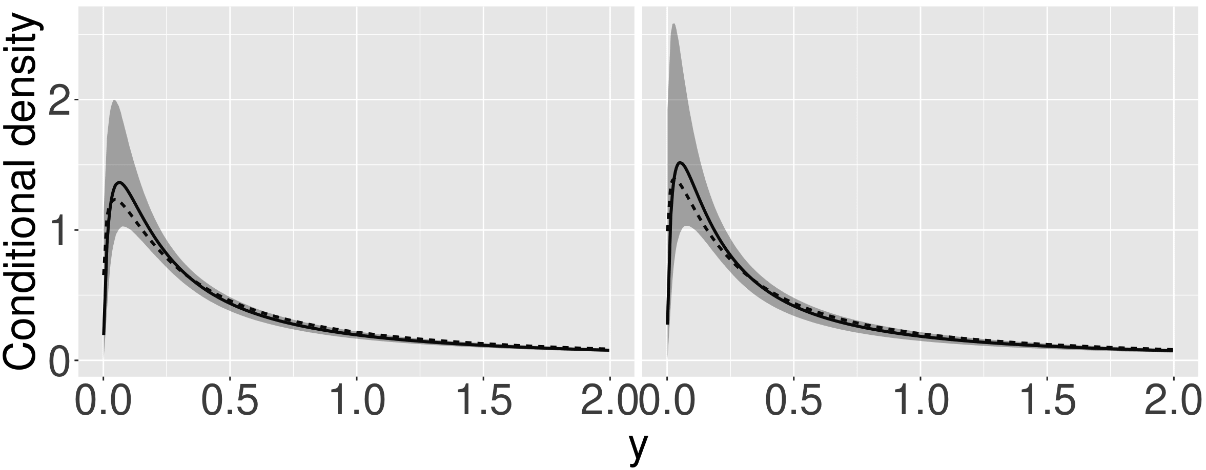
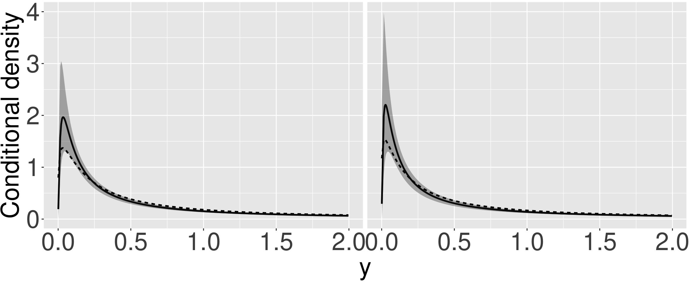
Scenario 3                                                           Scenario 4                 
(large effects for lower values, light effects for tail)        (large effects for lower values, large effects for tail)

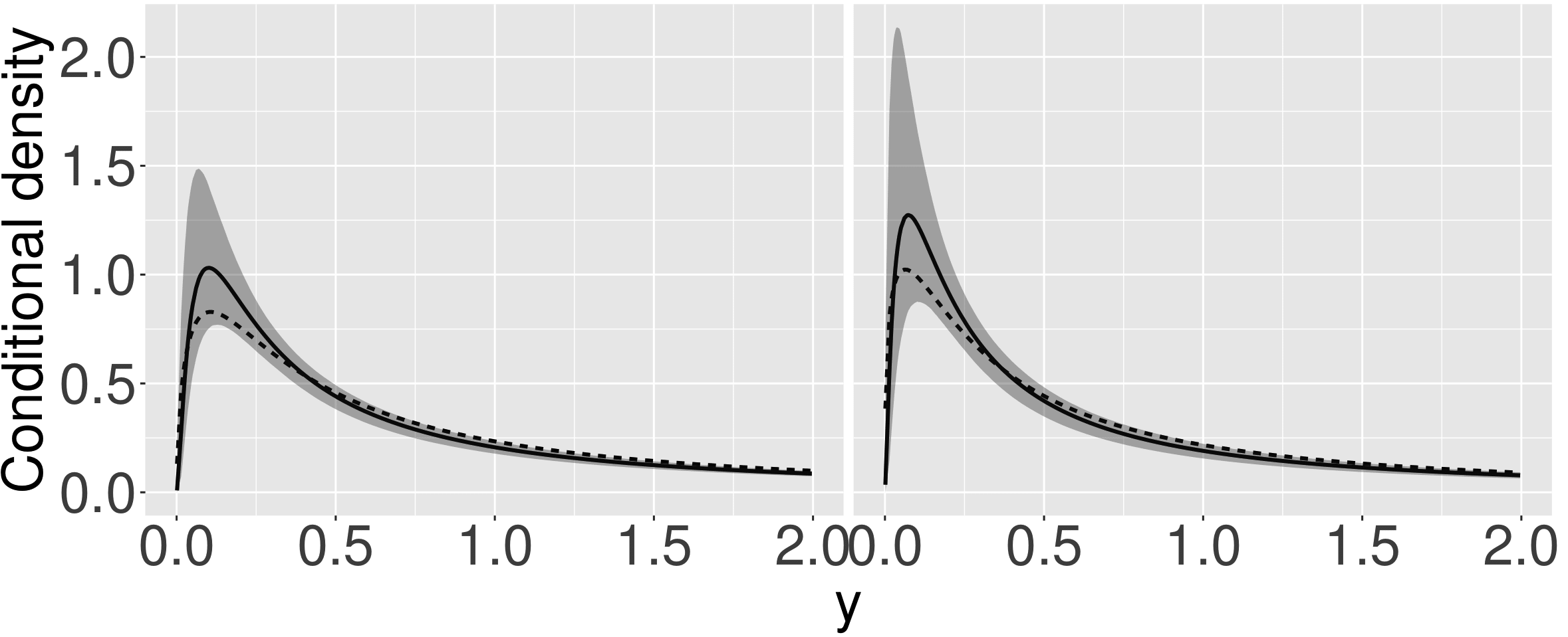
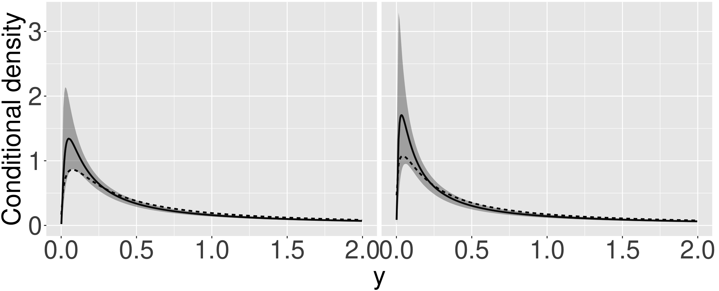
Figure 1: Cross sections of posterior mean conditional density (solid) along with pointwise credible bands against true (dashed) for a one-shot experiment with $n=500$; the cross sections result from conditioning on $\mathbf{x}=(0.25,\dots,0.25)$ (left) and $\mathbf{x}=(0.50,\dots,0.50)$ (right).

We consider four scenarios, described below, based on the following vectors for the regression coefficients:

• Scenario 1—Light effects for lower values, light effects for tail: $\bm{\beta}=\mathbf{a};\bm{\alpha}=\mathbf{b};\bm{\gamma}=\mathbf{c}$.

• Scenario 2—Light effects for lower values, large effects for tail: $\bm{\beta}=\mathbf{a};\alpha=2\mathbf{b};\gamma=2\mathbf{c}$

• Scenario 3—Large effects for lower values, light effects for tail: $\bm{\beta}=2\mathbf{a};\bm{\alpha}=b;\bm{\gamma}=\mathbf{c}$

• Scenario 4—Large effects for lower values, large effects for tail: $\bm{\beta}=2\mathbf{a};\alpha=2\mathbf{b};\gamma=2\mathbf{c}$

where $\mathbf{a}$, $\mathbf{b}$, $\mathbf{c}\in\mathbb{R}^{10}$ have components

$$a_{1}=a_{3}=0.3;a_{6}=a_{10}=-0.3;\quad b_{2}=-0.3;b_{5}=b_{8}=0.3;\quad c_{1}=c_{4}=c_{9}=0.3;c_{10}=-0.3;$$

and zero otherwise.

For each of the scenarios above, we simulated $n=500$ observations, $\{(\mathbf{x}_{i},y_{i})\}_{i=1}^{n}$, from a conditional EGPD with a canonical carrier function; this is about the same number of observations available in the data application of Section 4. The covariates are simulated from independent standard uniform distributions. Figure 1 shows cross sections of the true and conditional densities for Scenarios 1–4 estimated using our methods.

As can be seen from these figures, the method recovers satisfactorily well the true conditional density—especially keeping in mind the sample size.

Scenario 1
(light effects for lower values, light effects for tail)

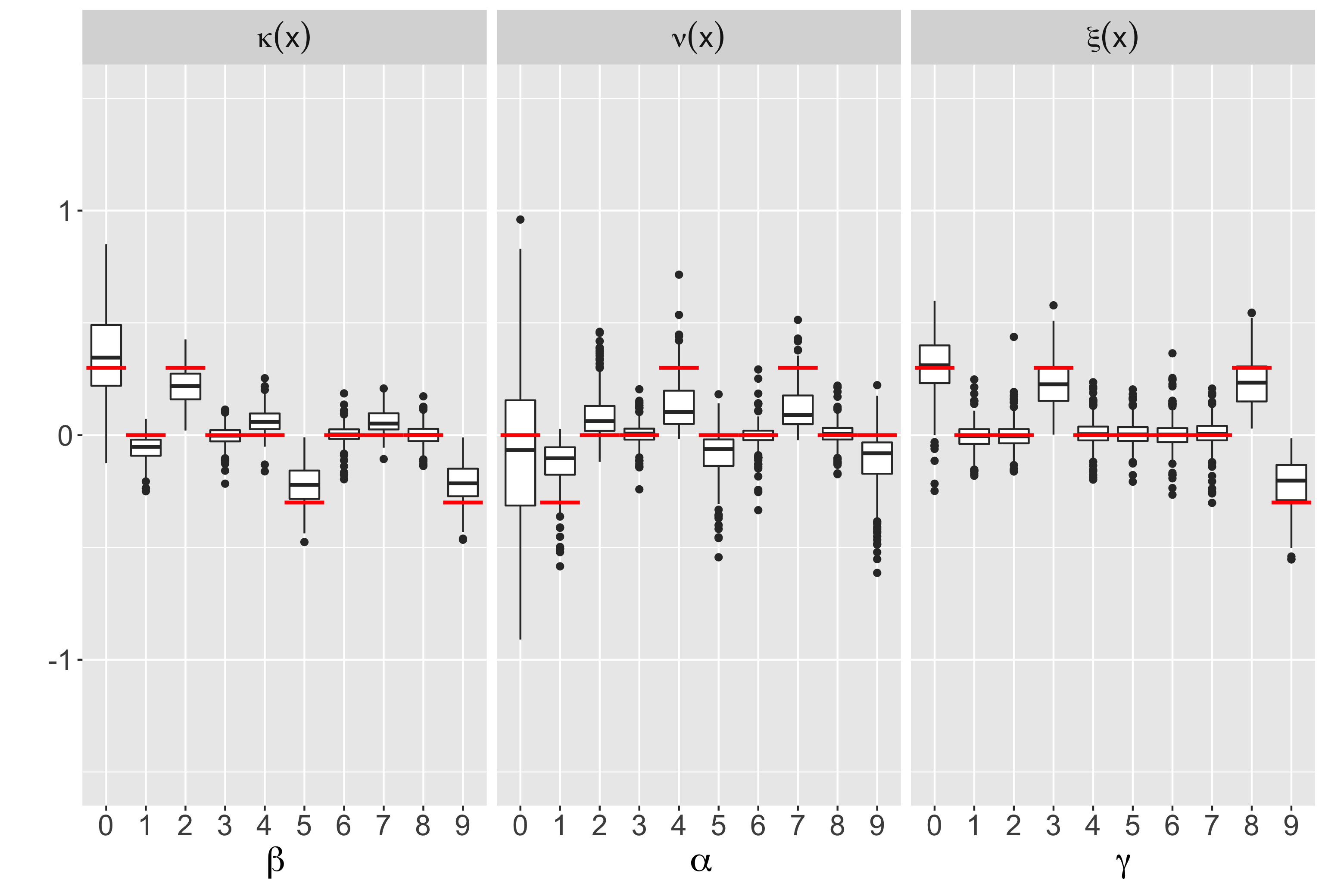
Scenario 2
(light effects for lower values, large effects for tail)

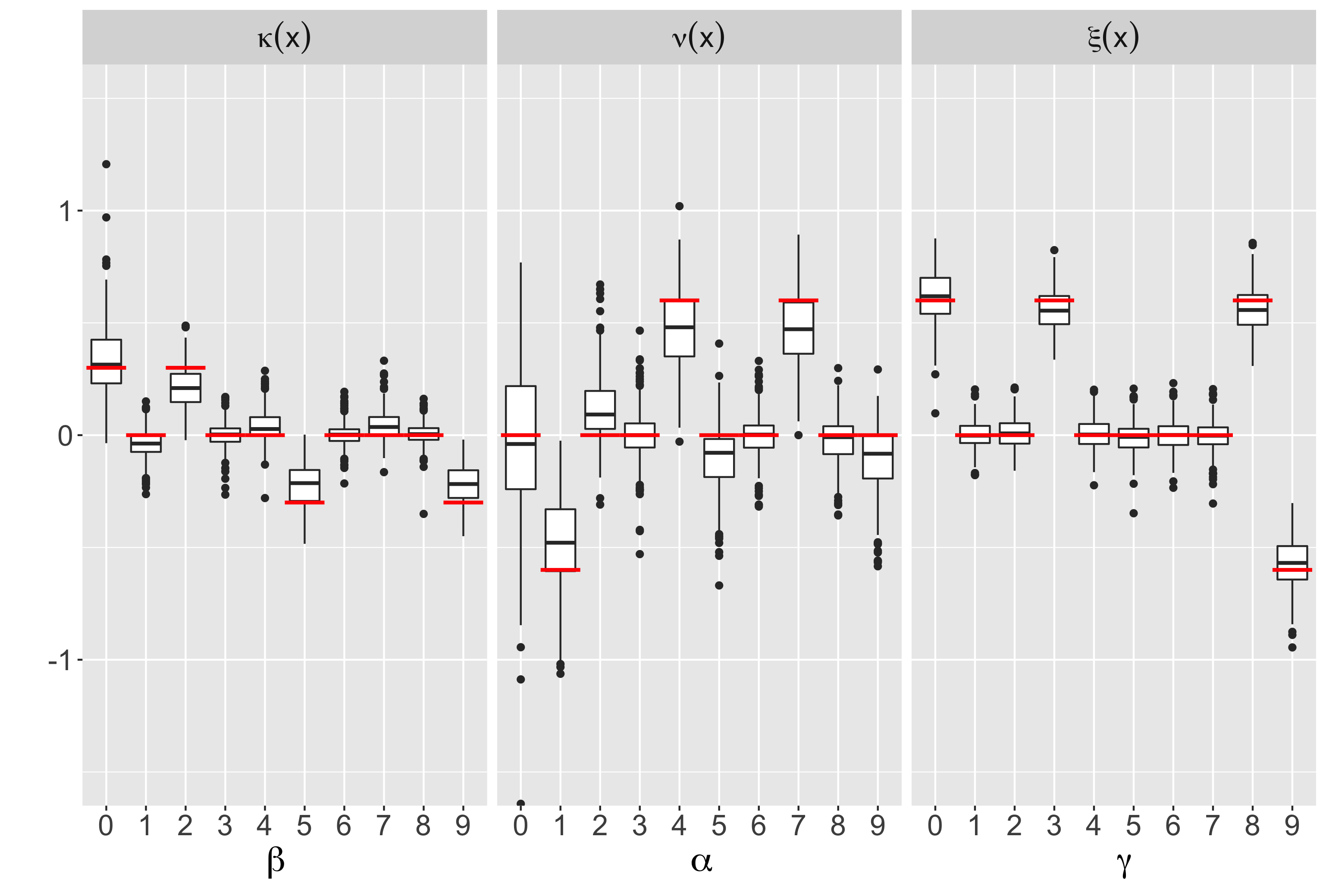
Scenario 3
(large effects for lower values, light effects for tail)

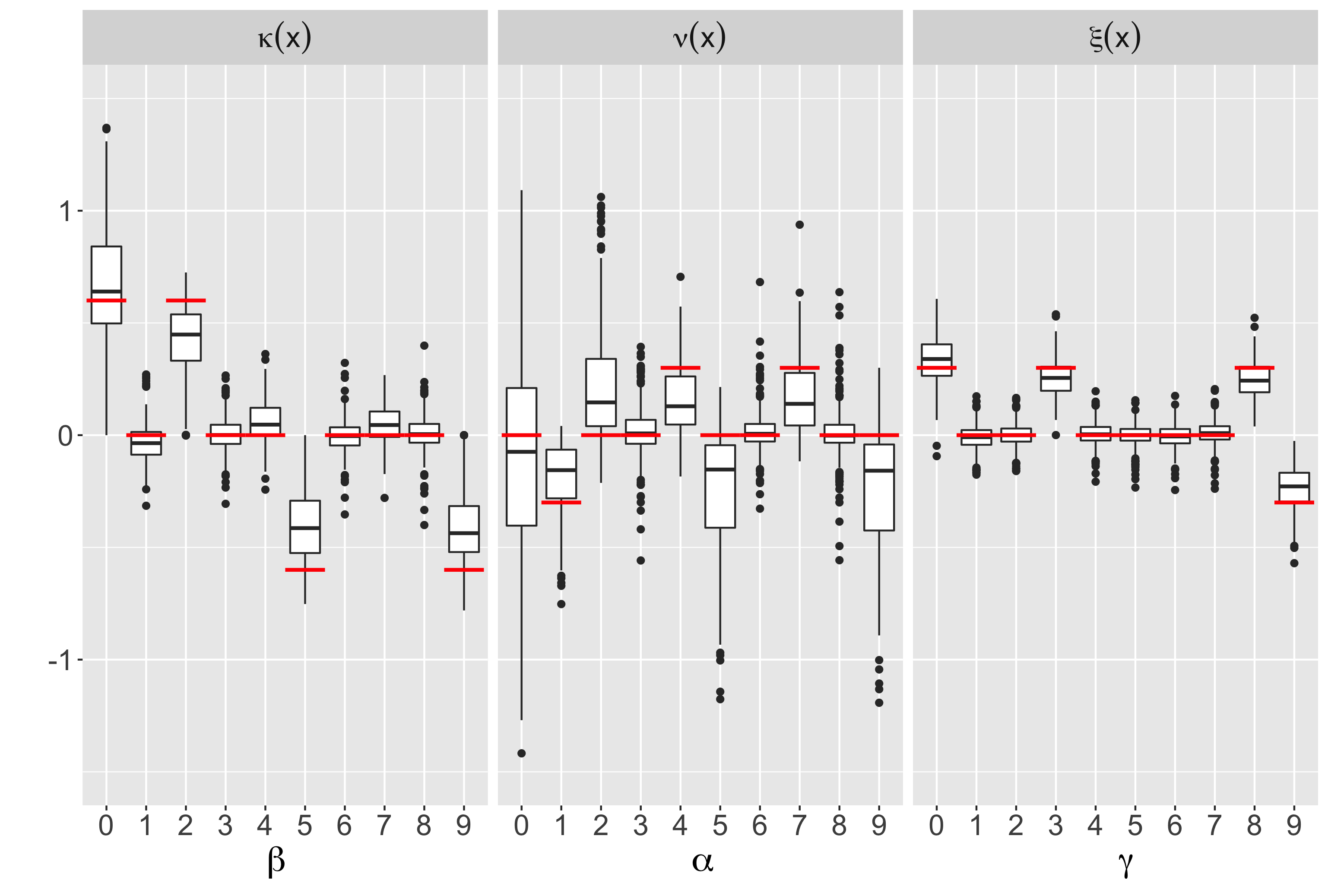
Scenario 4
(large effects for lower values, large effects for tail)

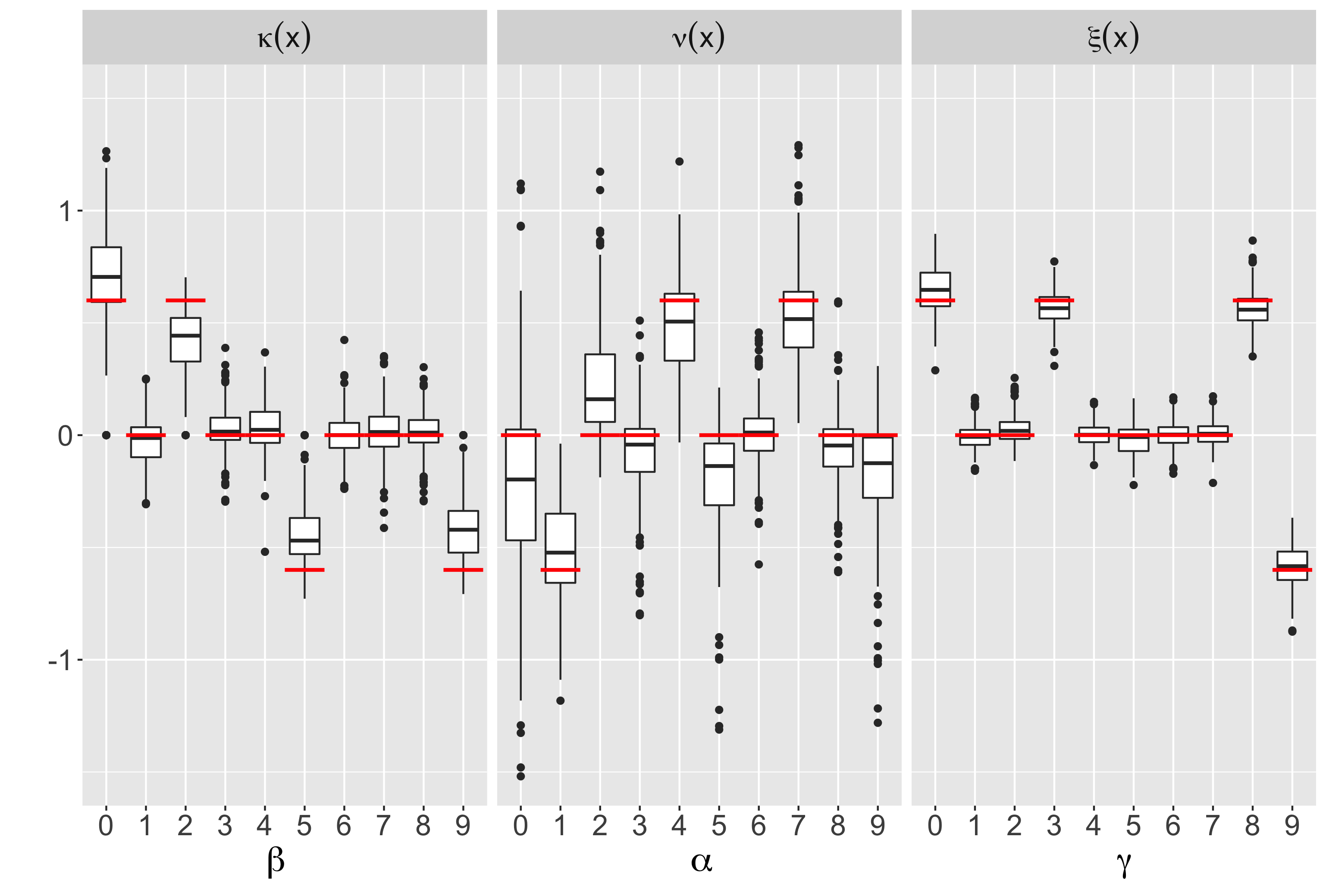
Figure 2: Side-by-side boxplots with regression coefficient estimates for Monte Carlo simulation study ($n=250$) plotted against the true values ( —). The values 1–9 represent the coefficient indices.

3.2 MONTE CARLO SIMULATION STUDY

To assess the finite-sample performance of the proposed methods, we now present the results of a Monte Carlo simulation study, where we repeat 250 times the one-shot experiments from Section 3.1. We consider the different sample sizes of $n=100$, $n=250$, and $n=500$.

Figure 2 presents side-by-side boxplots of the coefficient estimates for each scenario for the case $n=250$, and we can see that the estimates tend to be close to the true values thus suggesting that the proposed methods are able to learn what covariates are significant for the lower values, but not for the tail (and vice-versa); further simulation experiments (results not shown) indicate that performance may deteriorate if the number of common effects between left and right tails is large. The coefficient estimates for the cases $n=100$ and $n=500$ are reported in the Supplementary Material; as expected, the larger the sample size, the more accurate the estimates. The frequency of variable selection table presented in the Supplementary Material suggests a satisfactory performance of the method in terms of variable selection.

We now move to the conditional density. To compare the fitted conditional density against the true as the sample size increases, we resort to the mean integrated squared error (MISE):

$$\text{MISE}=\operatorname{E}\bigg{[}\int\int\{\widehat{f}(y\mid\mathbf{x})-f(y\mid\mathbf{x})\}^{2}\,\mathrm{d}\mathbf{x}\,\mathrm{d}y\bigg{]},$$

where the expectation is taken so to summarize the average behavior of the randomness on the double integral that stems from the posterior mean estimate $\widehat{f}$ (Wand and Jones, 1995, Section 2.3). Figure 4 shows a boxplot of the MISE of each run of the simulation experiment for Scenario 1. As can be seen from Figure 4, MISE tends to decrease as the sample size increases, thus indicating that a better performance of the proposed methods is to be expected on larger samples; the same holds for the remainder scenarios as can be seen from the boxplots of MISE available in the Supplementary Material. To examine the quality of each fit corresponding to a simulated dataset, $\{(\textbf{x}_{i},y_{i})\}_{i=1}^{n}$, we use randomized quantile residuals (Dunn and Smyth, 1996) adapted to our model, that is, $\{\varepsilon_{i}\}_{i=1}^{n}=[\Phi^{-1}\{\widehat{F}(y_{i}|\mathbf{x}_{i})\}]_{i=1}^{n}$, where $\Phi^{-1}$ is the quantile function of the standard Normal distribution and $\widehat{F}$ is the posterior mean estimate of the conditional distribution function. Figure 6 depicts the corresponding posterior mean QQ-plot of randomized quantile residuals against the theoretical standard normal quantiles, and it evidences an acceptably good fit of the model for Scenarios 1–4. Finally, to supplement the analysis, we also report in the Supplementary Material numerical experiments that tend to support the claim that the performance of the proposed methods is relatively satisfactory at separating covariate effects for the lower values and tail (Section 2.1 of Supplementary Material), and that this also holds in a misspecified setting. Despite the overall good performance, in all fairness not everything is perfect; specifically, our supporting numerical experiments reveal that: i) the correspondence between “non-constant” effects on lower quantiles and coefficients of $\kappa(\mathbf{x})$ is weaker for Scenario 3; ii) bias appears on the lower conditional quantile function estimates, under misspecification.

Scenario 1
(light effects for lower values, light effects for tail)

Scenario 2
(light effects for lower values, large effects for tail)

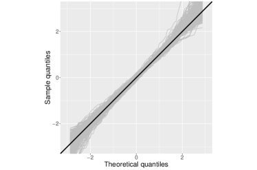
Scenario 3
(large effects for lower values, light effects for tail)

Scenario 4
(large effects for lower values, large effects for tail)

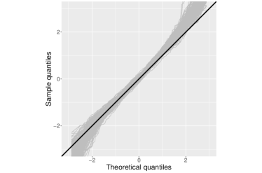
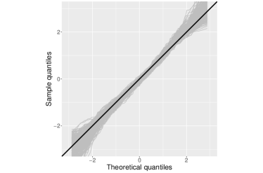
Figure 3: QQ-plots of randomized quantile residuals for Monte Carlo simulation study; each trajectory corresponds to a posterior mean QQ-plot from each simulated dataset.

Scenario 1
(light effects for lower values, light effects for tail)

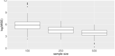
Figure 4: Side-by-side boxplots of MISE on the log scale for Monte Carlo simulation study for Scenario 1.

4 DRIVERS OF MODERATE AND EXTREME RAINFALL IN MADEIRA

4.1 MOTIVATION, APPLIED CONTEXT, AND DATA DESCRIPTION

We now showcase the proposed methodology with a climatological illustration with data from Funchal, Madeira (Portugal); the island of Madeira is an archipelago of volcanic origin located in the Atlantic Ocean about 900km southwest of mainland Portugal. Prior to fitting the proposed model, we start by providing some background on the scientific problem of interest and by describing the data. Madeira has suffered a variety of extreme rainfall events over the last two centuries, including the flash floods of October 1803 (800–1000 casualties) and those of February 2010—the latter with a death toll of 45 people (Fragoso et al., 2012; Santos et al., 2017) and with an estimated damage of 1.4 billion Euros (Baioni et al., 2011). Such violent rainfall events are often followed by damaging landslides events, including debris, earth, and mud flows.

To analyze such rainfall events in Funchal, Madeira, we have gathered data from the National Oceanic and Atmospheric Administration (www.noaa.gov). Specifically, we have gathered total monthly precipitation (.01 inches), as well as the following potential drivers for extreme rainfall: Atlantic multi-decadal Oscillation (AMO), El Niño-Southern Oscillation (expressed by NINO34 index) (ENSO), North Pacific Index (NP), Pacific Decadal Oscillation (PDO), Southern Oscillation Index (SOI), and North Atlantic Oscillation (NAO). The sample period covers January 1973 to June 2018, thus including episodes such as the violent flash floods of 1979, 1993, 2001, and 2010 (Baioni et al., 2011). After eliminating the dry events (i.e., zero precipitation) and the missing precipitation data (two observations), we are left with a total of 532 observations.

The potential drivers for extreme rainfall above have been widely examined in the climatological literature, mainly on large landmasses. In particular, it has been suggested that in North America ENSO, PDO, and NAO play a key role governing the occurrence of extreme rainfall events (Kenyon and Hegerl, 2010; Zhang et al., 2010; Whan and Zwiers, 2017); yet for the UK, while NAO is believed to impact the occurrence of extreme rainfall events, no influence of PDO nor AMO has been detected (Brown, 2018). The many peculiarities surrounding Madeira climate (e.g., Azores Anticyclone, Canary Current, Gulf Stream, etc.), along with the negative impact that flash floods and landslide events produce on the island, motivate us to ask: i) whether such drivers are relevant for explaining extreme rainfall episodes in Madeira; ii) whether such drivers are also relevant for moderate rainfall events.

4.2 TRACKING DRIVERS OF MODERATE AND EXTREME RAINFALL

One of the goals of the analysis is to use the lenses of our model so to learn what are the drivers of moderate and extreme rainfall in Funchal. To conduct such inquiry, we use the full model from Section 2.4 (see Eq. (9)), with power carrier $G_{\kappa(\mathbf{x})}(v)=v^{\kappa(\mathbf{x})}$ and with link functions

$$\kappa(\mathbf{x})=\exp(\mathbf{x}^{\mathrm{\scriptscriptstyle T}}\bm{\beta}),\quad\nu(\mathbf{x})=\exp(\mathbf{x}^{\mathrm{\scriptscriptstyle T}}\bm{\alpha}),\quad\xi(\mathbf{x})=\mathbf{x}^{\mathrm{\scriptscriptstyle T}}\bm{\gamma}.$$

Covariates have been standardized and we used a flat Normal prior, $\text{N}(0,100^{2})$, for the intercepts, and uninformative Gamma priors, $\operatorname{Gamma}(0.1,0.1)$, for the hyperparameters $\lambda_{k}$, $\lambda_{\nu}$, $\lambda_{\xi}$; here an identity link was used for $\xi(\mathbf{x})$ as fitting a GPD to the response via likelihood methods suggested no compelling evidence in favor of an heavy-tailed response. After a burn-in period of 10 000 iterations, we collected a total of 20 000 posterior samples. The results of MCMC convergence diagnostics were satisfactory; in particular, the effective sample sizes were acceptably high, ranging from about 1000 to 5 000, and all values of Geweke’s diagnostic were satisfactory, ranging from about $-3.2$ to $3.0$. Figure 5 depicts the credible intervals for each regression coefficient. To assess the fit of the proposed model we resort once more to randomized quantile residuals (Dunn and Smyth, 1996). Figure 6 evidences an acceptably good fit of the model; while the pointwise bands in Figure 6 are narrow, they result from acceptably high effective sample sizes as mentioned above.

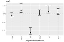
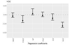
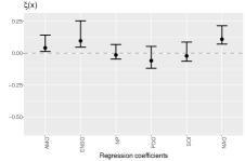
Figure 5: Credible intervals for regression coefficients for inverse-link functions; the dots ($\bullet$) represent the posterior means and the dashed line represents the reference line $\beta=0$.

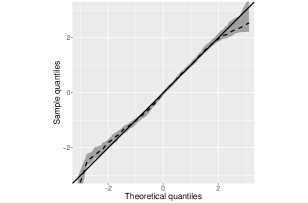
Figure 6: QQ-plot of randomized quantile residuals; the dashed line represents the posterior mean plotted along with pointwise credible bands.

Figure 5 (middle and right panels) suggests that the key drivers for extreme rainfall in Funchal are NAO and ENSO, along with a possible modest influence of AMO on the magnitude of extreme rainfall events. To put it differently, such results hint that a higher NAO, ENSO, and AMO tend to be associated with extreme rainfall episodes in Funchal. Such findings are thus reasonably in line with those of Kenyon and Hegerl (2010) Zhang et al. (2010), and Whan and Zwiers (2017) for North America. Yet, similarly to Brown (2018), we find no relevant impact of PDO, given the rest, on extreme rainfall spells. Interestingly, of all these potencial drivers for extreme rainfall, only ENSO seems to be statistically associated with moderate rainfall; see Figure 5 (left). Also, NP is the most relevant driver of moderate rainfall, and yet the analysis suggests it plays no role on extreme rainfall. Additionally, Figure 5 (left) suggests that an increase in NP leads to a heavier left tail (i.e., dryer months), whereas an increase in ENSO leads to less mass close to zero (i.e., rainy months). Finally, to supplement the analysis, we also present conditional quantiles in the Supplementary Material so to directly assess how rainfall itself is impacted by all these potential drivers.

5 CLOSING REMARKS

In this paper we have introduced a Lasso-type model for the lower values and tail of a possibly heavy-tailed response. The proposed model: i) bypasses the need for threshold selection ($u_{\mathbf{x}}$); ii) models both the conditional lower values and conditional tails; iii) it is naturally tailored for variable selection. In addition, contrarily to GPD-based approach of Davison and Smith (1990) the proposed model does not suffer from lack of threshold stability, as indeed our model does not depend on a threshold; the fact that the Davison–Smith approach does not retain the threshold stability property is known since (Eastoe and Tawn, 2009, Section 2.2), and it implies that selection of covariates in the parameters of the GPD is not invariant to threshold choice. Yet, other approaches that circumvent the threshold stability issue are available beyond our model, including an inhomogeneous point process formulation for extremes (Coles, 2001, Chapter 7). Interestingly, the proposed model can be regarded as a Lasso-type model for quantile regression that is tailored for both the lower values and for extrapolating into the tails. As a byproduct, our paper has links with the Bayesian literature on Bayesian distributional regression (Umlauf and Kneib, 2018), and with the recent paper of Groll et al. (2019).

Despite the considerations above on threshold selection there is no ‘free lunch’; indeed, here the parameters of the model and the choice of the carrier dictate the behavior of the quantiles in the whole range of the distribution, while the impact of some parameters is smaller in the lower or upper tail. Yet, competing EGPD models that stem from different choices for the carrier function can be formally compared and ranked via standard model selection criteria, such as Log Pseudo Marginal Likelihood (e.g. Geisser and Eddy, 1979; Gelfand and Dey, 1994).

Some final comments on future research are in order. A version of our model that includes additionally a regression model for point masses at zero would be natural for a variety of contexts, such as for modeling long periods without rain or droughts. Semicontinuous responses that consist of a mixture of zeros and a continuous positive distribution are indeed common in practice (e.g., Olsen and Schafer, 2001). Another natural avenue for future research would endow the model with further flexibility by resorting to a generalized additive model, where the smooth function of each covariate is modeled using B-spline basis functions. The latter extension would however require a group lasso (Yuan and Lin, 2006), shrinking groups of regression coefficients (per smooth function) towards zero. While we focus here on modeling positive random variables, another interesting extension of the proposed model would consider the left endpoint itself as a parameter rather than fixing it at zero. Finally, from an inference perspective it would also seem natural defining a semiparametric Bayesian version of our model that would set a prior directly on the covariate-specific carrier function $G_{\mathbf{x}}$ rather than specifying a power carrier function in advance, and to model the conditional density as $F(y\mid\mathbf{x})=G_{\mathbf{x}}{\{H(y\mid\mathbf{x})\}}$. This approach would however require setting a prior on the space $\mathscr{G}$ of all carrier functions so as to ensure that $G_{\mathbf{x}}$ obeys Assumptions A–C, for all $\mathbf{x}$. While priors on spaces of functions are an active field of research (Ghosal and Van der Vaart, 2015), definition of priors over $\mathscr{G}$ is to our knowledge an open problem; a natural line of attack to construct such a prior would be via random Bernstein polynomials (Petrone and Wasserman, 2002), with weight constraints derived from Lemma 1 of Tencaliec et al. (2019); indeed, by modeling the carrier function with a Bernstein polynomial basis a higher level of flexibility could be achieved in comparison to that offered by Examples 1–3.

REFERENCES

- Arnold and Press (1989) Arnold, B. C. and Press, S. J. (1989), Bayesian estimation and prediction for Pareto data, Journal of the American Statistical Association, 84, 1079–1084.
- Baioni et al. (2011) Baioni, D., Castaldini, D., and Cencetti, C. (2011), Human activity and damaging landslides and floods on Madeira Island. Natural Hazards & Earth System Sciences, 11, 3035–3046.
- Behrens et al. (2004) Behrens, C. N., Lopes, H. F., and Gamerman, D. (2004), Bayesian analysis of extreme events with threshold estimation, Statistical Modelling, 4, 227–244.
- Beirlant et al. (2004) Beirlant, J., Goegebeur, Y., Segers, J., and Teugels, J. (2004), Statistics of Extremes: Theory and Applications, Wiley, Hoboken, NJ: Wiley.
- Bhattacharya et al. (2015) Bhattacharya, A., Pati, D., Pillai, N. S., and Dunson, D. B. (2015), Dirichlet–Laplace priors for optimal shrinkage, Journal of the American Statistical Association, 110, 1479–1490.
- Brown (2018) Brown, S. J. (2018), The drivers of variability in UK extreme rainfall, International Journal of Climatology, 38, e119–e130.
- Cabras and Castellanos (2011) Cabras, S. and Castellanos, M. E. (2011), A Bayesian approach for estimating extreme quantiles under a semiparametric mixture model, ASTIN Bulletin, 41, 87–106.
- Carreau and Bengio (2009) Carreau, J. and Bengio, Y. (2009), A hybrid Pareto model for asymmetric fat-tailed data: The univariate case, Extremes, 12, 53–76.
- Carvalho et al. (2010) Carvalho, C. M., Polson, N. G., and Scott, J. G. (2010), The horseshoe estimator for sparse signals, Biometrika, 97, 465–480.
- Castellanos and Cabras (2007) Castellanos, M. E. and Cabras, S. (2007), A default Bayesian procedure for the generalized Pareto distribution, Journal of Statistical Planning and Inference, 137, 473–483.
- Chavez-Demoulin and Davison (2005) Chavez-Demoulin, V. and Davison, A. C. (2005), Generalized additive modelling of sample extremes, Journal of the Royal Statistical Society: Series C (Applied Statistics), 54, 207–222.
- Chavez-Demoulin et al. (2016) Chavez-Demoulin, V., Embrechts, P., and Hofert, M. (2016), An extreme value approach for modeling operational risk losses depending on covariates, Journal of Risk and Insurance, 83, 735–776.
- Chernozhukov (2005) Chernozhukov, V. (2005), Extremal quantile regression, Annals of Statistics, 33, 806–839.
- Coles (2001) Coles, S. (2001), An Introduction to Statistical Modeling of Extreme Values, London: Springer.
- Davison and Smith (1990) Davison, A. C. and Smith, R. L. (1990), Models for exceedances over high thresholds (with Discussion), Journal of the Royal Statistical Society: Series B (Statistical Methodology), 393–442.
- de Zea Bermudez and Kotz (2010) de Zea Bermudez, P. and Kotz, S. (2010), Parameter estimation of the generalized Pareto distribution—Part II, Journal of Statistical Planning and Inference, 140, 1374–1388.
- de Zea Bermudez and Turkman (2003) de Zea Bermudez, P. and Turkman, M. A. (2003), Bayesian approach to parameter estimation of the generalized Pareto distribution, Test, 12, 259–277.
- do Nascimento et al. (2012) do Nascimento, F. F., Gamerman, D., and Lopes, H. F. (2012), A semiparametric Bayesian approach to extreme value estimation, Statistics and Computing, 22, 661–675.
- Dunn and Smyth (1996) Dunn, P. K. and Smyth, G. K. (1996), Randomized quantile residuals, Journal of Computational and Graphical Statistics, 5, 236–244.
- Eastoe and Tawn (2009) Eastoe, E. F. and Tawn, J. A. (2009), Modelling non-stationary extremes with application to surface level ozone, Journal of the Royal Statistical Society: Series C (Applied Statistics), 58, 25–45.
- Embrechts et al. (1997) Embrechts, P., Klüppelberg, C., and Mikosch, T. (1997), Modelling Extremal Events for Insurance and Finance, New York: Springer.
- Fragoso et al. (2012) Fragoso, M., Trigo, R., Pinto, J., Lopes, S., Lopes, A., Ulbrich, S., and Magro, C. (2012), The 20 February 2010 Madeira flash-floods: synoptic analysis and extreme rainfall assessment, Natural Hazards and Earth System Sciences, 12, 715–730.
- Frigessi et al. (2002) Frigessi, A., Haug, O., and Rue, H. (2002), A dynamic mixture model for unsupervised tail estimation without threshold selection, Extremes, 5, 219–235.
- Geisser and Eddy (1979) Geisser, S. and Eddy, W. F. (1979), A predictive approach to model selection, Journal of the American Statistical Association, 74, 153–160.
- Gelfand and Dey (1994) Gelfand, A. E. and Dey, D. K. (1994), Bayesian model choice: asymptotics and exact calculations, Journal of the Royal Statistical Society: Series B (Statistical Methodology), 56, 501–514.
- Gelman et al. (2015) Gelman, A., Lee, D., and Guo, J. (2015), Stan: A probabilistic programming language for Bayesian inference and optimization, Journal of Educational and Behavioral Statistics, 40, 530–543.
- George and McCulloch (1993) George, E. I. and McCulloch, R. E. (1993), Variable selection via Gibbs sampling, Journal of the American Statistical Association, 88, 881–889.
- Ghosal and Van der Vaart (2015) Ghosal, S. and Van der Vaart, A. W. (2015), Fundamentals of Nonparametric Bayesian Inference, Cambridge University Press, Cambridge.
- Groll et al. (2019) Groll, A., Hambuckers, J., Kneib, T., and Umlauf, N. (2019), LASSO-type penalization in the framework of generalized additive models for location, scale and shape, Computational Statistics & Data Analysis, 140, 59–73.
- Huser and Genton (2016) Huser, R. and Genton, M. G. (2016), Non-stationary dependence structures for spatial extremes, Journal of Agricultural, Biological, and Environmental Statistics, 21, 470–491.
- Kenyon and Hegerl (2010) Kenyon, J. and Hegerl, G. C. (2010), Influence of modes of climate variability on global precipitation extremes, Journal of Climate, 23, 6248–6262.
- Kleiber and Kotz (2003) Kleiber, C. and Kotz, S. (2003), Statistical Size Distributions in Economics and Actuarial Sciences, New York: Wiley.
- Koenker (2005) Koenker, R. (2005), Quantile Regression, Cambridge, MA: Cambridge University Press.
- Koenker and Bassett (1978) Koenker, R. and Bassett, G. (1978), Regression quantiles, Econometrica, 33–50.
- MacDonald et al. (2011) MacDonald, A., Scarrott, C., Lee, D., Darlow, B., Reale, M., and Russell, G. (2011), A flexible extreme value mixture model, Computational Statistics & Data Analysis, 55, 2137–2157.
- Mahmoud and Abd El-Ghafour (2015) Mahmoud, M. R. and Abd El-Ghafour, A. S. (2015), Fisher information matrix for the generalized Feller–Pareto distribution, Communications in Statistics—Theory and Methods, 44, 4396–4407.
- Naveau et al. (2016) Naveau, P., Huser, R., Ribereau, P., and Hannart, A. (2016), Modeling jointly low, moderate, and heavy rainfall intensities without a threshold selection, Water Resources Research, 52, 2753–2769.
- Olsen and Schafer (2001) Olsen, M. K. and Schafer, J. L. (2001), A two-part random-effects model for semicontinuous longitudinal data, Journal of the American Statistical Association, 96, 730–745.
- Papastathopoulos and Tawn (2013) Papastathopoulos, I. and Tawn, J. A. (2013), Extended generalised Pareto models for tail estimation, Journal of Statistical Planning and Inference, 143, 131–143.
- Park and Casella (2008) Park, T. and Casella, G. (2008), The Bayesian Lasso, Journal of the American Statistical Association, 103, 681–686.
- Petrone and Wasserman (2002) Petrone, S. and Wasserman, L. (2002), Consistency of Bernstein polynomial posteriors, Journal of the Royal Statistical Society: Series B (Statistical Methodology), 64, 79–100.
- Plummer (2019) Plummer, M. (2019), rjags: Bayesian graphical models using MCMC. R package version 4-10, http://CRAN.R-project.org/package=rjags, .
- Polson and Sokolov (2019) Polson, N. G. and Sokolov, V. (2019), Bayesian regularization: From Tikhonov to horseshoe, Wiley Interdisciplinary Reviews: Computational Statistics, e1463.
- Reich and Ghosh (2019) Reich, B. J. and Ghosh, S. K. (2019), Bayesian Statistical Methods, Boca Raton, FL: Chapman & Hall/CRC.
- Resnick (1971) Resnick, S. I. (1971), Tail equivalence and its applications, Journal of Applied Probability, 8, 136–156.
- Santos et al. (2017) Santos, M., Santos, J. A., and Fragoso, M. (2017), Atmospheric driving mechanisms of flash floods in Portugal, International Journal of Climatology, 37, 671–680.
- Schott (2016) Schott, J. R. (2016), Matrix Analysis for Statistics, New York: Wiley.
- Stein (2020) Stein, M. L. (2020), Parametric models for distributions when interest is in extremes with an application to daily temperature, Extremes, 1–31.
- Stein (2021) — (2021), A parametric model for distributions with flexible behavior in both tails, Environmetrics, 32, e2658.
- Tencaliec et al. (2019) Tencaliec, P., Favre, A.-C., Naveau, P., Prieur, C., and Nicolet, G. (2019), Flexible semiparametric Generalized Pareto modeling of the entire range of rainfall amount, Environmetrics, e2582.
- Tibshirani (1996) Tibshirani, R. (1996), Regression shrinkage and selection via the Lasso, Journal of the Royal Statistical Society: Series B (Statistical Methodology), 58, 267–288.
- Umlauf and Kneib (2018) Umlauf, N. and Kneib, T. (2018), A primer on Bayesian distributional regression, Statistical Modelling, 18, 219–247.
- Villa (2017) Villa, C. (2017), Bayesian estimation of the threshold of a generalised Pareto distribution for heavy-tailed observations, Test, 26, 95–118.
- Wand and Jones (1995) Wand, M. P. and Jones, M. C. (1995), Kernel Smoothing, London: Chapman & Hall, 1st ed.
- Wang and Tsai (2009) Wang, H. and Tsai, C.-L. (2009), Tail index regression, Journal of the American Statistical Association, 104, 1233–1240.
- Whan and Zwiers (2017) Whan, K. and Zwiers, F. (2017), The impact of ENSO and the NAO on extreme winter precipitation in North America in observations and regional climate models, Climate Dynamics, 48, 1401–1411.
- Young and Smith (2005) Young, G. A. and Smith, R. L. (2005), Essentials of Statistical Inference, Cambridge, UK: Cambridge University Press.
- Yuan and Lin (2006) Yuan, M. and Lin, Y. (2006), Model selection and estimation in regression with grouped variables, Journal of the Royal Statistical Society: Series B (Statistical Methodology), 68, 49–67.
- Zhang et al. (2010) Zhang, X., Wang, J., Zwiers, F. W., and Groisman, P. Y. (2010), The influence of large-scale climate variability on winter maximum daily precipitation over North America, Journal of Climate, 23, 2902–2915.
- Zhang et al. (2020) Zhang, Y. D., Naughton, B. P., Bondell, H. D., and Reich, B. J. (2020), Bayesian regression using a prior on the model fit: The R2-D2 shrinkage prior, Journal of the American Statistical Association, 1–13.