A Data Driven End-to-end Approach for In-the-wild Monitoring of Eating Behavior Using Smartwatches

Abstract

The increased worldwide prevalence of obesity has sparked the interest of the scientific community towards tools that objectively and automatically monitor eating behavior. Despite the study of obesity being in the spotlight, such tools can also be used to study eating disorders (e.g. anorexia nervosa) or provide a personalized monitoring platform for patients or athletes. This paper presents a complete framework towards the automated i) modeling of in-meal eating behavior and ii) temporal localization of meals, from raw inertial data collected in-the-wild using commercially available smartwatches. Initially, we present an end-to-end Neural Network which detects food intake events (i.e. bites). The proposed network uses both convolutional and recurrent layers that are trained simultaneously. Subsequently, we show how the distribution of the detected bites throughout the day can be used to estimate the start and end points of meals, using signal processing algorithms. We perform extensive evaluation on each framework part individually. Leave-one-subject-out (LOSO) evaluation shows that our bite detection approach outperforms four state-of-the-art algorithms towards the detection of bites during the course of a meal (0.923 F1 score). Furthermore, LOSO and held-out set experiments regarding the estimation of meal start/end points reveal that the proposed approach outperforms a relevant approach found in the literature (Jaccard Index of 0.820 and 0.821 for the LOSO and held-out experiments, respectively). Experiments are performed using our publicly available FIC and the newly introduced FreeFIC datasets.

I Introduction

Reports published by the World Health Organization (WHO) formally recognized the global epidemic status of obesity [1]. Regardless of the extensive research that has been conducted over the years towards understanding obesity, the reasons behind why people gain excessive weight are still not completely understood [2]. Yet, the positive energy balance, or in other words when the input energy to one’s body exceeds the output, explains many of the metabolic, endocrine and behavioral aspects of weight gain [2, 1].

Currently, the most common way of objectively and automatically measuring one’s energy expenditure in free-living conditions is done via physical activity monitoring with the use of accelerometers [3, 4]. Even though the field is still under active research, many solutions have reached product-level quality, such as Fitbit, Google Fit, Samsung’s S Health and Apple’s Health.

At the same time, the food diary is still the most common way of monitoring one’s eating habits. Despite being easy to use, the food diary can suffer in terms of accuracy [5], capacity to measure certain eating behavior parameters that are linked with obesity such as eating rate [6] and low compliance [7]. The lack of tools as well as the plethora of available sensing devices in the market motivated the research community to explore automated and objective monitoring solutions [8, 7] both for the in-meal and for the less constrained, in-the-wild measurement of eating behavior. Besides the study of obesity, there are multiple domains that can also benefit from the development of automatic and objective behavior monitoring tools including, but not limited to, the study of eating disorders (e.g. anorexia nervosa) and the personalized monitoring for patients or athletes.

Different solutions for measuring in-meal eating behavior have been proposed in the recent literature. For example, the works of [9, 10, 11] use the information from wrist-mounted inertial sensors to detect food intake moments. Plate-like weight sensors [12, 6] can estimate the weight of each individual bite taken throughout the meal. Audio sensors allow the detection of chewing events [13, 14] and the recognition of various food types [14]. More complex sensors like cameras can recognize food types [15, 16, 17] and estimate the caloric intake of a meal by taking pictures of the plate before and after eating [18].

A more challenging problem arises when dealing with in-the-wild recordings where meals are only a small part of the recorded data. In such occasions, special care must be taken in order to maintain high performance while at the same time keep false positives and false negatives, that can occur during free-living activities, as low as possible. For example, the works of [19, 20] use a in-ear microphone to detect chewing events under free-living conditions. Inertial information from wrist-mounted sensors can also be used in order to detect eating [21, 22] and liquid intake episodes [23]. The work presented in [24] uses a novel segmentation technique for the detection and recognition of eating and drinking gestures from continuous IMU data recorded in free-living conditions. Fusing inertial and audio information has also shown promising results in the works of [25, 26]. Additionally, the work presented in [27] showcases how the combination of free-living and laboratory data with information from both audio and inertial body-worn sensors can help recognize eating moments. Eating behavior modeling under free-living conditions can also be achieved using wearable cameras [28] and jaw motion sensors [29]. Finally, the authors of [30] combine the information from body-worn audio and inertial sensors and use a semi-supervised hierarchical classification scheme to identify the food type in unrestricted environments.

In this paper we propose a complete framework for automatically measuring eating behavior from in-the-wild collected inertial data (acceleration and orientation velocity) using a smartwatch. Initially, we show how a purely data-driven approach that uses an end-to-end Neural Network (NN) with both convolutional and recurrent layers can be used to detect food intake events (i.e. bites). Then we present how the distribution of detected bites throughout the day can be used to isolate meal events and detect their start and end time-points. In our experimental section we extensively evaluate each part of the framework individually, in terms of in-meal bite detection and in terms of detecting meal end-points under free-living conditions, and compare it with other state-of-the-art approaches found in the literature. In all experiments we use our Food Intake Cycle (FIC) and the newly introduced FreeFIC datasets. Both datasets are publicly available on the Multimedia Understanding Group webpage.

The rest of the paper is organized as follows. Section II provides a review of the relevant work regarding: i) the in-meal detection of eating moments and ii) the localization of eating events throughout the day using in-the-wild collected data. Sections III and IV describe the steps of the proposed data driven bite detection and meal localization approaches. Section V presents the datasets, the experiments and results. Section VI presents the limitations of the proposed approach. Finally, Section VII concludes the paper.

II Related work

A number of works have been proposed in the recent literature [31] for measuring in-meal eating behavior by detecting food intake events using inertial data from wrist mounted sensors. The common denominator between such works is that they aim at recognizing specific wrist movements (or series of wrist movements) that are part of the process of delivering food to the mouth.

The authors of [11] use a single gyroscope channel to detect a characteristic wrist-roll motion that happens during a bite event. The same algorithm was used to produce the results presented in [32]. Specifically, a bite is detected as a sequence of four different conditions. The first two conditions have to do with the velocity initially surpassing a positive and then a negative threshold. The final two conditions deal with the minimum amount of time that needs to pass between the two aforementioned roll motions and between two consecutive detected bites. The authors of [32] report a sensitivity/positive predictive value of $0.81$/$0.86$ using data collected in the lab and $0.81$/$0.83$ using more realistic data collected in the cafeteria.

The most recent work of our group [10], proposes an in-meal bite detection method that uses the inertial data ($3$D acceleration and orientation velocity) from off-the-shelf smartwatches. In more detail, we use five specific wrist micromovements (namely pick food, upwards, downwards, mouth and no movement) to model the series of actions leading to and following an intake event. The method operates in two steps. In the first step we process windows of raw sensor data to estimate the micromovement probability distribution using a Convolutional Neural Network (CNN). During the second step, we use a Long-short Term Memory (LSTM) network to capture the temporal evolution of micromovements and classify sequences as food intakes cycles. Leave-one-subject-out (LOSO) evaluation results on our public FIC dataset of $21$ meals from $12$ subjects yield a promising F$1$ score of $0.913$. Despite the satisfying performance, annotating micromovements in IMU sequences using visual information is an expensive and error-prone process.

An approach that revolves around a similar micromovement-based concept as [10] is presented by Zhang et al. in [9]. The authors propose the use of two wrist gestures in order to characterize a motion as a feeding gesture, namely: “food to mouth” and “back to rest”. Their processing pipeline starts by preprocessing the acceleration and orientation velocity streams, continues with the extraction of $66$ statistical features using a sliding window approach and a classification scheme to characterize windows as feeding or non-feeding gestures. Finally, bite detection is achieved by clustering the detected feeding gestures using Density-Based Spatial Clustering of Applications with Noise (DBSCAN). The authors evaluate their algorithm using a leave-one-subject-out cross validation scheme on their dataset of $15$ subjects. In their experimental section, the authors report an F$1$ score of $0.757$ using the AdaBoost classifier and the most descriptive feature subset.

In another work of our group [33] we present a data-driven approach towards the detection of bites during the course of a meal without using the additional knowledge of micromovements. The core of our approach is an Artificial Neural Network (ANN) with convolutional and recurrent layers. Experimental results with a smaller version of the FIC dataset ($10$ meals from $10$ subjects) showed that the data-driven method achieved similar performance as a micromovement-based approach [34], with F$1$ scores of $0.884$ and $0.892$ respectively. In the work presented in this paper we further expand the works of [34, 33] by increasing the knowledge base of the model and moving further way from a micromovement-based approach. This allows the convolutional part of the network to discover the optimal features representations before performing temporal modeling using an LSTM.

The approaches discussed so far focus on measuring and modeling in-meal eating behavior i.e., behavior during the course of a meal. On the other hand, a much smaller body of research aims at identifying and localizing eating episodes (such as meals or snacks) from data collected using wrist-mounted inertial sensors.

In [29] the authors make use of a novel sensing platform that incorporates a jaw motion sensor, a hand gesture sensor and an accelerometer towards food intake monitoring in free-living environments. After a preprocessing step, the authors follow a feature extraction scheme on the data of each sensor before performing early fusion using an relatively shallow Artificial Neural Network (ANN) consisted by an input, a single hidden and an output layer. Results on their dataset of $12$ subjects wearing the sensing platform for $24$ hours reveal that the system is able to detect food intakes with an accuracy of $0.898$. The same dataset of $12$ people was also used in [35] as a benchmark for three different ensemble techniques, boosting, bootstrap aggregation and stacking, trained with three different weak classifiers: i) Decision Trees, ii) Linear Discriminant Analysis and iii) Logistic Regression. Following the same feature extraction scheme as in [29] the authors of [35] show that using bootstrap aggregation with Fisher LDA as the base classifier leads to an overall improvement of $0.04$ ($0.938$ accuracy instead of $0.898$). In both works however, [29] and [35], the authors do not provide a final estimate of the meal start and end points; instead they classify segments as food intake or not.

The work of [26] uses a combination of wrist-mounted sensors and smartphones able to capture the wrist motion and the surrounding sound of the involved participants with the purpose of detecting family mealtime activities. By fusing the audio and motion data with a Hidden Markov Model (HMM), the authors of [26] achieve an average precision and recall of $0.807$ and $0.895$ regarding the detection of family meals.

Dong et al. in their work [22] use a conventional smartphone strapped on the participant’s wrist to capture the acceleration and orientation velocity signals throughout the day in uncontrolled environments. Their work is based on the hypothesis that a period of increased wrist motion energy exists before and after every meal, while during the meal the wrist motion energy is decreased. In more detail, the authors use a heuristic peak detector based on the concept of hysteresis threshold to create potential meal segments and then follow a feature extraction scheme and a Naive Bayes classification scheme to classify the segmented sequences as eating or not. In their large dataset of $43$ subjects the authors yield a sensitivity of $0.81$, a specificity of $0.82$ and a weighted accuracy (with a true positive to true negative ratio of $20$:$1$, due to the limited time spend eating throughout the day) of $0.82$. The later work of [36] extended the work of [22] by using a more suited novel smartwatch-like sensing platform and increasing the dataset’s size by over twofold, reaching a total of $104$ subjects (up from $43$). Evaluation results on the larger dataset using the same meal detection method as in [22] indicate a lower performance by yielding a sensitivity of $0.69$ (from $0.81$), a specificity of $0.80$ (from $0.82$) and a weighted accuracy of $0.75$ (from $0.82$). In both cases ([22] and [36]) the authors suggest that their initial hypothesis (i.e. increased wrist activity before and after a meal) may not work for all participants.

In our work presented in [37] we show how the distribution of bite detections, produced by the data-driven method of [33], throughout the day can be used to effectively detect the meal start and end points from in-the-wild collected data. Our meal localization method is based on the hypothesis that the density of detected bites is high during meals and low when outside of meals.

In the current work we present a complete framework that is capable of both estimating the in-meal eating behavior and temporally localizing eating episodes during the day from in-the-wild data. Specifically, on the first part of this paper we show how an end-to-end NN that uses both convolutional and recurrent layers, which are jointly trained with the same loss function, can be used for detecting food intake moments during a meal given the raw inertial series. On the second part we present how we can use the distribution of bite detections as produced by the end-to-end NN in order to localize eating episodes during the day, using signal processing algorithms.

Briefly, the main contributions of our current work are:

• A complete framework that includes:

  • A novel preprocessing step for adjusting the orientation of the IMU frames that belong to the opposite wrist than the one used as reference; an important step to ensure data uniformity prior to any learning process (Section III-A1).

  • A data-driven approach for detecting food intake events (i.e. bites) during the course of a meal using an end-to-end NN with both convolutional and recurrent layers (Section III).

  • An algorithm for the temporal localization of eating episodes using the distribution of bite detections produced by the end-to-end NN (Section IV).

• Two publicly available datasets of in-the-wild collected data that contain a wide spectrum of unscripted every-day activities. Both datasets contain high rate $3$D accelerometer and gyroscope measurements originating from commercial smartwatches. The FreeFIC dataset (Section V-A2) contains a total of $16$ in-the-wild recordings belonging to $6$ unique subjects with a total duration of $77.32$ hours. The FreeFIC held-out dataset (Section V-A3) contains $6$ in-the-wild recordings from $6$ unique subjects with a total duration of $35.39$ hours. As annotations we use the start and end moment of meals as self-reported by the participants. At the time of writing, FreeFIC and FreeFIC held-out are the only datasets that contain high-rate information from a single smartwatch and in-the-wild meal sessions that make use of the fork, spoon and knife that are available to the public.

• An extensive experimental evaluation of both the proposed in-meal bite detection method against four other state of the art-methods (Section V-B1) and the proposed meal localization method against the only similar approach found in the literature (Sections V-B2 and V-B3).

  • The proposed meal localization method’s ability to generalize on previously unseen, in-the-wild, data is also further validated using an external publicly-available dataset (ACE Free-living by Mirtchouk et al. presented in [27]) that contains similar information (Section V-B4). The ACE Free-living dataset contains meal recordings collected in-the-wild; however, it should be emphasized that has properties that differ (in terms of sampling rate, number of smartwatches, use of utensils and meal types) from the FreeFIC/FreeFIC held-out datasets.

• In our experiments we also showcase the positive effects of a novel augmentation scheme for inertial data that can increase the F$1$ score regarding the in-meal detection of bites from $0.888$ to $0.923$ (Section V-B1).

III End-to-end detection of bites

We use the term end-to-end to describe a learning mechanism with the ability of extracting problem-specific data representations from the raw input and subsequently model the evolution of those representations across time. In the context of our work, the end-to-end learning mechanism is a recurrent ANN. The proposed approach uses a CNN to handle the extraction of features, followed by an LSTM network to model their temporal evolution. Both parts of the ANN are jointly trained by minimizing a single loss function using backpropagation. This approach differs significantly from our previous two-step work [10] where we made use of the explicit knowledge of hand micromovements and food intakes to separately train a CNN and an LSTM network.

In this section we present a method for processing the raw triaxial acceleration and orientation velocity signals that originate from a commercial smartwatch with the aim of detecting bite events. Following the preprocessing step, the ANN is trained in an end-to-end fashion solely using the information of food intake moments as ground truth. In addition, on-line inference, i.e. without the need for presegmenting sequences, enables us to fully take advantage of LSTM’s memory capabilities. The bite moments are finally detected using signal processing algorithms on the ANN prediction signal. The following subsections provide details on the proposed bite detection pipeline.

III-A Preprocessing

In this work we make use of the $6$ degrees of freedom (DoF) inertial data from a commercial smartwatch. Specifically the $x$, $y$ and $z$ streams of the accelerometer and gyroscope sensors denoted as $\mathbf{a}_{x},\mathbf{a}_{y},\mathbf{a}_{z},\mathbf{g}_{x},\mathbf{g}_{y}$ and $\mathbf{g}_{z}$. For a single point in time $m$ the vector $\mathbf{x}(m)=[a_{x}(m),a_{y}(m),a_{z}(m),g_{x}(m),g_{y}(m),g_{z}(m)]^{\top}$ contains the instantaneous acceleration and orientation velocity. A complete recording with a duration of $t_{tot}$ seconds and a sensor sampling frequency of $f_{s}$ Hz can be represented as $\mathbf{R}=[\mathbf{x}(1),\ldots,\mathbf{x}(M)]^{\top}$, where $M=t_{tot}\cdot f_{s}$ is the length of the recording in samples.

III-A1 Hand mirroring

It is expected from people to eat their meals using either of their hands to operate the spoon and/or fork. As a result, properly adjusting the IMU frames to a common reference is an important preprocessing step prior to any learning process. In our work we selected the participant’s right hand as the reference. We achieve orientation adjustment by appropriately transforming all left-handed recordings $\mathbf{R}_{l}$ by changing the direction of the $\mathbf{a}_{x}$, $\mathbf{g}_{y}$ and $\mathbf{g}_{z}$ sensor streams. We define this process as hand mirroring. Formally, this is depicted in Equation 1.

$$\mathbf{\widetilde{R}}_{r}=\mathbf{R}_{l}\times\begin{bmatrix}-1&0&0&0&0&0\\ 0&1&0&0&0&0\\ 0&0&1&0&0&0\\ 0&0&0&1&0&0\\ 0&0&0&0&-1&0\\ 0&0&0&0&0&-1\end{bmatrix}$$ (1)

Where $\mathbf{R}_{l}$ is the initial left-handed recording and $\mathbf{\widetilde{R}}_{r}$ the mirrored, both with dimensions $M\times 6$. All original right-handed recordings $\mathbf{R}_{r}$ are left unprocessed. Figure 1 shows how the inertial sensors are orientated when the smartwatch is either worn on the left or on the right wrist of the participant. A closer look in Figure 1 will initially reveal that no adjustment is required for the $y$ and $z$ axes of the accelerometer as they are already mirrored. However, the direction of the $x$ accelerometer axis needs to be adjusted in such a way that e.g., a movement of both wrists along the $x$ axis towards the torso of the participant would yield the same measurements. In the previous example and given the setup presented in Figure 1 the $x$ accelerometer stream of the right wrist would yield positive measurements while the left wrist would yield negative. The same is also true for the gyroscope’s $y$ and $z$ axes. For example a rotation of both wrists around the $y$ axis towards the participants torso would again yield positive velocity measurements for the right wrist and negative for the left. Finally, a rotation of the wrists around the $z$ axis towards the dotted line would yield negative velocity measurements for the right wrist and positive for the left one. In all cases presented above, the transformation presented in Equation 1 appropriately adjusts the orientation so the left wrist movements mirror the ones from the right wrist.

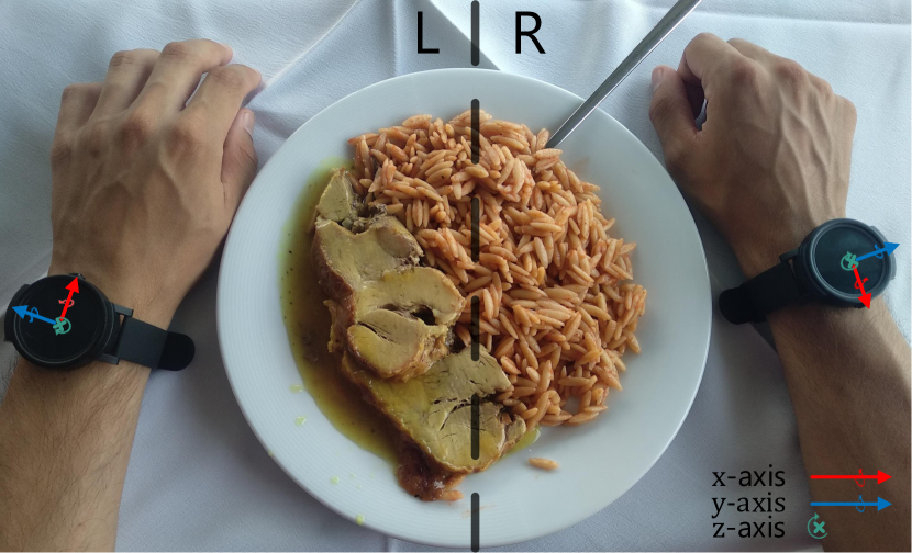
Figure 1: Figure depicting the orientation of the IMU sensors when the smartwatch is worn on either the left (L) or the right (R) hand of a participant. The figure also illustrates the need for adjusting the orientation of the accelerometer’s $x$ and gyroscope’s $y$ and $z$ axes in a way that when a hand moves then the movements of the opposing hand are reflected as if a mirror was placed on the dotted line. In all cases, the direction of the gyroscope’s axes is given by the right hand rule.

III-A2 Smoothing & gravity removal

To deal with the small fluctuations introduced by the sensors’ hardware we individually convolve each of the $3$D accelerometer and gyroscope streams with a moving average filter. After experimenting with different filter lengths we selected a length of $l_{ma}=25$ (considering a sampling frequency $f_{s}=100$ Hz) as it produced satisfactory results with minimal distortion. Each tap weight of the moving average filter was set to $1/25$.

Furthermore, since the accelerometer sensor captures the acceleration caused due to the Earth’s gravitational field in addition to the voluntary wrist movements, the final preprocessing step is to attenuate the Earth component. We achieve this by individually convolving the $\mathbf{a}_{x}$, $\mathbf{a}_{y}$ and $\mathbf{a}_{z}$ components of $\mathbf{R}$ with a high-pass finite impulse response (FIR) filter. The filter’s cutoff frequency $f_{c}$ and length of the tap delay line $l_{hp}$, were set to $1$ Hz and $512$ samples respectively.

III-B End-to-end network architecture

The proposed end-to-end architecture is comprised of two parts, the first one being the convolutional and the second the recurrent. The convolutional part has a depth of three $1$D convolutional layers with the first two being followed by max pooling operations that decimate the activations of the previous layer by a factor of $2$. The number of filters used in each convolutional layer increases as the depth increases. Specifically, we used $32$, $64$ and $128$ as the number of filters in each of the three convolutional layers. The filter lengths for each layer were selected to be $5$, $3$ and $3$ samples respectively; or $\frac{5}{fs}$, $\frac{3}{fs/2}$ and $\frac{3}{fs/4}$ secs due to the intermediate max pooling operations. All convolutional layers use the Rectified Linear Unit (ReLU) as the non-linearity for their activations, defined as $\rho(x)=\max(0,x)$.

Overall, the convolutional part of our network is inspired by the popular VGG [38] architecture for image classification; essentially increasing the number of filters in the convolutional layers after each max pooling application while keeping the same kernel sizes. Contrary to VGG, however, our architecture uses one convolution layer before max pooling instead of using pairs of convolution layers in-between max pooling layers. This helps in keeping the number of model parameters low.

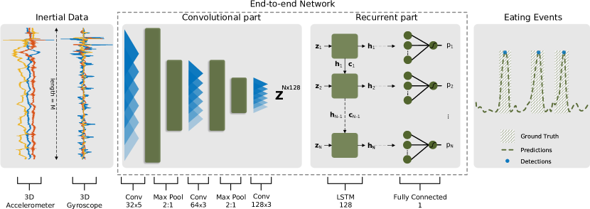
Figure 2: Overall pipeline of the in-meal bite detection approach. From left to right, the preprocessed inertial signals ($3$D acceleration and orientation velocity) of length $M$ that are captured during the meal are forwarded to the end-to-end network. The network processes the $M\times 6$ data, (essentially $\mathbf{R}$ from Section III-A), and outputs the $N$-dimensional bite probability vector $\mathbf{p}$, where $N=M/4$ due to the two max pooling operations. Variable $\mathbf{Z}$ with dimensions $N\times 128$ represents the intermediate output of the convolutional part of the end-to-end network while $h_{i}$ and $c_{i}$ represent the $i$-th output and cell state of the LSTM block.

The recurrent part consists of a single LSTM layer with $128$ hidden cells. We used the hard sigmoid function, defined as $\sigma_{h}(x)=\max(0,\min(1,0.2\cdot x+0.5))$, as the activation of the LSTM’s recurrent steps. During training the output of the network is obtained by propagating the final $128$-dimensional output of the LSTM layer to a fully connected layer with a single neuron and the sigmoid function as the activation, defined as $\sigma(x)=(1+e^{-x})^{-1}$. The total number of learnable parameters for the proposed network is $163,617$.

On the other hand, during inference we modified the LSTM layer to provide all intermediate outputs to the fully connected layer and subsequently the fully connected layer to provide an output $p$ for all intermediate outputs of the LSTM layer. In more detail, given a $M\times 6$ meal recording $\mathbf{R}$, the convolutional part of the inference network generates the $N\times 128$ internal variable $\mathbf{Z}$, with $N=M/4$ due to the two max pooling operations that decimate the activations by a factor of $2$ each. Subsequently, the recurrent part of the network (i.e. the LSTM layer) processes $\mathbf{Z}$ to produce the final $N\times 1$ prediction vector $\mathbf{p}$. Figure 2 depicts the architecture of the inference network as part of the in-meal bite detection pipeline.

III-C Training the network

For training examples, we used a sliding window of length $w_{l}$ and step $w_{s}$ to extract data frames from all meals in the training set. As a result, we obtain the set $\mathcal{X}=\{\mathbf{X}_{1},\mathbf{X}_{2},\cdots\}$, that contains the training examples, $\mathbf{X}_{i}$ each with dimensions $w_{l}\times 6$, from all meals. The process of extracting training samples continues by pairing each $\mathbf{X}_{i}$ with a label $y_{i}$. A label $y_{i}$ is positive when the end of the sliding window is within a distance ($\pm\epsilon$) from the end of a intake cycle event and negative for every other case. In the evaluation section (Section V-A) we present two different approaches for assigning values to $y_{i}$ depending on the available ground truth data. It should also be noted that during training the internal variable $\mathbf{Z}$ has dimensions $\frac{w_{l}}{4}\times 128$.

We also augmented the training set by artificially changing the orientation of the smartwatch on the wrist. In more detail, each example in the minibatch has a $50\%$ chance to be selected for transformation. If the example is selected then two random numbers, $\hat{\theta}_{x}$ and $\hat{\theta}_{z}$, are drawn from a normal distribution with mean and standard deviation equal to $0$ and $10$ respectively.

Then based on $\hat{\theta}_{x}$ and $\hat{\theta}_{z}$ we create two $3\times 3$ rotation matrices, namely $\mathbf{Q}_{x}(\hat{\theta}_{x})$ and $\mathbf{Q}_{z}(\hat{\theta}_{z})$ that correspond to rotation around the $x$ and $z$ axes, respectively. The final transformation $\mathbf{Q}$ is randomly chosen to be one of the following: i) $\mathbf{Q}_{x}(\hat{\theta}_{x})$, ii) $\mathbf{Q}_{z}(\hat{\theta}_{z})$, iii) $\mathbf{Q}_{x}(\hat{\theta}_{x})\cdot\mathbf{Q}_{z}(\hat{\theta}_{z})$ or iv) $\mathbf{Q}_{z}(\hat{\theta}_{z})\cdot\mathbf{Q}_{x}(\hat{\theta}_{x})$. The transformation is then applied to the chosen $i$-th training example $\mathbf{X}_{i}$ in the batch as:

$$\mathbf{X}^{\prime}_{i}=\left(\left[\begin{array}[]{@{\,} c|c @{\,}}\mathbf{Q}&\mathbf{0}_{3\times 3}\\ \hline\cr\mathbf{0}_{3\times 3}&\mathbf{Q}\\ \end{array}\right]\cdot\mathbf{X}_{i}^{\top}\right)^{\top}$$ (2)

Where $\mathbf{0}_{3\times 3}$ is used to represent a $3\times 3$ matrix of zeros. We selected not to perform any augmentation by rotating the $\mathbf{X}_{i}$ samples around the $y$ axis (i.e. by $\mathbf{Q}_{y}(\hat{\theta}_{y})$) as such rotation of the smartwatch on the wrist is not physically feasible. Applying such transformations allows us to mimic different positions ($\pm 10^{\circ}$) of the user’s smartwatch around the wrist. This allows us to introduce variability in the examples provided to the network during training.

During training the network minimizes the binary cross entropy loss,

$$\mathcal{{L}}=-\sum\limits_{i\in K}\Big{(}\hat{y}_{i}\log(\hat{p}_{i})-(1-\hat{y}_{i})\log(1-\hat{p}_{i})\Big{)}$$ (3)

where $\hat{y}\in\{-1,+1\}$ is the target, $\hat{p}_{i}$ is the network’s prediction for the $i$-th sequence in a mini-batch that contains $K$ examples. We also applied a $50\%$ dropout chance to the inputs of the fully connected layer as a form of regularization in order to avoid overfitting during training [39]. Finally, the network is trained using the RMSProp optimizer with a learning rate of $10^{-3}$ and a batch size of $128$ samples. Each batch contained an equal number of positive and negative training examples to avoid bias. After inspecting the learning curves regarding the training accuracy and cross entropy loss on the training set we observed only a marginal improvement after the $5$th epoch; therefore, we selected $5$ as the number of epochs for training the network.

III-D Bite detection

By processing an $M\times 6$ recording $\mathbf{R}$ that contains the preprocessed inertial observations, the inference end-to-end network outputs the $N$-length prediction series $\mathbf{p}$, with $N=M/4$ due to the max pooling operations (Section III-B). We perform bite detection by initially replacing with zeros the elements of $\mathbf{p}$ that are lower than a probability threshold $\lambda_{p}$. Next, by performing a local maxima search, with a minimum distance between two consecutive peaks set at $2$ seconds, on the thresholded series $\mathbf{p}$ we obtain the set of detected bites $\mathcal{B}=\{b_{1},\ldots,b_{L}\}$. Each $b_{i}$ element is essentially the timestamp that corresponds to the $i$-th peak.

Experimenting with a small part of the FIC dataset led us to select $0.89$ for the $\lambda_{p}$ threshold, as this value yielded the highest F$1$ score ($0.932$). This set included $4$ out of the $21$ available meals (approximately $19.04\%$), selected at random, and $319$ ground truth bites out of the total $1,332$ (approximately $23.94\%$).

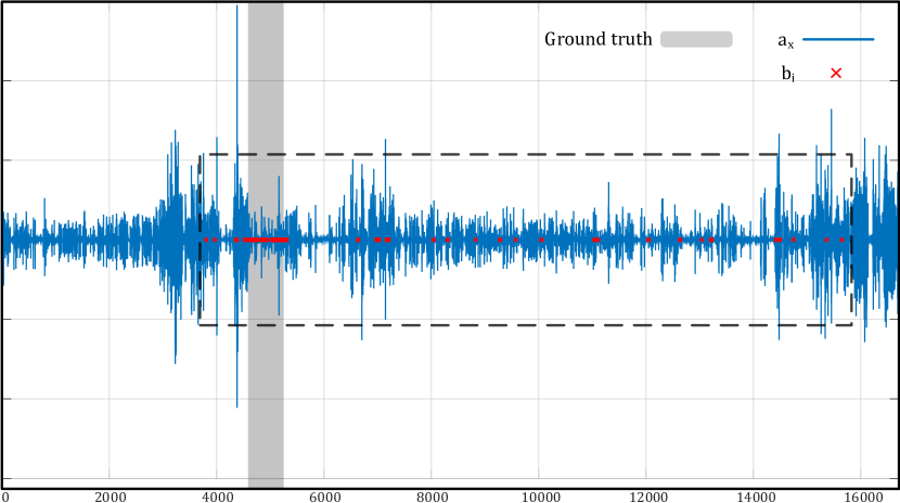
(a)

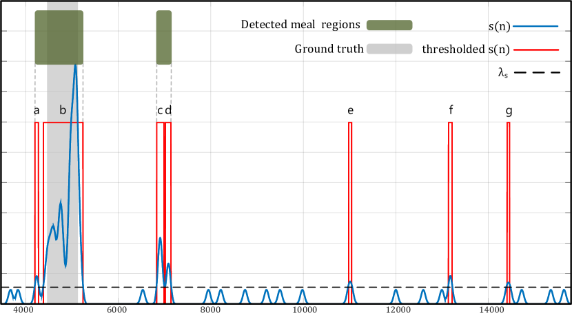
(b)

Figure 3: Example estimation of meal end-points. In both sub-figures the ground truth is depicted with the shaded background and the horizontal axis represents the time in seconds. Specifically, sub-figure a) shows the $\mathbf{a}_{x}$ axis of the accelerometer sensor and each red $\times$ symbol represents a bite detection $b_{i}$. Sub-figure b) focuses on the area of a) that is marked with the dotted line. It depicts the smoothed series $s(n)$ and how thresholding it by using $\lambda_{s}$ as a cutoff point we obtain the candidate meal intervals denoted with a, b, c, d, e, f and g. By iteratively merging nearby intervals and subsequently rejecting short meals, we estimate the final meal regions. In this specific example, intervals e, f and g where rejected while a and b as well as c and d were respectively merged and formed the two final meal estimates (depicted with green background).

IV In-the-wild meal detection

The term in-the-wild is usually used to describe the unconstrained nature of capturing conditions. In the context of this work, in-the-wild meals are meals that are typically found in long IMU recordings (significantly longer than the recordings used in Section III) obtained by participants during their every day life activities. In this section we present a method for effectively detecting the start and end time-points of in-the-wild meals using the trained end-to-end network from Section III coupled with signal processing algorithms.

IV-A End point detection algorithm

Given the $M\times 6$ observation matrix $\mathbf{R}$ that represents an in-the-wild recording and the trained end-to-end network, the first step is to obtain the set of detected bites $\mathcal{B}$ with cardinality $|\mathcal{B}|=L$. The next step is to construct the timeseries $s(n)$ with $n=1,\ldots,N$, that spans the entire duration of the recording and is equal to one only at the moments where a bite is detected and zero everywhere else. Formally:

$$s(n)=\begin{cases}1\text{,}&\text{if }n=b\cdot\frac{f_{s}}{4}\quad\forall\;b\in\mathcal{B}\\ 0\text{,}&\text{otherwise}\end{cases}$$ (4)

The timeseries $s(n)$ is then convolved with a Gaussian filter of length and standard deviation equal to $\frac{f_{s}\cdot 240}{4}$ and $\frac{f_{s}\cdot 45}{4}$ samples. The latter is important as it smooths $s(n)$ and closes the gaps between groups of bites that are close to each other, similar to a morphological closing operation, which is a phenomenon present in long meals.

We continue by replacing with zeros the elements of $s(n)$ that are below a threshold $\lambda_{\mathbf{s}}$ and with ones the elements that are above it; thus creating contiguous regions of fixed magnitude. We selected threshold $\lambda_{\mathbf{s}}$ to be equal to $5\times 10^{-4}$. The selected $\lambda_{\mathbf{s}}$ value is high enough to reject single, isolated, peaked in the smoothed $s(n)$ series. That simple thresholding scheme acts as a way of filtering out sparse, false positive detections that may appear throughout the day.

In order to extract the left-most and right-most edges of the contiguous regions found in $s(n)$ we first convolve the thresholded series $s(n)$ with an $1$D edge detector (or differentiation filter) $\mathbf{h}$ with a sidelobe length equal to $f_{s}/4$ samples, constructed as: $\mathbf{h}=[1,2,\ldots,\frac{f_{s}}{4},0,-\frac{f_{s}}{4},\ldots,-2,-1]$. The result of this process is the series $d(n)$ of length $N$. The final edges of the regions in $s(n)$ are obtained by performing a local maxima search in $|d(n)|$.

The first crude estimate of meal end-points is obtained by pairing the consecutive peaks found in $|d(n)|$ without overlapping between pairs, i.e. the first with the second, the third with the forth, etc. The outcome is the set of intervals $\mathcal{Q}=\{q_{1},\ldots,q_{V}\}$ where each $q_{i}=[t^{l}_{i},t^{r}_{i}]$ with $i=1,\ldots,V$, contains the timestamps of the left-most ($t^{l}_{i}$) and right-most ($t^{r}_{i}$) edges of the meal estimates. Next, we iteretively merge $q_{i}$ intervals that are within $180$ seconds of each other. We selected the merge threshold to be equal to $180$ as it adequately merged nearby meal regions and has marginal effect in the performance of the approach. Finally, all $q_{i}$ intervals with duration less that $180$ seconds are rejected. Figure 3 depicts the steps of the meal detection process.

V Experiments & Evaluation

V-A Datasets

In our experiments we make use of three datasets, namely FIC, FreeFIC and FreeFIC held-out. All datasets contain the triaxial acceleration and orientation velocity ($6$ DoF) signals originating from a commercial smartwatch. However, the FIC dataset differs from the other two regarding the context and the duration of the recordings. More specifically, recordings in FIC focus on in-meal behavior and therefore only contain meals, i.e. the recordings start and end when a meal starts and ends. On the other hand, FreeFIC and FreeFIC held-out recordings are significantly longer in duration (average FIC recording duration is $703$ seconds as opposed to $17,398$ seconds in FreeFIC and $21,234$ seconds in FreeFIC held-out) as they aim to detect eating episodes among the every day life activities of participants. Details on the datasets are as follows.

V-A1 The FIC dataset

FIC includes the inertial data from $21$ meal sessions belonging to $12$ unique subjects, recorded in the restaurant of Aristotle university of Thessaloniki. We used the Microsoft Band $2^{\text{TM}}$ for capturing ten out of the twenty-one meals and the Sony Smartwatch $2^{\text{TM}}$ for the rest.

Prior to each meal recording, a GoPro${}^{\text{TM}}$ Hero $5$ camera was already set to the participant’s table. The camera was mounted on a small $23$ cm in height tripod with the ability to capture the participants torso, face and food tray simultaneously. We used the video streams to annotate the start and end moments of each food intake cycle (i.e. bite) event that would serve as ground truth. No special instructions were given to the subjects, other than clapping their hands once before starting their meal and once after they were done. This is important since the clapping motion has a very distinctive footprint on the accelerometer signal (especially in the magnitude series that for a specific moment $m$ is defined as $m_{a}(m)=\sqrt{(a_{x}^{2}(m)+a_{y}^{2}(m)+a_{z}^{2}(m))}$) which enables the synchronization between the inertial data and the video stream. The participants were free to select the starter, salad, main and desert of their preference, thus creating a diverse set of food types such as, but not limited to, different kinds of meat or fish (such as chicken legs, lamb, pork, sea bass), different kinds of garnish (such as potatoes or rice), pasta, cooked vegetables (such as green beans or peas), soups and various types of salads (such as Greek-style salad, cauliflower or cabbage). Finally, FIC dataset does not contain liquid intake instances or eating without the fork, spoon and knife.

Given the video stream and inertial data for a meal we can create each meal’s label series $\mathbf{y}$.

$$y_{i}=\begin{cases}+1\text{,}&\text{if }t^{gt}_{j}-\epsilon\leq t^{y}_{i}\leq t^{gt}_{j}+\epsilon\\ -1\text{,}&\text{otherwise}\end{cases}$$ (5)

Where $y_{i}$ is the binary label associated with the $i$-th windowed data frame $\mathbf{X}_{i}$ (Section III-C), $t^{gt}_{j}$ represents the timestamp at the end of the $j$-th bite event and $t^{y}_{i}$ is the timestamp associated with $y_{i}$. In our experiments we set $\epsilon$ equal to $0.1$ seconds. Figure 4 a) depicts the labeling process for recordings in FIC. Table I provides the statistics for the FIC dataset.

Sliding window parameters $w_{l}$ and $w_{s}$ for extracting training data from the FIC dataset (Section III-C) were set to $5\cdot f_{s}$ and $0.05\cdot f_{s}$ samples, or $5$ and $0.05$ seconds respectively. We selected this value for $w_{l}$ as this window length approximates the mean food intake cycle duration in our dataset (Table I).

TABLE I: FIC dataset statistics

	Meal sessions	Food Intake Cycles
#	$21$	$1,332$
Mean (sec)	$703.56$	$4.52$
Std (sec)	$186.18$	$3.22$
Median (sec)	$717.88$	$3.55$
Total (sec)	$14,774.80$	$6,023.07$
Total (hours)	$4.10$	$1.67$
Participants	$12$
Ratio total/bites	$2.4$

V-A2 The FreeFIC dataset

FreeFIC includes $16$ in-the-wild sessions that belong to $6$ unique subjects. Four out of the six subjects in FreeFIC also participated in FIC. Participants were instructed to wear the smartwatch to the hand of their preference well ahead before any meal and continue to wear it throughout the day until the battery is depleted. We used the Huawei Watch $2^{\text{TM}}$ for $6$ out of the $16$ recordings and the Mobvoi TicWatch${}^{\text{TM}}$ for the rest. Similar to the FIC dataset, FreeFIC only contains recordings were the subjects consumed their meals using the fork and/or the spoon. In addition, we followed a self-report labeling model, meaning that the ground truth is provided from the participant by documenting the start and end moments of their meals to the best of their abilities as well as the hand they wear the smartwatch on.

Using the self-reports and the inertial data we can construct the label series $\mathbf{y}$. More formally:

$$y_{i}=\begin{cases}N/A\text{,}&\text{if }t^{s}_{j}\leq t^{y}_{i}\leq t^{e}_{j}\\ -1\text{,}&\text{otherwise}\end{cases}$$ (6)

Where $t^{s}_{j}$ and $t^{e}_{j}$ represent the start and end timestamps of the $j$-th meal in a free-living recording. Variables $y_{i}$ and $t^{y}_{i}$ are the same as in FIC. We use the label characterization Not Applicable (N/A) to signify that we cannot consider this label either as positive or as negative due to the high uncertainty of when the subject is performing a bite during a meal. Figure 4 b) depicts the labeling process for recordings in FreeFIC. Detailed statistics about FreeFIC are provided in Table II.

For the extraction of training samples from FreeFIC we used the same sliding window length $w_{l}$ but significantly increased the step $w_{s}$, from $0.05$ to $1$ sec. The reason behind the $\times 20$ increase is to avoid oversegmenting the significantly longer FreeFIC recordings, which can solely yield negative training examples.

TABLE II: FreeFIC dataset statistics

	In-the-wild sessions	Meals
#	$16$	$17$
Mean (sec)	$17,398$	$1,148$
Std (sec)	$4,884$	$502$
Median (sec)	$16,489$	$1,065$
Total (sec)	$278,378$	$19,520$
Total (hours)	$77.32$	$5.42$
Participants	$6$
Ratio total/meal	$14.2$

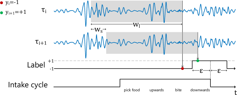
(a)

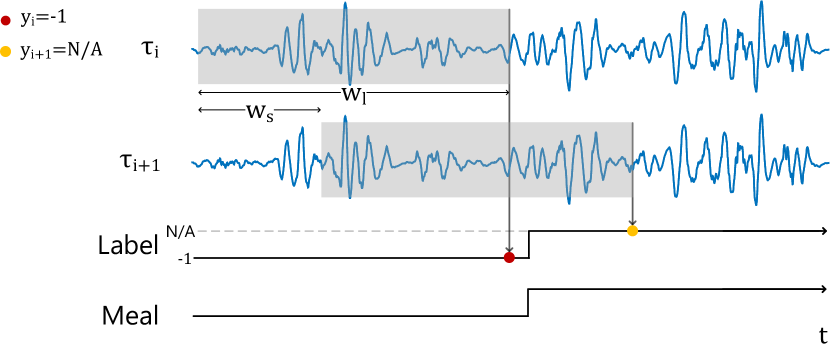
(b)

Figure 4: Example label extraction when $\mathbf{R}$ represents a) a meal recording or b) a free-living recording including one or more meals. Both subfigures depict the labeling process of two consecutive sliding windows at moments $\tau_{i}$ and $\tau_{i+1}$. The sliding window is illustrated by the shaded background while $w_{l}$ and $w_{s}$ represent it’s length and step. In the lower part of the subfigure a), for every moment $t$ the label signal is positive at the end of a food intake cycle ($\pm\epsilon$) and negative everywhere else. On the other hand for subfigure b), the label signal is negative everywhere except during the meals where it is not applicable or N/A. In both cases the label assigned to each window corresponds to the label at it’s right edge. For subfigure a), the window at $\tau_{i}$ is assigned a negative label while the window at $\tau_{i+1}$ a positive. Accordingly for subfigure b), the window at $\tau_{i}$ is also assigned a negative while the window at $\tau_{i+1}$ a N/A label.

V-A3 The FreeFIC held-out dataset

The FreeFIC held-out dataset includes $6$ in-the-wild sessions that belong to $6$ new unique subjects (one recording per participant). All recordings were captured using the Mobvoi TicWatch${}^{\text{TM}}$ smartwatch. The collection protocol and instructions provided to the participants were the same as the FreeFIC dataset (Section V-A2. However, in contrast to FreeFIC, no training examples were extracted from this held-out set. The FreeFIC held-out dataset was collected solely for testing purposes. It should also be emphasized that there is no overlap between the subjects in this held-out set and the FreeFIC/FIC datasets. Detailed statistics about FreeFIC held-out are presented in Table III.

TABLE III: FreeFIC held-out dataset statistics

	In-the-wild sessions	Meals
#	$6$	$6$
Mean (sec)	$21,234$	$960$
Std (sec)	$1,843$	$103$
Median (sec)	$21,876$	$960$
Total (sec)	$127,409$	$5,760$
Total (hours)	$35.39$	$1.6$
Participants	$6$
Ratio total/meal	$22.1$

V-B Experiments & evaluation methodology

V-B1 Food intake cycle detection experiments - EXI

The first series of experiments deals with measuring the performance of the end-to-end approach towards the detection of food intake cycles (i.e. bites) during the course of a meal. Specifically, we are interested in the cross-subject performance, or in other words how the method performs on meals that belong to unseen subjects. To achieve this, we used the positive and negative examples from the FIC dataset, $(\mathbf{X}_{i},y_{i})$ $\in$ FIC $\forall$ $i$ that satisfy $y_{i}=\pm 1$, as well as the negative examples from the FreeFIC dataset, $(\mathbf{X}_{i},y_{i})$ $\in$ FreeFIC $\forall$ $i$ that satisfy $y_{i}=-1$, to train our end-to-end network in a Leave-One-Subject-Out (LOSO) fashion. We discarded every $(\mathbf{X}_{i},y_{i})$ $\in$ FreeFIC pair where the respective $y_{i}$ had an N/A value (i.e. during a meal). At each LOSO step we iteretively exclude the recordings (both meal and in-the-wild sessions) of a single subject from the training process and use the meal sessions of the left-out subject to perform evaluation.

In addition, we extended EXI to include a series of experiments that aim to study the effects of synthetically augmenting the training set, according to the methodology presented in Section III-C, and how this can influence the food intake detection performance. The training and evaluation setup of this series of experiments is identical to EXI.

In all cases, we measure the performance of the bite detection algorithm by calculating the number of true positive (TP), false positive (FP) and false negative (FN) samples. It should be noted that the proposed in-meal bite detection evaluation scheme as well as the one proposed by Dong et al. in [11] cannot measure the number of True Negatives (TNs). Subsequently we can calculate the precision, recall and F$1$ metrics defined as $\text{Prec}=\frac{\text{TP}}{\text{TP}+\text{FP}}$, $\text{Rec}=\frac{\text{TP}}{\text{TP}+\text{FN}}$ and $\text{F1}=\frac{2\cdot\text{Prec}\cdot\text{Rec}}{\text{Prec}+\text{Rec}}$, respectively. In detail, given the set of detected bite moments, $\mathcal{B}$, and the set of in-meal ground truth intervals $\mathcal{G}^{m}=\{[t^{s}_{1},t^{e}_{1}],\ldots,[t^{s}_{N},t^{e}_{N}]\}$ calculation of the above metrics can be done in the following fashion:

• If a detected bite, $b_{i}\in[t^{s}_{j},t^{e}_{j}]$ exists for some $i$ and $j$ then we associate the $i$-th detection to the $j$-th ground truth interval:

  • If no other detection $b_{k}$, $k\neq i$ is associated with $j$, then it counts as a TP.

  • If a detection moment $b_{k}$ exists that is already associated with the $j$-th interval, then $b_{i}$ counts as a FP (i.e., at most one detected bite is associated with each ground truth interval).

• Detection moments that satisfy $b_{i}\not\in[t^{s}_{j},t^{e}_{j}]$ for all $j$ count as FPs as well.

• Any ground truth interval $[t^{s}_{j},t^{e}_{j}]$ that isn’t associated with a detection $b_{i}$ for any $i$, counts as a FN.

Figure 5 a) illustrates the proposed metric calculation scheme for EXI.

V-B2 In-the-wild meal detection experiment - EXII

The second series of experiments deals with measuring the performance of the meal detection method using in-the-wild recordings of FreeFIC (Table II). Experiment EXII is tightly linked with EXI in the sense that it makes use of the trained end-to-end networks $\mathbf{W}^{i}$ that were produced during the LOSO iterations of EXI, with $i=1,\ldots,S$ representing the identifier of the left-out subject out of the total $S$ subjects that participated in EXI, which for our experimental setup equals to $14$ (the number of unique subjects in the union of FIC and FreeFIC datasets). In more detail, for every subject $i$ in FreeFIC we use the trained end-to-end network $\mathbf{W}^{i}$ to produce the set of detected bites $\mathcal{B}^{i}_{k}$ for each of the $i$-th participant’s $k=1,\ldots,K$ total in-the-wild sessions. Subsequently each $\mathcal{B}^{i}_{k}$ is propagated to the meal detection algorithm (Section IV-A) in order to produce the final set of meal estimates $\mathcal{Q}^{i}_{k}$.

Similar to the evaluation of the bite detection approach, we can measure the effectiveness of the meal detection algorithm by exhaustively calculating the TP, FP, FN and TN metrics. Ability to measure TNs allows us to also calculate specificity and accuracy, defined as $\text{Spec}=\frac{\text{TN}}{\text{TN}+\text{FP}}$ and $\text{Acc}=\frac{\text{TP}+\text{TN}}{\text{TP}+\text{FN}+\text{FP}+\text{TN}}$. Motivated by [22], we opt to weight TP to TN at a ratio of $14.2$:$1$. This is due to the fact eating activities occupy a very small portion of time in free-living scenarios. The $14.2$ weighting ratio results from Table II, by dividing the total recording duration with the time spend during meals, specifically $77.32/5.42=14.2$. Applying the weighting factor to the accuracy formula leads us to the weighted accuracy (as in Section II-C of [22]) defined as:

$$\textrm{Acc}_{w}=\frac{\textrm{TP}\cdot 14.2+\textrm{TN}}{(\textrm{TP}+\textrm{FN})\cdot 14.2+\textrm{FP}+\textrm{TN}}$$ (7)

In order to measure TPs, FPs, TNs and FNs, we consider the discrete complete free-living timeline and that each point in time that corresponds to a $q_{i}$ interval (i.e. in-between $t^{l}_{i}$ and $t^{r}_{i}$) belongs to the positive class (i.e. meal) and every other point to the negative (i.e. non-meal). Moreover, we can also assess the meal detection effectiveness by calculating the overlap of the detected meal intervals against the real ones using the Jaccard Index metric, defined as $\mathcal{J}(\mathcal{Q},\mathcal{T})=\frac{|\mathcal{Q}\cap\mathcal{T}|}{|\mathcal{Q}\cup\mathcal{T}|}$, where $\mathcal{Q}$ and $\mathcal{T}$ are the estimated and true meal intervals, respectively. Figure 5 b) depicts an example of how we measure the effectiveness of the meal detection algorithm.

(a)

(b)

Figure 5: Proposed metric calculation schemes for measuring the effectiveness of the a) bite detection and b) meal detection algorithms.

V-B3 In-the-wild held-out meal detection experiment - EXIII

The third series of experiments also deals with the detection of meals using in-the-wild recordings. However, EXIII primarily focuses on supporting the outcomes of the LOSO experiments (EXII, Section V-B2) and evaluating the generalization ability of the presented approach. To this end, in EXIII we use the FIC and FreeFIC datasets (Sections V-A1 and V-A2) as training sets and the FreeFIC held-out dataset (Section V-A3) as the test set (no overlapping subjects between the FIC/FreeFIC and the FreeFIC held-out datasets).

In more detail, in EXIII we use all available data from FIC and FreeFIC to train a single end-to-end network $\mathbf{W}$. It should be emphasized that network $\mathbf{W}$ was built before collecting the FreeFIC held-out dataset (Section V-A3). The network is then used to produce the set of detected bites for each one of the $6$ in-the-wild sessions belonging to the $6$ subjects participating in the FreeFIC held-out set. Finally, each set of detected bites is propagated to the meal detection algorithm in order to obtain the final set of of meal estimates.

Performance metrics are extracted in the same fashion as in EXII, with the exception of the accuracy weighting factor which is calculated from Table III as $35.39/1.6=22.1$.

V-B4 In-the-wild meal detection using external dataset experiment - EXIV

Similar to EXII and EXIII (Sections V-B2 and V-B3), the fourth series of experiments (EXIV) also deals with the detection of meals using in-the-wild recordings. The experiments performed in this section aim to to further validate the proposed method’s ability to generalize on previously unseen data, using a publicly available external dataset with similar information. In more detail, we opted to use the ACE Free-living dataset presented by Mirtchouk et al. in [27].

The ACE Free-living dataset consists of two sub-datasets, ACE-FL and ACE-E, and contains a total of $25$ in-the-wild recordings from $11$ subjects ($10$ recordings belonging to $5$ subjects from ACE-FL and $15$ recordings belonging to $6$ subjects from ACE-E). Each recording in ACE Free-living contains: 1) $9$ DoF IMU data from two commercial smartwatches, 2) $9$ DoF IMU data from a Google Glass (only for ACE-FL), and 3) audio information from an earbud with internal and external microphones. All IMU data were collected at a rate of $15$ Hz. Annotation includes the start and end moments of all eating activities, the meal type (meal, snack or drink) and the items that were consumed. Participants could eat their food with or without utensils as well as using either, or even both, hands.

In the scope of EXIV, the ACE Free-living dataset differs from the FreeFIC/FreeFIC held-out datasets in terms of: 1) the IMU sampling frequency ($15$ against $100$ Hz), 2) the number of smartwatches used ($2$ against $1$), 3) additional meal types (meals, snacks and drinks against just meals) and 4) usage of utensils (fork, spoon and knife) during meals since the subjects in ACE Free-living can also eat using their bare hands.

For the experiments performed in this section we used the $6$ DoF IMU data (3D acceleration and orientation velocity) originating from both hands (formulated as the $M\times 6$ observation matrices $\mathbf{R}_{l}$ and $\mathbf{R}_{r}$ for the left and right hand, respectively), after appropriately upsampling to the frequency that is compatible with our approach ($f_{s}=100$ Hz). Furthermore, the EXIV series of experiments is performed in a similar fashion as EXIII (Section V-B3). Specifically, we use all available data from the FIC and FreeFIC datasets to train a single end-to-end network $\mathbf{W}$ and use ACE Free-living (all data from both ACE-FL and ACE-E) as the held-out test set. By independently processing $\mathbf{R}_{l}$ (mirrored appropriately using Equation 1) and $\mathbf{R}_{r}$ using $\mathbf{W}$, we obtain the two sets of detected bites $\mathcal{B}_{l}$ and $\mathcal{B}_{r}$. The final meal estimates are obtained by forwarding the combined set of bite detections $\mathcal{B}_{lr}=\mathcal{B}_{l}\cup\mathcal{B}_{r}$ to the meal detection algorithm. In our experiments we evaluate how well our approach generalizes on the unseen ACE Free-living dataset using only the annotated meals as the positive eating activities (snacks and drinks are considered negative). We also performed an experiment using the annotated meals and snacks as positive eating activities (drinks are considered negative); however, it is expected a priori to achieve reduced accuracy since the snacks category does not always have the meal structure that we assume in our analysis.

V-C Results & discussion

Regarding the EXI series of experiments (Section V-B1, we compare the performance of the proposed algorithm against four state-of-the art methods in the same datasets. The first one is the work of Zhang et al. [9], the second one is the work of Dong et al. [11] and the two other works [10] and [34] belong to our group. A synopsis of the aforementioned works has been provided in Section II. One fundamental difference in the core of those methods is dependency on micromovements. Specifically, the works of [10, 34, 9] rely on knowledge of micromovements while the work of [11] and the method proposed in this paper are micromovement-agnostic.

Table IV presents the results of EXI, using: i) the evaluation scheme explained in Section V-B1 (also depicted in Figure 5 a) and ii) the more relaxed evaluation scheme of [11]. Evaluation results indicate that the proposed approach outperforms all other methods, both micromovement-based and micromovement-agnostic, by achieving an F$1$ score of $0.928$ using the proposed evaluation scheme. Our previous micromovement-based approach presented in [10] achieves the second highest performance with an F$1$ score of $0.913$ under the same scheme. When switching to the less strict evaluation scheme of Dong et al. [11] an overall increase to F$1$ can be observed across all experiments. In addition to the F$1$ increase, the performance-wise ranking of the compared methods is preserved except the first two places where the method of [10] marginally outperforms the proposed one with an F$1$ score of $0.929$ over $0.928$.

Table V shows the effects of synthetically augmenting the dataset during the training process of the proposed method regarding the intake cycle detection performance. Specifically, the best performance is obtained by allowing the training data to be rotated both around the $x$ (roll) and $z$ (yaw) axes, thus achieving an F$1$ score of $0.923$. Solely rotating the training data around the $x$ or the $z$ axis yield a score of $0.911$ and $0.919$, respectively. Overall, synthetically augmenting the dataset by rotating around $x$ and $z$ results into a considerable improvement over not using data augmentation at all which achieves the lowest performance of all four trials with an F$1$ score of $0.888$.

Regarding the first series of in-the-wild meal detection experiments (EXII, Section V-B2), we compare the proposed approach with the one presented by Dong et al. [22]. In contrast to our bite-based meal detection method that makes the hypothesis of the density of the detected bites being low outside the meal intervals, the core behind [22] is that before and after every meal a period of increased wrist motion energy is observed. At the same time the authors also assume that the wrist motion energy during the course of a meal tends to be reduced. The wrist motion formula is formally defined by the authors as:

$$E(i)=\frac{1}{W+1}\sum_{i=t-\frac{W}{2}}^{t+\frac{W}{2}}|a_{x}(i)|+|a_{y}(i)|+|a_{z}(i)|$$ (8)

where $a_{x}(i)$, $a_{y}(i)$ and $a_{z}(i)$ are the smoothed $x$, $y$ and $z$ channels of the accelerometer sensor and $W$ is the length of the sliding window over which the wrist motion energy is calculated for a single moment. We implemented the method of [22] and subsequently used a small subset of the in-the-wild recordings to tune: i) the length of the window size (W) and ii) the multiplication factor between the T$1$ and T$2$ thresholds, that affects the segmentation part of their method. Throughout our experiments, we used the complete feature set as suggested by the authors.

Furthermore, we compare our method with Density-Based Spatial Clustering of Applications with Noise (DBSCAN). The motivation behind using DBSCAN as a solution to the meal detection problem stems from the work of Zhang et al. [9] where the authors employ DBSCAN in order to detect the final bite moments using the density of bite decisions produced by their algorithm. In this experiment we transfer the application of DBSCAN from detecting eating moments to detecting meals found in the wild. We provide as input to DBSCAN the $\mathcal{B}_{k}^{i}$ set of bite timestamps, for the $k$-th session of the $i$-th subject, as computed by our proposed end-to-end network. In addition and to be on par with our proposed meal detection approach we parameterize DBSCAN accordingly by setting the maximum distance between samples (usually mentioned as the eps parameter) to $180$ seconds. To obtain the final meal estimates using DBSCAN we pair the two extreme points of each formed cluster.

The first half of Table VI summarizes the performance of all meal detection algorithms in a LOSO evaluation setting using the FreeFIC set. The results initially point out that the proposed approach outperforms all other methods by yielding an F$1$/weighted accuracy/Jaccard Index of $0.899$/$0.953$/$0.820$. In addition, both methods that use the distribution of the detected bites in order to perform meal detection exhibit increased performance.

One potential reason behind the difference between the results reported in [22] and the ones reported here is the nature of the sensing device (strapped phone on the wrist against smartwatch). In addition, the authors of both [22] and [36] report that the hypothesis of vigorous wrist movement before and after a meal can be population- and lifestyle-specific.

Experimental results from the second series of the in-the-wild meal detection experiments (EXIII, Section V-B3) support the results obtained from the LOSO experiments (EXII, Section V-B2. The second half of Table VI presents the performance of all meal detection algorithms using the FreeFIC held-out set as described in V-B3. Comparison between the first and second halves of Table VI reveal that the proposed approach achieves almost identical results with the ones obtain in EXII; specifically, an F$1$ score of $0.896$ ($0.899$ in EXII), a weighted accuracy of $0.964$ ($0.953$ in EXII), and a Jaccard Index of $0.821$ ($0.820$ in EXII). The similarity in the obtained results in the two in-the-wild datasets clearly indicates that the LOSO test error estimation of EXII is accurate and that the proposed method generalizes in previously unseen samples. This argument is further supported by the fact that the collection of the FreeFIC held-out set initiated after the completion of the LOSO experiments (EXII).

Finally, Table VII showcases the obtained in-the-wild meal detection results when using the external publicly-available dataset presented in [27] (EXIV, Section V-B4). More specifically, by using the inertial information from both hands, the proposed meal localization method achieves a weighted accuracy of $0.825$ when using only the meal sessions as positive periods. In addition, when using both the meals and snacks as positive periods, the proposed method yields a weighted accuracy of $0.788$. Results of this experiment on $15$ Hz sampling rate data of an external dataset further demonstrate the robustness of our method and it’s ability to generalize on previously unseen data. It should be emphasized that apart from upsampling the ACE IMU signals (from $15$ to $100$ Hz), this performance was achieved without retraining the method (or tuning any parameters) to the specific dataset.

TABLE IV: Bite detection performance results. The table contains the results of EXI using the evaluation scheme described in V-B1.The $\star$ symbol in the method proposed by Dong et al. is used to signify that parameter tuning was performed by optimization based on our proposed evaluation scheme (Figure 5 a). The numbers inside the parentheses represent the results obtained using the evaluation scheme proposed in [11].

Bite detection method	Micromovements (y/n)	TP	FP	FN	Prec	Rec	F1
Proposed	n	$1,231$ ($1,237$)	$102$ ($96$)	$101$ ($95$)	$.923$ ($.927$)	$.924$ ($.928$)	$\mathbf{.923}$ ($.928$)
Kyritsis et al. [10]	y	$1,241.8$ ($1,263.4$)	$144.5$ ($122.9$)	$90.2$ ($68.6$)	$.895$ ($.911$)	$.932$ ($.948$)	$.913$ ($\mathbf{.929}$)
Kyritsis et al. [34]	y	$1,221.5$ ($1,267.6$)	$228.4$ ($182.3$)	$110.5$ ($64.4$)	$.842$ ($.874$)	$.917$ ($.951$)	$.878$ ($.911$)
Zhang et al.[9]	y	$944$ ($1,102$)	$431$ ($233$)	$388$ ($230$)	$.686$ ($.825$)	$.708$ ($.827$)	$.697$($.826$)
Dong et al.[11]	n	$707$ ($1,190$)	$794$ ($311$)	$625$ ($142$)	$.471$ ($.792$)	$.530$ ($.893$)	$.499$ ($.840$)
Dong et al.[11] $\star$	n	$772$ ($1,214$)	$746$ ($304$)	$560$ ($118$)	$.508$ ($.799$)	$.579$ ($.911$)	$.541$ ($.851$)

TABLE V: Effects of proposed data augmentation scheme (Section III-C) applied during the training of the proposed end-to-end network regarding the in-meal bite detection performance.

Data augmentation method	TP	FP	FN	Precision	Recall	F1
None	$1,145$	$101$	$187$	$.918$	$.859$	$.888$
Around x axis (roll)	$1,215$	$120$	$117$	$.910$	$.912$	$.911$
Around z axis (yaw)	$1,210$	$91$	$122$	$.930$	$.908$	$.919$
Around x & z axes	$1,231$	$102$	$101$	$.923$	$.924$	$\mathbf{.923}$

TABLE VI: In-the-wild meal start/end point detection results. The table presents the results of experiments EXII (first half) and EXIII (second half) using the proposed meal detection approach, DBSCAN and the one presented in [22].

Experiment	Meal detection method	Prec	Rec	Spec	F1	Accuracy	Weighted Accuracy	$\mathcal{J}$ Index
EXII (LOSO)	Proposed	$.880$	$.919$	$.990$	$.899$	$.985$	$\mathbf{.953}$	$.820$
	DBSCAN	$.838$	$.895$	$.986$	$.865$	$.980$	$.939$	$.752$
	Dong et al. [22]	$.323$	$.525$	$.919$	$.400$	$.892$	$.545$	$.255$
EXIII (Held-out set)	Proposed	$.858$	$.937$	$.992$	$.896$	$.990$	$\mathbf{.964}$	$.821$
	DBSCAN	$.774$	$.779$	$.989$	$.776$	$.979$	$.882$	$.681$
	Dong et al. [22]	$.105$	$.697$	$.714$	$.182$	$.717$	$.182$	$.089$

TABLE VII: In-the-wild meal start/end point detection results obtained using the proposed method and the ACE Free-living dataset as the held-out test set (EXIV, Section V-B4). Accuracy is weighted using a factor of $15.12$ and $12.02$ for the first (meals only) and the second (meals & snacks) experiment, respectively.

Positive periods	Prec	Rec	Spec	F1	Accuracy	Weighted Accuracy	$\mathcal{J}$ Index
Meals only	$.397$	$.710$	$.934$	$.509$	$.921$	$.825$	$.346$
Meals & snacks	$.457$	$.633$	$.939$	$.531$	$.917$	$.788$	$.377$

VI Limitations

One of the limitations of the presented bite detection approach (Section III) is the unpredictable behavior of the algorithm when the participant performs drinking gestures or eats without using the fork or the spoon, e.g., using bare hands or a pair of chopsticks. This unpredictable behavior stems from the fact that such examples were not introduced appropriately to the network during training. For example, liquid intake episodes that appear outside of meals in the in-the-wild recordings of FreeFIC dataset are considered as negative samples. The presented work is focused on meals centered around the use of the fork and/or the spoon.

A limitation of our evaluation approach is the inability to measure the in-meal bite detection performance using the in-the-wild recordings of FreeFIC and FreeFIC held-out. Despite the promising in-meal bite detection results (EXI, first row of Table IV), the appearance of single, isolated, bite detections outside of meals in the in-the-wild recordings can be characterized as over-estimation. However, this is handled by the thresholding scheme proposed in Section IV-A. In addition, the collection protocol lacks obtaining information other than the timestamps of the start and end moments of the meals throughout the day. For example, in the work presented in [27] the participants also took pictures before eating their meals, thus allowing for more complex types of future analysis.

A technical limitation of the proposed approach is the ability to be executed in-real time. While to this day smartwatch processing capabilities remain low, modern smartphones have begun to offer on-chip AI support (e.g. the Huawei Ascend 910), which can provide real time performance in cases where the models are shallow. The proposed model consists of $160,000$ parameters which suggests that the real-time feedforwarding small batches of data to the mobile device is a realistic scenario. Another technical limitation regarding the recording of IMU signals throughout the day is the high battery consumption when capturing the gyroscope sensor. However, we have not explored methods for overcoming either of the two technical limitations yet. Instead, in this paper we investigate the feasibility of an automated and objective eating behavior monitoring approach where the collected signals are transmitted and are processed remotely.

VII Conclusions and future work

In this paper, a complete framework towards the in-the-wild modeling of eating behavior using the IMU signals from a commercial smartwatch has been presented. The proposed framework consists of two parts. Initially, we follow a representation learning approach that includes an end-to-end NN with both convolutional and recurrent layers to detect bite events. Next we use the distribution of detected bites throughout the day to temporally localize meals by detecting their start and end points, using signal processing algorithms.

Experimental results using $12$ subjects for the LOSO in-meal bite detection experiments (EXI) as well as $12$ subjects for the meal localization experiments ($6$ evaluated in a LOSO fashion in EXII and $6$ evaluated in a held-out fashion in EXIII, without overlap between the two populations) showcase the high potential of the proposed approach. In more detail, we initially perform LOSO evaluation using our publicly available FIC and FreeFIC datasets where the proposed framework outperforms other state-of-the-art methods found in the recent literature ($0.923$ F$1$ score for in-meal bite detection and $0.820$/$0.953$ Jaccard Index/weighted accuracy for the temporal localization of in-the-wild meals). In addition to the LOSO experiments, we also perform evaluation regarding the detection of meal start/end points using the FreeFIC held-out set where our proposed approach achieves similar results with the LOSO experiments ($0.821$/$0.964$ Jaccard Index/weighted accuracy). Finally, the proposed method’s ability to generalize on unseen data is further validated (by achieving $0.346$/$0.825$ Jaccard Index/weighted accuracy) by using an external publicly-available dataset that contains in-the-wild sessions. Overall, the results reported in V-C are promising and point out the potential of the framework towards monitoring and modeling eating behavior.

Future work includes increasing the size of the in-the-wild datasets by recruiting additional subjects as well as increasing the length of the recordings by solving the battery issue that arises when recording the accelerometer and gyroscope at a high sampling rate. Investigation of drinking and/or eating without utensils gestures is also one potential direction of the current work. Additionally, we plan to extend our work by including additional cues, e.g., visual, with the aim of further increasing the bite detection performance. Finally, in an ongoing study we attempt to correlate in-meal indicators that derive from bite detections, with bradykinesia and parkinsonian tremor using data from healthy controls, early and advanced Parkinson’s Disease (PD) patients.

References

- [1] W. H. Organization, Obesity: preventing and managing the global epidemic. World Health Organization, 2000, no. 894.
- [2] B. Caballero, “The Global Epidemic of Obesity: An Overview,” Epidemiologic Reviews, vol. 29, no. 1, pp. 1–5, 06 2007.
- [3] C.-C. Yang and Y.-L. Hsu, “A review of accelerometry-based wearable motion detectors for physical activity monitoring,” Sensors, 2010.
- [4] A. Bonomi and K. Westerterp, “Advances in physical activity monitoring and lifestyle interventions in obesity: a review,” International journal of obesity, vol. 36, no. 2, p. 167, 2012.
- [5] D. A. Schoeller, “How Accurate Is Self-Reported Dietary Energy Intake?” Nutrition Reviews, vol. 48, no. 10, pp. 373–379, 10 1990.
- [6] V. Papapanagiotou, C. Diou, I. Ioakimidis, P. Sodersten, and A. Delopoulos, “Automatic analysis of food intake and meal microstructure based on continuous weight measurements,” IEEE Journal of Biomedical and Health Informatics, pp. 1–1, 2018.
- [7] W. J. Korotitsch and R. O. Nelson-Gray, “An overview of self-monitoring research in assessment and treatment.” Psychological Assessment, vol. 11, no. 4, p. 415, 1999.
- [8] T. Vu et al., “Wearable food intake monitoring technologies: A comprehensive review,” Computers, vol. 6, no. 1, 2017.
- [9] S. Zhang et al., “Food watch: Detecting and characterizing eating episodes through feeding gestures,” ser. BodyNets ’16, 2016.
- [10] K. Kyritsis, C. Diou, and A. Delopoulos, “Modeling wrist micromovements to measure in-meal eating behavior from inertial sensor data,” IEEE Journal of Biomedical and Health Informatics, pp. 1–1, 2019.
- [11] Y. Dong et al., “A new method for measuring meal intake in humans via automated wrist motion tracking,” Applied psychophysiology and biofeedback, vol. 37, no. 3, 2012.
- [12] G. Mertes et al., “Measuring weight and location of individual bites using a sensor augmented smart plate,” in Engineering in Medicine and Biology Society (EMBC), 2018.
- [13] H. Kalantarian and M. Sarrafzadeh, “Audio-based detection and evaluation of eating behavior using the smartwatch platform,” Computers in Biology and Medicine, vol. 65, pp. 1 – 9, 2015.
- [14] S. Päßler, M. Wolff, and W.-J. Fischer, “Food intake monitoring: an acoustical approach to automated food intake activity detection and classification of consumed food,” Physiological Measurement, vol. 33, no. 6, pp. 1073–1093, may 2012.
- [15] M. M. Anthimopoulos et al., “A food recognition system for diabetic patients based on an optimized bag-of-features model,” IEEE Journal of Biomedical and Health Informatics, vol. 18, no. 4, 2014.
- [16] F. Zhu, M. Bosch, N. Khanna, C. J. Boushey, and E. J. Delp, “Multilevel segmentation for food classification in dietary assessment,” in 2011 7th International Symposium on Image and Signal Processing and Analysis (ISPA), Sept 2011, pp. 337–342.
- [17] Y. Kawano and K. Yanai, “Real-time mobile food recognition system,” in The IEEE Conference on Computer Vision and Pattern Recognition (CVPR) Workshops, June 2013.
- [18] F. Kong and J. Tan, “Dietcam: Automatic dietary assessment with mobile camera phones,” Pervasive and Mobile Computing, vol. 8, 2012.
- [19] V. Papapanagiotou, C. Diou, and A. Delopoulos, “Chewing detection from an in-ear microphone using convolutional neural networks,” in Engineering in Medicine and Biology Society (EMBC), July 2017.
- [20] S. Päßler and W. J. Fischer, “Acoustical method for objective food intake monitoring using a wearable sensor system,” in 2011 5th International Conference on Pervasive Computing Technologies for Healthcare (PervasiveHealth) and Workshops, May 2011, pp. 266–269.
- [21] E. Thomaz, I. Essa, and G. D. Abowd, “A practical approach for recognizing eating moments with wrist-mounted inertial sensing,” in Proceedings of the 2015 ACM International Joint Conference on Pervasive and Ubiquitous Computing. ACM, 2015.
- [22] Y. Dong et al., “Detecting periods of eating during free-living by tracking wrist motion,” IEEE Journal of Biomedical and Health Informatics, vol. 18, no. 4, pp. 1253–1260, July 2014.
- [23] D. Gomes and I. Sousa, “Real-time drink trigger detection in free-living conditions using inertial sensors,” Sensors, vol. 19, no. 9, 2019.
- [24] D. Ortega Anderez, A. Lotfi, and A. Pourabdollah, “Eating and drinking gesture spotting and recognition using a novel adaptive segmentation technique and a gesture discrepancy measure,” Expert Systems with Applications, 2019.
- [25] V. Papapanagiotou, C. Diou, L. Zhou, J. van den Boer, M. Mars, and A. Delopoulos, “A novel chewing detection system based on ppg, audio, and accelerometry,” IEEE Journal of Biomedical and Health Informatics, vol. 21, no. 3, pp. 607–618, May 2017.
- [26] Chongguang Bi et al., “Familylog: A mobile system for monitoring family mealtime activities,” in 2017 IEEE International Conference on Pervasive Computing and Communications (PerCom), 2017.
- [27] M. Mirtchouk et al., “Recognizing eating from body-worn sensors: combining free-living and laboratory data,” Proceedings of the ACM on Interactive, Mobile, Wearable and Ubiquitous Technologies, vol. 1, no. 3, 2017.
- [28] R. Zhang and O. Amft, “Monitoring chewing and eating in free-living using smart eyeglasses,” IEEE Journal of Biomedical and Health Informatics, vol. 22, no. 1, pp. 23–32, Jan 2018.
- [29] J. M. Fontana, M. Farooq, and E. Sazonov, “Automatic ingestion monitor: A novel wearable device for monitoring of ingestive behavior,” IEEE Transactions on Biomedical Engineering, vol. 61, no. 6, 2014.
- [30] M. Mirtchouk et al., “Automated estimation of food type from body-worn audio and motion sensors in free-living environments,” in Machine Learning for Healthcare Conference, 2019, pp. 641–662.
- [31] H. Heydarian et al., “Assessing eating behaviour using upper limb mounted motion sensors: A systematic review,” Nutrients, 2019.
- [32] Y. Shen, J. Salley, E. Muth, and A. Hoover, “Assessing the accuracy of a wrist motion tracking method for counting bites across demographic and food variables,” IEEE Journal of Biomedical and Health Informatics, vol. 21, no. 3, pp. 599–606, May 2017.
- [33] K. Kyritsis, C. Diou, and A. Delopoulos, “End-to-end learning for measuring in-meal eating behavior from a smartwatch,” in Engineering in Medicine and Biology Society (EMBC), July 2018.
- [34] K. Kyritsis, C. Diou, and A. Delopoulos, “Food intake detection from inertial sensors using LSTM networks,” in International Conference on Image Analysis and Processing. Springer, 2017, pp. 411–418.
- [35] M. Farooq and E. Sazonov, “Detection of chewing from piezoelectric film sensor signals using ensemble classifiers,” in Engineering in Medicine and Biology Society (EMBC), Aug 2016, pp. 4929–4932.
- [36] S. Sharma et al., “Automatic detection of periods of eating using wrist motion tracking,” in First International Conference on Connected Health: Applications, Systems and Engineering Technologies, 2016.
- [37] K. Kyritsis, C. Diou, and A. Delopoulos, “Detecting meals in the wild using the inertial data of a typical smartwatch,” in Engineering in Medicine and Biology Society (EMBC), 2019.
- [38] K. Simonyan and A. Zisserman, “Very deep convolutional networks for large-scale image recognition,” CoRR, vol. abs/1409.1556, 2014.
- [39] N. Srivastava et al., “Dropout: A simple way to prevent neural networks from overfitting,” J. Mach. Learn. Res., vol. 15, no. 1, 2014.