Turbulent radiative diffusion and turbulent Newtonian cooling

Abstract

Radiation transport plays important roles in stellar atmospheres, but the effects of turbulence are being obscured by other effects such as stratification. Using radiative hydrodynamic simulations of forced turbulence, we determine the decay rates of sinusoidal large-scale temperature perturbations of different wavenumbers in the optically thick and thin regimes. Increasing the wavenumber increases the rate of decay in both regimes, but this effect is much weaker than for the usual turbulent diffusion of passive scalars, where the increase is quadratic for small wavenumbers. The turbulent decay is well described by an enhanced Newtonian cooling process in the optically thin limit, which is found to show a weak increase proportional to the square root of the wavenumber. In the optically thick limit, the increase in turbulent decay is somewhat steeper for wavenumbers below the energy-carrying wavenumber of the turbulence, but levels off toward larger wavenumbers. In the presence of turbulence, the typical cooling time is comparable to the turbulent turnover time. We observe that the temperature takes a long time to reach equilibrium in both the optically thin and thick cases, but in the former, the temperature retains smaller scale structures for longer.

I Introduction

An important property of turbulence is the mixing of fields that are advected by the flow. The simplest example is that of a passive scalar, a quantity that does not backreact on the flow. The magnetic field is another popular example, because for weak field strengths, it can be treated as a passive vector field, making the mathematics more straightforward compared to the fully nonlinear case. Even the flow itself is mixed by the turbulence, which is a much harder problem. This leads to turbulent viscosity, which acts as an enhanced molecular viscosity, although there can be additional important effects if the turbulence is anisotropic. Examples of additional effects occur in stratified flows in the presence of rotation. Such flows can become differentially rotating through what is called the $\Lambda$ effect Rue80 . It is a nondiffusive effect, analogous to the $\alpha$ effect in mean-field dynamo theory Mof78 ; KR80 . These nondiffusive effects have led to significant attention in astrophysics. Scalars, active or passive, have received comparatively less attention, because nondiffusive effects are generally less profound, but see Rädler et al. Rädler et al. (2011) for the slow-down of turbulent diffusion in certain compressive flows.

Prandtl suggested that turbulence has a smoothing effect—just like molecular diffusion. The molecular diffusion coefficient is generally proportional to the product of the typical velocity of the molecules, which is essentially the sound speed, and the typical mean-free path between collisions. Prandtl generalized this to turbulence by using the product of the typical velocity of the turbulent eddies and their correlation length, which he referred to as the mixing length. Important applications of turbulent mixing in astrophysics include turbulent convection in the Sun and stars, as well as mixing of chemicals in the Galaxy. The latter is a typical case of a passive scalar, while in the former case, the quantity that is being mixed is the specific entropy, which is an active scalar, because it affects the density in the momentum equation and can lead to buoyancy. Furthermore, the resulting turbulent diffusion is an enhancement not of molecular diffusion, but of photon diffusion, which is also referred to as radiative diffusion.

Radiative diffusion comes in two different forms: optically thick and optically thin. Optically thick is the usual case, where the mean-free path of photons is short compared to the typical scales of the flow. Optically thin, by contrast, means that the photons can propagate over large distances before they are absorbed and re-emitted again. Radiative diffusion ceases to exist in this case and we have to deal instead with an essentially nonlocal process. The effect of radiation now decreases with increasing mean-free path of the photons, contrary to the diffusive case where it increases. The relevant process, in this case, is Newtonian cooling Schatzman , where the cooling rate is directly proportional to the radiation energy density rather than the divergence of its gradient. The cooling timescale is the ratio of mean-free path to some relevant photon speed, rather than turbulent diffusion, whose coefficient is proportional to the product of mean-free path and the relevant photon speed.

In astrophysics, one usually thinks of optically thin processes being those that happen above the photosphere of a star, where photons can travel all the way to infinity. However, even below the photosphere, a process can be optically thin if we look at small length scales, because then the photon mean-free path again exceeds the relevant scale of the flow structures. In this paper, we are interested in the effects of turbulence, especially in this optically thin limit.

There is actually a curious analogy between the optically thin limit, where cooling becomes less efficient at small length scales BD20 , and turbulent diffusion, which also becomes less efficient at small length scalesBRS08 ; BSV09 , although this concerns here the length scales of the mean fields. This is because turbulent diffusivity is not just a coefficient, but an integral kernel in a convolution with the mean temperatureRae76 . The Fourier transformation of this kernel falls off with wavenumber approximately like a Lorentzian, which is analogous to the case of radiative transfer in the optically thin case US66 . We may therefore ask: how does the combined effect of turbulence and small optical thickness modify turbulent diffusion at small length scales?

We begin by reviewing some basics about the cooling time as a function of mean free path in Sect. II, following which we describe our numerical simulations in Sect. III, and finally present our results in Sect. IV. Our conclusions and scope for future work are given in Sect. V.

II The cooling curve

In compressible hydrodynamics, the energy equation can be written in terms of the specific entropy $s(\bm{x},t)$ as

$$\rho T{{\rm{D}}s\over{\rm{D}}t}=-\mbox{\boldmath$\nabla$}{}\bm{\cdot}\bm{F}_{\rm rad}+2\rho\nu\mbox{\boldmath${\sf S}$}{}^{2},$$ (1)

where $\rho$ is the density, $T$ the temperature, ${\rm{D}}/{\rm{D}}t=\partial/\partial t+\bm{u}\bm{\cdot}\mbox{\boldmath$\nabla$}{}$ the advective derivative, $\bm{F}_{\rm rad}$ the radiative flux, $\nu$ the viscosity, and ${\sf S}$ the traceless rate-of-strain tensor with the components ${\sf S}_{ij}=(\partial_{i}u_{j}+\partial_{j}u_{i})/2-\delta_{ij}\mbox{\boldmath$\nabla$}{}\bm{\cdot}\bm{u}/3$. The negative divergence of $\bm{F}_{\rm rad}$ is calculated as the imbalance of the intensity and the source function integrated over all frequencies $\tilde{\nu}$ and all directionsNor82 , i.e.,

$$-\mbox{\boldmath$\nabla$}{}\bm{\cdot}\bm{F}_{\rm rad}=\int_{0}^{\infty}\kappa_{\nu}\rho\oint_{4\pi}(I_{\tilde{\nu}}-S_{\tilde{\nu}})\,{\rm{d}}\Omega\,{\rm{d}}\tilde{\nu},$$ (2)

where $\kappa_{\tilde{\nu}}$ is the opacity per unit mass, $I_{\tilde{\nu}}(\bm{x},t,\bm{\hat{n}})$ is the specific intensity corresponding to the energy that is carried by radiation per unit area, per unit time, in the direction $\bm{\hat{n}}$, per unit solid angle ${\rm{d}}\Omega$, and $S_{\tilde{\nu}}(\bm{x},t)$ is the source function. Throughout this work, we make the gray approximation and thus work with frequency-integrated quantities, which amounts to dropping the subscript $\tilde{\nu}$. In the gray approximation, $I(\bm{x},t,\bm{\hat{n}})$ obeys the radiative transfer equation,

$$\bm{\hat{n}}\bm{\cdot}\mbox{\boldmath$\nabla$}{}I=-\kappa\rho\,(I-S),$$ (3)

which is solved along a set of rays in different directions $\bm{\hat{n}}$ using the method of long characteristics Rijkhorst . The source function is here written as $S=(\sigma_{\rm SB}/\pi)\,T^{4}$, where $\sigma_{\rm SB}$ is the Stefan–Boltzmann constant. The photon mean-free path is $\ell=(\kappa\rho)^{-1}$ and $\kappa$ is a suitably averaged “gray” opacity.

By assuming infinitesimally small temperature perturbations, Spiegel Spi57 linearized Equations (1) and (3) and found that for perturbations of the form proportional to $\exp({\rm i}\bm{k}\bm{\cdot}\bm{x}+\lambda t)$, the inverse relaxation (or cooling) time $\lambda$ of the temperature perturbations, or decay rate, is given by

$$\lambda={c_{\gamma}\over\ell}\,\left(1-\frac{\arctan k\ell}{k\ell}\right),$$ (4)

where $k=|\bm{k}|$ is the wavenumber,

$$c_{\gamma}=16\sigma_{\rm SB}T^{3}/\rho c_{\rm p}$$ (5)

is the characteristic velocity of photon diffusion BB14 , and $c_{\rm p}$ the specific heat at constant pressure. The dependence $\lambda(k\ell)$ is what we call in this paper the cooling curve. A useful form of the above expression can be obtained under the Eddington approximation Edwards (1990), where one expands Eq. (3) in terms of moments of $\bm{\hat{n}}$ under the closure assumption that $\oint\hat{n}_{i}\hat{n}_{j}I\,{\rm{d}}\Omega=\frac{1}{3}\delta_{ij}\oint I\,{\rm{d}}\Omega$. This yields a closed equation $\frac{1}{3}(\ell\nabla)^{2}J=J-S$ for the mean intensity $J=\oint I\,{\rm{d}}\Omega/4\pi$. The cooling rate is then

$$\lambda\approx{c_{\gamma}\over\ell}\,{k^{2}\ell^{2}/3\over 1+k^{2}\ell^{2}/3}.$$ (6)

It is convenient to introduce now the radiative diffusivity, $\chi=c_{\gamma}\ell/3$, which also clarifies why $c_{\gamma}$ is called the characteristic velocity of photon diffusion.

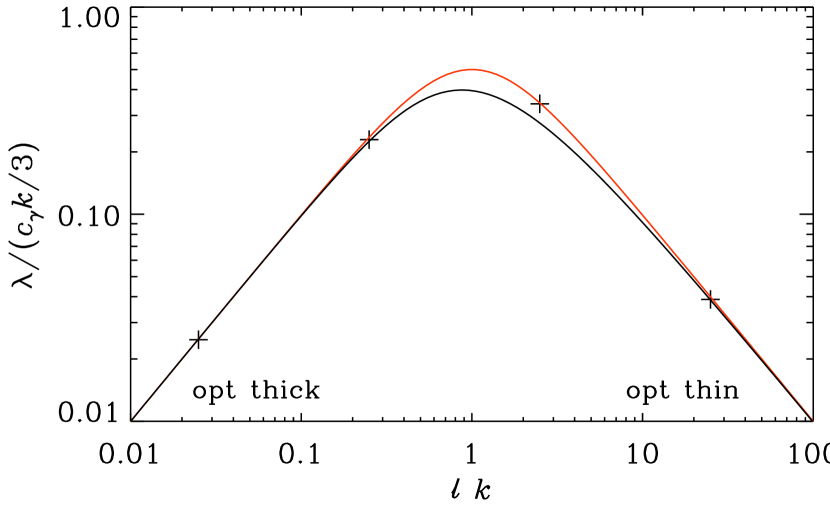
Figure 1: The analytic cooling curve (black), the cooling curve under the Eddington approximation (red), and the results from numerical simulations (plus signs).

Equations (4)–(6) apply to the case of three-dimensional (3-D) variations of the temperature. In our 3-D numerical experiments, however, we restrict ourselves to one-dimensional (1-D) variations of the mean temperature profile. In that case, the relevant version of Eq. (6) becomes BB14

$$\lambda\approx{c_{\gamma}\over\ell}\,{k^{2}\ell^{2}/3\over 1+k^{2}\ell^{2}}\quad\mbox{(1-D perturbations)}.$$ (7)

The corresponding version of Eq. (4) then takes the form

$$\lambda={c_{\gamma}\over\ell}\,\left(1-\frac{\arctan\sqrt{3}k\ell}{\sqrt{3}k\ell}\right)\quad\mbox{(1-D perturbations)}.$$ (8)

In Fig. 1, we compare $\lambda(k\ell)$ obtained from the exact equation (red curve) with the approximate $\lambda(k\ell)$ obtained under the Eddington approximation (black curve) for the relevant 1-D Equations (7) and (8). Our numerical solution for $\lambda$, which is based on only six rays, depends on the choice of weight factors used in the angular integration. The weight factors have been chosen such that our numerical results (plus signs) agree with the Eddington approximated solution BB14 . The basic question we want to answer is how the cooling curve gets modified in the presence of turbulence. We expect the effective $\lambda$ to be enhanced, at least in the optically thick limit, where $k\ell\ll 1$; however, we do not know what to expect in the optically thin case, where $k\ell\gg 1$, and how it depends on the scale of the turbulent eddies. To address these questions, we now perform turbulence simulations. We are particularly interested in the regime of moderate temperatures, where the radiation pressure can be ignored.

III Turbulence simulations

III.1 Comments on astrophysical conditions

The conditions in the Sun are extremely inhomogeneous owing to tremendous stratification. The density changes by nearly six orders of magnitude across the convection zone and the temperature by a factor of about 300. This fact alone can introduce new phenomena such as the spontaneous formation of magnetic flux concentrations BRK16 ; PB18 . At a more elementary level, the addition of gravity leads to convection and thereby to turbulent motions, which have been the subject of numerous simulations for a long time Nor82 ; SN98 . Newtonian cooling also plays important roles in the atmospheres of planets ZJBYAM21 , where turbulence is not always explicitly invoked and therefore the role of turbulence needs to be parameterized SPRS21 .

In the Sun, the microphysical viscosity is about twelve orders of magnitude smaller than the estimated turbulent viscosity, and over eight orders of magnitude smaller than the radiative diffusivity near the surface. Numerical simulations have therefore routinely employed numerical tools that allow the simulations to proceed by dissipating sufficient energy in local regions where necessary. This precluded the study of turbulent Newtonian cooling, because the small-scale turbulent motions have already been altered by such numerical modeling Leenaarts20 . An additional complication is partial ionization, which tends to make the transition from the deeper optically thick layers to the surface very sharp in a stratified system. However, one could imagine it to introduce new effects of its own if we arranged the average temperature of the domain such that it lies exactly in the middle between those of a fully ionized and a neutral medium, as has been done in some other recent experiments BB16 . In those cases, however, Newtonian cooling does not necessarily play any obvious role.

To accomplish our goal of identifying turbulent effects in optically thin and thick turbulent flows, we resort to the study of a minimal system where isotropic homogeneous turbulence is produced by a stirring force instead of convection. The viscosity is kept constant, but we consider different values to assess the dependence of our results on the Reynolds number. Partial ionization effects are ignored and other complications from adopting a realistic equation of state are not included. We also restrict our attention to the study of vortical forcing. The concept of turbulent mixing is likely to be similar also for irrotational forcing, but other poorly understood features of such turbulence such as a pileup of kinetic energy near the dissipative subrange (bottleneck effect) are known to occur in such cases MB06 . It may play a role in interstellar turbulence Fed10 , which motivates a more extended future study of turbulent Newtonian cooling for irrotational forcing.

III.2 Basic equations and thermodynamic relationships

For the purpose of our present study, we restrict ourselves to studying a turbulent flow in a triply periodic domain of size $L^{3}$ by applying plane wave forcing throughout the domain. We therefore solve the equations,

$$\rho{{\rm{D}}\bm{u}\over{\rm{D}}t}=-\mbox{\boldmath$\nabla$}{}p+\rho\bm{f}+\mbox{\boldmath$\nabla$}{}\bm{\cdot}(2\rho\nu\mbox{\boldmath${\sf S}$}{}),$$ (9)

$${{\rm{D}}\ln\rho\over{\rm{D}}t}=-\mbox{\boldmath$\nabla$}{}\bm{\cdot}\bm{u},$$ (10)

where $p$ is the pressure, $\bm{u}$ the velocity, and $\bm{f}$ the forcing function. In Eq. (9), we have ignored the radiation force $(\rho\kappa/c)\,\bm{F}_{\rm rad}$, where $c$ is the speed of light, as mentioned above. This term is unimportant for the temperatures considered in this work. Nevertheless, the coupled set of equations (1), (9), and (10) makes $s(\bm{x},t)$ an active scalar, because it is related to $p$ and $\rho$ through

$$s=c_{\rm v}\ln p-c_{\rm p}\ln\rho+s_{0},$$ (11)

where $c_{\rm v}$ is the specific heat at constant volume and $s_{0}$ is an irrelevant constant. This equation follows from the first law of thermodynamics, written in the form $T{\rm{d}}s={\rm{d}}e+p{\rm{d}}(\rho^{-1})$, where $e=c_{\rm v}T$ is the internal energy for a perfect gas, and the ideal gas equation relating the temperature to $p$ and $\rho$ through

$$(c_{\rm p}-c_{\rm v})\,T=p/\rho.$$ (12)

We then have ${\rm{d}}s=c_{\rm v}\,{\rm{d}}\ln T-(c_{\rm p}-c_{\rm v})\,{\rm{d}}\ln\rho$. Using the differentiated ideal gas equation, ${\rm{d}}\ln T+{\rm{d}}\ln\rho={\rm{d}}\ln p$, we arrive at Eq. (11) after integration. For the ratio of specific heats, $\gamma=c_{\rm p}/c_{\rm v}$, we assume $\gamma=5/3$, which is appropriate for a monatomic gas such as fully ionized hydrogen at the temperatures considered here ($T\approx 40,000\,{\rm K}$).

In our numerical work, we use dimensionful quantities, where length is measured in megameters (Mm), speed in $\,{\rm km\,s}^{-1}$, and temperature in kelvin. We also use the symbol $\nabla_{\rm ad}=1-1/\gamma=0.4$, which is the adiabatic value of what is in astrophysics commonly referred to as the double logarithmic temperature gradient, $\nabla\equiv{\rm{d}}\ln T/{\rm{d}}\ln p$ KW90 . Using this, $c_{\rm p}$ can then be written as $c_{\rm p}={\cal R}/(\mu\nabla_{\rm ad})$, where we have used $c_{\rm p}-c_{\rm v}={\cal R}/\mu$, with ${\cal R}=8.314\times 10^{7}\,{\rm cm}^{2}\,{\rm s}^{-2}\,{\rm K}^{-1}$ being the universal gas constant and $\mu=0.6$ the mean molecular weight. We then find $c_{\rm p}=0.035\,{\rm km}^{2}\,{\rm s}^{-2}\,{\rm K}^{-1}$.

III.3 Turbulent forcing

To simulate a turbulent flow, we apply nearly monochromatic forcing with an average forcing wavenumber $k_{\rm f}$. The forcing function changes abruptly from one time step to the next, i.e., $\langle\bm{f}(\bm{x},t)\bm{f}(\bm{x},t^{\prime})\rangle$ is proportional to $\delta(t-t^{\prime})$, where $\delta$ is the Dirac $\delta$ function. The forcing is then said to be $\delta$ correlated in time. The smallest wavenumber in the cubic domain of side length $L$ is $k_{1}=2\pi/L$. The ratio $k_{\rm f}/k_{1}$ is the scale separation ratio, for which we consider the values 1.5 and 10.

For the forcing function $\bm{f}$, we select randomly at each time step a phase $-\pi<\varphi\leq\pi$ and the components of the wavevector $\bm{k}$ from many possible discrete wavevectors with lengths in a certain range around a given value $k_{\rm f}$. In this way, the adopted forcing function

$$\bm{f}(\bm{x},t)={\rm Re}\{{\cal N}\tilde{\bm{f}}(\bm{k},t)\exp[i\bm{k}\cdot\bm{x}+i\varphi]\}$$ (13)

is white noise in time and consists of plane waves with average wavenumber $k_{\rm f}$. Here, $\bm{x}$ is the position vector and ${\cal N}=f_{0}(c_{\rm s0}k_{\rm f}\delta t)^{1/2}$ is a normalization factor, where $\delta t$ is the time step and $f_{0}$ is an amplitude factor. In this formulation, the averaged forcing is independent of $\delta t$. To ensure that $\tilde{\bm{f}}$ is solenoidal, i.e., perpendicular to $\bm{k}$, we write is as

$$\tilde{\bm{f}}({\bm{k}})=(\bm{k}\times\bm{\hat{e}})/[\bm{k}^{2}-(\bm{k}\cdot\bm{\hat{e}})^{2}]^{1/2},$$ (14)

where $\bm{\hat{e}}$ is an arbitrary unit vector that are not aligned with $\bm{k}$. Note that $|\bm{f}|^{2}=1\,{\rm km}^{4}\,{\rm s}^{-4}\,{\rm Mm}^{-2}$. The coefficient $f_{0}$ is chosen such that the velocity is about 10% of the sound speed.

III.4 Initial temperature profile and parameters

We adopt a sinusoidal temperature perturbation and write $T(x,t=0)$ in the form

$$T(x,t=0)\,=\,T_{0}+T_{1}\sin kx,$$ (15)

where $k=k_{1}=1\,{\rm Mm}^{-1}$ is chosen. This implies that $L=2\pi\,{\rm Mm}\approx 6.28\,{\rm Mm}$. We choose $c_{\rm s0}=30\,{\rm km\,s}^{-1}$, so that $T_{0}\approx 40,000\,{\rm K}$ and $c_{\gamma}=3.9\,{\rm km\,s}^{-1}$. The temperature perturbation is taken to be $T_{1}=2000\,{\rm K}$, and periodic boundary conditions are assumed for all quantities.

We define the Mach and Reynolds numbers as

$${\rm{Ma}}=u_{\rm rms}/c_{\rm s0},\quad{\rm{Re}}=u_{\rm rms}/\nu k_{\rm f}.$$ (16)

For a forcing amplitude $f_{0}=0.01\,{\rm km}^{2}\,{\rm s}^{-2}\,{\rm Mm}^{-1}$, we have $u_{\rm rms}\approx 2.2\,{\rm km\,s}^{-1}$, so that ${\rm{Ma}}\approx 0.08$. Using $\nu=10^{-3}\,{\rm Mm}\,{\rm km}\,{\rm s}^{-1}$ and $k_{\rm f}=10\,{\rm Mm}^{-1}$, we have ${\rm{Re}}\approx 230$, while for $k_{\rm f}=1.5\,{\rm Mm}^{-1}$, we have ${\rm{Re}}\approx 1200$. To determine the microphysical Prandtl number in the optically thick regime, we define

$${\rm{Pr}_{0}}=3\nu k_{1}/c_{\gamma},$$ (17)

so that the Prandtl number is $\nu/\chi={\rm{Pr}_{0}}/(k_{1}\ell)$. Here we have used $\chi=c_{\gamma}\ell/3$ for the radiative diffusivity. Following earlier work BB14 , we choose for the mean density the value $\rho_{0}=4\times 10^{-4}\,{\rm g}\,{\rm cm}^{-3}$.

We determine the effective $\lambda$ from the time evolution of the decay of the sinusoidal perturbation, which we monitor by taking the difference between the maximum and minimum temperatures at each time. This turns out to be reasonably accurate and we use a time interval during which the decay is exponential.

III.5 Numerical technique

We perform numerical simulations with the Pencil Code (https://github.com/pencil-code), which is a public MHD code that is particularly well suited for simulating turbulence PencilCollab . We solve Eqs. (1), (9), and (10) with sixth-order finite differences Bra03 . Equation (3) is solved with second-order accurate finite differences along the coordinate directions and the diagonals, i.e., altogether 26 rays. The radiation transport has been parallelized in the Pencil Code by splitting the calculation into parts that are local and nonlocal with respect to each processor HDNB06 . Two parts are compute-intensive, but require no communication, and one part is nonlocal, but does not require waiting for any computation to be done and is therefore fast. We use the third-order time-stepping scheme of Williamson Wil80 .

The code’s local cooling and heating properties have been verified BB14 , and its cooling time has been compared with the analytic cooling time obtained by Spiegel Spi57 . It is this cooling time that determines the relevant time step constraint for radiation simulations Freytag12 ; BD20 , and not some generalization of the usual Courant condition DSJ12 . The latter would erroneously imply a limiting time step that is proportional to the mesh spacing, when it is actually quadratic in the mesh spacing in the optically thick limit and independent of mesh spacing in the optically thin limit.

The code has been applied to sunspot simulations HNSS07 , and to a range of more idealized problems of atmospheric stability BB14 and magnetic spot formation BB16 ; PB18 . It should be emphasized that our calculations classify as direct numerical simulations in the sense that the equations are solved as stated, albeit with unrealistically large viscosity and unrealistically small opacities compared with solar conditions. By comparison, most simulations of solar convection are performed using large eddy simulations SN98 ; Rem09 ; Freytag12 .

III.6 Comment on numerical convergence and accuracy

The fact that the Pencil Code uses sixth-order finite differences and a third-order time-stepping scheme does not tell us much about the actual accuracy and convergence of our results. For example, the longer a simulation, the more numerical errors should accumulate, but this is not normally seen. This was recently addressed in a study comparing the numerical accuracy of turbulence and waves RPBKKM20 . In that study, it was concluded that the existence of a forward cascade in turbulence prevents the systematic loss of energy at small scales, where discretization errors are the largest. This is not the case for waves, which therefore need to be solved with much more care. Another such example was a recent three-dimensional study of electromagnetic waves BS21 . In this and the previous case, it proved advantageous to use an exact time integration under the assumption that the turbulent source is unchanged between two time steps. This approximation is justified because at high wavenumbers, the relevant timescale of waves is much shorter than that of turbulence RPBKKM20 .

Also radiation can introduce short time scales. As already alluded to in the beginning, the cooling time can be very short and severely restrict the relevant time step constraint Freytag12 ; BD20 . This makes the simulations very costly DSJ12 , but we are not aware of any reports on loss of accuracy in such cases. Furthermore, in the present studies, we are probably not affected by this constraint, because turbulent Newtonian cooling only plays a role when the turbulent time scales are short compared with radiative ones. This is here not the case.

Table 1: Summary of the parameters for the series of runs presented in this paper. Within each series of runs, $\kappa$ and $\ell$ are varied.

Series $k/k_{1}$ $k_{\rm f}/k_{1}$ $u_{\rm rms}/c_{\gamma}$ ${\rm{Pr}_{0}}$ ${\rm{Re}}$ $N^{3}$ A’ 1 10 0.50 $8\times 10^{-3}$ 20 $64^{3}$ A 1 10 0.59 $8\times 10^{-4}$ 230 $256^{3}$ B 1 1.5 0.62 $8\times 10^{-3}$ 160 $64^{3}$ C 3 1.5 0.46 $8\times 10^{-4}$ 1200 $256^{3}$ D 6 1.5 0.46 $8\times 10^{-4}$ 1200 $256^{3}$

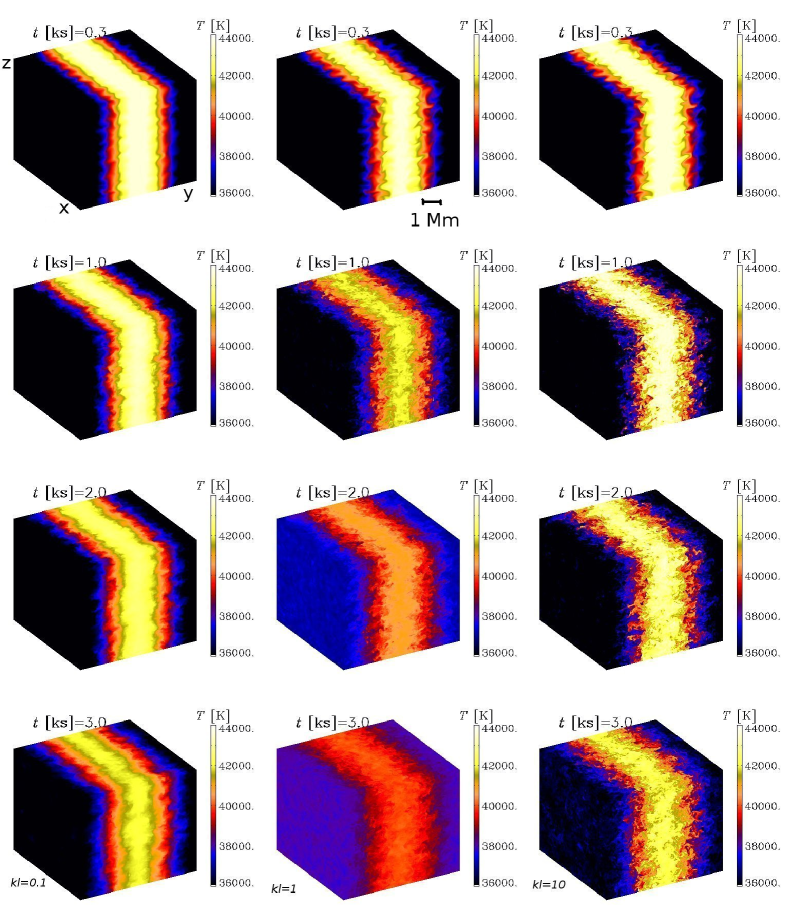
Figure 2: Temperature on the periphery of the computational domain for $k\ell=0.1$ (left column), $k\ell=1$ (middle column), and $k\ell=10$ (right column), for $t=0.3\,{\rm ks}$, $t=1\,{\rm ks}$, $t=2\,{\rm ks}$, and $t=3\,{\rm ks}$ (top to bottom). The $(x,y,z)$ coordinates are indicated in the first panel and the approximate $1\,{\rm Mm}$ scale is shown in the second panel.

IV Results

IV.1 Range of simulations and qualitative aspects

In this section, we present the results for $\lambda$ obtained using various values of the forcing wavenumber $k_{\rm f}$ and the wavenumber $k$ of the initial perturbation. The Reynolds number varies between 20 and 1200, and the number of mesh points, $N^{3}$, is varied between $64^{3}$ and $256^{3}$; see Table LABEL:Tsum. The values of ${\rm{Pr}_{0}}$ are then small, as is also expected for the Sun, and they are $8\times 10^{-3}$ for our runs with $64^{3}$ mesh points (small Reynolds numbers) and $8\times 10^{-4}$ for $256^{3}$ mesh points (larger Reynolds numbers). For each series of runs, we perform simulations where we vary the opacity $\kappa$ and thereby $\ell$; see Fig. 2 for visualizations of $T$ on the periphery of the computational domain for runs of Series A for $k\ell=0.1$, $1$, and $10$ and at different times (in kiloseconds [ks]). We see that the large-scale temperature contrast (wavenumber $k=k_{1}$) decreases the fastest for $k\ell=1$, and more slowly for $k\ell=0.1$ and $10$. For $k\ell=10$, however, which is the optically thin case, the temperature retains smaller scale structures for longer.

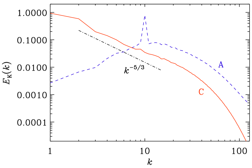
Figure 3: Kinetic energy spectra for Series A (dashed blue) and Series C (solid red). The $k^{-5/3}$ slope is overplotted for comparison.

IV.2 Kinetic energy spectra

In spite of the forcing being monochromatic, the resulting turbulence is excited over a broad range of scales. This is demonstrated in Fig. 3, where we plot kinetic energy spectra, $E_{\rm K}(k)=\int|\tilde{\bm{u}}|^{2}k^{2}{\rm{d}}\Omega_{k}$, for Series A and C. Here, $\tilde{\bm{u}}$ is the Fourier transformation of $\bm{u}$, and ${\rm{d}}\Omega_{k}$ is the solid angle differential in wavenumber space. The spectra are normalized such that $\int E_{\rm K}(k)\,{\rm{d}}k=u_{\rm rms}^{2}/2$. In the case of Series C, where ${\rm{Re}}=1200$ and $k_{\rm f}/k_{1}=1.5$, there is a short inertial range $\propto k^{-5/3}$ together with a bottleneck, i.e., a shallower spectrum near the dissipative subrange Fal94 ; Zheng21 . We note that the bottleneck effect is physical, but much weaker in the one-dimensional spectra that are accessible to laboratory and atmospheric measurements Dobler . It is also seen in the highest resolution turbulence simulations today Fed21 .

In the simulations with larger scale separation (Series A), however, the spectrum is more peaked around $k=k_{\rm f}$. This occurrence of this spike at $k_{\rm f}$ is partially explained by the smaller Reynolds number (${\rm{Re}}=230$ in this case).

In general, higher scale separation allows us to see more clearly the various mean-field effects. In this connection, we must remember that the standard concept of turbulent diffusion does require sufficient scale separation and that the lack of scale separation requires one to study the full scale dependence, in which case turbulent diffusion corresponds to an integral kernel in real space, or a multiplication with a $k$-dependent diffusivity in Fourier space BRS08 . For this reason, we also discuss the aspect of scale dependence below.

IV.3 Quantitative results for turbulent cooling

In Fig. 4, we plot $\lambda$ versus $k\ell$ and compare with the laminar case shown in Fig. 1. In all the cases, we see that $\lambda$ is enhanced relative to the laminar curve. Varying the viscosity, and thereby changing ${\rm{Re}}$ from 20 (Series A’) to 230 (Series A), has a very minor effect; compare the dotted and solid blue lines for $k/k_{\rm f}=0.1$ in Fig. 4. Decreasing $k_{\rm f}/k_{1}$ from 10 to 1.5, that is, increasing $k/k_{\rm f}$ from 0.1 (Series A) to 0.7 (Series B), has a more significant effect, and $\lambda$ is seen to increase by a factor that is between 4 and 8, depending on the value of $k\ell$.

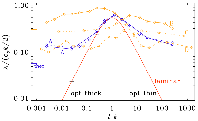
Figure 4: Effective turbulent decay rate $\lambda$ versus $k\ell$ for Series A’ (dotted blue), A (solid blue), B (solid orange), C (dotted orange), and D (dashed orange). The short lines on the left $y$ axis, with line types matching those of the curves in the plot, give the theoretical expectations explained in the text. The curve for the laminar case is shown in red.

Keeping the value of $k_{\rm f}$ unchanged and increasing $k/k_{\rm f}$ (for Series C and D), i.e., making the scale separation poorer, results in a weak decline of $\lambda$. Theoretically, we would expect the turbulent decay rate to be $\lambda=\chi_{\rm t}k^{2}$, where $\chi_{\rm t}=\chi_{\rm t0}\equiv u_{\rm rms}/3k_{\rm f}$ is the nominal turbulent diffusivity in the case of perfect scale separation. For poor scale separation, however, we expect $\chi_{\rm t}=\chi_{\rm t0}/[1+(k/k_{\rm f})^{2}]$. We see from the short lines overplotted on the left $y$ axis of Fig. 4 that the actual decay rates are somewhat larger.

We note that in Fig. 4, the decay rates of lines having different values of $k$ (but the same value of $k_{\rm f}$) are all separated by factors that are close to $k$ itself. To demonstrate that this is mostly the result of normalizing $\lambda/c_{\gamma}$ by $k$, we show in Fig. 5 the result of normalizing $\lambda/c_{\gamma}$ by $k_{1}$, which is the same for all runs. The lines are now no longer so strongly separated for different values of $k$. Note that the abscissa is also scaled by $k_{1}$ instead of $k$. Consequently, the small peaks in $\lambda$ values near $k_{1}\ell=1$ occur at similar positions.

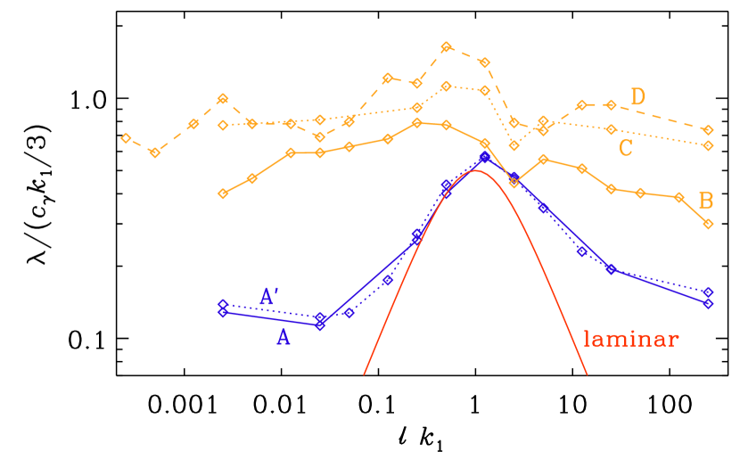
Figure 5: Similar to Fig. 4, but the abscissa is scaled with $k_{1}$ instead of $k$, and the ordinate is divided by $k_{1}$ instead of $k$. Again, Series A’ and A are denoted by dotted and solid blue lines, respectively, and Series B, C, and D, are denoted by solid, dotted, and dashed orange lines, respectively. The curve for the laminar case is shown again in red.

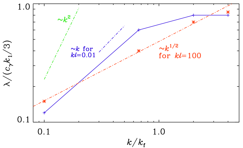
Figure 6: Dependence of $\lambda/(c_{\gamma}k_{1}/3)$ on $k/k_{\rm f}$ for $k\ell=0.01$ (blue, optically thick), and $k\ell=100$ (red, optically thin). The later obeys a $k^{1/2}$ scaling. For comparison, we also show the linear scaling in $k$ (blue) and the quadratic scaling (green).

IV.4 Scale dependence

The standard concept of turbulent diffusion with a diffusion operator of the form $\chi_{\rm t}\nabla^{2}$ requires one to have sufficient scale separation, as is the case for our runs of Series A. If scale separation is poor, the operator $\chi_{\rm t}\nabla^{2}$ has to be replaced by a convolution in real space BRS08 . This subject continues to attract significant attention, especially in plasma physics BC20 and astrophysics GE20 ; BenS21 .

In Fig. 6 we summarize the results for $\lambda/(c_{\gamma}k_{1}/3)$ as a function of $k/k_{\rm f}$ for $k\ell=0.01$ (optically thick regime), and $k\ell=100$ (optically thin regime). Neither of the two regimes exhibits a $k^{2}$ dependence, as would be expected for a turbulent diffusion process with $k/k_{\rm f}\ll 1$, i.e., when the turbulent diffusivity is approximately scale-independent. In the optically thick case, $\lambda$ increases approximately linearly with $k$ for small values of $k$ and then reaches a maximum. In the optically thin case, on the other hand, $\lambda$ increases with $k$ approximately like $k^{1/2}$.

Figure 7: Dependence of the passive scalar diffusion rate $\kappa_{\rm t}(k)k^{2}$ on $k/k_{\rm f}$ for scale separations $k_{\rm f}/k_{1}=3$ and 8.

IV.5 Analogy with passive scalar diffusion

In the optically thick regime, $k\ell\ll 1$, where the radiative diffusion approximation should be applicable, we might expect some analogy between turbulent diffusion of active scalars (such as temperature) and passive scalars (such as chemical concentrations). For the latter, the scale dependence has previously been investigated BSV09 , and it was found to be similar to that for magnetic fields BRS08 in that both had a Lorentzian shape. In these papers, the microphysical and turbulent diffusivities were referred to as $\kappa$ and $\kappa_{\rm t}$ for the passive scalar BSV09 (not to be confused with the opacity in the present paper) and $\eta$ and $\eta_{\rm t}$ for the magnetic diffusivity BRS08 . They have the same meaning as $\chi$ and $\chi_{\rm t}$ in the present paper. In these cases, we plot the time scale on which a large-scale sinusoidal profile of the passive scalar or the magnetic field gets diffused away.

We reproduce in Fig. 7 the result from the test-field method for passive scalars BSV09 . These authors also studied the effects of rotation and magnetic fields, but those results were not used for the present comparison. Their passive scalar diffusivity $\kappa_{\rm t}$ obeyed a Lorentzian fit such that

$$\kappa_{\rm t}(k)={u_{\rm rms}/3k_{\rm f}\over 1+(ak/k_{\rm f})^{2}},$$ (18)

where $a=0.62$ is an empirical parameter. The corresponding decay rate, $\kappa_{\rm t}k^{2}$, is normalized by $u_{\rm rms}k_{1}/3$ and shows a clear quadratic growth for small $k$ and levels off near $k=k_{\rm f}$, as expected.

Similar Lorentzian fits have been found over a broad range of different applications to turbulent magnetic diffusion: values of $a\approx 0.5$, $a\approx 0.7$, and $a\approx 0.2$ were found for isotropic turbulence BRS08 , anisotropic turbulence with shear MKTB09 , and passive scalar diffusivity with shear MB10 , respectively.

V Conclusions

Our work has demonstrated that the concept of turbulent diffusion carries over to radiative turbulent diffusion as well, in both optically thick and thin limits. While this was expected for the optical thick limit, it was not obvious how this would be modified in the optically thin limit, which is not a diffusion process. Instead, the optically thin case is characterized by Newtonian cooling, which then turns into turbulent Newtonian cooling. Both processes are shown to be scale-dependent, i.e., they are really described by integral kernels.

We can now also answer the question regarding the combined effect of decreased turbulence and small optical depth on the cooling at small length scales. As we have seen, turbulence always enhances the microphysical cooling rates. Thus, at small length scales where radiative diffusion is replaced by the much less efficient Newtonian cooling, turbulence speeds up this effect again. Mathematically, this process is still treated like Newtonian cooling, but now with a cooling time that is no longer given by $\ell/c_{\gamma}$, but by the turbulent turnover time $(u_{\rm rms}k_{\rm f})^{-1}$. Radiation no longer enters explicitly, except through the condition $k\ell>1$ for turbulent Newtonian cooling, as opposed to $k\ell<1$ for turbulent radiative diffusion.

As for the scope of future work, independent verifications of our results would certainly be desirable. In particular, it is conceivable that one can develop a test-field method similar to that employed for passive scalars BSV09 . It would also be useful to study the effects of turbulent radiative diffusion and turbulent Newtonian cooling by comparing direct numerical simulations with mean-field models. This could be particularly insightful in more realistic situations involving stratification, turbulence, and magnetic fields, which could give rise to interesting phenomena such as magnetic spot formation BRK16 ; PB18 .

Conflict of interest

The authors have no conflicts to disclose.

Data Availability Statement

The source code used for the simulations in this study, the Pencil Code PC , is freely available on https://github.com/pencil-code/. The DOI of the code is https://doi.org/10.5281/zenodo.2315093. The simulation setup and the corresponding data Brandenburg (2020) are freely available on https://doi.org/10.5281/zenodo.4085411.

References

- (1) G. Rüdiger, Reynolds stresses and differential rotation I. On recent calculations of zonal fluxes in slowly rotating stars, Geophys. Astrophys. Fluid Dynam. 16, 239–261 (1980).
- (2) H. K. Moffatt Magnetic Field Generation in Electrically Conducting Fluids. Cambridge: Cambridge Univ. Press (1978).
- (3) F. Krause and K.-H. Rädler Mean-field Magnetohydrodynamics and Dynamo Theory. Oxford: Pergamon Press (1980).
- Rädler et al. (2011) K.-H. Rädler, A. Brandenburg, F. Del Sordo, and M. Rheinhardt, Mean-field diffusivities in passive scalar and magnetic transport in irrotational flows, Phys. Rev. E 84, 4 (2011).
- (5) E. Schatzman Cosmic gas dynamics: Part 1. Cosmic gas dynamics; see p. 50. New York: Wiley-Interscience (1974).
- (6) A. Brandenburg and U. Das, The time step constraint in radiation hydrodynamics, Geophys. Astrophys. Fluid Dynam. 114, 162–195 (2020).
- (7) A. Brandenburg, K.-H. Rädler, and M. Schrinner, Scale dependence of alpha effect and turbulent diffusivity, Astron. Astrophys. 482, 739–746 (2008).
- (8) A. Brandenburg, A. Svedin, and G. M. Vasil, Turbulent diffusion with rotation or magnetic fields, Month. Not. Roy. Astron. Soc. 395, 1599–1606 (2009).
- (9) K.-H. Rädler, “Mean-Field Magnetohydrodynamics as a Basis of Solar Dynamo Theory,” In Basic Mechanisms of Solar Activity, Proceedings from IAU Symposium No. 71 held in Prague, Czechoslovakia (ed. V. Bumba and J. Kleczek), pp. 323–344. D. Reidel Publishing Company Dordrecht (1976).
- (10) W. Unno and E. A. Spiegel, The Eddington approximation in the radiative heat equation, Publ. Astron. Soc. Jap. 18, 85-95 (1966).
- (11) Å. Nordlund, Numerical simulations of the solar granulation I. Basic equations and methods, Astron. Astrophys. 107, 1–10 (1982).
- (12) E.-J. Rijkhorst, T. Plewa, A. Dubey, and G. Mellema, Hybrid characteristics: 3D radiative transfer for parallel adaptive mesh refinement hydrodynamics, Astron. Astrophys. 452, 907–920 (2006).
- (13) E. A. Spiegel, The smoothing of temperature fluctuations by radiative transfer, Astrophys. J. 126, 202–207 (1957).
- (14) A. Barekat and A. Brandenburg, Near-polytropic stellar simulations with a radiative surface, Astron. Astrophys. 571, A68 (2014).
- Edwards (1990) J. M. Edwards, Two-dimensional radiative convection in the Eddington approximation, Month. Not. Roy. Astron. Soc. 242, 224–234 (1990).
- (16) A. Brandenburg, I. Rogachevskii, and N. Kleeorin, Magnetic concentrations in stratified turbulence: the negative effective magnetic pressure instability, New J. Phys. 18, 125011 (2016).
- (17) B. Perri and A. Brandenburg, Spontaneous flux concentrations from the negative effective magnetic pressure instability beneath a radiative stellar surface, Astron. Astrophys. 609, A99 (2018).
- (18) R. F. Stein and Å. Nordlund, Simulations of solar granulation: I. General properties, Astrophys. J. 499, 914–933 (1998).
- (19) Z. Zhu, Y.-F. Jiang, H. Baehr, A. N. Youdin, P. J. Armitage, and R. G. Martin, Global 3D radiation hydrodynamic simulations of proto-Jupiter’s convective envelope, Month. Not. Roy. Astron. Soc., submitted, arXiv:2106.12003 (2021).
- (20) L. Soucasse, B. Podvin, P. Rivière, and A. Soufiani, Low-order models for predicting radiative transfer effects on Rayleigh-Bénard convection in a cubic cell at different Rayleigh numbers, J. Fluid Mech. 917, A5 (2021).
- (21) J. Leenaarts, Radiation hydrodynamics in simulations of the solar atmosphere, Liv. Rev. Sol. Phys. 17, 3 (2020).
- (22) P. Bhat and A. Brandenburg, Hydraulic effects in a radiative atmosphere with ionization, Astron. Astrophys. 587, A90 (2016).
- (23) A. J. Mee and A. Brandenburg, Turbulence from localized random expansion waves, Month. Not. Roy. Astron. Soc. 370, 415–419 (2006).
- (24) C. Federrath, J. Roman-Duval, R. S. Klessen, W. Schmidt, and M.-M. Mac Low, Comparing the statistics of interstellar turbulence in simulations and observations. Solenoidal versus compressive turbulence forcing, Astron. Astrophys. 512, A81 (2010).
- (25) R. Kippenhahn and A. Weigert Stellar structure and evolution. Springer: Berlin (1990).
- (26) Pencil Code Collaboration: A. Brandenburg, A. Johansen, P. A. Bourdin, W. Dobler, W. Lyra, M. Rheinhardt, S. Bingert, N. E. L. Haugen, A. Mee, F. Gent, N. Babkovskaia, C.-C. Yang, T. Heinemann, B. Dintrans, D. Mitra, S. Candelaresi, J. Warnecke, P. J. Käpylä, A. Schreiber, P. Chatterjee, M. J. Käpylä, X.-Y. Li, J. Krüger, J. R. Aarnes, G. R. Sarson, J. S. Oishi, J. Schober, R. Plasson, C. Sandin, E. Karchniwy, L. F. S. Rodrigues, A. Hubbard, G. Guerrero, A. Snodin, I. R. Losada, J. Pekkilä, and C. Qian, The Pencil Code, a modular MPI code for partial differential equations and particles: multipurpose and multiuser-maintained, J. Open Source Software 6, 2807 (2021).
- (27) A. Brandenburg, “Computational aspects of astrophysical MHD and turbulence,” In Advances in nonlinear dynamos (The Fluid Mechanics of Astrophysics and Geophysics, Vol. 9) (ed. A. Ferriz-Mas & M. Núñez), pp. 269–344. Taylor & Francis, London and New York (2003).
- (28) T. Heinemann, W. Dobler, Å. Nordlund, and A. Brandenburg, Radiative transfer in decomposed domains, Astron. Astrophys. 448, 731–737 (2006).
- (29) J. H. Williamson, Low-storage Runge-Kutta schemes, J. Comp. Phys. 35, 48–56 (1980).
- (30) B. Freytag, M. Steffen, H.-G. Ludwig, S. Wedemeyer-Böhm, W. Schaffenberger, and O. Steiner, Simulations of stellar convection with CO5BOLD, J. Comp. Phys. 231, 919–959 (2012).
- (31) S. W. Davis, J. M. Stone, and Y. F. Jiang, A radiation transfer solver for Athena using short characteristics, Astrophys. J. 199, 9 (2012).
- (32) T. Heinemann, Å. Nordlund, G. B. Scharmer, and H. C. Spruit, MHD simulations of penumbra fine structure, Astrophys. J. 669, 1390–1394 (2007).
- (33) M. Rempel, M. Schüssler, and M. Knölker, Radiative magnetohydrodynamic simulation of sunspot structure, Astrophys. J. 691, 640–649 (2009).
- (34) A. Roper Pol, A. Brandenburg, T. Kahniashvili, A. Kosowsky, and S. Mandal, The timestep constraint in solving the gravitational wave equations sourced by hydromagnetic turbulence, Geophys. Astrophys. Fluid Dynam. 114, 130–161 (2020).
- (35) A. Brandenburg and R. Sharma, Simulating relic gravitational waves from inflationary magnetogenesis, Astrophys. J., in press, arXiv:2106.03857 (2021).
- (36) G. Falkovich, Bottleneck phenomenon in developed turbulence, Phys. Fluids 6, 1411–1414 (1994).
- (37) Q. Zheng, J. Wang, M. M. Alam, B. R. Noack, H. Li, and S. Chen, Transfer of internal energy fluctuation in compressible isotropic turbulence with vibrational non-equilibrium, J. Fluid Mech. 919, 26 (2021).
- (38) W. Dobler, N. E. L. Haugen, T. A. Yousef, and A. Brandenburg, Bottleneck effect in three-dimensional turbulence simulations, Phys. Rev. E 68, 026304 (2003).
- (39) C. Federrath, R. S. Klessen, L. Iapichino, and J. R. Beattie, The sonic scale of interstellar turbulence, Nat. Astron. 5, 365–371 (2021).
- (40) A. Brandenburg and L. Chen, The nature of mean-field generation in three classes of optimal dynamos, J. Plasma Phys. 86, 905860110 (2020).
- (41) O. Gressel and D. Elstner, On the spatial and temporal non-locality of dynamo mean-field effects in supersonic interstellar turbulence, Month. Not. Roy. Astron. Soc. 494, 1180–1188 (2020).
- (42) A. B. Bendre and K. Subramanian, Non-locality of the turbulent electromotive force, Phys. Rev. Lett., submitted, arXiv:2107.10625 (2021).
- (43) D. Mitra, P. J. Käpylä, R. Tavakol, and A. Brandenburg, Alpha effect and diffusivity in helical turbulence with shear, Astron. Astrophys. 495, 1–8 (2009).
- (44) E. J. M. Madarassy and A. Brandenburg, Calibrating passive scalar transport in shear-flow turbulence, Phys. Rev. E 82, 016304 (2010).
- (45) A. Brandenburg and W. Dobler, Pencil Code, Astrophysics Source Code Library, ascl:1010.060, http://ui.adsabs.harvard.edu/abs/2010ascl.soft10060B, DOI:10.5281/zenodo.2315093.
- Brandenburg (2020) A. Brandenburg and U. Das, 2020, Datasets for “Turbulent radiative diffusion and turbulent Newtonian cooling,” v2020.10.13, Zenodo, DOI:10.5281/zenodo.4085411