Fast signal recovery from quadratic measurements

Abstract

We present a novel approach for recovering a sparse signal from cross correlated data. The bottleneck for inversion in this case is the number of unknowns that grows quadratically, resulting in a prohibitive computational cost as the dimension of the problem increases. The main feature of the proposed approach is that its cost is similar to the one of the usual sparse signal recovery problem with linear measurements. The keystone of the methodology is the use of a Noise Collector that absorbs the data component that comes from the off-diagonal elements of the unknown matrix formed by the cross correlation of the original unknown vector. The data component that is absorbed this way does not carry extra information about the support of the signal and, thus, we can safely reduce the dimensionality of the problem making it competitive with respect to the one that uses linear data. Our theory shows that the proposed approach provides exact support recovery when the data is not too noisy and that there are no false positives for any level of noise. Moreover, our theory also demonstrates that when using cross correlated data, the level of sparsity that can be recovered increases, scaling almost linearly with the number of data. The numerical experiments presented in the paper corroborate these findings.

Keywords: quadratic data, $\ell_{1}$-minimization, noise, model reduction

1 Introduction

Reconstruction of signals from cross correlations has interesting applications in many fields of science and engineering such as optics, quantum mechanics, electron microscopy, antenna testing, seismic interferometry, or imaging in general [9, 12, 21, 19]. Using cross correlations of measurements collected at different locations presents several advantages since the inversion does not require knowledge of the emitter positions, or the probing pulses shapes as only time differences matter. Cross correlations have been used, for example, when imaging is carried out with opportunistic sources whose properties are mainly unknown [7, 8, 6, 13].

In many applications, we seek information about an object or a signal $\mbox{\boldmath$\rho$}\in\mathcal{C}^{K}$ given data $\mbox{\boldmath$b$}\in\mathcal{C}^{N}$ most often related through a linear transformation

$${\cal A}\,\mbox{\boldmath$\rho$}=\mbox{\boldmath$b$}\,,$$ (1)

where ${\cal A}\in\mathcal{C}^{N\times K}$ is the measurement or model matrix. When the signal $\rho$ is compressed or when the data is scarce, $N<K$, in which case (1) is underdetermined and infinitely many signals or objects match the data. However, if the signal $\rho$ is sparse so only $M\ll K$ components are different than zero, $\ell_{1}$-minimization algorithms that solve

$$\mbox{\boldmath$\rho$}_{\ell_{1}}=\mathop{\mbox{argmin}}\|\mbox{\boldmath{$\rho$}}\|_{\ell_{1}},\hbox{ subject to }{\cal A}\mbox{\boldmath{$\rho$}}=\mbox{\boldmath{$b$}}\,$$ (2)

can recover the true signal efficiently even when $N\ll K$.

On the other hand, there are situations in which it is difficult or impossible to record high quality data, $b$, and it is more convenient to use the cross correlated data contained in the matrix

$$B=\mbox{\boldmath$b$}\,\mbox{\boldmath$b$}^{*}\in\mathcal{C}^{N\times N}\,$$ (3)

to find the desired information about the object or signal $\rho$ (see [7] and references therein). One way to address this problem is to lift it to the matrix level and reformulate it as a low-rank matrix linear system, which can be solved by using nuclear norm minimization as it was suggested in [4, 3] for imaging with intensities-only. This makes the problem convex over the appropriate matrix vector space and, thus, the unique true solution can be found using well established algorithms involving are not as efficient as $\ell_{1}$-minimization algorithms that only involve lightweight operations such as matrix-vector multiplications [1]. Furthermore, the big caveat is that the computational cost rapidly becomes prohibitively large as the dimension of the problem increases quadratically with $K$, making its solution infeasible.

In this paper we suggest a different approach. We propose to consider the linear matrix equation

$${\cal A}X{\cal A}^{*}=B\,$$ (4)

for the correlated signal $X=\mbox{\boldmath$\rho$}\,\mbox{\boldmath$\rho$}^{*}\in\mathcal{C}^{K\times K}$, vectorize both sides so

$$\mbox{vec}({\cal A}X{\cal A}^{*})=\mbox{vec}(B)\,,$$ (5)

and use the Kronecker product $\otimes$, and its property $\mbox{vec}(PQR)=(R^{T}\otimes P)\mbox{vec}(Q)$, to express the matrix multiplications as the linear transformation

$$({\bar{\cal A}}\otimes{\cal A})\,\mbox{vec}(X)=\mbox{vec}(B)\,.$$ (6)

Thus, we can promote the sparsity of the sought image using $\ell_{1}$-minimization algorithms that are much faster than nuclear norm minimization ones. However, the dimension of the unknown $\mbox{vec}(X)$ in (6) also increases quadratically with $K$, so this approach by itself would still be impractical when $K$ is not very small.

Hence, we propose to use a Noise Collector to reduce the dimensionality of problem (6). The Noise Collector was introduced in [17] to eliminate the clutter in the recovered signals when the data are contaminated by additive noise. In this paper, we use the Noise Collector to absorb part of the signal instead. Specifically, we treat as noise the signal that corresponds to the $K^{2}-K$ off-diagonal entries in the matrix $X$. Using the Noise Collector allows us to ignore these entries and construct a linear system with the same number of unknowns as the original problem (1) that uses linear data. As a consequence a dimension reduction from $K^{2}$ to $K$ unknowns is achieved. The main result of this paper is Theorem 3 which says that under certain decoherence conditions on the matrix ${\cal A}$, we can find the support of an M-sparse signal exactly if the data is noise-free or the noise is low enough. Furthermore, Theorem 3 shows that the level of sparsity $M$ that can be recovered increases from $O(\sqrt{N}/\sqrt{\ln N})$ to $O(N/\sqrt{\ln N})$ when quadratic cross correlation data are used instead of the linear ones.

The numerical experiments included in this paper support the results of Theorem 3. They show that the support of a signal can be found exactly if the noise in the data is not too large with almost no extra computational cost with respect to the original problem (1) that considers linear data with no correlations. Once the support has been found, a trivial second step allows us to find the signal, including its phases. The reconstruction is exact when there is no noise in the data and the results are very satisfactory even for noisy data with low signal to noise ratios. That is, our numerical experiments suggest that the approach presented here is robust with respect to additive noise. Additional properties of this approach are that for any level of noise the solution has no false positives, and that the algorithm is parameter-free, so it does not require an estimation of the energy of the off-diagonal signal that we need to absorb, or of the level of noise in the data.

The paper is organized as follows. In Section 2, we summarize the model used to generate the signals to be recovered, which in our case are images. In Section 3, we present the theory that supports the proposed strategy for dimension reduction when correlated data are used to recover the signals. Section 4 explains the algorithm for carrying out the inversion efficiently. Section 5 shows the numerical experiments. Section 6 summarizes our conclusions. The proofs of the theorems are given in A.

2 Passive array imaging

We consider processing of passive array signals where the object to be imaged is a set of point sources at positions ${\vec{\mbox{\boldmath{$z$}}}}_{j}$ and (complex) amplitudes $\alpha_{j}$, $j=1,\dots,M$. The data used to image the object are collected at several sensors on an array; see Figure 1. The imaging system is characterized by the array aperture $a$, the distance $L$ to the sources, the bandwidth $B$ and the central wavelength $\lambda_{0}$ of the signals.

Figure 1: General setup for passive array imaging. The source at ${\vec{\mbox{\boldmath{$z$}}}}_{j}$ emits a signal that is recorded at all array elements $\vec{\mbox{\boldmath{$x$}}}_{r}$, $r=1,\ldots,{\color[rgb]{0,0,0}N_{r}}$.

The sources are located inside an image window IW discretized with a uniform grid of points $\vec{\mbox{\boldmath{$y$}}}_{k}$, $k=1,\ldots,K$. Thus, the signal to be recovered is the source vector

$$\mbox{\boldmath{$\tilde{\rho}$}}=[{\tilde{\rho}}_{1},\ldots,{\tilde{\rho}}_{K}]^{\intercal}\in\mathbb{C}^{K}\,,$$ (7)

whose components ${\tilde{\rho}}_{k}$ correspond to the amplitudes of the $M$ sources at the grid points $\vec{\mbox{\boldmath{$y$}}}_{k}$, $k=1,\ldots,K$, with $K\gg M$. This vector has components ${\tilde{\rho}}_{k}=\alpha_{j}$ if $\vec{\mbox{\boldmath{$y$}}}_{k}={\vec{\mbox{\boldmath{$z$}}}}_{j}$ for some $j=1,\ldots,M$, while the others are zero.

Denoting by $G(\vec{\mbox{\boldmath{$x$}}},\vec{\mbox{\boldmath{$y$}}};\omega)$ the Green’s function for the propagation of a wave of angular frequency $\omega$ from point $\vec{\mbox{\boldmath{$y$}}}$ to point $\vec{\mbox{\boldmath{$x$}}}$, we define the single-frequency Green’s function vector that connects a point $\vec{\mbox{\boldmath{$y$}}}$ in the IW with all the sensors on the array located at points $\vec{\mbox{\boldmath{$x$}}}_{r}$, $r=1,\ldots,{\color[rgb]{0,0,0}N_{r}}$, so

$$\mbox{\boldmath{$g$}}(\vec{\mbox{\boldmath{$y$}}};\omega)=[G(\vec{\mbox{\boldmath{$x$}}}_{1},\vec{\mbox{\boldmath{$y$}}};\omega),G(\vec{\mbox{\boldmath{$x$}}}_{2},\vec{\mbox{\boldmath{$y$}}};\omega),\ldots,G(\vec{\mbox{\boldmath{$x$}}}_{N},\vec{\mbox{\boldmath{$y$}}};\omega)]^{\intercal}\in\mathbb{C}^{{\color[rgb]{0,0,0}N_{r}}}\,.$$

In three dimensions, ${\displaystyle G(\vec{\mbox{\boldmath{$x$}}},\vec{\mbox{\boldmath{$y$}}};\omega)=\frac{\exp\{i\omega|\vec{\mbox{\boldmath{$x$}}}-\vec{\mbox{\boldmath{$y$}}}|/c_{0}\}}{4\pi|\vec{\mbox{\boldmath{$x$}}}-\vec{\mbox{\boldmath{$y$}}}|}}$ if the medium is homogeneous. Hence, the signals of frequencies $\omega_{l}$ recorded at the sensors locations $\vec{\mbox{\boldmath{$x$}}}_{r}$ are

$$b(\vec{\mbox{\boldmath{$x$}}}_{r},\omega_{l})=\sum_{j=1}^{M}\alpha_{j}G(\vec{\mbox{\boldmath{$x$}}}_{r},{\vec{\mbox{\boldmath{$z$}}}}_{j};\omega_{l})\,,\quad r=1,\ldots,{\color[rgb]{0,0,0}N_{r}}\,.$$

They form the single-frequency data vector $\mbox{\boldmath{$b$}}(\omega_{l})=[b(\vec{\mbox{\boldmath{$x$}}}_{1},\omega_{l}),b(\vec{\mbox{\boldmath{$x$}}}_{2},\omega_{l}),\dots,b(\vec{\mbox{\boldmath{$x$}}}_{N},\omega_{l})]^{\intercal}\in\mathbb{C}^{{\color[rgb]{0,0,0}N_{r}}}$. As several frequencies $\omega_{l}$, $l=1,\dots,N_{f}$, are used to recover (7), all the recorded data are stacked in the multi-frequency column data vector

$$\mbox{\boldmath{$b$}}=[\mbox{\boldmath{$b$}}(\omega_{1})^{\intercal},\mbox{\boldmath{$b$}}(\omega_{2})^{\intercal},\dots,\mbox{\boldmath{$b$}}(\omega_{N_{f}})^{\intercal}]^{\intercal}\in\mathbb{C}^{{\color[rgb]{0,0,0}N}}\,,\mbox{with}\,{\color[rgb]{0,0,0}N=N_{r}N_{f}}\,.$$ (8)

2.1 The inverse problem with linear data

When the data (8) are available and reliable, one can form the linear system

$${\cal A}\,\mbox{\boldmath$\rho$}=\mbox{\boldmath$b$}$$ (9)

to recover (7). Here, ${\cal A}$ is the ${\color[rgb]{0,0,0}N}\times K$ measurement matrix whose columns $\mbox{\boldmath{$a$}}_{k}$ are the multi-frequency Green’s function vectors

$$\mbox{\boldmath{$a$}}_{k}=\frac{1}{c_{k}}\,[\mbox{\boldmath{$g$}}(\vec{\mbox{\boldmath{$y$}}}_{k};\omega_{1})^{\intercal},\mbox{\boldmath{$g$}}(\vec{\mbox{\boldmath{$y$}}}_{k};\omega_{2})^{\intercal},\dots,\mbox{\boldmath{$g$}}(\vec{\mbox{\boldmath{$y$}}}_{k};\omega_{N_{f}})^{\intercal}]^{\intercal}\in\mathbb{C}^{{\color[rgb]{0,0,0}N}}\,,$$ (10)

where $c_{k}$ are scalars that normalize these vectors to have $\ell_{2}$-norm one, and

$$\mbox{\boldmath$\rho$}=\mbox{diag}(c_{1},c_{2},\dots,c_{K})\,\mbox{\boldmath{$\tilde{\rho}$}},$$ (11)

where $\tilde{\rho}$ is given by (7). Then, one can solve (9) for the unknown vector $\rho$ using a number of $\ell_{2}$ and $\ell_{1}$ inversion methods to find the sought image. In general, $\ell_{2}$ methods are robust but the resulting resolution is low. On the other hand, $\ell_{1}$ methods provide higher resolution but they are much more sensitive to noise in the data. Hence, they cannot be used with poor quality data unless one carefully takes care of the noise.

2.2 The inverse problem with quadratic cross correlation data

In many instances, imaging with cross correlations helps to form better and more robust images. This is the case, for example, when one uses high frequency signals and has a low-budget measurement system with inexpensive sensors that are not able to resolve the signals well. Another situation is when the raw data (8) can be measured but it is more convenient to image with cross correlations because they help to mitigate the effects of the inhomogeneities of the medium between the sources and the sensors [2, 10]

Assume that all the cross correlated data contained in the matrix

$$B=\mbox{\boldmath$b$}\,\mbox{\boldmath$b$}^{*}\in\mathcal{C}^{N\times N}\,$$ (12)

are available for imaging. Then, one can consider the linear system

$${\cal A}X{\cal A}^{*}=B\,,$$ (13)

and seek the correlated image $X=\mbox{\boldmath$\rho$}\,\mbox{\boldmath$\rho$}^{*}\in\mathcal{C}^{K\times K}$ that solves it. The unknown matrix $X$ is rank 1 and, hence, one possibility is to look for a low-rank matrix by using nuclear norm minimization as it was suggested for imaging with intensities-only in [4, 3]. This is possible in theory, but it is unfeasible when the problem is large because the number of unknowns grows quadratically and, therefore, the computational cost rapidly becomes prohibitive. For example, to form an image with $1000\times 1000$ pixels one would have to solve a system with $10^{12}$ unknowns.

Instead, we suggest the following strategy. We propose to vectorize both sides of (13) so

$$\mbox{vec}({\cal A}X{\cal A}^{*})=\mbox{vec}(B)\,,$$ (14)

where $\mbox{vec}(\cdot)$ denotes the vectorization of a matrix formed by stacking its columns into a single column vector. Then, we use the Kronecker product $\otimes$, and its property $\mbox{vec}(PQR)=(R^{T}\otimes P)\mbox{vec}(Q)$, to express the matrix multiplications as the linear transformation

$$({\bar{\cal A}}\otimes{\cal A})\,\mbox{vec}(X)=\mbox{vec}(B)\,.$$ (15)

With this formulation of the problem we can use an $\ell_{1}$ minimization algorithm to form the images, which is much faster than a nuclear norm minimization algorithm that needs to compute the SVD of the iterate matrices. However, with just this approach the main obstacle is not overcome, as the dimensionality still grows quadratically with the number of unknowns $K$. Hence, we propose a dimension reduction strategy that uses a Noise Collector [17] to absorb a component of the data vector that does not provide extra information about the signal support. We point out that this component is not a gaussian random vector as in [17], but a deterministic vector resulting from the off-diagonal terms of $X$ that are neglected.

3 The noise collector and dimension reduction

3.1 The Noise Collector

The Noise Collector [17] is a method to find the vector ${\mbox{\boldmath$\chi$}}\in\mathbb{C}^{\cal K}$ in

$$T\,\mbox{\boldmath{$\chi$}}=\mbox{\boldmath{$d$}}_{0}+\mbox{\boldmath{$e$}}\,,$$ (16)

from highly incomplete measurement data $\mbox{\boldmath{$d$}}=\mbox{\boldmath{$d$}}_{0}+\mbox{\boldmath{$e$}}\in\mathbb{C}^{\cal N}$ possibly corrupted by noise $\mbox{\boldmath{$e$}}\in\mathbb{C}^{\cal N}$, where $1\ll{\cal N}<{\cal K}$. Here, $T$ is a general measurement matrix of size ${\cal N}\times{\cal K}$, whose columns have unit length. The main results in [17] ensure that we can still recover the support of $\chi$ when the data is noisy by looking at the support of $\mbox{\boldmath{$\chi$}}_{\tau}$ found as

$$\left(\mbox{\boldmath{$\chi$}}_{\tau},\mbox{\boldmath{$\eta$}}_{\tau}\right)=\arg\min_{\small\mbox{\boldmath{$\chi$}},\small\mbox{\boldmath{$\eta$}}}\left(\tau\|\mbox{\boldmath{$\chi$}}\|_{\ell_{1}}+\|\mbox{\boldmath{$\eta$}}\|_{\ell_{1}}\right),\hbox{ subject to }T\mbox{\boldmath{$\chi$}}+{\cal C}\mbox{\boldmath{$\eta$}}=\mbox{\boldmath{$d$}},$$ (17)

with an $O(1)$ no-phatom weight $\tau$, and a Noise Collector matrix $\mathcal{C}\in\mathbb{C}^{{\cal N}\times\Sigma}$ with $\Sigma={\cal N}^{\beta}$, for $\beta>1$. If the noise $e$ is Gaussian, then the columns of ${\cal C}$ can be chosen independently and at random on the unit sphere $\mathbb{S}^{{\cal N}-1}=\left\{x\in\mathbb{R}^{{\cal N}},\|x\|_{\ell_{2}}=1\right\}$. The weight $\tau>1$ is chosen so it is expensive to approximate $e$ with the columns of $T$, but it cannot be taken too large because then we loose the signal $\chi$ that gets absorbed by the Noise Collector as well. Intuitively, $\tau$ is a measure of the rate at which the signal is lost as the noise increases. For practical purposes, $\tau$ is chosen as the minimal value for which $\mbox{\boldmath{$\chi$}}=0$ when the data is pure noise, i.e., when $\mbox{\boldmath{$d$}}_{0}=0$. The key property is that the optimal value of $\tau$ does not depend on the level of noise and, therefore, it is chosen in advance, before the Noise Collector is used for a specific task. We have the following result.

Theorem 1

[17] Fix $\beta>1$, and draw $\Sigma={\cal N}^{\beta}$ columns to form the Noise Collector ${\cal C}$, independently, from the uniform distribution on $\mathbb{S}^{{\cal N}-1}$. Let $\chi$ be an $M$-sparse solution of the noiseless system $T\mbox{\boldmath{$\chi$}}=\mbox{\boldmath{$d$}}_{0}$, and $\mbox{\boldmath{$\chi$}}_{\tau}$ the solution of (17) with $\mbox{\boldmath{$d$}}=\mbox{\boldmath{$d$}}_{0}+\mbox{\boldmath{$e$}}$. Denote the ratio of minimum to maximum significant values of $\chi$ as

$$\gamma=\min_{i\in\mbox{supp}(\mbox{\boldmath{$\chi$}})}\frac{|\chi_{i}|}{\|\mbox{\boldmath{$\chi$}}\|_{\ell_{\infty}}}.$$ (18)

Assume that the columns of $T$ are incoherent, so that

$$|\langle\mbox{\boldmath{$t$}}_{i},\mbox{\boldmath{$t$}}_{j}\rangle|\leqslant\frac{1}{3M}\mbox{ for all }i\mbox{ and }j.$$ (19)

Then, for any $\kappa>0$, there are constants $\tau=\tau(\kappa,\beta)$, $c_{1}=c_{1}(\kappa,\beta,\gamma)$, and ${\cal N}_{0}={\cal N}_{0}(\kappa,\beta)$ such that, if the noise level satisfies

$$\max\left(1,\|\mbox{\boldmath{$e$}}\|_{\ell_{2}}\right)\leqslant c_{1}\frac{\|\mbox{\boldmath{$d$}}_{0}\|_{\ell_{2}}^{2}}{\|\mbox{\boldmath{$\chi$}}\|_{\ell_{1}}}\sqrt{\frac{{\cal N}}{\ln{\cal N}}},$$ (20)

then $\mbox{supp}(\mbox{\boldmath{$\chi$}}_{\tau})=\mbox{supp}(\mbox{\boldmath{$\chi$}})$ for all ${\cal N}>{\cal N}_{0}$ with probability $1-1/{\cal N}^{\kappa}$.

To gain a better understanding of this theorem, let us consider the case where $T$ is the identity matrix (the classical denoising problem) and all coefficients of $\mbox{\boldmath{$d$}}_{0}=\mbox{\boldmath{$\chi$}}$ are either 1 or 0. Then $\|\mbox{\boldmath{$d$}}_{0}\|^{2}_{\ell_{2}}=\|\mbox{\boldmath{$\chi$}}\|_{\ell_{1}}=M$. In this case, an acceptable level of noise is

$$\|\mbox{\boldmath{$e$}}\|_{\ell_{2}}\lesssim\|\mbox{\boldmath{$d$}}_{0}\|_{\ell_{2}}\sqrt{\frac{\cal N}{M\ln{\cal N}}}\sim\sqrt{\frac{\cal N}{\ln{\cal N}}}.$$ (21)

The estimate (21) implies that we can handle more noise as we increase the number of measurements. This holds for two reasons. Firstly, a typical noise vector $e$ is almost orthogonal to the columns of $T$, so

$$|\langle\mbox{\boldmath{$t$}}_{i},\mbox{\boldmath{$e$}}\rangle|\leqslant c_{0}\sqrt{\frac{\ln{\cal N}}{\cal N}}\|\mbox{\boldmath{$e$}}\|_{\ell_{2}}$$ (22)

for some $c_{0}=c_{0}(\kappa)$ with probability $1-1/{\cal N}^{\kappa}$. In particular, a typical noise vector $e$ is almost orthogonal to the signal subspace $V$. More formally, suppose $V$ is the $M$-dimensional subspace spanned by the column vectors $\mbox{\boldmath{$t$}}_{j}$ with $j$ in the support of $\chi$, and let $W=V^{\perp}$ be the orthogonal complement to $V$. Consider the orthogonal decomposition $\mbox{\boldmath{$e$}}=\mbox{\boldmath{$e$}}^{v}+\mbox{\boldmath{$e$}}^{w}$, such that $\mbox{\boldmath{$e$}}^{v}$ is in $V$ and $\mbox{\boldmath{$e$}}^{w}$ is in $W$. Then,

$$\|\mbox{\boldmath{$e$}}^{v}\|_{\ell_{2}}\lesssim\sqrt{\frac{M}{\cal N}}\|\mbox{\boldmath{$e$}}\|_{\ell_{2}}$$

with high probability that tends to $1$, as ${\cal N}\to\infty$. In Theorem 1, a quantitative estimate of this convergence is $1-1/{\cal N}^{\kappa}$. It means that if a signal is sparse so $M\ll{\cal N}$, then we can recover it for very low signal-to-noise ratios. Secondly, and more importantly, if the columns of the noise collector $\mathcal{C}$ are also almost orthogonal to the signal subspace, then it is too expensive to approximate the signal $\mbox{\boldmath{$d$}}_{0}$ with the columns of $\mathcal{C}$ and, hence, we have to use the columns of the measurement matrix $T$. If we draw the columns of $\mathcal{C}$, independently, from the uniform distribution on $\mathbb{S}^{{\cal N}-1}$, then they will be almost orthogonal to the signal subspace with high probability. It is again estimated as $1-1/{\cal N}^{\kappa}$ in Theorem 1. Finally, the incoherence condition (19) implies that it is too expensive to approximate the signal $\mbox{\boldmath{$d$}}_{0}$ with columns $T$ that are not in the support of $\chi$ and, hence, there are no false positives.

In Theorem 1 we used randomness twice: the noise vector $e$ was random and the columns of the noise collector were drawn at random. Note that in both cases randomness could be replaced by deterministic conditions requiring that $e$ and the columns of $\mathcal{C}$ are almost orthogonal to the signal subspace. It is natural to assume that the noise vector $e$ is a random variable and, as we explain in [17], the columns of $\mathcal{C}$ are random because it is hard to construct a deterministic $\mathcal{C}$ that satisfies the almost orthogonality conditions. In the present work we still construct the matrix $\mathcal{C}$ randomly, but we sometimes treat the vector $e$ as deterministic, as for example, in our Theorem 2. Inspection of the proofs in [17] shows that the only condition on $e$ we need to verify from Theorem 1 is (22). Thus, the next Theorem is a deterministic reformulation of Theorem 1. The proof is given in A.1.

Theorem 2

Assume conditions on $\chi$, $T$, and ${\cal C}$ are as in Theorem 1 and define $\gamma$ as in (18). Then, for any $\kappa>0$, there are constants $\tau_{0}=\tau_{0}(\kappa,\beta)$, $c_{0}=c_{0}(\kappa,\beta)$, and ${\cal N}_{0}={\cal N}_{0}(\kappa,\beta,\gamma)$, $\alpha=\alpha(c_{0},\kappa,\beta)$ such that the following two claims hold.

(i) If $e$ satisfies (22) for all $\mbox{\boldmath{$t$}}_{i}$, $i\not\in\mbox{ supp }(\mbox{\boldmath{$\chi$}})$; all columns of $T$ satisfy

$$|\langle\mbox{\boldmath{$t$}}_{i},\mbox{\boldmath{$t$}}_{j}\rangle|\leqslant c_{0}\frac{\sqrt{\ln{\cal N}}}{\sqrt{\cal N}}$$ (23)

for all $i$ and $j$; the sparsity $M$ is such that

$$M\leqslant\alpha\frac{\sqrt{\cal N}}{\sqrt{\ln{\cal N}}};$$ (24)

and $\tau\geqslant\tau_{0}$, then $\mbox{supp}(\mbox{\boldmath{$\chi$}}_{\tau})\subset\mbox{supp}(\mbox{\boldmath{$\chi$}})$ with probability $1-1/{\cal N}^{\kappa}$.

(ii) If, in addition, the noise is not large, so

$$\left|\langle\mbox{\boldmath{$t$}}_{m},\mbox{\boldmath{$e$}}\rangle\right|\leqslant\min_{i\in\mbox{supp}(\mbox{\boldmath{$\chi$}})}|\chi_{i}|/2$$ (25)

for all $\mbox{\boldmath{$t$}}_{m}$, $m\in\mbox{supp}(\mbox{\boldmath{$\chi$}})$, and

$$\|\mbox{\boldmath{$e$}}\|_{\ell_{2}}\leqslant c_{1}\|\mbox{\boldmath{$\chi$}}\|_{\ell_{1}}$$ (26)

for some $c_{1}$, then $\mbox{supp}(\mbox{\boldmath{$\chi$}})=\mbox{supp}(\mbox{\boldmath{$\chi$}}_{\tau})$ for all ${\cal N}>{\cal N}_{0}$ with probability $1-1/{\cal N}^{\kappa}$.

In contrast to Theorem 1, we require in Theorem 2 condition (22) to hold only for for $\mbox{\boldmath{$t$}}_{i}$, $i\not\in\mbox{ supp }(\mbox{\boldmath{$\chi$}})$, that is for the columns of $T$ outside the support of $\chi$. For the columns inside the support, $i\in\mbox{ supp }(\mbox{\boldmath{$\chi$}})$, we relax condition (22) to condition (25). Thus Theorem 2 has slightly weaker assumptions than Theorem 1. For a random $e$ this weakening in not essential, because one needs to know the support of $\chi$ in advance. It turns out that for our $e$ this weakening will become important (see Remark 1 in the end of A.2) .

3.2 Dimension reduction for quadratic cross correlation data

The $N^{2}\times K^{2}$ linear problem (15) that uses quadratic cross correlation data is notoriously hard to solve due to its high dimensionality. Therefore, we propose the following strategy for robust dimensionality reduction. The idea is to treat the contribution of the off-diagonal elements of $X=\mbox{\boldmath$\rho$}\,\mbox{\boldmath$\rho$}^{*}\in\mathcal{C}^{K\times K}$ as noise and, thus, use the Noise Collector to absorb it. Namely, we define

$$\mbox{\boldmath{$\chi$}}=\mbox{diag}(X)=[|\rho_{1}|^{2},|\rho_{2}|^{2},\dots,|\rho_{K}|^{2}]^{T}\,,$$ (27)

and re-write (15) as

$$T\,{\mbox{\boldmath$\chi$}}+\mathcal{C}\,\mbox{\boldmath$\eta$}=\mbox{\boldmath$d$}\,,$$ (28)

where we replace the off-diagonal elements by the Noise Collector term $\mathcal{C}\,\mbox{\boldmath$\eta$}$ and

$$T=({\bar{\cal A}}\otimes{\cal A})_{\mbox{\boldmath{$\chi$}}}$$ (29)

contains only the $K$ columns of ${\bar{\cal A}}\otimes{\cal A}$ corresponding to $\chi$. Thus, the size of $\chi$ is ${\cal K}$ and the size of $T$ is ${\cal N}\times{\cal K}$, with ${\cal K}=K$ and ${\cal N}=N^{2}$. In practice, the measurements may be subsampled as well, so the size of the system can be further reduced to ${\cal N}\times{\cal K}$, with ${\cal N}=O(N)$ and ${\cal K}=K$.

Problem (28) can be understood as an exact linearization of the classical phase retrieval problem, where all the interference terms $\rho_{i}\rho^{*}_{j}$ for $i\neq j$ are absorbed in $\mathcal{C}\,\mbox{\boldmath$\eta$}$, with $\eta$ being an unwanted vector considered to be noise in this formulation. In other words, the phase retrieval problem with $K$ unknowns has been transformed to the linear problem (28) that also has $K$ unknowns. Note, though, that in phase retrieval only autocorrelation measurements are considered, while in (28) we also use cross-correlation measurements.

In the next theorem we use all the measurements $\mbox{\boldmath{$d$}}\in\mathbb{C}^{\cal N}$, so ${\cal N}=N^{2}$ in (28). This is done for simplicity of presentation, but in practice ${\cal N}=O(N)$ measurements are enough. We will choose a solution of (28) using (17). As in Theorems 1 and 2, the vector $\eta$ in (28) has ${\cal N}^{\beta}$ entries that do not have physical meaning. Its only purpose is to absorb the off-diagonal contributions in $\mbox{\boldmath{$e$}}=\mbox{\boldmath$d$}-T\mbox{\boldmath{$\chi$}}$. We point out that the magnitude of $e$ is not small if $M\geq 2$. Indeed, the contribution of ${\mbox{\boldmath$\chi$}}=\mbox{diag}(X)$ to the data $d$ is of order $M$, while the contribution of the off-diagonal terms of $X$ is of order $M^{2}$. Furthermore, the vector $e$ is not independent of $\chi$ anymore.

Theorem 3

Fix $|\rho_{i}|$. Suppose the phases $\rho_{i}/|\rho_{i}|$ are independent and uniformly distributed on the (complex) unit circle. Suppose $X$ is a solution of (15), $\mbox{\boldmath{$\chi$}}=\mbox{diag}(X)$ is $M$-sparse, and $T=({\bar{\cal A}}\otimes{\cal A})_{\mbox{\boldmath{$\chi$}}}:\mathbb{C}^{\cal K}\to\mathbb{C}^{\cal N}$, ${\cal K}=K$ and ${\cal N}=N^{2}$. Fix $\beta>1$, and draw $\Sigma={\cal N}^{\beta}$ columns for ${\cal C}$, independently, from the uniform distribution on $\mathbb{S}^{{\cal N}-1}$. Denote

$$\Delta=\sqrt{N}\max_{i\neq j}|\langle\mbox{\boldmath{$a$}}_{i},\mbox{\boldmath{$a$}}_{j}\rangle|,$$ (30)

and define $\gamma$ as in (18). Then, for any $\kappa>0$, there are constants $\alpha=\alpha(\kappa,\gamma,\Delta)$, $\tau=\tau(\kappa,\beta)$, and ${\cal N}_{0}={\cal N}_{0}(\kappa,\beta,\gamma,\Delta)$ such that the following holds. If $M\leqslant\alpha N/\sqrt{\ln N}$ and $\mbox{\boldmath{$\chi$}}_{\tau}$ is the solution of (17), then $\mbox{supp}(\mbox{\boldmath{$\chi$}})=\mbox{supp}(\mbox{\boldmath{$\chi$}}_{\tau})$ for all ${\cal N}>{\cal N}_{0}$ with probability $1-1/{\cal N}^{\kappa}$.

The proof of Theorem 3 is given in A.2. In Theorem 3 the scaling for sparse recovery is $M\leqslant\alpha N/\sqrt{\ln N}$. This result is in good agreement with our numerical experiments, see Figure 7. In order to obtain this scaling we introduced our probabilistic framework - in Theorem 3 assuming that the phases of the signals are random. The idea is that a vector with random phases better describes a typical signal in many applications. The dimension reduction, however, could be done without introducing the probabilistic framework. We state and prove a deterministic version of Theorem 3 in A.3 for completeness. In this case the scaling for sparse recovery is more conservative: $M\leqslant\alpha\sqrt{N}/\sqrt{\ln N}$, and it does not agree with our numerical experiments.

4 Algorithmic implementation

A key point of the propose strategy is that the $M$-sparsest solution of (28) can be effectively found by solving the minimization problem

$$\left(\mbox{\boldmath$\chi$}_{\tau},\mbox{\boldmath{$\eta$}}_{\tau}\right)=\arg\min_{\small\mbox{\boldmath{$\mbox{\boldmath$\chi$}$}},\small\mbox{\boldmath{$\eta$}}}\left(\tau\|\mbox{\boldmath{$\mbox{\boldmath$\chi$}$}}\|_{\ell_{1}}+\|\mbox{\boldmath{$\eta$}}\|_{\ell_{1}}\right),$$ (31)

$$\hbox{ subject to }T\,{\mbox{\boldmath$\chi$}}+{\cal C}\mbox{\boldmath{$\eta$}}=\mbox{\boldmath$d$},$$

with an $O(1)$ no-phatom weight $\tau$. The main property of this approach is that if the matrix $T$ is incoherent enough, so its columns satisfy assumption (19) of Theorem 1, the $\ell_{1}$-norm minimal solution of (31) has a zero false discovery rate for any level of noise, with probability that tends to one as the dimension of the data ${\cal N}$ increases to infinity. More specifically, the relative level of noise that the Noise Collector can handle is of order $O(\sqrt{{\cal N}}/\sqrt{M\ln{\cal N}})$. Below this level of noise there are no false discoveries.

To find the minimizer in (31), we define the function

$$F(\mbox{\boldmath$\chi$},\mbox{\boldmath{$\eta$}},\mbox{\boldmath{$z$}}) = \lambda\,(\tau\|\mbox{\boldmath$\chi$}\|_{\ell_{1}}+\|\mbox{\boldmath{$\eta$}}\|_{\ell_{1}})$$

$$+ \frac{1}{2}\|T\mbox{\boldmath{$\chi$}}+{\cal C}\mbox{\boldmath{$\eta$}}-\mbox{\boldmath$d$}\|^{2}_{\ell_{2}}+\langle\mbox{\boldmath{$z$}},\mbox{\boldmath$d$}-T\mbox{\boldmath$\chi$}-{\cal C}\mbox{\boldmath{$\eta$}}\rangle$$

for a no-phantom weight $\tau$, and determine the solution as

$$\max_{\mbox{\boldmath{$z$}}}\min_{\mbox{\boldmath$\chi$},\mbox{\boldmath{$\eta$}}}F(\mbox{\boldmath$\chi$},\mbox{\boldmath{$\eta$}},\mbox{\boldmath{$z$}}).$$ (33)

This strategy finds the minimum in (31) exactly for all values of the regularization parameter $\lambda$. Thus, the method is fully automated, meaning that it has no tuning parameters. To determine the exact extremum in (33), we use the iterative soft thresholding algorithm GeLMA [16] that works as follows.

Pick a value for the no-phantom weight $\tau$; for optimal results calibrate $\tau$ to be the smallest value for which $\mbox{\boldmath{$\chi$}}=0$ when the algorithm is fed with pure noise. In our numerical experiments we use $\tau=2$. Next, pick a value for the regularization parameter, for example $\lambda=1$, and choose step sizes $\Delta t_{1}<2/\|[T\,|\,{\cal C}]\|^{2}$ and $\Delta t_{2}<\lambda/\|T\|$. Set $\mbox{\boldmath{$\mbox{\boldmath$\chi$}$}}_{0}=\mbox{\boldmath{$0$}}$, $\mbox{\boldmath{$\eta$}}_{0}=\mbox{\boldmath{$0$}}$, $\mbox{\boldmath{$z$}}_{0}=\mbox{\boldmath{$0$}}$, and iterate for $k\geqslant 0$:

$$\mbox{\boldmath{$r$}}=\mbox{\boldmath$d$}-T\,\mbox{\boldmath$\chi$}_{k}-{\cal C}\,\mbox{\boldmath{$\eta$}}_{k}\,,$$

$$\mbox{\boldmath{$\mbox{\boldmath$\chi$}$}}_{k+1}=\mathcal{S}_{\,\tau\,\lambda\Delta t_{1}}(\mbox{\boldmath$\chi$}_{k}+\Delta t_{1}\,T^{*}(\mbox{\boldmath{$z$}}_{k}+\mbox{\boldmath{$r$}}))\,,$$

$$\mbox{\boldmath{$\eta$}}_{k+1}=\mathcal{S}_{\lambda\Delta t_{1}}(\mbox{\boldmath{$\eta$}}_{k}+\Delta t_{1}\,{\cal C}^{*}(\mbox{\boldmath{$z$}}_{k}+\mbox{\boldmath{$r$}}))\,,$$

$$\mbox{\boldmath{$z$}}_{k+1}=\mbox{\boldmath{$z$}}_{k}+\Delta t_{2}\,\mbox{\boldmath{$r$}}\,,$$ (34)

where $\mathcal{S}_{r}(y_{i})=\mbox{sign}(y_{i})\max\{0,|y_{i}|-r\}$.

4.1 The Noise Collector: construction and properties

To construct the Noise Collector matrix $\mathcal{C}\in\mathbb{C}^{{\cal N}\times{\cal N}^{\beta}}$ that satisfies the assumptions of Theorem 1 one could draw ${\cal N}^{\beta}$ normally distributed ${\cal N}$-dimensional vectors, normalized to unit length. Thus, the additional computational cost incurred for implementing the Noise Collector in (34), due to the terms ${\cal C}\mbox{\boldmath{$\eta$}}_{k}$ and ${\cal C}^{*}(\mbox{\boldmath{$z$}}_{k}+\mbox{\boldmath{$r$}})$, would be $O({\cal N}^{\beta+1})$, which is not very large as we use $\beta\approx 1.5$ in practice. The computational cost of (34) without the Noise Collector mainly comes from the matrix vector multiplications $T\,\mbox{\boldmath$\chi$}_{k}$ which can be done in $O({\cal N}{\cal K})$ operations and, typically, ${\cal K}\gg{\cal N}$.

To further reduce the additional computational time and memory requirements we use a different construction procedure that exploits the properties of circulant matrices. The idea is to draw instead a few normally distributed ${\cal N}$-dimensional vectors of length one, and construct from each one of them a circulant matrix of dimension ${\cal N}\times{\cal N}$. The columns of these matrices are still independent and uniformly distributed on $\mathbb{S}^{{\cal N}-1}$, so they satisfy the assumptions of Theorem 1. The full Noise Collector matrix is then formed by concatenating these circulant matrices together.

More precisely, the Noise Collector construction is done in the following way. We draw ${\cal N}^{\beta-1}$ normally distributed ${\cal N}$-dimensional vectors, normalized to unit length. These are the generating vectors of the Noise Collector. To these vectors are associated ${\cal N}^{\beta-1}$ circulant matrices $\mathcal{C}_{i}\in\mathbb{C}^{{\cal N}\times{\cal N}}$, $i=1,\ldots,{\cal N}^{\beta-1}$, and the Noise Collector matrix is constructed by concatenation of these ${\cal N}^{\beta-1}$ matrices, so

$${\cal C}=\left[{\cal C}_{1}\left|{\cal C}_{2}\left|\mathcal{C}_{3}\left|\ldots\right.\right.\right.\left|\mathcal{C}_{{\cal N}^{\beta-1}}\right.\right]\in\mathbb{C}^{{\cal N}\times{\cal N}^{\beta}}.$$

We point out that the Noise Collector matrix ${\cal C}$ is not stored, only the ${\cal N}^{\beta-1}$ generating vectors are saved in memory. On the other hand, the matrix vector multiplications ${\cal C}\mbox{\boldmath{$\eta$}}_{k}$ and ${\cal C}^{*}(\mbox{\boldmath{$z$}}_{k}+\mbox{\boldmath{$r$}})$ in (34) can be computed using these generating vectors and FFTs [11]. This makes the complexity associated to the Noise Collector $O({\cal N}^{\beta}\log({\cal N}))$.

To explain this further, we recall briefly below how a matrix vector multiplication can be performed using the FFT for a circulant matrix. For a generating vector $\mbox{\boldmath{$c$}}=[c_{0},c_{1},\ldots,c_{{\cal N}-1}]$, the $\mathcal{C}_{i}$ circulant matrix takes the form

$$\mathcal{C}_{i}=\left[\begin{array}[]{llll}c_{0}&c_{{\cal N}-1}&\ldots&c_{1}\\ c_{1}&c_{0}&\ldots&c_{2}\\ \vdots&&\ddots&\vdots\\ c_{{\cal N}-1}&c_{{\cal N}-2}&\ldots&c_{0}\\ \end{array}\right]\,.$$

This matrix can be diagonalized by the Discrete Fourier Transform (DFT) matrix, i.e.,

$$\mathcal{C}_{i}={\cal F}\Lambda{\cal F}^{-1}$$

where ${\cal F}$ is the DFT matrix, ${\cal F}^{-1}$ is its inverse, and $\Lambda$ is a diagonal matrix such that $\Lambda=\mbox{diag}({\cal F}\mbox{\boldmath{$c$}})$, where $c$ is the generating vector. Thus, a matrix vector multiplication $\mathcal{C}_{i}\mbox{\boldmath{$\eta$}}$ is performed as follows: (i) compute $\mbox{\boldmath{$\hat{\eta}$}}={\cal F}^{-1}\mbox{\boldmath{$\eta$}}$, the inverse DFT of $\eta$ in ${\cal N}\log({\cal N})$ operations, (ii) compute the eigenvalues of $\mathcal{C}_{i}$ as the DFT of $c$, and component wise multiply the result with $\hat{\eta}$ (this step can also be done in ${\cal N}\log({\cal N})$ operations), and (iii) compute the FFT of the vector resulting from step (ii) in, again, ${\cal N}\log({\cal N})$ operations.

Consequently, the cost of performing the multiplication ${\cal C}\mbox{\boldmath{$\eta$}}_{k}$ is ${\cal N}^{\beta-1}{\cal N}\log({\cal N})={\cal N}^{\beta}\log({\cal N})$. As the cost of finding the solution without the Noise Collector is $O({\cal N}{\cal K})$ due to the terms $T\,\mbox{\boldmath$\chi$}_{k}$, the additional cost due to the Noise Collector is negligible since ${\cal K}\gg{\cal N}^{\beta-1}\log({\cal N})$ because, typically, ${\cal K}\gg{\cal N}$ and $\beta\approx 1.5$.

5 Numerical results

We consider processing of passive array signals. We seek to determine the positions ${\vec{\mbox{\boldmath{$z$}}}}_{j}$ and the complex amplitudes $\alpha_{j}$ of $M$ point sources, $j=1,\dots,M$, from measurements of polychromatic signals on an array of receivers; see Figure 1. The source imaging problem is considered here for simplicity. The active array imaging problem can be cast under the same linear algebra framework even when multiple scattering is important [5].

The array consists of $N_{r}=21$ receivers located at $x_{r}=-\frac{a}{2}+\frac{r-1}{N_{r}-1}a$, $r=1,\ldots,N_{r}$, where $a=100\lambda$ is the array aperture. The imaging window (IW) is at range $L=100\lambda$ from the array and the bandwidth $B=f_{0}/3$ of the emitted pulse is $1/3$ of the central frequency $f_{0}$, so the resolution in range is $c/B=3\lambda$ while in cross-range it is $\lambda L/a=\lambda$. We consider a high frequency microwave imaging regime with central frequency $f_{0}=60$GHz corresponding to $\lambda_{0}=5$mm. We make measurements for $N_{f}=21$ equally spaced frequencies spanning a bandwidth $B=20$GHz. The array aperture is $a=50$cm, and the distance from the array to the center of the IW is $L=50$cm. Then, the resolution is $\lambda_{0}L/a=5$mm in the cross-range (direction parallel to the array) and $c_{0}/B=15$mm in range (direction of propagation). These parameters are typical in microwave scanning technology [14].

We consider an IW with $K=1681$ pixels which makes the dimension of $X=\mbox{\boldmath$\rho$}\,\mbox{\boldmath$\rho$}^{*}$ equal to $K^{2}=2825761$. The pixel dimensions, i.e., the resolution of the imaging system, is $5{\rm mm}\times 15{\rm mm}$. The total number of measurements is $N=N_{r}N_{f}=441$. Thus, we can form $N^{2}=194481$ cross-correlations over frequencies and locations.

Let us first note that with these values for $N$ and $K$, which in fact are not big, we cannot form the full matrix $({\bar{\cal A}}\otimes{\cal A})$ so as to solve (15) for $\mbox{vec}(X)$ because of its huge dimensions. For this reason, we propose to reduce the dimensionality of the problem to $K$ unknowns. Thus, we recover $\mbox{diag}(X)$ only, and neglect all the off-diagonal terms of $X$ corresponding to the interference terms $\rho_{k}\rho^{*}_{k^{\prime}}$ for $k\neq k^{\prime}$. We treat their contributions to the cross-correlated data as noise, which is absorbed in a fictitious vector $\eta$ using a Noise Collector. We stress that this noise is never small if $M\geq 2$, as its contribution to the the cross-correlated data is of order $O(M^{2})$, while the contribution of $\mbox{diag}(X)$ is only of order $O(M)$.

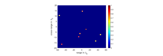
Figure 2: The true ${\mbox{\boldmath$\chi$}}=\mbox{diag}(X)=\mbox{diag}(\mbox{\boldmath$\rho$}\,\mbox{\boldmath$\rho$}^{*})$, i.e., the absolute values squared of the point sources amplitudes.. The dimension of the image is $K=1681$.

In the following examples, we consider imaging of $M=8$ point sources; see Fig. 2. Instead of the $N^{2}$ cross-correlated data which are, in principle, available, we only use $\mathcal{N}=21N$ cross-correlated data picked at random. This reduces even more the dimensionality of the problem we solve. In Fig. 3, we present the results when the used data is noise-free. The left column shows the results when we use the $\ell_{1}$ algorithm (34); the top plot is the recovered image and the bottom plot the recovered ${\mbox{\boldmath$\chi$}}=\mbox{diag}(X)=\mbox{diag}(\mbox{\boldmath$\rho$}\,\mbox{\boldmath$\rho$}^{*})$ vector. The support of the sources is exact but the amplitudes are not. If it is important for an application to recover the amplitudes with precision, one can consider in a second step the full problem (15) for $\mbox{vec}(X)$ with all the interference terms $\rho_{k}\rho^{*}_{k^{\prime}}$ for $k\neq k^{\prime}$, but restricted to the exact support found in the first step. If there is no noise in the data, this second step finds the exact values of the amplitudes efficiently using an $\ell_{2}$ minimization method; see the right column of Fig. 3.

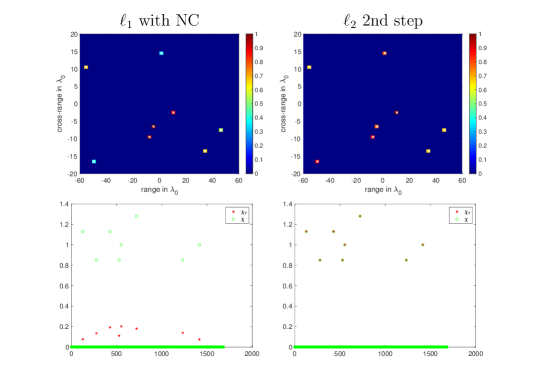
Figure 3: Imaging $M=8$ sources using correlations and the NC. The dimension of the image is $K=1681$. The dimension of the linear data is $N=441$. The $\ell_{1}$ images are obtained using $21N$ of the $N^{2}$ correlation data. Noise free data.

In Figs. 4 and 5 we consider the same configuration of sources but we add white Gaussian noise to the data. The resulting SNR values are $10$dB and $0$dB, respectively. In both cases, the solutions obtained in the first step look very similar to the one obtained in Fig. 3 for noise free data. This is so, because the noise in the data is dominated by the neglected interference terms. The actual effect of the additive noise is only seen in the 2nd step when we solve for $\mbox{vec}(X)$, restricted to the support, using an $\ell_{2}$ minimization method. Indeed, when the data are noisy we cannot recover the exact values of the amplitudes. Still, since an $\ell_{2}$ method is used on the correct support, the reconstructions are extremely robust and give very good results, even when the SNR is $0$dB.

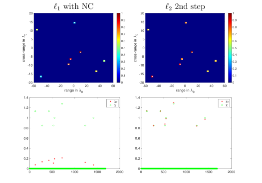
Figure 4: Imaging $M=8$ sources using correlations and the NC. The dimension of the image is $K=1681$. The dimension of the linear data is $N=441$. The $\ell_{1}$ images are obtained using $21N$ of the $N^{2}$ correlation data. Data with 10dB SNR.

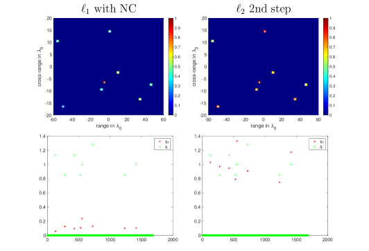
Figure 5: Imaging $M=8$ sources using correlations and the NC. The dimension of the image is $K=1681$. The dimension of the linear data is $N=441$. The $\ell_{1}$ images are obtained using $21N$ of the $N^{2}$ correlation data. Data with 0dB SNR.

To illustrate the robustness of the reconstructions of the entire matrix $X=\mbox{\boldmath$\rho$}\,\mbox{\boldmath$\rho$}^{*}$ we also plot in Fig. 6 the angle of $X_{\tau}$ compared to the angle of $X$ restricted on the support recovered during the first step. We get an exact reconstruction for noise-free data. The error in the reconstruction increases as the SNR decreases but the results are very satisfactory even for the $0$dB SNR case.

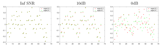
Figure 6: Imaging $M=8$ sources using correlations and the NC. The dimension of the image is $K=1681$. The dimension of the linear data is $N=441$. The angle of the components of $X_{\tau}$ compared to angle of the components of the true $X$ restricted on the support.

Again, the big advantage of the proposed $\ell_{1}$ minimization approach that seeks only for the components of $\mbox{diag}(X)$, and uses a Noise Collector to absorb the interference terms that are treated as noise, is that it is linear in the number of pixels $K$ instead of quadratic. This allows us to consider large scale problems. Moreover, as we observed in the results of Figs. 3 to 6, the number of data $\mathcal{N}$ used to recover the images do not need to be $N^{2}$, but only a multiple of $N$.

In Fig. 7 we illustrate the performance of the proposed $\ell_{1}$ approach for different sparsity levels $M$ and data sizes $\mathcal{N}$. There is no additive noise added to the data in this figure. Success in recovering the true support of the unknown $\chi$ corresponds to the value $1$ (yellow) and failure to $0$ (blue). The small phase transition zone (green) contains intermediate values. The red line is the the estimate $\sqrt{\mathcal{N}}/(2\sqrt{\ln\mathcal{N}})$. These results are obtained by averaging over 10 realizations.

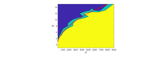
Figure 7: Algorithm performance for exact support recovery during the first step using $\ell_{1}$ and the Noise Collector. Success corresponds to the value $1$ (yellow) and failure to $0$ (blue). The small phase transition zone (green) contains intermediate values. The red line is the estimate $\sqrt{\mathcal{N}}/(2\sqrt{\ln\mathcal{N}})$. Ordinate and abscissa are the data used $\mathcal{N}$ and the sparsity $M$.

6 Conclussions

In this paper, we consider the problem of sparse signal recovery from cross correlation measurements. The unknown in this case is the correlated matrix signal $X=\mbox{\boldmath{$\rho$}}\mbox{\boldmath{$\rho$}}^{*}$ whose dimension grows quadratically with the size $K$ of $\rho$ and, hence, inversion becomes computationally unfeasible as $K$ increases. To overcome this issue, we propose a novel dimension reduction approach. Specifically, we vectorize the problem and consider as unknown only the diagonal terms $|\rho_{i}|^{2}$ of $X$ whose dimension is $K$ and are related to the data through a linear transformation. The off-diagonal interfernce terms $\rho_{i}\rho^{*}_{j}$ for $i\neq j$ are treated as noise and are absorbed using the Noise Collector approach introduced in [17]. This allows us to recover the signal exactly using efficient $\ell_{1}$-minimization algorithms. The cost of solving this dimension reduced problem is similar to the one using linear data. Furthermore, our numerical experiments show that the suggested approach is robust with respect to additive noise in the data. Finally, we point out that when using cross correlated data the maximum level of sparsity that can be recovered increases to $O(N/\sqrt{\ln N})$ instead of $O(\sqrt{N}/\sqrt{\ln N})$ for the linear data.

Appendix A Proofs of the Theorems

A.1 Proof of Theorem 2

Proof:

To prove the first claim, we repeat the proof of Theorem 2 from [17]. Define $H_{1}$ as the convex hull of the columns of ${\cal C}$, and $H_{2}$ as the convex hull of the columns $\mbox{\boldmath{$t$}}_{i}$ of $T$ in the support of $\chi$, as follows.

$$H_{1}=H_{1}(\tau)=\left\{x\in\mathbb{R}^{N}\left|x=\tau\sum_{i=1}^{\Sigma}\xi_{i}\mbox{\boldmath{$c$}}_{i},~{}\sum_{i=1}^{\Sigma}|\xi_{i}|\leqslant 1\right.\right\},$$

$$H_{2}=\left\{x\in\mathbb{R}^{N}\left|x=\sum_{i\in\mbox{supp}(\mbox{\boldmath{$\chi$}})}\xi_{i}\mbox{\boldmath{$t$}}_{i},~{}\sum_{i=1}^{K}|\xi_{i}|\leqslant 1\right.\right\},$$

and

$$H(\tau)=\left\{\xi h_{1}+(1-\xi)h_{2},0\leqslant\xi\leqslant 1,h_{i}\in H_{i}\right\}.$$

Suppose the $(M+1)$-dimensional space $V$ is spanned by $e$ and the column vectors $\mbox{\boldmath{$t$}}_{j}$, with $j$ in the support of $\chi$. Denote by $\mbox{\boldmath{$t$}}_{i}^{v}$ the orthogonal projections of $\mbox{\boldmath{$t$}}_{i}$ on $V$. We will prove that $\mbox{supp}(\mbox{\boldmath{$\chi$}}_{\tau})\subset\mbox{supp}(\mbox{\boldmath{$\chi$}})$ if for any $\mbox{\boldmath{$t$}}_{j}$, $j\not\in\mbox{supp}(\mbox{\boldmath{$\chi$}})$, we have $\mbox{\boldmath{$t$}}^{v}_{j}\subset H(\tau)$ strictly (i.e. $\mbox{\boldmath{$t$}}^{v}_{j}\cap\partial H(\tau)=\emptyset$) Fix $j\not\in\mbox{supp}(\mbox{\boldmath{$\chi$}})$, and suppose

$$\mbox{\boldmath{$t$}}^{v}_{j}=\xi_{0}\mbox{\boldmath{$t$}}_{0}+\sum_{k=1}^{M}\xi_{k}\mbox{\boldmath{$t$}}_{i_{k}},\mbox{ where all }i_{k}\in\mbox{supp}(\mbox{\boldmath{$\chi$}}),\mbox{\boldmath{$t$}}_{0}=\frac{\mbox{\boldmath{$e$}}}{\|\mbox{\boldmath{$e$}}\|}.$$ (35)

Suppose $|\xi_{k}|=\max_{n\leqslant M}|\xi_{n}|$. Multiply (35) by $|\xi_{k}|\mbox{\boldmath{$t$}}^{v}_{k}/\xi_{k}$. Using (22) and (23) we obtain

$$c_{0}\frac{\sqrt{\ln{\cal N}}}{\sqrt{\cal N}}\geqslant|\xi_{k}|\left(1-Mc_{0}\frac{\sqrt{\ln{\cal N}}}{\sqrt{\cal N}}\right)$$

Choose $\alpha$ in (24) so that

$$Mc_{0}\frac{\sqrt{\ln{\cal N}}}{\sqrt{\cal N}}\leqslant\frac{1}{4}.$$ (36)

Then,

$$\left(1-Mc_{0}\frac{\sqrt{\ln{\cal N}}}{\sqrt{\cal N}}\right)\geqslant\frac{3}{4},$$

and therefore,

$$|\xi_{k}|\leqslant\frac{4c_{0}}{3}\frac{\sqrt{\ln{\cal N}}}{\sqrt{\cal N}}$$

for all $k=0,1,2,\dots,M$. Hence, $\sum_{k=1}^{M}|\xi_{k}|\leqslant 1/3$. By the Milman’s extension of the Dvoretzky’s theorem [15] we can find $\tau_{0}=O(1)$ so that

$$4c_{0}\frac{\sqrt{\ln{\cal N}}}{\sqrt{\cal N}}\mbox{\boldmath{$t$}}_{0}:=\tilde{\mbox{\boldmath{$t$}}}_{0}\in H_{1}(\tau_{0})$$

with probability $1-1/{\cal N}^{\kappa}$. Therefore,

$$\!\!\!\!\!\!\!\!\!\!\!\!\!\!\!\!\!\!\!\!\!\!\!\!\!\!\!\!\!\!\!\!\mbox{\boldmath{$t$}}^{v}_{j}=\tilde{\xi}_{0}\tilde{\mbox{\boldmath{$t$}}}_{0}+\sum_{k=1}^{M}\xi_{k}\mbox{\boldmath{$t$}}_{i_{k}},\mbox{ where all }i_{k}\in\mbox{supp}(\mbox{\boldmath{$\chi$}})\,\mbox{ and }|\tilde{\xi_{0}}|+\sum_{k=1}^{M}|\xi_{k}|\leqslant 1/3+1/3\leqslant 2/3$$

and $\tilde{\mbox{\boldmath{$t$}}}_{0}\in H_{1}(\tau)$ for all $\tau\geqslant\tau_{0}$. Therefore, $\mbox{\boldmath{$t$}}^{v}_{j}\subset H(\tau)$ strictly.

To prove the second claim, we repeat the proof of Theorem 3 from [17]. Estimate (36) implies we can assume $\langle\mbox{\boldmath{$t$}}_{i},\mbox{\boldmath{$t$}}_{j}\rangle=0$ for $i\neq j$, $i,j\in\mbox{supp}(\mbox{\boldmath{$\chi$}})$ - this will only replace the constant $c_{1}$ in (26) to $2c_{1}/\sqrt{3}$ at most. Suppose $V^{i}$ are the $2$-dimensional spaces spanned by $e$ and $\mbox{\boldmath{$t$}}_{i}$ for $i\in\mbox{supp}(\mbox{\boldmath{$\chi$}})$. By the Milman’s extension of the Dvoretzky’s theorem [15] all $\lambda H(\tau)\cap V^{i}$ look like rounded rhombi depicted on Fig. 8, and $\lambda H_{1}(\tau)\cap V^{i}\subset B^{i}_{\lambda\tau}$ with probability $1-N^{-\kappa}$, where $B^{i}_{\lambda\tau}$ is a 2-dimensional $\ell_{2}$-ball of radius $\lambda\tau c_{0}\sqrt{\ln{\cal N}}/\sqrt{\cal N}$. Thus $\lambda H(\tau)\cap V^{i}\subset H^{i}_{\lambda\tau}$ with probability $1-N^{-\kappa}$, where $H^{i}_{\lambda\tau}$ is the convex hull of $B^{i}_{\lambda\tau}$ and a vector $\lambda\mbox{\boldmath{$f$}}_{i}$, $\mbox{\boldmath{$f$}}_{i}=\chi_{i}\|\mbox{\boldmath{$\chi$}}\|^{-1}_{\ell_{1}}\mbox{\boldmath{$t$}}_{i}$. Then $\mbox{supp}(\mbox{\boldmath{$\chi$}}_{\tau})=\mbox{supp}(\mbox{\boldmath{$\chi$}})$, if there exists $\lambda_{0}$ so that $\chi_{i}\mbox{\boldmath{$t$}}_{i}+\mbox{\boldmath{$e$}}$ lies on the flat boundary of $H^{i}_{\lambda_{0}}$ for all $i\in\mbox{supp}(\mbox{\boldmath{$\chi$}})$.

Figure 8: An intersection of $H(\tau)$ with the span$(\mbox{\boldmath{$t$}}_{i},\mbox{\boldmath{$e$}})$ is a rounded rhombus.

If $\min_{i\in\mbox{supp}(\mbox{\boldmath{$\chi$}})}|\chi_{i}|\geqslant\gamma\|\mbox{\boldmath{$\chi$}}\|_{\infty}$, then there exists a constant $c_{2}=c_{2}(\gamma)$ such that if $\chi_{i}\mbox{\boldmath{$t$}}_{i}+\mbox{\boldmath{$e$}}$ lies on the flat boundary of $H^{i}_{\lambda}$ for some $i$ and some $\lambda$, then there exists $\lambda_{0}$ so that $\chi_{i}\mbox{\boldmath{$t$}}_{i}+c_{2}\mbox{\boldmath{$e$}}$ lies on the flat boundary of $H^{i}_{\lambda_{0}}$ for all $i\in\mbox{supp}(\mbox{\boldmath{$\chi$}})$. If

$$\frac{|\langle\mbox{\boldmath{$t$}}_{i},\chi_{i}\mbox{\boldmath{$t$}}_{i}+\mbox{\boldmath{$e$}}\rangle|}{\|\chi_{i}\mbox{\boldmath{$t$}}_{i}+\mbox{\boldmath{$e$}}\|_{\ell_{2}}}\geqslant\frac{\tau c_{0}\sqrt{\ln{\cal N}}}{\sqrt{\cal N}\|\mbox{\boldmath{$f$}}_{i}\|_{\ell_{2}}}=\frac{\tau c_{0}\|\mbox{\boldmath{$\chi$}}\|_{\ell_{1}}\sqrt{\ln{\cal N}}}{\sqrt{\cal N}|\chi_{i}|},$$ (37)

then $\chi_{i}\mbox{\boldmath{$t$}}_{i}+c_{2}\mbox{\boldmath{$e$}}$ lies on the flat boundary of $H^{i}_{\lambda}$.

Since $|\langle\mbox{\boldmath{$t$}}_{i},\chi_{i}\mbox{\boldmath{$t$}}_{i}+\mbox{\boldmath{$e$}}\rangle|\geqslant|\chi_{i}|/2$ by (25), inequality (37) holds if

$$\frac{|\chi_{i}|}{\|\chi_{i}\mbox{\boldmath{$t$}}_{i}+\mbox{\boldmath{$e$}}\|_{\ell_{2}}}\geqslant\frac{2\tau c_{0}\|\mbox{\boldmath{$\chi$}}\|_{\ell_{1}}\sqrt{\ln{\cal N}}}{\sqrt{\cal N}|\chi_{i}|}.$$

By (26) and using $\|\mbox{\boldmath{$\chi$}}\|_{\ell_{1}}\leqslant M$ the last inequality is true if

$$M\leqslant\frac{\sqrt{\cal N}}{\tau c_{1}c_{0}\sqrt{\ln{\cal N}}}.$$

The last inequality is true if $\alpha$ in (24) is small enough. Thus, $\mbox{supp}(\mbox{\boldmath{$\chi$}}_{\tau})=\mbox{supp}(\mbox{\boldmath{$\chi$}})$. $\square$

A.2 Proof of Theorem 3

Proof:

We need to verify that all conditions of Theorem 2 are satisfied. Choose $c_{0}$, $\tau_{0}$, ${\cal N}_{0}$ and $\alpha$ so that Theorem 2 is satisfied with probability $1-\frac{1}{3{\cal N}^{\kappa}}$. Note that we can increase $c_{0}$, $\tau_{0}$, ${\cal N}_{0}$ and decrease $\alpha$ in this proof if necessary. We denote by $({\bar{\cal A}}\otimes{\cal A})_{k,l}$ the column of ${\bar{\cal A}}\otimes{\cal A}$ that arises from a tensor product $\bar{\mbox{\boldmath{$a$}}}_{k}\otimes\mbox{\boldmath{$a$}}_{l}$. If we use all $N^{2}$ of the data the columns ${\bar{\cal A}}\otimes{\cal A}$,then

$$\!\!\!\!\!\!\!\!\!\!\!\!\langle({\bar{\cal A}}\otimes{\cal A})_{k,l},({\bar{\cal A}}\otimes{\cal A})_{m,n}\rangle=\sum_{i=1}^{N}\sum_{j=1}^{N}\bar{a}_{k,i}a_{l,j}a_{m,i}\bar{a}_{n,j}=\langle\mbox{\boldmath{$a$}}_{m},\mbox{\boldmath{$a$}}_{k}\rangle\langle\mbox{\boldmath{$a$}}_{l},\mbox{\boldmath{$a$}}_{n}\rangle.$$

In particular, all columns of ${\bar{\cal A}}\otimes{\cal A}$ have length $1$. Therefore,

$$\left|\langle\mbox{\boldmath{$t$}}_{i},\mbox{\boldmath{$t$}}_{j}\rangle\right|=\left|({\bar{\cal A}}\otimes{\cal A})_{i,i},({\bar{\cal A}}\otimes{\cal A})_{j,j}\right|=\left|\langle\mbox{\boldmath{$a$}}_{i},\mbox{\boldmath{$a$}}_{j}\rangle\right|^{2}\leqslant\frac{\Delta^{2}}{N},$$

and condition (23) is verified if we choose ${\cal N}_{0}$ large enough.

Now we obtain

$$\lambda_{1}M\leqslant\|\mbox{\boldmath{$e$}}\|_{\ell_{2}}\leqslant\lambda_{2}M$$ (38)

with high probability. Note that (38) implies (26) because $\gamma M\leqslant\|\mbox{\boldmath{$\chi$}}\|_{\ell_{1}}\leqslant M$. We write

$$\|\mbox{\boldmath{$e$}}\|^{2}_{\ell_{2}}=\|\mbox{\boldmath{$\chi$}}\|^{2}_{\ell_{1}}+2\|\mbox{\boldmath{$\chi$}}\|_{\ell_{1}}\Xi_{1}+\Xi_{2},$$

where

$$\Xi_{1}=\sum_{k,l,k\neq l}\bar{\rho}_{k}\rho_{l}\langle\mbox{\boldmath{$a$}}_{k},\mbox{\boldmath{$a$}}_{l}\rangle,$$ (39)

and

$$\Xi_{2}=\sum_{\scriptsize\mbox{all indices different}}\rho_{k}\bar{\rho}_{l}\bar{\rho}_{m}\rho_{n}\langle\mbox{\boldmath{$a$}}_{m},\mbox{\boldmath{$a$}}_{k}\rangle\langle\mbox{\boldmath{$a$}}_{l},\mbox{\boldmath{$a$}}_{n}\rangle.$$ (40)

By Hanson-Wright inequality (48)

$$\mathbb{P}\left(|\Xi_{1}|>t\right)\leqslant 2\exp\left(-\frac{t^{2}/32}{\|{\bf M}\|^{2}_{F}}\right)$$

where ${\bf M}$ is a matrix with components $|\rho_{k}\rho_{l}|\langle\mbox{\boldmath{$a$}}_{k},\mbox{\boldmath{$a$}}_{l}\rangle$, $\|{\bf M}\|_{F}$ is its Frobenius (Hilbert-Schmidt) norm. Since $|\langle\mbox{\boldmath{$a$}}_{k},\mbox{\boldmath{$a$}}_{l}\rangle|\leqslant\Delta/\sqrt{N}$, we obtain $\|{\bf M}\|_{F}\leqslant\Delta M/\sqrt{N}$ (in our set-up $\|\mbox{\boldmath{$\rho$}}\|_{\ell_{\infty}}=1$). Take $t=\gamma M/8\leqslant\|\mbox{\boldmath{$\chi$}}\|_{\ell_{1}}/8$ and obtain

$$\!\!\!\!\!\!\!\!\!\!\!\!\mathbb{P}\left(|\Xi_{1}|>\gamma M/8\right)\leqslant 2\exp\left(-cN\right),c=c(\gamma),$$

which is negligible for large $N$. Thus

$$|\Xi_{1}|\leqslant\frac{\|\mbox{\boldmath{$\chi$}}\|_{\ell_{1}}}{8}$$ (41)

with probability $1-2\exp\left(-cN\right)$. Observe that $\Xi_{2}=(\Xi_{1})^{2}-\Xi_{3}$, where

$$\Xi_{3}=\sum_{\scriptsize m=l\mbox{ or }k=n\mbox{ or both}}\rho_{k}\bar{\rho}_{l}\bar{\rho}_{m}\rho_{n}\langle\mbox{\boldmath{$a$}}_{m},\mbox{\boldmath{$a$}}_{k}\rangle\langle\mbox{\boldmath{$a$}}_{l},\mbox{\boldmath{$a$}}_{n}\rangle.$$

For $\Xi_{3}$ we can use a deterministic estimate:

$$|\Xi_{3}|\leqslant 2\frac{c^{2}_{0}M^{3}}{N}\leqslant c\alpha\frac{\|\mbox{\boldmath{$\chi$}}\|^{2}_{\ell_{1}}}{\sqrt{\ln N}}\leqslant\frac{\|\mbox{\boldmath{$\chi$}}\|^{2}_{\ell_{1}}}{16}.$$

For $(\Xi_{1})^{2}$ we use (41). Using the union bound, we obtain

$$\frac{1}{2}\|\mbox{\boldmath{$\chi$}}\|^{2}_{\ell_{1}}\leqslant\|\mbox{\boldmath{$e$}}\|^{2}_{\ell_{2}}\leqslant\frac{3}{2}\|\mbox{\boldmath{$\chi$}}\|^{2}_{\ell_{1}}$$ (42)

with probability $1-2\exp\left(-cN\right)$. Thus, (38) holds with probability $1-2\exp\left(-cN\right)$.

We will now prove (22). For $m\not\in\mbox{supp}(\mbox{\boldmath{$\chi$}})$, consider a random variable

$$\!\!\!\!\!\!\!\!\!\!\!\!\!\!\!\!\!\!\!\!\!\!\!\!\Theta_{m}=\langle\mbox{\boldmath{$t$}}_{m},\mbox{\boldmath{$e$}}\rangle=\sum_{k,l,k\neq l}\bar{\rho}_{k}\rho_{l}\langle\mbox{\boldmath{$t$}}_{m},({\bar{\cal A}}\otimes{\cal A})_{k,l}\rangle=\sum_{k,l,k\neq l}\bar{\rho}_{k}\rho_{l}\langle\mbox{\boldmath{$a$}}_{m},\mbox{\boldmath{$a$}}_{k}\rangle\langle\mbox{\boldmath{$a$}}_{m},\mbox{\boldmath{$a$}}_{l}\rangle.$$ (43)

We have

$$\left|\langle\mbox{\boldmath{$t$}}_{m},({\bar{\cal A}}\otimes{\cal A})_{k,l}\rangle\right|=\left|\langle\mbox{\boldmath{$a$}}_{m},\mbox{\boldmath{$a$}}_{k}\rangle\langle\mbox{\boldmath{$a$}}_{m},\mbox{\boldmath{$a$}}_{l}\rangle\right|\leqslant\frac{\Delta^{2}}{N}$$ (44)

if $m\neq k$, and $m\neq l$. If ${\bf M}$ is a matrix with components $|\rho_{k}\rho_{l}|\langle\mbox{\boldmath{$a$}}_{m},\mbox{\boldmath{$a$}}_{k}\rangle\langle\mbox{\boldmath{$a$}}_{m},\mbox{\boldmath{$a$}}_{l}\rangle$, then $\|{\bf M}\|_{F}\leqslant\Delta^{2}M/N$. Using (38) choose $t=c_{0}\frac{\sqrt{\ln N^{2}}}{N}\|\mbox{\boldmath{$e$}}\|_{\ell_{2}}>c_{0}\frac{\gamma}{2}\frac{M\sqrt{\ln N}}{N}$ in Hanson-Wright inequality (48) to obtain:

$$\!\!\!\!\!\!\!\!\!\!\!\!\!\!\!\!\!\!\!\!\!\!\!\!\!\!\!\!\!\mathbb{P}\left(|\Theta_{m}|>c_{0}\frac{\sqrt{\ln N^{2}}}{N}\|\mbox{\boldmath{$e$}}\|_{\ell_{2}}\right)\leqslant\mathbb{P}\left(|\Theta_{m}|>c_{0}\frac{\gamma}{2}\frac{M\sqrt{\ln N}}{N}\right)\leqslant 2\exp\left(-\frac{\gamma^{2}c^{2}_{0}\ln N}{128\Delta^{4}}\right).$$

Then (22) holds with probability $1-\frac{1}{3{\cal N}^{\kappa}}$ if $c_{0}$ is large enough.

We will now prove (25). For $m\in\mbox{supp}(\mbox{\boldmath{$\chi$}})$ decompose

$$\!\!\!\!\!\!\!\!\!\!\!\!\!\!\!\!\!\!\!\!\!\!\!\!\Theta_{m}=\langle\mbox{\boldmath{$t$}}_{m},\mbox{\boldmath{$e$}}\rangle=\Theta^{1}_{m}+\Theta^{2}_{m}$$

where

$$\Theta^{1}_{m}=\sum_{k,l,k\neq l,k\neq m,l\neq m}\bar{\rho}_{k}\rho_{l}\langle\mbox{\boldmath{$a$}}_{m},\mbox{\boldmath{$a$}}_{k}\rangle\langle\mbox{\boldmath{$a$}}_{m},\mbox{\boldmath{$a$}}_{l}\rangle$$

and

$$\Theta^{2}_{m}=\sum_{k,k\neq m}\left(\bar{\rho}_{m}\rho_{k}+\bar{\rho}_{k}\rho_{m}\right)\langle\mbox{\boldmath{$a$}}_{m},\mbox{\boldmath{$a$}}_{k}\rangle$$ (45)

The distribution of the random variable $\Theta^{1}_{m}$ has exactly the same behavior as $\Theta_{m}$ for $m\not\in\mbox{supp}(\mbox{\boldmath{$\chi$}})$. We therefore have

$$\!\!\!\!\!\!\!\!\!\!\!\!\!\!\!\!\!\!\!\!\!\!\!\!\mathbb{P}\left(|\Theta^{1}_{m}|>\frac{\gamma}{4}\|\chi\|_{\ell_{\infty}}\right)\leqslant 2\exp\left(-c\frac{N^{2}}{\Delta^{4}M^{2}}\right)\leqslant 2\exp(-\tilde{c}\ln N/\alpha^{2})\leqslant\frac{1}{6}\frac{1}{{\cal N}^{\kappa}},$$

by Hanson-Wright inequality 48 if $\alpha$ is small enough. . If $m=l$ (or $m=k$) then

$$\left|\langle\mbox{\boldmath{$t$}}_{m},({\bar{\cal A}}\otimes{\cal A})_{k,m}\rangle\right|=\left|\langle\mbox{\boldmath{$a$}}_{m},\mbox{\boldmath{$a$}}_{k}\rangle\right|\leqslant\frac{\Delta}{\sqrt{N}}.$$ (46)

If we condition on $\mbox{\boldmath{$\rho$}}_{m}$, then $\Theta^{2}_{m}$ is a sum of independent random variables. Therefore by Hoeffding’s inequality

$$\mathbb{P}\left(|\Theta^{2}_{m}|>t\right)\leqslant 2\exp\left(-c\frac{t^{2}}{b^{2}}\right),\mbox{ where }b^{2}\leqslant\frac{c^{2}_{0}M}{N}\leqslant\frac{\Delta^{2}\alpha}{\ln N}.$$

Choosing $t$ appropriately we obtain

$$\mathbb{P}\left(|\Theta^{2}_{m}|>\frac{\gamma}{4}\|\chi\|_{\ell_{\infty}}\right)\leqslant\frac{1}{6}\frac{1}{{\cal N}^{\kappa}}.$$

by choosing $\alpha$ small enough. Using the union bound we conclude that

$$\mathbb{P}\left(|\Theta_{m}|>\frac{\gamma}{2}\|\chi\|_{\ell_{\infty}}\right)\leqslant\frac{1}{3}\frac{1}{{\cal N}^{\kappa}}$$

for $m\in\mbox{supp}(\mbox{\boldmath{$\chi$}})$. Applying the union bound we conclude that conditions (25), (22) and estimates in Theorem 2 hold with probability $1-\frac{1}{{\cal N}^{\kappa}}$. This completes the proof. $\square$

Remark 1

The proof of Theorem 3 reveals why we had to assume (25) for $m\in\mbox{supp}(\mbox{\boldmath{$\chi$}})$. When $m\not\in\mbox{supp}(\mbox{\boldmath{$\chi$}})$ then $\langle\mbox{\boldmath{$t$}}_{m},\mbox{\boldmath{$e$}}\rangle$ is estimated in (43) using (44). When $m\in\mbox{supp}(\mbox{\boldmath{$\chi$}})$ then $\langle\mbox{\boldmath{$t$}}_{m},\mbox{\boldmath{$e$}}\rangle$ contains $\Theta^{2}_{m}$ given by (45). For $\Theta^{2}_{m}$ we cannot use (44), and we have to use a weaker estimate (46).

A.3 A deterministic version of Theorem 3

Theorem 4

Suppose $X$ is a solution of (15), $\mbox{\boldmath{$\chi$}}=\mbox{diag}(X)$ is $M$-sparse, $\mbox{\boldmath{$d$}}\in\mathbb{C}^{\cal N}$, ${\cal N}=N^{2}$, and $T=({\bar{\cal A}}\otimes{\cal A})_{\mbox{\boldmath{$\chi$}}}:\mathbb{C}^{\cal K}\to\mathbb{C}^{\cal N}$. Fix $\beta>1$, and draw $\Sigma={\cal N}^{\beta}$ columns for ${\cal C}$, independently, from the uniform distribution on $\mathbb{S}^{{\cal N}-1}$ and define $\gamma$ as in (18) and $\Delta$ as in (30). Then, for any $\kappa>0$, there are constants $\alpha=\alpha(\kappa,\gamma,\Delta)$, $\tau=\tau(\kappa,\beta)$, and ${\cal N}_{0}={\cal N}_{0}(\kappa,\beta,\gamma,\Delta)$ such that the following holds. If $M\leqslant\alpha\sqrt{N}$ and $\mbox{\boldmath{$\chi$}}_{\tau}$ is the solution (17), then $\mbox{supp}(\mbox{\boldmath{$\chi$}})=\mbox{supp}(\mbox{\boldmath{$\chi$}}_{\tau})$ for all ${\cal N}>{\cal N}_{0}$ with probability $1-1/{\cal N}^{\kappa}$.

Proof:

We need to verify that all conditions of Theorem 2 are satisfied non-probabilistically. Conditions (23) is already verified in the proof of Theorem 3 under even weaker assumptions than in Theorem 4. Therefore we only need to verify estimates (26), (25) and (22).

Since

$$\mbox{\boldmath{$e$}}=\sum_{k\neq l}\bar{\rho}_{k}\rho_{l}({\bar{\cal A}}\otimes{\cal A})_{k,l},$$

we have

$$\!\!\!\!\!\!\!\!\!\!\!\!\!\!\!\!\!\!\!\!\!\!\!\!\!\!\!\!\!\!\!\!\!\!\!\!\|\mbox{\boldmath{$e$}}\|^{2}_{\ell_{2}}\leqslant\frac{2\Delta}{\sqrt{N}}\sum_{\scriptsize{all~{}indices}}\chi_{k}\left|\rho_{m_{1}}\right|\left|\rho_{m_{2}}\right|+\frac{\Delta^{2}}{N}\sum_{\scriptsize{all~{}indices}}\left|\rho_{m_{1}}\right|\left|\rho_{m_{2}}\right|\left|\rho_{k_{1}}\right|\left|\rho_{k_{2}}\right|+\sum_{k,m}\chi_{k}\chi_{m}$$

$$\!\!\!\!\!\!\!\!\!\!\!\!\!\!\!\!\!\!\!\!\!\!\!\!\!\!\!\!\!\!\!\!\!\!\!\!\leqslant 2\Delta\alpha\|\mbox{\boldmath{$\chi$}}\|_{\ell_{1}}\|\mbox{\boldmath{$\rho$}}\|^{2}_{\ell_{2}}+\Delta^{2}\alpha^{2}\|\mbox{\boldmath{$\rho$}}\|^{4}_{\ell_{2}}+\|\mbox{\boldmath{$\chi$}}\|^{2}_{\ell_{1}}=(1+\Delta\alpha)^{2}\|\mbox{\boldmath{$\chi$}}\|^{2}_{\ell_{1}}.$$

Thus estimate (26) holds.

A non-probabilistic version of estimate (25) is as follows. For $m\in\mbox{supp}(\mbox{\boldmath{$\chi$}})$ we have

$$\!\!\!\!\!\!\!\!\!\!\!\!\!\!\!\!\!\!\!\!\!\!\!\!\left|\langle\mbox{\boldmath{$t$}}_{m},\mbox{\boldmath{$e$}}\rangle\right|=\left|\sum_{k,l,k\neq l}\bar{\rho}_{k}\rho_{l}\langle\mbox{\boldmath{$t$}}_{m},({\bar{\cal A}}\otimes{\cal A})_{k,l}\rangle\right|\leqslant 2\sum_{k,k\neq m}\left|\rho_{k}\right|\left|\rho_{m}\right|\left|\langle\mbox{\boldmath{$t$}}_{m},({\bar{\cal A}}\otimes{\cal A})_{k,m}\rangle\right|$$

$$\!\!\!\!\!\!\!\!\!\!\!\!\!\!\!\!\!\!\!\!\!\!\!\!+\sum_{k,l,k\neq l\neq m}\left|\rho_{k}\right|\left|\rho_{l}\right|\left|\langle\mbox{\boldmath{$t$}}_{m},({\bar{\cal A}}\otimes{\cal A})_{k,l}\rangle\right|\leqslant\frac{2\Delta}{\sqrt{N}}\sum_{k}\left|\rho_{k}\right|\left|\rho_{m}\right|+\frac{\Delta^{2}}{N}\sum_{k,l}\left|\rho_{k}\right|\left|\rho_{l}\right|$$

$$\!\!\!\!\!\!\!\!\!\!\!\!\!\!\!\!\!\!\!\!\!\!\!\!\leqslant\left(\frac{2\Delta M}{\sqrt{N}}+\frac{\Delta^{2}M^{2}}{N}\right)\|\mbox{\boldmath{$\rho$}}\|^{2}_{\ell_{\infty}}=\left(\frac{2\Delta M}{\sqrt{N}}+\frac{\Delta^{2}M^{2}}{N}\right)\|\mbox{\boldmath{$\chi$}}\|_{\ell_{\infty}}\leqslant\frac{\gamma}{2}\|\mbox{\boldmath{$\chi$}}\|_{\ell_{\infty}}.$$

if $\alpha$ is small enough.

We now obtain a lower bound on $\|\mbox{\boldmath{$e$}}\|_{\ell_{2}}$. For $\Xi_{1}$ and $\Xi_{2}$ in (39) and (40), respectively, we have

$$|\Xi_{1}|\leqslant\frac{\Delta M^{2}}{\sqrt{N}}\leqslant\Delta\alpha M,~{}~{}|\Xi_{2}|\leqslant\frac{\Delta^{2}M^{4}}{N}\leqslant\Delta^{2}\alpha^{2}M^{2}.$$

Since

$$\|\mbox{\boldmath{$e$}}\|^{2}_{\ell_{2}}=\|\mbox{\boldmath{$\chi$}}\|^{2}_{\ell_{1}}+2\|\mbox{\boldmath{$\chi$}}\|_{\ell_{1}}\Xi_{1}+\Xi_{2},\mbox{ and }\|\mbox{\boldmath{$\chi$}}\|_{\ell_{1}}=M$$

we can choose $\alpha$ so that

$$M/2=\|\mbox{\boldmath{$\chi$}}\|_{\ell_{1}}/2\leqslant\|\mbox{\boldmath{$e$}}\|^{2}_{\ell_{2}}.$$

To show (22) observe that

$$\left|\langle\mbox{\boldmath{$t$}}_{m},({\bar{\cal A}}\otimes{\cal A})_{k,l}\rangle\right|=\left|\langle\mbox{\boldmath{$a$}}_{m},\mbox{\boldmath{$a$}}_{k}\rangle\langle\mbox{\boldmath{$a$}}_{m},\mbox{\boldmath{$a$}}_{l}\rangle\right|\leqslant\Delta^{2}/N,$$

because $m\neq k$, and $m\neq l$. Therefore

$$\!\!\!\!\!\!\!\!\!\!\!\!\!\!\!\!\!\!\!\!\!\!\!\ \left|\langle\mbox{\boldmath{$t$}}_{m},\mbox{\boldmath{$e$}}\rangle\right|=\left|\sum_{k,l,k\neq l}\bar{\rho}_{k}\rho_{l}\langle\mbox{\boldmath{$t$}}_{m},({\bar{\cal A}}\otimes{\cal A})_{k,l}\rangle\right|\leqslant\frac{\Delta^{2}M^{2}}{N}\leqslant\frac{\Delta^{2}\alpha\|\mbox{\boldmath{$e$}}\|_{\ell_{2}}}{\sqrt{N}},$$

and (22) follows either for choosing $\alpha$ small or $\ln N$ large. $\square$

A.4 Hansen-Wright’s Inequality for bounded symmetric random variables

For simplicity of presentation all random variables here are real. Suppose $X_{i}$ are independent sub-gaussian random variables, $\mathbb{E}(X_{i})=0$, and the sub-gaussian norms $\|X_{i}\|_{\psi_{2}}\leqslant K$. Consider

$$\Xi=\sum_{i,j}X_{j}X_{i}m_{ij},$$

where $m_{ij}$ are entries of a deterministic $M\times M$ diagonal-free (i.e. $m_{ii}=0$) matrix ${\bf M}$. The Hanson-Wright inequality (see e.g. [18]) is

$$\mathbb{P}\left(|\Xi|>t\right)\leqslant 2\exp\left(-c\min\left(\frac{t^{2}}{K^{4}\|{\bf M}\|^{2}_{F}},\frac{t}{K^{2}\|{\bf M}\|}\right)\right)$$ (47)

where $\|{\bf M}\|_{F}$ is the Frobenius (Hilbert-Schmidt) norm of ${\bf M}$, and $\|{\bf M}\|$ is its operator norm. If we use this inequality in the proof of our Theorem 3, then the result becomes weaker than Theorem 1 by a factor of $\sqrt{\ln N}$ because in our setting

$$\min\left(\frac{t^{2}}{K^{4}\|{\bf M}\|^{2}_{F}},\frac{t}{K^{2}\|{\bf M}\|}\right)=\frac{t}{K^{2}\|{\bf M}\|}.$$

In order to obtain Theorem 3 in its present form, we need a slight strengthening of (47). Our proof is a modification of two proofs from [20] and [18]. It may already exist in the literature, but we were not able to find it. Therefore we provide it here for the reader’s convenience. We assume that our random variables are symmetric and bounded. This holds if a random variable is uniformly distributed on the (complex) unit circle as in Theorem 3.

Theorem 5

(Hansen-Wright inequality for bounded symmetric random variables) Suppose $X_{i}$ are independent symmetric random variables, with $\|X_{i}\|_{\ell_{\infty}}\leqslant K$. Let $\Xi=\sum_{i\neq j}X_{j}X_{i}m_{ij}$. Then

$$\mathbb{P}\left(|\Xi|>t\right)\leqslant 2\exp\left(-\frac{t^{2}/32}{K^{4}\|{\bf M}\|^{2}_{F}}\right).$$ (48)

Proof:

By replacing $X_{i}$ with $X_{i}/K$ we can assume $K=1$. By Chebyshev’s inequality

$$\mathbb{P}\left(\Xi>t\right)=\mathbb{P}\left(e^{\lambda\Xi}>e^{\lambda t}\right)\leqslant e^{-\lambda t}\mathbb{E}\left(e^{\lambda\Xi}\right)$$ (49)

for any $\lambda>0$. We now use decoupling. Consider independent Bernoulli random variables $\mu_{i}=0$ or $1$ with probability $1/2$. Since $\mathbb{E}(\mu_{i})(1-\mu_{j})=1/4$ for $i\neq j$ we conclude $\Xi=4\mathbb{E}_{\mu}\Xi_{\mu}$, where

$$\Xi_{\mu}=\sum_{i\neq j}\mu_{j}(1-\mu_{i})X_{j}X_{i}m_{ij},$$

and $\mathbb{E}_{\mu}$ is conditional expectation with respect to $\mu=(\mu_{1},\dots,\mu_{M})$. Using independence of $X=(X_{1},\dots,X_{M})$ and $\mu$, and applying Jensen’s inequality we obtain

$$\mathbb{E}\left(e^{\lambda\Xi}\right)=\mathbb{E}_{X}\left(e^{\lambda\Xi}\right)\leqslant\mathbb{E}_{X}\mathbb{E}_{\mu}\left(e^{4\lambda\Xi_{\mu}}\right)=\mathbb{E}_{\mu}\mathbb{E}_{X}\left(e^{4\lambda\Xi_{\mu}}\right)$$

where $\mathbb{E}_{X}$ is conditional expectation with respect to $X$. This implies there exist a realization of $\mu$ such that $\mathbb{E}_{X}\left(e^{\lambda\Xi}\right)\leqslant\mathbb{E}_{X}\left(e^{4\lambda\Xi_{\mu}}\right)$ for this $\mu$. Fix this $\mu$ and the corresponding set of indices $\Lambda_{\mu}=\{i|\delta_{i}=1\}$. Then we can write $\Xi_{\mu}=\sum_{i\neq j,i\in\Lambda_{\mu},j\in\Lambda^{c}_{\mu}}X_{j}X_{i}m_{ij}$. Since the random variables $X_{i}$, $i\in\Lambda_{\mu}$ and $X_{i}$, $i\in\Lambda^{c}_{\mu}$ are independent, their distribution will not change if we replace $X_{i}$, $i\in\Lambda^{c}_{\mu}$ by $X^{{}^{\prime}}_{i}$, $i\in\Lambda^{c}_{\mu}$, where $X^{{}^{\prime}}_{i}$ is an independent copy of $X_{i}$. In other words we have

$$\mathbb{E}_{X,X^{\prime}}\left(e^{\lambda\Xi}\right)\leqslant\mathbb{E}_{X}\left(e^{4\lambda\tilde{\Xi}_{\mu}}\right),\mbox{ where }\tilde{\Xi}_{\mu}=\sum_{i\neq j,i\in\Lambda_{\mu},j\in\Lambda^{c}_{\mu}}X^{{}^{\prime}}_{j}X_{i}m_{ij}.$$

We now claim that

$$\mathbb{E}_{X,X^{\prime}}\left(e^{4\lambda\tilde{\Xi}_{\mu}}\right)\leqslant\mathbb{E}_{X,X^{\prime}}\left(e^{4\lambda\tilde{\Xi}}\right),\mbox{ where }\tilde{\Xi}=\sum_{i\neq j}X^{{}^{\prime}}_{j}X_{i}m_{ij}.$$

Indeed, Lemma 6.1.2 in [20] states that $\mathbb{E}\left(F(Y)\right)\leqslant\mathbb{E}\left(F(Y+Z)\right)$ for any convex function $F$, if $Y$ and $Z$ are independent and $\mathbb{E}(Z)=0$. In our case we take $F(x)=e^{4\lambda x}$, $Y=\tilde{\Xi}_{\mu}$ and $Z=\tilde{\Xi}-\tilde{\Xi}_{\mu}$. If we condition on $X_{i}$, $i\in\Lambda_{\mu}$ and $X^{{}^{\prime}}_{i}$, $i\in\Lambda^{c}_{\mu}$, then $Y$ is fixed, $Z$ is independent $Y$ and its conditional expectation is zero. Hence the following decoupling estimate is obtained.

$$\mathbb{E}\left(e^{\lambda\Xi}\right)\leqslant\mathbb{E}\left(e^{4\lambda\tilde{\Xi}}\right),\mbox{ where }\tilde{\Xi}=\sum_{i\neq j}X^{{}^{\prime}}_{j}X_{i}m_{ij}.$$ (50)

By independence

$$\mathbb{E}\left(e^{4\lambda\tilde{\Xi}}\right)=\prod_{i\neq j}\mathbb{E}\left(e^{4\lambda m_{ij}X_{i}X^{{}^{\prime}}_{j}}\right).$$

Since random variables are symmetric

$$\!\!\!\!\!\!\!\!\!\!\!\!\!\!\!\!\!\!\!\!\!\!\!\!\!\!\!\!\!\!\!\!\!\mathbb{E}\left(e^{4\lambda m_{ij}X_{i}X^{{}^{\prime}}_{j}}\right)=\frac{1}{2}\mathbb{E}\left(e^{4\lambda m_{ij}\left|X_{i}X^{{}^{\prime}}_{j}\right|}+e^{-4\lambda m_{ij}\left|X_{i}X^{{}^{\prime}}_{j}\right|}\right)\leqslant\mathbb{E}\left(e^{8\lambda^{2}m^{2}_{ij}\left|X_{i}X^{{}^{\prime}}_{j}\right|^{2}}\right)\leqslant e^{8\lambda^{2}m^{2}_{ij}}.$$

Using the last two estimates in (50) we obtain

$$\mathbb{E}\left(e^{\lambda\Xi}\right)\leqslant e^{8\lambda^{2}\|{\bf M}\|_{F}^{2}}.$$

Plugging the lsat inequality in 49 and optimizing over $\lambda$ we obtain

$$\mathbb{P}\left(\Xi>t\right)\leqslant\inf_{\lambda>0}e^{-\lambda t+8\lambda^{2}\|{\bf M}\|_{F}^{2}}<e^{-\frac{t^{2}}{32\|{\bf M}\|_{F}^{2}}}.$$

$\square$

References

- [1] Beck, Amir, and Teboulle, Marc, A Fast Iterative Shrinkage-Thresholding Algorithm for Linear Inverse Problems, SIAM J. Img. Sci. 2 (2009), pp.183–202.
- [2] A. Bakulin and R. Calvert, The virtual source method: Theory and case study, Geophysics, 71 (2006), pp. SI139–SI150.
- [3] E. J. Candès, Y. C. Eldar, T. Strohmer, and V. Voroninski, Phase Retrieval via Matrix Completion, SIAM J. Imaging Sci. 6 (2013), pp. 199–225.
- [4] A. Chai, M. Moscoso and G. Papanicolaou, Array imaging using intensity-only measurements, Inverse Problems 27 (2011), 015005.
- [5] A. Chai, M. Moscoso and G. Papanicolaou, Imaging strong localized scatterers with sparsity promoting optimization, SIAM J. Imaging Sci. 10 (2014), pp. 1358–1387.
- [6] E. Daskalakis, C. Evangelidis, J. Garnier, N. Melis, G. Papanicolaou and C. Tsogka, Robust seismic velocity change estimation using ambient noise recordings, Geophys. J. Int. (2016).
- [7] J. Garnier and G. Papanicolaou, Passive Sensor Imaging Using Cross Correlations of Noisy Signals in a Scattering Medium, SIAM J. Imaging Sci. 2 (2009), pp. 396-437.
- [8] J. Garnier and G. Papanicolaou, Role of scattering in virtual source imaging, SIAM Journal of Imaging Science 7 (2014), pp. 1210–1236.
- [9] J. Garnier and G. Papanicolaou, Passive imaging with ambient noise, Cambridge University Press, 2016.
- [10] J. Garnier, G. Papanicolaou, A. Semin, C. Tsogka, Signal to Noise Ratio Analysis in Virtual Source Array Imaging, SIAM Journal of Imaging Science 8 (2015), pp. 248–279.
- [11] R. M. Gray, Toeplitz and Circulant Matrices: A Review, Foundations and Trends in Communications and Information Theory 2 (2006), pp. 155–239.
- [12] P. R. Griffiths and J. A. De Haseth, Fourier Transform Infrared Spectrometry, John Wiley & Sons Inc., Hoboken, 2007.
- [13] T. Helin, M. Lassas, L. Oksanen, and T. Saksal, Correlation based passive imaging with a white noise source, Journal de Mathématiques Pures et Appliquées 116 (2018), pp. 132–160.
- [14] J. Laviada, A. Arboleya-Arboleya, Y. Alvarez-Lopez, C. Garcia-Gonzalez and F. Las-Heras, Phaseless synthetic aperture radar with efficient sampling for broadband near-field imaging: Theory and validation, IEEE Trans. Antennas Propag. 63 (2015), pp. 573–584.
- [15] V.D Milman, A new proof of A. Dvoretzky’s theorem on cross-sections of convex bodies, Funkcional. Anal. i Priložen. 5 (1971), pp. 28–37.
- [16] M. Moscoso, A. Novikov, G. Papanicolaou and L. Ryzhik, A differential equations approach to l1-minimization with applications to array imaging, Inverse Problems 28 (2012), 105001.
- [17] M. Moscoso, A. Novikov, G. Papanicolaou, C. Tsogka, The noise collector for sparse recovery in high dimensions, Proceedings of the National Academy of Science 117 (2020), pp. 11226–11232, doi: 10.1073/pnas.1913995117.
- [18] M. Rudelson, R. Vershynin, Hanson-Wright inequality and sub-gaussian concentration. Electron. Commun. Probab. 18 (2013), paper no. 82, 9 pp. doi:10.1214/ECP.v18-2865.
- [19] G. T. Schuster, Seismic Interferometry, Cambridge University Press, Cambridge, 2009.
- [20] R. Vershynin, High-dimensional probability. An introduction with applications in data science, Cambridge University Press, 2018.
- [21] K. Wapenaar, E. Slob, R. Snieder, and A. Curtis, Tutorial on seismic interferometry: Part 2 - Underlying theory and new advances, Geophysics, 75 (2010), pp. 75A211–75A227.