Optimization of loading factor preventing target cancellation

Abstract

Adaptive algorithms based on sample matrix inversion belong to an important class of algorithms used in radar target detection to overcome prior uncertainty of interference covariance. Sample matrix inversion problem is generally ill conditioned. Moreover, the contamination of the empirical covariance matrix by the useful signal leads to significant degradation of performance of this class of adaptive algorithms. Regularization, also known in radar literature as sample covariance loading, can be used to combat both ill conditioning of the original problem and contamination of the empirical covariance by the desired signal. However, the optimum value of loading factor cannot be derived unless strong assumptions are made regarding the structure of covariance matrix and useful signal penetration model. In this paper an iterative algorithm for loading factor optimization based on the maximization of empirical signal to interference plus noise ratio (SINR) is proposed. The proposed solution does not rely on any assumptions regarding the structure of empirical covariance matrix and signal penetration model. The paper also presents simulation examples showing the effectiveness of the proposed solution.

Index Terms—  adaptive filters, matrix inversion, interference suppression.

1 Introduction

Loading of the sample covariance matrix is used in loaded sample matrix inversion (LSMI) algorithm to alleviate losses incurred by using finite sample size estimate of the true covariance matrix [1]. The well known heuristic result due to Carlson [1] suggests fixing the value of loading factor at the level 10 dB above the white noise power. This choice of loading factor is indeed suitable in many practical scenarios. However, in some situations this value of loading factor might turn out to be too low, e.g., when useful signal is present in the training sample that is used for covariance matrix estimation. In this situation the effectiveness of LSMI using fixed loading factor significantly decreases. Moreover, if the signal power in training sample is sufficiently strong, target cancellation may occur. According to the well established methodology, loading factor can be optimized to prevent target cancellation by taking into account phased array calibration errors [2, 3]. This approach relies on a reasonably accurate model for training sample contamination. Often this model does not reflect the actual mechanisms that lead to the contamination of the training sample by the useful signal. For example, when the target is highly manoeuvring or distributed, this approach cannot model useful signal penetration. In this paper we concentrate on the non–parametric approach to loading factor optimization that does not rely on any model for training sample contamination. This approach is based on the iterative maximization of empirical Rayleigh quotient.

The remaining of this paper is organized as follows. Section 2 describes the LSMI algorithm and presents loading factor optimization problem. Section 3 describes the solution to the optimization problem and proposed iterative algorithm for the optimization of loading factor. Section 4 presents numerical examples showing the effectiveness of proposed algorithm. Finally, section 5 concludes the paper.

2 Problem Statement

The problem of finding optimum weights for the linear detector of a known signal ${\mathbf{s}}$ corrupted by the correlated interference with known covariance ${\mathbf{R}}$ can be formulated in terms of the output SINR maximization [3]:

$$\gamma_{\text{out}}=\frac{|{\mathbf{w}}^{H}{\mathbf{s}}|^{2}}{{\mathbf{w}}^{H}{\mathbf{R}}{\mathbf{w}}}.$$ (1)

Here $\gamma_{\text{out}}$ is the output SINR of the detector, also known as Rayleigh quotient, and ${\mathbf{w}}$ are detector weights. The expression for ${\mathbf{w}}$ maximizing (1) is known to have the following form [1]:

$${\mathbf{w}}_{\text{opt}}\propto{\mathbf{R}}^{-1}{\mathbf{s}}.$$ (2)

When ${\mathbf{R}}$ is not known in advance, one can resort to the adaptive version of (2) using the maximum likelihood estimate of covariance matrix [1]:

$$\widehat{\mathbf{R}}=\frac{1}{M}{\mathbf{X}}{\mathbf{X}}^{H},$$ (3)

instead of the true ${\mathbf{R}}$. Here ${\mathbf{X}}=[{\mathbf{x}}_{1},{\mathbf{x}}_{2},\ldots,{\mathbf{x}}_{M}]$ is a training sample containing $N\times 1$ vectors of the space–time samples $\{{\mathbf{x}}_{i}\}_{i=1}^{M}$ of locally homogeneous correlated Gaussian interference derived from a set of cells surrounding the cell of interest, $N$ is the dimensionality of space–time processing and $M$ is the number of training samples. The introduction of loading factor $\alpha$ leads to the following expression for the regularized estimate of the interference covariance matrix:

$$\widehat{\mathbf{R}}^{\prime}=\widehat{\mathbf{R}}+\alpha{\mathbf{I}},$$ (4)

leading to the adaptive LSMI algorithm:

$$\widehat{\mathbf{w}}\triangleq{\mathbf{w}}_{\text{LSMI}}=\left(\widehat{\mathbf{R}}+\alpha{\mathbf{I}}\right)^{-1}{\mathbf{s}}.$$ (5)

Given the structure (5) imposed on the estimator of optimum weights and the fact that optimum $\alpha$ is unknown, the following optimization problem can be stated:

$$\widehat{\alpha}_{\text{opt}}=\arg\max\limits_{\alpha}\widehat{\gamma}_{\text{out}}$$ (6)

Here we introduce $\widehat{\gamma}_{\text{out}}$ to clarify our assumption that $\widehat{\mathbf{w}}$ defined in (5) and $\widehat{\mathbf{R}}^{\prime}$ defined in (4) can be used to approximate $\gamma_{\text{out}}$ by the empirical SINR $\widehat{\gamma}_{\text{out}}$ while maximizing $\gamma_{\text{out}}$ with respect to $\alpha$.

3 Loading Factor Optimization

In the following we consider solving the problem (6). At first, we use the expression (1) for the true $\gamma_{\text{out}}$ to reformulate the problem. After that, we use the necessary approximations to arrive at the expression for the cost function.

1. Covariance matrix estimation $\widehat{\mathbf{R}}=\frac{1}{M}{\mathbf{X}}{\mathbf{X}}^{H}$    (3); 2. Initialization of iterative algorithm $\alpha_{1}=\sigma^{2}_{n}$; 3. For all $i=1\ldots T$ $\widetilde{\mathbf{w}}_{i}=\left(\widehat{\mathbf{R}}+\alpha_{i}{\mathbf{I}}\right)^{-1}{\mathbf{s}}$    (11); $\widetilde{\mathbf{v}}_{i}=\left(\widehat{\mathbf{R}}+\alpha_{i}{\mathbf{I}}\right)^{-1}\widetilde{\mathbf{w}}_{i}$    (11); $\lambda_{i}=-1-\frac{{2\widetilde{\mathbf{w}}_{i}^{H}\widetilde{\mathbf{v}}_{i}(1-\widetilde{\mathbf{w}}_{i}^{H}{\mathbf{s}})+\widetilde{\mathbf{w}}_{i}^{H}\widetilde{\mathbf{w}}_{i}\widetilde{\mathbf{v}}_{i}^{H}{\mathbf{s}}}}{{|{\mathbf{s}}^{H}\widetilde{\mathbf{v}}_{i}|^{2}}}$    (16); $\alpha_{i+1}=\frac{{\widetilde{\mathbf{w}}_{i}^{H}\widetilde{\mathbf{w}}_{i}+\widetilde{\mathbf{v}}_{i}^{H}{\mathbf{s}}+\lambda_{i}\widetilde{\mathbf{v}}_{i}^{H}{\mathbf{s}}}}{({2\widetilde{\mathbf{v}}_{i}^{H}\widetilde{\mathbf{w}}_{i}})}$    (15); 4. Estimation of weight vector $\widehat{\mathbf{w}}=\left(\widehat{\mathbf{R}}+\alpha_{T}{\mathbf{I}}\right)^{-1}{\mathbf{s}}$    (5);

Fig. 1: Iterative algorithm for estimation of loading factor $\alpha$ and weight vector $\widehat{\mathbf{w}}$.

To facilitate algebraic manipulations, the problem of maximizing $\gamma_{\text{out}}$ in (1) with respect to $\alpha$ can be reformulated in terms of minimizing ${\mathbf{w}}^{H}{\mathbf{R}}{\mathbf{w}}$ subject to a constraint on $|{\mathbf{w}}^{H}{\mathbf{s}}|^{2}$:

$$\alpha_{\text{opt}}=\arg\min\limits_{\alpha}{\mathbf{w}}^{H}{\mathbf{R}}{\mathbf{w}},\text{\ \ s. t.\ \ }|{\mathbf{w}}^{H}{\mathbf{s}}|^{2}=1$$ (7)

To resolve (7) we apply approximations ${\mathbf{w}}\simeq\widehat{\mathbf{w}}$ and ${\mathbf{R}}\simeq\widehat{\mathbf{R}}^{\prime}$ to ${\mathbf{w}}$ and ${\mathbf{R}}$ in (1) and use the linearization of (5) proposed in [4]. Note that $\alpha$ is small relative to the diagonal entries of $\widehat{\mathbf{R}}$ and we can use Taylor series to approximate (5) in the vicinity of the point $\alpha=0$:

$$\begin{split}\widehat{\mathbf{w}}&=\left[\widehat{\mathbf{w}}\right]_{\alpha=0}+\alpha\left[\frac{\partial}{\partial\alpha}\widehat{\mathbf{w}}\right]_{\alpha=0}+\frac{\alpha^{2}}{2!}\left[\frac{\partial^{2}}{\partial\alpha^{2}}\widehat{\mathbf{w}}\right]_{\alpha=0}\\ &+\frac{\alpha^{3}}{3!}\left[\frac{\partial^{3}}{\partial\alpha^{3}}\widehat{\mathbf{w}}\right]_{\alpha=0}+\ldots\end{split}$$ (8)

Calculating the first derivative of $\widehat{\mathbf{w}}$ with respect to $\alpha$:

$$\begin{split}\left[\frac{\partial}{\partial\alpha}\widehat{\mathbf{w}}\right]_{\alpha=0}&=\left[-\left(\widehat{\mathbf{R}}+\alpha{\mathbf{I}}\right)^{-1}{\mathbf{I}}\left(\widehat{\mathbf{R}}+\alpha{\mathbf{I}}\right)^{-1}{\mathbf{s}}\right]_{\alpha=0}\\ &=-\widehat{\mathbf{R}}^{-2}{\mathbf{s}},\end{split}$$ (9)

and limiting the expansion (8) to its first two components results in the following linear approximation of (5):

$$\widehat{\mathbf{w}}\simeq\widehat{\mathbf{R}}^{-1}{\mathbf{s}}-\alpha\widehat{\mathbf{R}}^{-2}{\mathbf{s}}.$$ (10)

The introduction of the notation

$$\widetilde{\mathbf{w}}\triangleq\widehat{\mathbf{R}}^{-1}{\mathbf{s}}\text{\ and \ }\widetilde{\mathbf{v}}\triangleq\widehat{\mathbf{R}}^{-1}\widetilde{\mathbf{w}}$$ (11)

leads to the representation of (10) in terms of $\widetilde{\mathbf{w}}$ and $\widetilde{\mathbf{v}}$

$$\widehat{\mathbf{w}}\simeq\widetilde{\mathbf{w}}-\alpha\widetilde{\mathbf{v}}.$$ (12)

Substituting (12) into (7) and using Lagrange multipliers results in the following cost function to be minimized:

$$\begin{split}J(\alpha)&=\widetilde{\mathbf{w}}^{H}{\mathbf{s}}-\alpha\widetilde{\mathbf{w}}^{H}\widetilde{\mathbf{w}}-\alpha\widetilde{\mathbf{v}}^{H}{\mathbf{s}}\\ &+\alpha^{2}\widetilde{\mathbf{v}}^{H}\widetilde{\mathbf{w}}+\lambda(\widetilde{\mathbf{w}}^{H}{\mathbf{s}}-\alpha\widetilde{\mathbf{v}}^{H}{\mathbf{s}}-1),\end{split}$$ (13)

where $\lambda$ is the Lagrange multiplier. The derivative of the cost function with respect to $\alpha$ has the following expression:

$$\frac{\partial}{\partial\alpha}J(\alpha)=-\widetilde{\mathbf{w}}^{H}\widetilde{\mathbf{w}}-\widetilde{\mathbf{v}}^{H}{\mathbf{s}}+2\alpha\widetilde{\mathbf{v}}^{H}\widetilde{\mathbf{w}}-\lambda\widetilde{\mathbf{v}}^{H}{\mathbf{s}}.$$ (14)

Equating (14) to zero we find the expression for $\widehat{\alpha}_{\text{opt}}$:

$$\widehat{\alpha}_{\text{opt}}=\frac{\widetilde{\mathbf{w}}^{H}\widetilde{\mathbf{w}}+\widetilde{\mathbf{v}}^{H}{\mathbf{s}}+\lambda\widetilde{\mathbf{v}}^{H}{\mathbf{s}}}{2\widetilde{\mathbf{v}}^{H}\widetilde{\mathbf{w}}}.$$ (15)

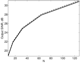
(a) Input SINR = 20 dB

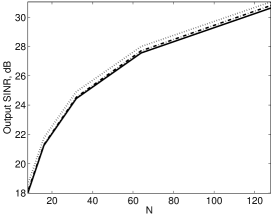
(b) Input SINR = 0 dB

(c) Input SINR = -20 dB

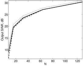
(d) Input SINR = -40 dB

(e) Input SINR = -60 dB

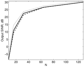
(f) Input SINR = -80 dB

Fig. 2: Output SINR of LSMI as a function of the number of samples $N$ for different values of input SINR. Dotted line denotes optimum algorithm with known covariance ${\mathbf{R}}$, solid line denotes proposed approach, dash–dotted line denotes LSMI with fixed loading factor $\alpha=10\sigma_{n}^{2}$ [1]. Training sample is not contaminated by the useful signal, $M=N$.

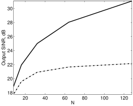
(a) Input SINR = 20 dB

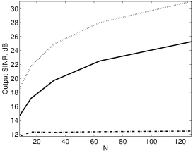
(b) Input SINR = 0 dB

(c) Input SINR = -20 dB

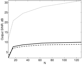
(d) Input SINR = -40 dB

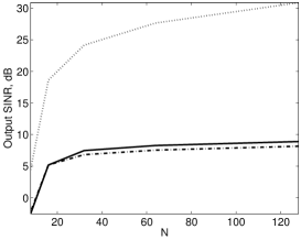
(e) Input SINR = -60 dB

(f) Input SINR = -80 dB

Fig. 3: Output SINR of LSMI as a function of the number of samples $N$ for different values of input SINR. Dotted line denotes optimum algorithm with known covariance ${\mathbf{R}}$, solid line denotes proposed approach, dash–dotted line denotes LSMI with fixed loading factor $\alpha=10\sigma_{n}^{2}$ [1]. Training sample is contaminated by the useful signal, $M=N$.

The expression for the unknown $\lambda$ follows from substituting (15) into constraint equation $|{\mathbf{w}}^{H}{\mathbf{s}}|^{2}=1$ following from (7):

$$\begin{split}\widehat{\mathbf{w}}^{H}{\mathbf{s}}&=(\widetilde{\mathbf{w}}^{H}-\widehat{\alpha}_{\text{opt}}^{*}\widetilde{\mathbf{v}}^{H}){\mathbf{s}}\\ &=\widetilde{\mathbf{w}}^{H}{\mathbf{s}}-\left(\frac{\widetilde{\mathbf{w}}^{H}\widetilde{\mathbf{w}}+\widetilde{\mathbf{v}}^{H}{\mathbf{s}}+\lambda\widetilde{\mathbf{v}}^{H}{\mathbf{s}}}{2\widetilde{\mathbf{v}}^{H}\widetilde{\mathbf{w}}}\right)^{*}\widetilde{\mathbf{v}}^{H}{\mathbf{s}}\\ &=\widetilde{\mathbf{w}}^{H}{\mathbf{s}}-\frac{\widetilde{\mathbf{w}}^{H}\widetilde{\mathbf{w}}\widetilde{\mathbf{v}}^{H}{\mathbf{s}}+{\mathbf{s}}^{H}\widetilde{\mathbf{v}}\widetilde{\mathbf{v}}^{H}{\mathbf{s}}+\lambda{\mathbf{s}}^{H}\widetilde{\mathbf{v}}\widetilde{\mathbf{v}}^{H}{\mathbf{s}}}{2\widetilde{\mathbf{w}}^{H}\widetilde{\mathbf{v}}}=1\end{split}$$

Finally, the expression for $\lambda$ becomes:

$$\lambda=-1-\frac{2\widetilde{\mathbf{w}}^{H}\widetilde{\mathbf{v}}(1-\widetilde{\mathbf{w}}^{H}{\mathbf{s}})+\widetilde{\mathbf{w}}^{H}\widetilde{\mathbf{w}}\widetilde{\mathbf{v}}^{H}{\mathbf{s}}}{|{\mathbf{s}}^{H}\widetilde{\mathbf{v}}|^{2}}$$ (16)

Thus the algorithm for data dependent $\alpha$ optimizaton, maximizing empirical SINR $\widehat{\gamma}_{\text{out}}$ consists of calculating $\widetilde{\mathbf{w}}$ and $\widetilde{\mathbf{v}}$ using (11) and $\lambda$ and $\widehat{\alpha}_{\text{opt}}$ using (16) and (15). Finally, $\widehat{\mathbf{w}}$ is calculated according to (5). Linear approximation in (10) prevents the convergence of the algorithm outlined above to $\widehat{\alpha}_{\text{opt}}$ during the first iteration if $\widehat{\alpha}_{\text{opt}}$ is comparatively large. We propose to use iterative algorithm to converge to this value. This algorithm is outlined in Fig. 1. Note that this algorithm is initialized with the value of $\alpha_{1}$ equal to the power of white noise $\sigma_{n}^{2}$. The idea behind this iterative algorithm is that at $i$–th iteration of the algorithm, $\widehat{\mathbf{w}}$ is expanded around the point $\alpha=\alpha_{i}$ and as $\alpha_{i}$ becomes closer to the true $\widehat{\alpha}_{\text{opt}}$ with growing $i$, the accuracy of approximation (12) increases leading to the convergence of the algorithm to $\widehat{\alpha}_{\text{opt}}$.

4 Numerical Examples

In this section we compare the performance of optimum algorithm with known covariance ${\mathbf{R}}$, LSMI with fixed loading factor $\alpha=10\sigma_{n}^{2}$ [1], and proposed approach to data–dependent estimation of $\alpha$ in terms of output SINR. Figures 2 and 3 show the results of this comparison. To generate these figures we used the following parameters of signal, noise and interference. Pulse repetition frequency was set to 20 kHz, interference consisted of two components with average Dopplers 0 and 1000 Hz and Doppler spread equal to 500 Hz, interference spectral envelope was Gaussian and input signal to white noise ratio was 10 dB. Doppler shift of the signal was 4 kHz, amplitude distribution of useful signal in training sample was Rayleigh and average power of signal in training sample (if present) was equal to its power in the cell of interest. The number of iterations $T$ in proposed algorithm was 3. The results were averaged over 500 Monte–Carlo trials.

Figure 2 shows output SINR of LSMI algorithm when training sample is not contaminated by the useful signal and Fig. 3 shows the results of training sample contamination. By observing these figures we can conclude that when useful signal is present in training sample, severe degradation of LSMI performance occurs if fixed loading factor is used. The algorithm using adaptive loading factor calculated using proposed approach is able to alleviate this effect, especially if useful signal dominates in the training sample. On the other hand, by observing Fig. 2 we can see that the introduction of adaptive loading factor leads to insubstantial loss in performance when useful signal is absent from the training sample. Thus we can conclude that the application of the proposed approach yields overall performance improvement when used in conjunction with LSMI algorithm. We can explain this result by the fact that the proposed algorithm tries to find a balance between the gain that is obtained by applying matched filter for white noise case ${\mathbf{w}}={\mathbf{s}}$ and the adaptive filter for colored noise case ${\mathbf{w}}=\widehat{\mathbf{R}}^{-1}{\mathbf{s}}$. In the situation when useful signal is not present in training sample, the application of the latter filter gives the best gain. Whereas when the training sample is contaminated by the useful signal, the application of this adaptive filter may actually lead to significant performance degradation due to signal cancellation effect. Thus in the latter situation the proposed algorithm automatically increases the loading factor so that more emphasis is put on non–adaptive weight vector ${\mathbf{w}}={\mathbf{s}}$. However, the observation of Fig. 3(e) and Fig. 3(f) leads to the conclusion that this loading factor tuning does not lead to significant performance improvement when interference is very strong. This can be attributed to the fact that in this case it is not possible to achieve performance improvement by just varying the effect of the two mentioned weight vectors.

5 Concluding Remarks

In this paper an iterative algorithm for loading factor optimization is proposed within the framework of LSMI algorithm. Linearization of the expression for weights obtained via LSMI algorithm is used to derive constrained empirical cost function. An expression for loading factor minimizing this cost function is derived. After that, an iterative solution is proposed to take into account the fact that the linearization prevents the convergence of the proposed algorithm during the first iteration. Finally, simulation examples showing the effectiveness of the proposed scheme along with the discussion of obtained results are presented. Analytical justification of the algorithm described in this paper is the subject to further development.

References

- [1] B. D. Carlson, “Covariance matrix estimation errors and diagonal loading in adaptive arrays,” IEEE Transactions on Aerospace and Electronic Systems, vol. 24, no. 4, pp. 397–401, Jul. 1988.
- [2] A. Beck and Y. C. Eldar, “Doubly constrained robust capon beamformer with ellipsoidal uncertainty sets,” IEEE Transactions on Signal Processing, vol. 55, no. 2, pp. 753–758, Jan. 2007.
- [3] S. A. Vorobyov, A. Gershman, and Z.-Q. Luo, “Robust adaptive beamforming using worst–case performance optimization: a solution to the signal mismatch problem,” IEEE Transactions on Signal Processing, vol. 51, no. 2, pp. 313–324, Feb. 2003.
- [4] Z. Tian, K. L. Bell, and H. L. Van Trees, “A Recursive Least Squares implementation for LCMP beamforming under quadratic constraint,” IEEE Transactions on Signal Processing, vol. 49, no. 6, pp. 1138–1145, Jun. 2001.