Pair the Dots: Jointly Examining Training History
and Test Stimuli for Model Interpretability

Abstract

Any prediction from a model is made by a combination of learning history and test stimuli. This provides significant insights for improving model interpretability: because of which part(s) of which training example(s), the model attends to which part(s) of a test example. Unfortunately, existing methods to interpret a model’s predictions are only able to capture a single aspect of either test stimuli or learning history, and evidences from both are never combined or integrated.

In this paper, we propose an efficient and differentiable approach to make it feasible to interpret a model’s prediction by jointly examining training history and test stimuli. Test stimuli is first identified by gradient-based methods, signifying the part of a test example that the model attends to. The gradient-based saliency scores are then propagated to training examples using influence functions Cook and Weisberg (1982); Koh and Liang (2017) to identify which part(s) of which training example(s) make the model attends to the test stimuli. The system is differentiable and time efficient: the adoption of saliency scores from gradient-based methods allows us to efficiently trace a model’s prediction through test stimuli, and then back to training examples through influence functions.

We demonstrate that the proposed methodology offers clear explanations about neural model decisions, along with being useful for performing error analysis, crafting adversarial examples and fixing erroneously classified examples.

1 Introduction

While neural models match or outperform the performance of state-of-the-art systems on a variety of tasks, they intrinsically suffer a severe shortcoming of being hard to explain (Simonyan et al., 2013; Bach et al., 2015a; Montavon et al., 2017; Kindermans et al., 2017). Unlike traditional feature-based classifiers that assign weights to human-interpretable features, neural network models operate like a black box with multiple layers non-linear operations on input representations (Glorot et al., 2011; He et al., 2016; Vaswani et al., 2017). The lack of interpretability not only significantly limits the scope of its applications in areas where model interpretations are essential, but also makes it hard to perform model behavior analysis and error analysis.

Any prediction from a model is made by a combination of learning history and test stimuli. To explain the prediction of a model, we need to answer the following question, because of which part(s) of which training example(s), the model attends to which part(s) of a test example. Unfortunately, existing strategies, test-focused methods Simonyan et al. (2013); Li et al. (2015a, 2016); Tenney et al. (2019); Clark et al. (2019); Wallace et al. (2019), and training-focused methods Koh and Liang (2017); Shafahi et al. (2018); Barham and Feizi (2019), only capture a single aspect, either test stimuli or learning history: Training-focused methods center on detecting the salient part of a test example that a model attends to, but are incapable of explaining why the model looks at the identified part. Training-focused methods identify influential training examples that hold responsible for a model’s prediction, but are incapable of explaining how the identified training examples affects a prediction. We thus need a model that can jointly examine training history and test stimuli.

The difficulty that hinders joint modeling lies at the algorithm level, where models for examining test stimuli are usually not differentiable with respect to the training examples, and that measuring the influence of a training example can also be time-intensive as it requires retraining the model. To overcome these difficulties, in this paper, we propose a differentiable model that can straightforwardly traces the prediction though test stimuli, and backs to training examples: Test stimuli is first identified using gradient-based methods, signifying the part of a test example that the model attends to. Next, the gradient-based saliency scores are propagated to training examples using influence functions Cook and Weisberg (1982); Koh and Liang (2017) to identify which part(s) of which training example(s) make the model attends to the test stimuli. The key advantages from the proposed system come in two folds: (1) the system is differentiable: the adoption of saliency scores from gradient-based methods are differentiable with respect to training examples through the influence function; (2) the system is time-efficient and the training model does not need to be retrained to examine learning history. In this way, we are able to efficiently trace a model’s prediction through test stimuli, and then back to training examples.

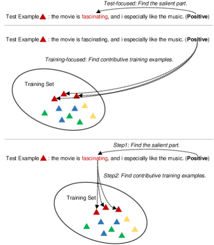
Figure 1: An illustration of different methods for interpreting neural decisions. Top: test-focused methods aim at finding the salient part of a given test example. Middle: training-focused methods associate training examples responsible for predicting a given test example. Bottom: the combination of both test-focused and training-focused methods extend beyond each of them, thereby giving more comprehensive explanations.

In summary, the contributions of this paper are as follows: (1) we propose an efficient and differentiable model that jointly examines training history and test stimuli for model interpretability; (2) we show that the proposed methodology is a versatile tool for a wide range of applications, including error analysis, crafting adversarial examples and fixing erroneously classified examples.

The rest of this work is organized as follows: in Section 2 we detail related work of test-focused and training-focused methods for model interpretations. The proposed model is described in Section 3. Experimental results are shown in Section 4, followed by a brief conclusion in Section 5.

2 Related Work

Test-focused interpretation methods aim at finding the most salient input features responsible for a prediction: Adler et al. (2018); Datta et al. (2016) explained neural models by perturbing various parts of the input, and compared the performance change in downstream tasks to measure feature importance; Ribeiro et al. (2016) proposed LIME, which interprets model predictions by approximating model predictions; Shrikumar et al. (2017) proposed DeepLIFT, which assigns each input a value to represent importance. Bach et al. (2015b) used Layer-Wise Relevance Propagation (LRP) to explain which pixels of an image are relevant for obtaining a model’s decision; Alvarez-Melis and Jaakkola (2017) presented a causal framework to explain structured models; Other methods include directly visualizing input features by computing saliency scores with gradients (Simonyan et al., 2013; Srinivas and Fleuret, 2019), using a surrogate model that learns to estimate the degree to which certain inputs cause outputs (Schwab and Karlen, 2019; Zhang et al., 2018), and selecting features that cause cell activations (Zeiler and Fergus, 2014; Springenberg et al., 2014; Kindermans et al., 2017) or signals through layers (Montavon et al., 2017; Sundararajan et al., 2017; Lundberg and Lee, 2017).

For training-focused methods, Koh and Liang (2017) used influence functions (Cook and Weisberg, 1982; Cook, 1986) to identify training points that are most responsible for a given prediction. A followup work from Han et al. (2020) finds that influence functions are particularly useful for tasks like natural language inference

In the context of NLP, methods for model interpretation include generating justifications to form interpretable summaries (Lei et al., 2016), studying the roles of vector dimensions (Shi et al., 2016), and analyzing hidden state dynamics in recurrent neural networks (Hermans and Schrauwen, 2013; Karpathy et al., 2015; Greff et al., 2016; Strobelt et al., 2016; Kádár et al., 2017). The attention mechanism has been used for model interpretation Jain and Wallace (2019); Serrano and Smith (2019); Wiegreffe and Pinter (2019); Vashishth et al. (2019). For example, Ghaeini et al. (2018) applied the attention mechanism to interpret models for the task of natural language inference; Vig and Belinkov (2019); Tenney et al. (2019); Clark et al. (2019) analyzed the attention structures inside self-attentions, and found that linguistic patterns emerge in different heads and layers.

A less relevant line of work is model poisoning, which manipulates the training process using poisoned data (Biggio et al., 2012; Mei and Zhu, 2015; Muñoz-González et al., 2017; Shafahi et al., 2018), or adversarial examples (Goodfellow et al., 2014; Kurakin et al., 2016; Moosavi-Dezfooli et al., 2016; Madry et al., 2017; Papernot et al., 2017; Athalye et al., 2018). It has been proven that training neural models with the combination of clean data and adversarial data can not only benefit test accuracy (Ebrahimi et al., 2017; Jia et al., 2019; Wang et al., 2020; Zhu et al., 2020; Zhou et al., 2020), but also offers explanations on the vulnerability of neural models (Miyato et al., 2016; Papernot et al., 2016; Zhao et al., 2017; Sato et al., 2018; Barham and Feizi, 2019).

3 Approach

Consider a task that maps an input $\mathbf{x}$ to a label $y$, where $\mathbf{x}$ is a list of tokens $\mathbf{x}=\{x_{1},x_{2},...,x_{N}\}$ and $L$ is the length of $\mathbf{x}$. Each token $x_{t}\in\mathbf{x}$ is associated with a $d$-dimensional word vector $\mathbf{e}_{i}$. The concatenation of $\mathbf{e}_{t}$ forms the $d\times L$ dimensional input embedding $\mathbf{E}$. A model takes as input $\mathbf{E}$, and maps it to single vector $\mathbf{h}_{x}$. $\mathbf{h}_{x}$ is next projected to a distribution over labels $\mathbf{y}$ using the softmax operator. In the following parts, we first introduce how to identify the salient feature of a test example,and then describe how to find training examples that are the most contributive to the selected salient token(s).

3.1 Detecting the Salient Part of a Test Example

To answer the question of the model attends to which part(s) of a given test example, we need to first decide which unit(s) of $\mathbf{E}$ make(s) the most significant contribution to $S_{y}(\mathbf{E})$, which is the probability of assigning label $y$ to $x$. Different widely used test-focused visualization methods can serve this purpose, such as LRP Bach et al. (2015b), LIME Ribeiro et al. (2016), DeepLIFT Shrikumar et al. (2017). But they can not serve our purpose since they are not differentiable with respect to training examples. We thus propose to use the gradient method Simonyan et al. (2013); Li et al. (2015a) because of the key advantage that it is differentiable and can thus be straightforwardly combined with the influence function to identify contributive training examples, as will be illustrated in the next subsection.

For the gradient-based model, since $S_{y}(\mathbf{E})$ is a highly non-linear function with respect to $\mathbf{E}$, we approximate it with a linear function of $\mathbf{e}$ by computing the first-order Taylor expansion:

$$S_{y}(\mathbf{e})\approx w_{y}(\mathbf{e})^{\top}\mathbf{e}+b$$ (1)

where $w_{y}(\mathbf{e})\in\mathbb{R}^{d\times 1}$ is the derivative of $S_{y}(\mathbf{E})$ with respect to the embedding $\mathbf{e}$:

$$w_{y}(\mathbf{e})=\nabla_{\mathbf{e}}S_{y}(\mathbf{E})$$ (2)

$w_{y}(\mathbf{e})$ the sensitiveness of the final decision to the change in one particular dimension, telling us how much word embedding dimensions contribute to the final decision. The saliency score is given by $w_{y}(\mathbf{e})$. Once we have the saliency score for each token embedding $\mathbf{e}_{i}$, we can accordingly select the salient tokens: we first sum up values of constituent dimensions in the word embedding and using $s(x_{t})=\sum_{j}w_{y}(\mathbf{e}_{t})_{j}$ as the saliency score for the token $x_{t}$. Next we can rank all constituent tokens $x_{t}$ by saliency scores to identify the token that a model attends to.

3.2 Training Examples’ Influence on the Detected Salient Parts

For each of the selected salient tokens $x_{t}$, we need to answer the question because of which part(s) of which training example(s), the model attends to $x_{t}$. Here we use the method of influence functions (Cook and Weisberg, 1982; Koh and Liang, 2017) for this purpose. The key idea of the influence function is to measure the change of the model’s parameters when a training point changes. Since the saliency score described in the previous subsection can be viewed as a function of the model’s parameters, the influence of changing of a training point on the saliency score can be straightforwardly computed through the chain rule.

Specifically, given training points $\{(\mathbf{x}_{i},y_{i})\}$, let $\theta\in\mathbb{R}^{P}$ be model parameters and $L(\mathbf{x}_{i},y_{i};\theta)$ be the loss, which is negative log likelihood. Let $z_{i}=(\mathbf{x}_{i},y_{i})$ for simplification. $\theta$ is learned by minimizing the loss given as follows:

$${\theta}=\arg\min_{\theta}\frac{1}{n}\sum_{z_{i}}L(z_{i};\theta)$$ (3)

The importance of $z_{i}$ is measured by the change of $\theta$ when $z_{i}$ is removed from the training set, given by: ${\theta}_{-z}-{\theta}$, where ${\theta}_{-z}\triangleq\arg\min_{\theta}\sum_{z_{i}:z_{i}\not=z}L(z_{i};\theta)$. But this is extremely computationally intensive since it requires retraining the model on the training set with $z_{i}$ removed. Fortunately, we can use influence functions Cook and Weisberg (1982); Koh and Liang (2017) to efficiently approximate the value. We define ${\theta}_{z,\epsilon}=\arg\min_{\theta}\frac{1}{n}\sum_{i=1}^{n}L(z_{i};\theta)+\epsilon L(z;\theta)$ to be the learned parameters when the loss function is upweighed by some small change $\epsilon$ on a training point $z$, and thus ${\theta}_{-z}$ is exactly ${\theta}_{z,-1}$. By leaving the proof to Appendix A, the influence of upweighting $z$ on $\theta$ (denoted by $I(z,{\theta})$) is given as follows:

$$I(z,{\theta})=\frac{\mathrm{d}{\theta}_{z,\epsilon}}{\mathrm{d}\epsilon}\Big{|}_{\epsilon=0}=-H^{-1}_{{\theta}}\nabla_{\theta}L(z;{\theta})$$ (4)

where $H_{{\theta}}=\frac{1}{n}\sum_{z_{i}}\nabla^{2}_{\theta}L(z_{i};{\theta})$ is the Hessian matrix. $H_{{\theta}}\in\mathbb{R}^{P\times P}$, where $\nabla^{2}_{\theta}L(z_{i};{\theta})=\frac{\partial^{2}L(z_{i};{\theta})}{\partial\theta_{i}\partial\theta_{j}}$. Using linear approximations, we can immediately get ${\theta}_{-z}-{\theta}\approx-\frac{1}{n}I(z,{\theta})$.

Our goal is to find the influence of a training example $z$ on a salient token $x_{t}$, i.e., the saliency score $w_{y}(\mathbf{e})$. Since $w_{y}(\mathbf{e})$ is a function of parameters ${\theta}$, we can apply the chain rule to measure the influence of $z_{i}$ on $w_{y}(\mathbf{e})$, denoted by $I(z,w_{y}(\mathbf{e}))$:

$$I(z,w_{y}(\mathbf{e})) \triangleq\frac{\mathrm{d}w_{y}(\mathbf{e};{\theta}_{z,\epsilon})}{\mathrm{d}\epsilon}\Big{|}_{\epsilon=0}$$ (5)

$$=\frac{\mathrm{d}w_{y}(\mathbf{e};{\theta}_{z,\epsilon})}{\mathrm{d}{\theta}_{z,\epsilon}}\frac{\mathrm{d}{\theta}_{z,\epsilon}}{\mathrm{d}\epsilon}\Big{|}_{\epsilon=0}$$

$$=-\nabla_{\theta}w_{y}(\mathbf{e})^{\top}H^{-1}_{{\theta}}\nabla_{\theta}L(z;{\theta})$$

Now for a given salient token $x_{t}$ with its word embedding $\mathbf{e}_{t}$, we are able to quantitatively measure the contribution of each training point $z_{i}$ on the detected salient part of the test exampled, quantified by $I(z_{i},w_{y}(\mathbf{e}))$.

Perturbing a Training Point

The above process describes how a training point can influence the model parameters. Further, we would like to measure how a perturbed training point can affect the model. Due to the discrete nature of NLP, an input example $\mathbf{x}=\{x_{1},x_{2},...,x_{t},...,x_{N}\}$ will be perturbed to $\tilde{\mathbf{x}}=\{x_{1},x_{2},...,x_{t}^{\prime},...,x_{N}\}$, with its constituent token $x_{t}$ altered to $\tilde{x}_{t}$. Concretely, for a training point $z=(\mathbf{x},y)$, we define its perturbed counterpart $\tilde{z}=(\tilde{\mathbf{x}},y)$. Let ${\theta}_{z,\tilde{z},\epsilon}\triangleq\arg\min_{\theta}\frac{1}{n}\sum_{i=1}^{n}L(z_{i};\theta)+\epsilon L(\tilde{z};\theta)-\epsilon L(z;\theta)$ be the parameters after substituting $z$ with $\tilde{z}$. Similar to Eq.4, the influence of changing $z$ to $\tilde{z}$ is given as follows:

$$I (z,\tilde{z},{\theta})\triangleq\frac{\mathrm{d}{\theta}_{z,\tilde{z},\epsilon}}{\mathrm{d}\epsilon}\Big{|}_{\epsilon=0}=I(\tilde{z},{\theta})-I(z,{\theta})$$ (6)

$$=-H^{-1}_{{\theta}}(\nabla_{\theta}L(\tilde{z};{\theta})-\nabla_{\theta}L(z;{\theta}))$$

Again, by using the chain rule, we can measure the influence of changing $z$ to $\tilde{z}$ on the saliency score $w_{y}(\mathbf{e})$:

$$I(z,\tilde{z},w_{y}(\mathbf{e}))\triangleq\frac{\mathrm{d}w_{y}(\mathbf{e};{\theta}_{z,\tilde{z},\epsilon})}{\mathrm{d}\epsilon}\Big{|}_{\epsilon=0}$$ (7)

$$=I(\tilde{z},w_{y}(\mathbf{e}))-I(z,w_{y}(\mathbf{e}))$$

$$=-\nabla_{\theta}w_{y}(\mathbf{e})^{\top}H^{-1}_{{\theta}}(\nabla_{\theta}L(\tilde{z};{\theta})-\nabla_{\theta}L(z;{\theta}))$$

To this end, we are able to quantitively compute the influence of perturbing a training example $z$ to $\tilde{z}$ on the salient part of a test example.

It is also interesting to look at a special case of Eq.7, where $\mathbf{x}=\{x_{1},x_{2},...,x_{t},...,x_{N}\}$ is perturbed to $\tilde{\mathbf{x}}(t,\text{UNK})=\{x_{1},x_{2},...,\text{UNK},...,x_{N}\}$, with ${x}_{t}=\text{UNK}$, and UNK is the special unknown word token. $I(z,\tilde{z}(t,\text{UNK}),w_{y}(\mathbf{e}))$ actually measures the change on the saliency score when a certain word $x_{t}$ is erased, which is equivalent to the influence of the individual word $x_{t}$, denote by $I(x_{t},w_{y}(\mathbf{e}))$:

$$I(x_{t},w_{y}(\mathbf{e}))=I(z,w_{y}(\mathbf{e}))-I(\tilde{z}(t,\text{UNK}),w_{y}(\mathbf{e}))\\$$ (8)

4 Applications

The proposed methodology facilitates the following important use cases, including understanding model behavior and performing error analysis, generating adversarial examples, and fixing erroneously classified examples. We use the following widely used benchmarks to perform analysis:

(1) the Stanford Sentiment Treebank (SST), a widely used benchmark for neural model evaluations. The task is to perform both fine-grained (very positive, positive, neutral, negative and very negative) and coarse-grained (positive and negative) classification at both the phrase and sentence level. For more details about the dataset, please refer to Socher et al. (2013).

(2) the IMDB dataset (Maas et al., 2011), which consists of 25,000 training samples and 25,000 test samples, each of which is labeled as positive or negative sentiment.

(3) the AG’s News dataset, which is a collection news articles categorized into four classes: World, Sports, Business and Sci/Tech. Each class contains 30,000 training samples and 1,900 testing samples.

TreeLSTM	BERT
Test example 1: i loved it !
(a) if you ’re a fan of the series you ’ll love it.	(a) i loved this film .
(b) old people will love this movie.	(b) you ’ll probably love it .
(c) ken russell would love this .	(c) a movie i loved on first sight
(d) i loved this film .	(d) old people will love this movie.
(e) an ideal love story for those intolerant of the more common saccharine genre .	(e) i like this movie a lot !
Test example 2: it ’s not life-affirming – its vulgar and mean , but i liked it .
(a) i like it .	(a) as an introduction to the man ’s theories and influence , derrida is all but useless ; as a portrait of the artist as an endlessly inquisitive old man , however , it ’s invaluable
(b) the more you think about the movie , the more you will probably like it .	(b) i like it .
(c) one of the best , most understated performances of jack nicholson ’s career	(c) i liked the movie , but i know i would have liked it more if it had just gone that one step further .
(d) it ’s not nearly as fresh or enjoyable as its predecessor , but there are enough high points to keep this from being a complete waste of time .	(d)sillier , cuter , and shorter than the first as best i remember , but still a very good time at the cinema
(e) i liked it just enough .	(e) too daft by half … but supremely good natured .

Table 1: The most salient token in the test example regarding the golden label $y$ is labeled in red. Each test example is paired with top 5 training examples that are the most responsible for the salient region by $I(z,w_{y}(\mathbf{e}))$ in Eq.5. For each extracted training example, its constituent token that is the most responsible for the salient region by $I(x_{t},w_{y}(\mathbf{e}))$ in Eq.8 is marked in green.

4.1 Model Behavior Analysis and Error Analysis

Model Behavior Analysis

The proposed paradigm provides a direct way to perform model behavior analysis: for a test example with the gold label $y$, we can first identify the salient region that the model focuses on based on $\nabla_{\theta}w_{y}(\mathbf{e})$. Next, we can identify the most contributive training examples for the detected salient region based on $I(z,w_{y}(\mathbf{e}))$ in Eq.5. The influence within individual words of training examples can be measured by $I(x_{t},w_{y}(\mathbf{e}))$ in Eq.8.

Examples from SST are present at Table 1. We use two models as the backbone, TreeLSTMs Tai et al. (2015); Li et al. (2015b) and BERT Devlin et al. (2018). For the relatively easy test example i loved it, the model straightforwardly identifies the sentiment-indicative token loved within the test example based on $\nabla_{\theta}w_{y}(\mathbf{e})$. Further, based on Eq.5 and 8, we can identify training examples contributive to the salient loved in the test example, which are mostly positive training points that directly contain the keyword love or loved. Interestingly, one responsible training point (e) from TreeLSTMs is confused about the multi-senses for the word love: love in love story and love in i love it. In contrast, BERT does not make similar mistakes, which explains its better performances. For the second example it ’s not life-affirming – its vulgar and mean , but i liked it, a concessive sentence with a contrast conjunction, training points that hold responsible involve both simple sentences with the mention of the keyword (e.g., i like it . or i liked it just enough .) and and concessive sentences that share the sentiment label.

Incorrect label $y^{\prime}$ for $\nabla_{\theta}w_{y^{\prime}}(\mathbf{e})$	Correct label $y$ for $\nabla_{\theta}w_{y}(\mathbf{e})$
the best way to hope for any chance of enjoying this film is by lowering your expectations.	the best way to hope for any chance of enjoying this film is by lowering your expectations.
(a) mr. deeds is , as comedy goes , very silly – and in the best way .	(a) many shallower movies these days seem too long , but this one is egregiously short .
(b) a terrific b movie – in fact , the best in recent memory.	(b) below is well below expectations .
(c) one of the greatest films i ’ve ever seen .	(c) you ’ll get the enjoyable basic minimum.
(d) another best of the year selection .	(d) low comedy does n’t come much lower .
(e) the best way to describe it is as a cross between paul thomas anderson ’s magnolia and david lynch ’s mulholland dr.	(e) you ’ll forget about it by monday , though , and if they ’re old enough to have dev eloped some taste , so will your kids .

Table 2: Error analysis for an erroneously classified example: for a test example erroneously classified as $y^{\prime}$, the token in red denotes the salient word with respect to $y^{\prime}$, and tokens in purple denote the top responsible tokens in the top influential training examples. For contrasting purposes, salient test token and corresponding training examples for the correct label $y$ are listed on the right hand side: the token in green denotes the salient word with respect to the correct label $y$, and tokens in brown denote the top responsible tokens in the top influential training examples.

Error Analysis

We can make minor changes for the purpose of performing error analysis: for a test example with erroneously labeled as $y^{\prime}$, we can first identify the salient region that the model focuses on based on $\nabla_{\theta}w_{y^{\prime}}(\mathbf{e})$, which the region that the model should not focus on. Next, we can identify training examples that are responsible for the salient region by $I(z,w_{y^{\prime}}(\mathbf{e}))$. Examples are shown in Table 2: for the input text the best way to hope for any chance of enjoying this film is by lowering your expectations, the model inappropriately focuses on the positive word best, leading to an incorrect prediction. Training examples that hold responsible for detecting the salient word involve in fact , the best in recent memory, and another best of the year selection, both of which contain the keyword best, but are of different meanings. We can see that the model cannot fully disambiguate between the positive sentiment that the word best holds in another best of the year selection and the neutral sentiment it holds in the context of the best way, leading to the model focusing on the region of a test example that it should not focus on, resulting in the final incorrect decision.

Test Example $\hat{y}$=Positive $p(\hat{y})=0.782$	Having watched this film years ago, it never faded from my memory. I always thought this was the finest performance by Michelle Pfeiffer that I’ve seen. But, I am astounded by the number of negative reviews that this film has received. After seeing it once more today, I still think it is powerful, moving and couldn’t care less if it is ”based loosely on King Lear”.I now realize that this is the greatest performance by Jessica Lange that I’ve ever seen - and she has had accolades for much shallower efforts. A Thousand Acres is complex, human, vibrant and immensely moving, but surely doesn’t present either of the primary female leads with any touch of glamour or ”sexiness”… Perhaps one reason for this film’s underwhelming response lies in the fact that the writer (Jane Smiley(, screenplay (Laura Jones), and director (Jocelhyn Moorehouse) are all women. I know that, in my younger days, I wouldn’t have read a book written by a woman. I didn’t focus on this fact until years later.If you haven’t seen this movie or gave it a chance in the past, try watching it anew. Maybe you are ready for it.
Training Example Golden $\hat{y}$	…StarDust would make an unexpected twist and involve you more and more into the story.the actors are great - even the smallest part is performed with such talent it fills me with awe for the creators of this movie. Robert De Niro is gorgeous and performs with such energy that he simply steals the show in each scene he’s in. Michelle Pfeiffer is the perfect (flawless) witch, and Claire Danes a wonderful choice for the innocent and loving ’star’, Yvaine. Other big names make outstanding roles. I had the filling everyone is trying to give his best for this movie. But once again, the story by Neil Gaiman, all the little things he ’invented’ for this universe - simply outstanding…
Training Example Incorrect $y^{\prime}$	The show is really funny. Nice theme. Jokes and one liners are really good. With little extra tuning it can become a very popular show. But the only major negative ( unfavorable) point of this show is the cast. David Spade does a great job as Russell, Megyn Price does a good job. But who the hell did cast Patrick Warburton, Oliver Hudson and Bianca Kajlich.Technically Russell and Jeff are the main characters of the show, which make viewers wanna watch the show. Russell is a playboy and Jeff is a kind of frustrated family man, The relationship wiz… with an experience of all the problems a married couple face in a relationship.Patrick Warburton - does a horrible ( awful) job as Jeff, he is not at all suited for the role. He is like a robot, literally there is no punch in his dialog delivery. Cast is really very important for viewers to like it. The bad acting certainly will take the show downhill…

Table 3: Illustrations of generating adversarial training examples to flip the label of a test example. Red in the test example denotes the salient word for the golden label. green in the test example denotes the salient word for an incorrect label. For the training example with golden label, the red marked token and its following purple token are respectively the original text and the substitution in the adversarial example for $\downarrow I(z,w_{y}(\mathbf{e}))$. For the training example with the incorrect label, the green marked token and its following purple token are respectively the original text and the substitution in the adversarial example for $\uparrow I(z,w_{y^{\prime}}(\mathbf{e}))$.

4.2 Generating Adversarial Examples

There has been a growing interest in performing adversarial attacks against an existing neural model, both in vision (Goodfellow et al., 2014; Kurakin et al., 2016; Athalye et al., 2018) and NLP (Ebrahimi et al., 2017; Wang et al., 2020; Zhu et al., 2020; Zhou et al., 2020). Here we describe how the proposed paradigm can be used for this purpose. There are two directions that we can take to generate adversarial examples:

(a) $\downarrow I(z,w_{y}(\mathbf{e}))$: for a text example $z=(x,y)$, where $x$ is the input and $y$ is the gold label. $w_{y}(\mathbf{e})$ denotes the score of $w_{y}(\mathbf{e})$ for the top salient word(s) $x_{t}$ with embedding $\mathbf{e}$. We can modify the point ${z}$ to $\tilde{z}$ to decrease $w_{y}(\mathbf{e})$, making the model not focus on the region that it should focus on. For this purpose, $\tilde{z}$ should be as follows:

$$\tilde{z}=\arg\max_{\tilde{z}}I(z,\tilde{z},w_{y}(\mathbf{e}))$$ (9)

(b) $\uparrow I(z,w_{y^{\prime}}(\mathbf{e}))$: for an incorrect label $y^{\prime}\neq y$, associated with the saliency score of $w_{y^{\prime}}(\mathbf{e})$ for top salient regions $\mathbf{e}$, we can modify the training point ${z}$ to $\tilde{z}$ to most increase $w_{y^{\prime}}(\mathbf{e})$, making the model focus on the region that it should not focus on. $\tilde{z}$ should be as follows:

$$\tilde{z}=\arg\min_{\tilde{z}}I(z,\tilde{z},w_{y^{\prime}}(\mathbf{e}))$$ (10)

(c) Combined: combining (a) and (b).

(a) and (b) can be readily applied in computer vision due to its continuous nature of images, but need further modifications in NLP since words are discrete. We follow general protocols for word substitution in generating adversarial sentences in NLP Ren et al. (2019), in which a word $x_{t}$ can only be replaced by its synonym found in the WordNet. The synonym list for $x_{t}$ is denoted by $L(x_{t})$. For a given training example $\mathbf{x}=\{x_{1},x_{2},...,x_{N}\}$, it can be changed to $\tilde{\mathbf{x}}$ by replacing $x_{t}$ with $\tilde{x}_{t}\in L(x_{t})$.

Setting	# Examples	IMDB$\%$	AGNews$\%$
Origin	—	93.2	94.4
$\downarrow I(z,w_{y}(\mathbf{e}))$	1	68.1	76.8
$\downarrow I(z,w_{y}(\mathbf{e}))$	2	52.0	63.3
$\downarrow I(z,w_{y}(\mathbf{e}))$	6	19.7	36.2
$\downarrow I(z,w_{y}(\mathbf{e}))$	10	2.1	18.4
$\downarrow I(z,w_{y}(\mathbf{e}))$	20	0.0	6.9
$\uparrow I(z,w_{y^{\prime}}(\mathbf{e}))$	1	75.4	82.0
$\uparrow I(z,w_{y^{\prime}}(\mathbf{e}))$	2	60.5	71.5
$\uparrow I(z,w_{y^{\prime}}(\mathbf{e}))$	6	35.3	49.2
$\uparrow I(z,w_{y^{\prime}}(\mathbf{e}))$	10	8.6	30.6
$\uparrow I(z,w_{y^{\prime}}(\mathbf{e}))$	20	0.2	10.3
Combined	2	48.7	57.5
Combined	6	18.4	34.1
Combined	10	1.8	16.5
Combined	20	0.0	3.9

Table 4: Results of adversarial attacks on the IMDB dataset. “# Examples” denotes the number of perturbed training examples for each test example.

Efficient Implementation

Suppose that there are $N$ words in $\mathbf{x}$, and the average size of $L(x_{t})$ is $|L(x_{t})|$. We need to enumerate all $|L(x_{t})|\times N$ potential $\tilde{z}$ to obtain the optimal in Eq.9 and Eq.10. This is computationally intensive. Towards efficient computation, we decouple the process into two stages, in which we first select the optimal token $x_{t}\in x$ which is most contributive to the salient region:

$$t=\arg\max_{t\in[1,N]}I(x_{t},w_{y}(\mathbf{e}))$$ (11)

Next, by fixing $x_{t}$, we iterate over its synonyms and obtain $\tilde{z}$ with largest score of Eq.9.

$$\tilde{z}=\operatorname*{arg\,max}_{\tilde{z}=z-x_{t}+\tilde{x}_{t}:\tilde{x}_{t}\in L(x_{t})}I(z,\tilde{z},w_{y}(\mathbf{e}))$$ (12)

This two-stage strategy is akin to the greedy model taken in Ren et al. (2019). To avoid the local optimal, we also randomly sample $T=5$ tokens as candidates for $x_{t}$ and use the synonyms of each candidate to obtain the values of Eq.9. The scores is compared with the output score from the two-stage process, and the best one is remained. Similar strategy is applied to Eq.10. An example is shown in Table 3.

After iterating over all test examples, we can obtain a new set of training examples. The model is retrained on the newly generated training examples. This iterating strategy is similar to training-set analogue of the methods adopted in Koh and Liang (2017); Goodfellow et al. (2014). It is worth noting that the proposed paradigm for adversarial attacks is fundamentally different from the group of work for performing adversarial attacks in NLP Ren et al. (2019); Alzantot et al. (2018); Zhang et al. (2020) in that the proposed method changes training examples while the rest focus on the change of test examples.

We used two datasets for test, IMDB and AG’s News. Due to the computational intensity, We use BERT as the model backbone. Results are shown in Table 4. Simply perturbing one training example for each test example has a significant negative impact on the prediction performances. For IMDB, forcing the model not to focus on the salient regions ($\downarrow$) leads to an accuracy drop by nearly 25%, and forcing the model to focus on unimportant regions ($\uparrow$) leads to a drop by about 18%. Continuously increasing the number of perturbed training examples proceeds to deteriorate the performance. For example, increasing one more perturbed training example makes the model only obtain an accuracy of 52.0%, 60.5% and 48.7%, respectively based on the method of $\downarrow I(z,w_{y}(\mathbf{e}))$, $\uparrow I(z,w_{y^{\prime}}(\mathbf{e}))$ and Combined. As we increase the number of perturbed training examples to 20, the model almost can not correctly predict any test example. We also observe that with the same number of perturbed training examples, the $\downarrow I(z,w_{y}(\mathbf{e}))$ method always outperforms $\uparrow I(z,w_{y^{\prime}}(\mathbf{e}))$. This is because shifting the model’s “correct” focus (salient regions) to other “incorrect” parts (non-salient regions) is easier to hinder the model from making right predictions than pushing the model to focus on “incorrect” parts. Another interesting observation is that the combined setting outperforms both $\downarrow I(z,w_{y}(\mathbf{e}))$ and $\uparrow I(z,w_{y^{\prime}}(\mathbf{e}))$ with the same number of perturbed training examples. This is because the combined setting takes the advantage of both methods, and avoid the duplicates or overlaps in semantics for different perturbed training examples. Similar trends are observed for the AG’s News dataset, and are thus omitted for brevity.

4.3 Fixing Model Predictions

The proposed model can also be used to make changes to training examples to fix model predictions. This can be done by doing exactly the opposite of methods taken for generating adversarial examples: (a) increasing $I(z,w_{y}(\mathbf{e}))$, denoted by $\uparrow I(z,w_{y}(\mathbf{e}))$, generating training examples to make the model focus on the region that it should focus on; and (b) decreasing $I(z,w_{y^{\prime}}(\mathbf{e}))$, denoted by $\downarrow I(z,w_{y^{\prime}}(\mathbf{e}))$, generating training examples to make the model not focus on the region that it should not focus on. Since our goal is to generate training examples to fix model’s false predictions, we don’t have to be bonded by the principle in adversarial example generation that the perturbation is (nearly) human indistinguishable. $L(x_{t})$ is thus set to both synonyms and antonyms of $x_{t}$.

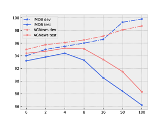
Figure 2: Performances on dev and test sets w.r.t. the number of generated training examples for each misclassified test example.

Since we don’t have access to the test set, we use the dev set to perturb training examples. For each erroneously classified example in the dev set, we generate perturbed training examples, trying to flip the decision. Instead of replacing training examples, perturbations are additionally added to the training set. With the combined training set, a model is retrained and we report test performances. Results are shown in Figure 2. As we can see, the trends for both IMDB and AG News are the same: when we gradually increase the number of training examples generated for each misclassified test example from 0 to 8, the test performance increases accordingly. But as we continue increasing training examples, the model trained on the generated training examples starts overfitting the dev set, leading to drastic drops in test performances. We obtain the best test results at # Examples = 4, giving a +1 accuracy gain compared to models without augmentation.

5 Conclusion

In this paper, we propose a paradigm that unifies test-focused methods and training-focuses for interpreting a neural network model’s prediction. The proposed paradigm answers the question of because of which part(s) of which training example(s), the model attends to which part(s) of a given test example. We demonstrate that the proposed methodology offers clear explanations about neural model decisions, along with being useful for error analysis and creating adversarial examples.

Appendix A Derivation of The Influence Function

In this section, we follow Koh and Liang (2017) to prove the following expression (Eq.4):

$$I(z,{\theta})\triangleq\frac{\mathrm{d}{\theta}_{z,\epsilon}}{\mathrm{d}\epsilon}\Big{|}_{\epsilon=0}=-H^{-1}_{{\theta}}\nabla_{\theta}L(z;{\theta})$$ (13)

Recall that ${\theta}$ minimizes the empirical risk $R(\theta)$:

$$R(\theta)\triangleq\frac{1}{n}\sum_{i=1}^{n}L(z_{i};\theta)$$ (14)

and $\theta_{z,\epsilon}$ minimizes the following upweighted empirical risk:

$$R(\theta)+\epsilon L(z;\theta)$$ (15)

Therefore, we have the following identities hold:

$$\nabla R(\theta) =0$$ (16)

$$\nabla R(\theta_{z,\epsilon})+\nabla\epsilon L(z;\theta_{z,\epsilon}) =0$$

for which we can apply first-order Taylor expansion to the second expression:

$$0\approx \left[\nabla R({\theta})+\epsilon\nabla L(z;{\theta})\right]$$ (17)

$$\left[\nabla^{2}R({\theta})+\epsilon\nabla^{2}L(z;{\theta})\right]\Delta_{\epsilon}$$

where $\Delta_{\epsilon}={\theta}_{z,\epsilon}-{\theta}$ is the parameter change. Solving for $\Delta_{\epsilon}$, we have:

$$\Delta_{\epsilon}\approx -\left[\nabla^{2}R({\theta})+\epsilon\nabla^{2}L(z;{\theta})\right]^{-1}$$ (18)

$$\left[\nabla R({\theta})+\epsilon\nabla L(z;{\theta})\right]$$

Dropping higher order terms of $\epsilon$ and plugging $\nabla R(\theta)=0$ in, we have:

$$\Delta_{\epsilon}\approx-\nabla^{2}R({\theta})^{-1}\nabla L(z;{\theta})\epsilon$$ (19)

which shows that

$$\frac{\mathrm{d}{\theta}_{z,\epsilon}}{\mathrm{d}\epsilon}=\frac{\mathrm{d}\Delta_{\epsilon}}{\mathrm{d}\epsilon}\Big{|}_{\epsilon=0}=-H^{-1}_{{\theta}}\nabla_{\theta}L(z;{\theta})$$ (20)

Appendix B Efficient Computation of The Hessian

Albeit its appealing properties for approximating influences, calculating the full Hessian $H_{{\theta}}$ is too expensive to afford. To efficiently calculate it, we follow Koh and Liang (2017) to use the method of stochastic estimation proposed by Agarwal et al. (2016) and the Hessian-Vector Product (HVP) trick (Pearlmutter, 1994) to get an estimator that only samples a single point per iteration, leading to a trade-off between speed and accuracy.

Concretely, we let $H^{-1}_{j}\triangleq\sum_{i=0}^{j}(I-H)^{i}$ be the first $j$ terms in the matrix Taylor expansion of $H^{-1}$, which can be recursively written as $H_{j}^{-1}=I+(I-H)H^{-1}_{j-1}$. It can be validated that $H^{-1}_{j}\to H^{-1}$ as $j\to\infty$. So we can replace $H$ with a single drawn point from the training set, and iteratively recover $H^{-1}$.

In particular, we first uniformly sample $t$ points $z_{s_{1}},\cdots,z_{s_{t}}$ from the training data, and define $\tilde{H}_{0}^{-1}v=v$. Then we recursively compute $\tilde{H}_{j}^{-1}v=v+(I-\nabla_{\theta}^{2}L(z_{s_{j}};{\theta}))\tilde{H}^{-1}_{j-1}v$ according to the above expression. After $t$ iterations, we take $\tilde{H}^{-1}_{t}v$ as the final unbiased estimate of $H^{-1}v$. We pick $t$ such that $\tilde{H}_{t}$ stabilizes. To further reduce variance we repeat this process $r$ times and average the results. Afterwards, we apply the process to calculate the Hessian-vector products in $I(z,\theta),I(z,w_{y}(\mathbf{e}))$ and $I(z,\tilde{z},\theta),I(z,\tilde{z},w_{y}(\mathbf{e}))$.

References

- Adler et al. (2018) Philip Adler, Casey Falk, Sorelle A Friedler, Tionney Nix, Gabriel Rybeck, Carlos Scheidegger, Brandon Smith, and Suresh Venkatasubramanian. 2018. Auditing black-box models for indirect influence. Knowledge and Information Systems, 54(1):95–122.
- Agarwal et al. (2016) Naman Agarwal, Brian Bullins, and Elad Hazan. 2016. Second-order stochastic optimization in linear time. stat, 1050:15.
- Alvarez-Melis and Jaakkola (2017) David Alvarez-Melis and Tommi S Jaakkola. 2017. A causal framework for explaining the predictions of black-box sequence-to-sequence models. arXiv preprint arXiv:1707.01943.
- Alzantot et al. (2018) Moustafa Alzantot, Yash Sharma, Ahmed Elgohary, Bo-Jhang Ho, Mani Srivastava, and Kai-Wei Chang. 2018. Generating natural language adversarial examples. arXiv preprint arXiv:1804.07998.
- Athalye et al. (2018) Anish Athalye, Logan Engstrom, Andrew Ilyas, and Kevin Kwok. 2018. Synthesizing robust adversarial examples. In International conference on machine learning, pages 284–293. PMLR.
- Bach et al. (2015a) Sebastian Bach, Alexander Binder, Grégoire Montavon, Frederick Klauschen, Klaus-Robert Müller, and Wojciech Samek. 2015a. On pixel-wise explanations for non-linear classifier decisions by layer-wise relevance propagation. PloS one, 10(7).
- Bach et al. (2015b) Sebastian Bach, Alexander Binder, Grégoire Montavon, Frederick Klauschen, Klaus-Robert Müller, and Wojciech Samek. 2015b. On pixel-wise explanations for non-linear classifier decisions by layer-wise relevance propagation. PLOS ONE, 10:1–46.
- Barham and Feizi (2019) Samuel Barham and Soheil Feizi. 2019. Interpretable adversarial training for text. arXiv preprint arXiv:1905.12864.
- Biggio et al. (2012) Battista Biggio, Blaine Nelson, and Pavel Laskov. 2012. Poisoning attacks against support vector machines. arXiv preprint arXiv:1206.6389.
- Clark et al. (2019) Kevin Clark, Urvashi Khandelwal, Omer Levy, and Christopher D. Manning. 2019. What does bert look at? an analysis of bert’s attention.
- Cook (1986) R Dennis Cook. 1986. Assessment of local influence. Journal of the Royal Statistical Society: Series B (Methodological), 48(2):133–155.
- Cook and Weisberg (1982) R Dennis Cook and Sanford Weisberg. 1982. Residuals and influence in regression. New York: Chapman and Hall.
- Datta et al. (2016) Anupam Datta, Shayak Sen, and Yair Zick. 2016. Algorithmic transparency via quantitative input influence: Theory and experiments with learning systems. In 2016 IEEE symposium on security and privacy (SP), pages 598–617. IEEE.
- Devlin et al. (2018) Jacob Devlin, Ming-Wei Chang, Kenton Lee, and Kristina Toutanova. 2018. Bert: Pre-training of deep bidirectional transformers for language understanding. arXiv preprint arXiv:1810.04805.
- Ebrahimi et al. (2017) Javid Ebrahimi, Anyi Rao, Daniel Lowd, and Dejing Dou. 2017. Hotflip: White-box adversarial examples for text classification. arXiv preprint arXiv:1712.06751.
- Ghaeini et al. (2018) Reza Ghaeini, Xiaoli Z Fern, and Prasad Tadepalli. 2018. Interpreting recurrent and attention-based neural models: a case study on natural language inference. arXiv preprint arXiv:1808.03894.
- Glorot et al. (2011) Xavier Glorot, Antoine Bordes, and Yoshua Bengio. 2011. Deep sparse rectifier neural networks. In Proceedings of the fourteenth international conference on artificial intelligence and statistics, pages 315–323.
- Goodfellow et al. (2014) Ian J Goodfellow, Jonathon Shlens, and Christian Szegedy. 2014. Explaining and harnessing adversarial examples. arXiv preprint arXiv:1412.6572.
- Greff et al. (2016) Klaus Greff, Rupesh K Srivastava, Jan Koutník, Bas R Steunebrink, and Jürgen Schmidhuber. 2016. Lstm: A search space odyssey. IEEE transactions on neural networks and learning systems, 28(10):2222–2232.
- Han et al. (2020) Xiaochuang Han, Byron C Wallace, and Yulia Tsvetkov. 2020. Explaining black box predictions and unveiling data artifacts through influence functions. arXiv preprint arXiv:2005.06676.
- He et al. (2016) Kaiming He, Xiangyu Zhang, Shaoqing Ren, and Jian Sun. 2016. Deep residual learning for image recognition. In Proceedings of the IEEE conference on computer vision and pattern recognition, pages 770–778.
- Hermans and Schrauwen (2013) Michiel Hermans and Benjamin Schrauwen. 2013. Training and analysing deep recurrent neural networks. In Advances in neural information processing systems, pages 190–198.
- Jain and Wallace (2019) Sarthak Jain and Byron C. Wallace. 2019. Attention is not explanation.
- Jia et al. (2019) Robin Jia, Aditi Raghunathan, Kerem Göksel, and Percy Liang. 2019. Certified robustness to adversarial word substitutions. arXiv preprint arXiv:1909.00986.
- Kádár et al. (2017) Akos Kádár, Grzegorz Chrupała, and Afra Alishahi. 2017. Representation of linguistic form and function in recurrent neural networks. Computational Linguistics, 43(4):761–780.
- Karpathy et al. (2015) Andrej Karpathy, Justin Johnson, and Li Fei-Fei. 2015. Visualizing and understanding recurrent networks. arXiv preprint arXiv:1506.02078.
- Kindermans et al. (2017) Pieter-Jan Kindermans, Kristof T. Schütt, Maximilian Alber, Klaus-Robert Müller, Dumitru Erhan, Been Kim, and Sven Dähne. 2017. Learning how to explain neural networks: Patternnet and patternattribution.
- Koh and Liang (2017) Pang Wei Koh and Percy Liang. 2017. Understanding black-box predictions via influence functions. In Proceedings of the 34th International Conference on Machine Learning-Volume 70, pages 1885–1894. JMLR. org.
- Kurakin et al. (2016) Alexey Kurakin, Ian Goodfellow, and Samy Bengio. 2016. Adversarial examples in the physical world. arXiv preprint arXiv:1607.02533.
- Lei et al. (2016) Tao Lei, Regina Barzilay, and Tommi Jaakkola. 2016. Rationalizing neural predictions. arXiv preprint arXiv:1606.04155.
- Li et al. (2015a) Jiwei Li, Xinlei Chen, Eduard Hovy, and Dan Jurafsky. 2015a. Visualizing and understanding neural models in nlp. arXiv preprint arXiv:1506.01066.
- Li et al. (2015b) Jiwei Li, Thang Luong, Dan Jurafsky, and Eduard Hovy. 2015b. When are tree structures necessary for deep learning of representations? In Proceedings of the 2015 Conference on Empirical Methods in Natural Language Processing, pages 2304–2314, Lisbon, Portugal. Association for Computational Linguistics.
- Li et al. (2016) Jiwei Li, Will Monroe, and Dan Jurafsky. 2016. Understanding neural networks through representation erasure. arXiv preprint arXiv:1612.08220.
- Lundberg and Lee (2017) Scott M Lundberg and Su-In Lee. 2017. A unified approach to interpreting model predictions. In Advances in neural information processing systems, pages 4765–4774.
- Maas et al. (2011) Andrew L Maas, Raymond E Daly, Peter T Pham, Dan Huang, Andrew Y Ng, and Christopher Potts. 2011. Learning word vectors for sentiment analysis. In Proceedings of the 49th annual meeting of the association for computational linguistics: Human language technologies-volume 1, pages 142–150. Association for Computational Linguistics.
- Madry et al. (2017) Aleksander Madry, Aleksandar Makelov, Ludwig Schmidt, Dimitris Tsipras, and Adrian Vladu. 2017. Towards deep learning models resistant to adversarial attacks. arXiv preprint arXiv:1706.06083.
- Mei and Zhu (2015) Shike Mei and Xiaojin Zhu. 2015. Using machine teaching to identify optimal training-set attacks on machine learners. In AAAI, pages 2871–2877.
- Miyato et al. (2016) Takeru Miyato, Andrew M. Dai, and Ian Goodfellow. 2016. Adversarial training methods for semi-supervised text classification.
- Montavon et al. (2017) Grégoire Montavon, Sebastian Lapuschkin, Alexander Binder, Wojciech Samek, and Klaus-Robert Müller. 2017. Explaining nonlinear classification decisions with deep taylor decomposition. Pattern Recognition, 65:211–222.
- Moosavi-Dezfooli et al. (2016) Seyed-Mohsen Moosavi-Dezfooli, Alhussein Fawzi, and Pascal Frossard. 2016. Deepfool: a simple and accurate method to fool deep neural networks. In Proceedings of the IEEE conference on computer vision and pattern recognition, pages 2574–2582.
- Muñoz-González et al. (2017) Luis Muñoz-González, Battista Biggio, Ambra Demontis, Andrea Paudice, Vasin Wongrassamee, Emil C Lupu, and Fabio Roli. 2017. Towards poisoning of deep learning algorithms with back-gradient optimization. In Proceedings of the 10th ACM Workshop on Artificial Intelligence and Security, pages 27–38.
- Papernot et al. (2017) Nicolas Papernot, Patrick McDaniel, Ian Goodfellow, Somesh Jha, Z Berkay Celik, and Ananthram Swami. 2017. Practical black-box attacks against machine learning. In Proceedings of the 2017 ACM on Asia conference on computer and communications security, pages 506–519.
- Papernot et al. (2016) Nicolas Papernot, Patrick McDaniel, Ananthram Swami, and Richard Harang. 2016. Crafting adversarial input sequences for recurrent neural networks. In MILCOM 2016-2016 IEEE Military Communications Conference, pages 49–54. IEEE.
- Pearlmutter (1994) Barak A. Pearlmutter. 1994. Fast exact multiplication by the hessian. Neural Comput., 6(1):147–160.
- Ren et al. (2019) Shuhuai Ren, Yihe Deng, Kun He, and Wanxiang Che. 2019. Generating natural language adversarial examples through probability weighted word saliency. In Proceedings of the 57th annual meeting of the association for computational linguistics, pages 1085–1097.
- Ribeiro et al. (2016) Marco Tulio Ribeiro, Sameer Singh, and Carlos Guestrin. 2016. ”why should i trust you?”: Explaining the predictions of any classifier.
- Sato et al. (2018) Motoki Sato, Jun Suzuki, Hiroyuki Shindo, and Yuji Matsumoto. 2018. Interpretable adversarial perturbation in input embedding space for text. In Proceedings of the Twenty-Seventh International Joint Conference on Artificial Intelligence, IJCAI-18, pages 4323–4330. International Joint Conferences on Artificial Intelligence Organization.
- Schwab and Karlen (2019) Patrick Schwab and Walter Karlen. 2019. Cxplain: Causal explanations for model interpretation under uncertainty. In Advances in Neural Information Processing Systems, pages 10220–10230.
- Serrano and Smith (2019) Sofia Serrano and Noah A Smith. 2019. Is attention interpretable? arXiv preprint arXiv:1906.03731.
- Shafahi et al. (2018) Ali Shafahi, W. Ronny Huang, Mahyar Najibi, Octavian Suciu, Christoph Studer, Tudor Dumitras, and Tom Goldstein. 2018. Poison frogs! targeted clean-label poisoning attacks on neural networks. In S. Bengio, H. Wallach, H. Larochelle, K. Grauman, N. Cesa-Bianchi, and R. Garnett, editors, Advances in Neural Information Processing Systems 31, pages 6103–6113. Curran Associates, Inc.
- Shi et al. (2016) Xing Shi, Kevin Knight, and Deniz Yuret. 2016. Why neural translations are the right length. In Proceedings of the 2016 Conference on Empirical Methods in Natural Language Processing, pages 2278–2282, Austin, Texas. Association for Computational Linguistics.
- Shrikumar et al. (2017) Avanti Shrikumar, Peyton Greenside, and Anshul Kundaje. 2017. Learning important features through propagating activation differences. arXiv preprint arXiv:1704.02685.
- Simonyan et al. (2013) Karen Simonyan, Andrea Vedaldi, and Andrew Zisserman. 2013. Deep inside convolutional networks: Visualising image classification models and saliency maps. arXiv preprint arXiv:1312.6034.
- Socher et al. (2013) Richard Socher, Alex Perelygin, Jean Wu, Jason Chuang, Christopher D Manning, Andrew Y Ng, and Christopher Potts. 2013. Recursive deep models for semantic compositionality over a sentiment treebank. In Proceedings of the 2013 conference on empirical methods in natural language processing, pages 1631–1642.
- Springenberg et al. (2014) Jost Tobias Springenberg, Alexey Dosovitskiy, Thomas Brox, and Martin Riedmiller. 2014. Striving for simplicity: The all convolutional net. arXiv preprint arXiv:1412.6806.
- Srinivas and Fleuret (2019) Suraj Srinivas and François Fleuret. 2019. Full-gradient representation for neural network visualization. In Advances in Neural Information Processing Systems, pages 4124–4133.
- Strobelt et al. (2016) Hendrik Strobelt, Sebastian Gehrmann, Bernd Huber, Hanspeter Pfister, Alexander M Rush, et al. 2016. Visual analysis of hidden state dynamics in recurrent neural networks. arXiv preprint arXiv:1606.07461.
- Sundararajan et al. (2017) Mukund Sundararajan, Ankur Taly, and Qiqi Yan. 2017. Axiomatic attribution for deep networks. arXiv preprint arXiv:1703.01365.
- Tai et al. (2015) Kai Sheng Tai, Richard Socher, and Christopher D Manning. 2015. Improved semantic representations from tree-structured long short-term memory networks. arXiv preprint arXiv:1503.00075.
- Tenney et al. (2019) Ian Tenney, Dipanjan Das, and Ellie Pavlick. 2019. Bert rediscovers the classical nlp pipeline. arXiv preprint arXiv:1905.05950.
- Vashishth et al. (2019) Shikhar Vashishth, Shyam Upadhyay, Gaurav Singh Tomar, and Manaal Faruqui. 2019. Attention interpretability across nlp tasks. arXiv preprint arXiv:1909.11218.
- Vaswani et al. (2017) Ashish Vaswani, Noam Shazeer, Niki Parmar, Jakob Uszkoreit, Llion Jones, Aidan N Gomez, Ł ukasz Kaiser, and Illia Polosukhin. 2017. Attention is all you need. In I. Guyon, U. V. Luxburg, S. Bengio, H. Wallach, R. Fergus, S. Vishwanathan, and R. Garnett, editors, Advances in Neural Information Processing Systems 30, pages 5998–6008. Curran Associates, Inc.
- Vig and Belinkov (2019) Jesse Vig and Yonatan Belinkov. 2019. Analyzing the structure of attention in a transformer language model. arXiv preprint arXiv:1906.04284.
- Wallace et al. (2019) Eric Wallace, Jens Tuyls, Junlin Wang, Sanjay Subramanian, Matt Gardner, and Sameer Singh. 2019. Allennlp interpret: A framework for explaining predictions of nlp models. arXiv preprint arXiv:1909.09251.
- Wang et al. (2020) Xiaosen Wang, Yichen Yang, Yihe Deng, and Kun He. 2020. Fast gradient projection method for text adversary generation and adversarial training. arXiv preprint arXiv:2008.03709.
- Wiegreffe and Pinter (2019) Sarah Wiegreffe and Yuval Pinter. 2019. Attention is not not explanation. In Proceedings of the 2019 Conference on Empirical Methods in Natural Language Processing and the 9th International Joint Conference on Natural Language Processing (EMNLP-IJCNLP), pages 11–20, Hong Kong, China. Association for Computational Linguistics.
- Zeiler and Fergus (2014) Matthew D Zeiler and Rob Fergus. 2014. Visualizing and understanding convolutional networks. In European conference on computer vision, pages 818–833. Springer.
- Zhang et al. (2020) Huangzhao Zhang, Zhuo Li, Ge Li, Lei Ma, Yang Liu, and Zhi Jin. 2020. Generating adversarial examples for holding robustness of source code processing models. 34:1169–1176.
- Zhang et al. (2018) Quanshi Zhang, Yu Yang, Yuchen Liu, Ying Nian Wu, and Song-Chun Zhu. 2018. Unsupervised learning of neural networks to explain neural networks. arXiv preprint arXiv:1805.07468.
- Zhao et al. (2017) Zhengli Zhao, Dheeru Dua, and Sameer Singh. 2017. Generating natural adversarial examples. arXiv preprint arXiv:1710.11342.
- Zhou et al. (2020) Yi Zhou, Xiaoqing Zheng, Cho-Jui Hsieh, Kai-wei Chang, and Xuanjing Huang. 2020. Defense against adversarial attacks in nlp via dirichlet neighborhood ensemble. arXiv preprint arXiv:2006.11627.
- Zhu et al. (2020) Chen Zhu, Yu Cheng, Zhe Gan, Siqi Sun, Tom Goldstein, and Jingjing Liu. 2020. Freelb: Enhanced adversarial training for natural language understanding. In International Conference on Learning Representations.