PP-LinkNet: Improving Semantic Segmentation of High Resolution Satellite Imagery with Multi-stage Training

Abstract.

Road network and building footprint extraction is essential for many applications such as updating maps, traffic regulations, city planning, ride-hailing, disaster response etc. Mapping road networks is currently both expensive and labor-intensive. Recently, improvements in image segmentation through the application of deep neural networks has shown promising results in extracting road segments from large scale, high resolution satellite imagery. However, significant challenges remain due to lack of enough labeled training data needed to build models for industry grade applications. In this paper, we propose a two-stage transfer learning technique to improve robustness of semantic segmentation for satellite images that leverages noisy pseudo ground truth masks obtained automatically (without human labor) from crowd-sourced OpenStreetMap (OSM) data. We further propose Pyramid Pooling-LinkNet (PP-LinkNet), an improved deep neural network for segmentation that uses focal loss, poly learning rate, and context module. We demonstrate the strengths of our approach through evaluations done on three popular datasets over two tasks, namely, road extraction and building foot-print detection. Specifically, we obtain 78.19% meanIoU on SpaceNet building footprint dataset, 67.03% and 77.11% on the road topology metric on SpaceNet and DeepGlobe road extraction dataset, respectively.

1. Introduction

Maps are common heritage for humanity. Creating and updating maps is an important task with many potential applications in disaster recovery, geospatial search, urban planning, ride-hailing industry, etc (Demir et al., 2018a). Today, map features such as roads, building footprints, and points of interest are primarily created through manual techniques. We address the problem of extracting road networks and building footprints automatically from satellite imagery in this paper.

Maps of roads and buildings are expensive to build and maintain. Although modern cartography involves using satellite and aerial imagery along with GPS traces, using these data to update maps involves having humans analyze the data in a time consuming process, and thus maps of rapidly growing cities (where infrastructure is constantly under construction) are still often inaccurate and incomplete outside the urban core. Current approaches to map inference via satellite images (Van Etten et al., 2018; Demir et al., 2018b) involve extensive annotations of images that is both tedious and time consuming.

Currently, we have two large public datasets containing satellite images of road networks with annotations: i) SpaceNet (Van Etten et al., 2018) and DeepGlobe (Demir et al., 2018b). SpaceNet challenge 3 road extraction (Van Etten et al., 2018) only provides 2779 training satellite images of Las Vegas, Paris, Shanghai, Khartoum with image size of $1300\times 1300$ with their road center-line annotations. ii) DeepGlobe (Demir et al., 2018b) has a total of 8570 images with 6226 training, 1243 validation and 1101 testing images with pixel-based annotations, where all pixels belonging to the road are labeled, instead of labeling only center-line. Although seemingly large, these datasets are still not enough to train a robust model for analyzing satellite imagery on a global scale due to challenges posed by spatial variations – roads differ in their appearance due to regional terrain, urban vs rural divide, state of economy, e.g., developed vs. developing countries, see Figure 2) and temporal variations resulting in images captured during different seasons with varying lighting conditions, cloud cover, etc. In this paper, we develop an efficient and effective technique to fine-tune semantic segmentation models robustly on different variances of satellite images. The centered idea is that we leverage OpenStreetMap(OSM) data to generate noisy pseudo ground truth of road network or building footprint and utilize it in the training process.

Our contributions are three-fold. First, we develop a novel method to generate pseudo road network and building footprint ground truth masks from OSM data without human annotation labor. Second, we propose a two-stage transfer learning to utilize the pseudo ground truth masks in the first stage, and fine-tune the model on high quality annotation data in the second stage. In addition, we also propose some techniques and architectural modifications, i.e., PP-LinkNet, to improve the overall performance of the binary semantic segmentation system to extract road networks and building footprints from satellite images. Finally, we achieve promising improvements on DeepGlobe road network dataset(Demir et al., 2018b), SpaceNet road and building footprint dataset (Van Etten et al., 2018).

Figure 1. Illustration of the rasterization process to convert OpenStreetMap data into pseudo ground truth mask image. Top row: rasterization using TileMill software. Bottom row: our rasterization using OpenCV from the corresponding road network graph. Best viewed in color.

2. Related Work

Datasets for road network. Two large datasets for road network extraction from satellite imagery (i.e., SpaceNet (Van Etten et al., 2018) and DeepGlobe (Demir et al., 2018b)). They differ mainly in the format of annotation data – while SpaceNet dataset provides centerlines for roads, DeepGlobe provides pixel labeling of roads. Several published works use proprietary datasets that are not available in the public domain for bench marking, e.g., (Mattyus et al., 2015, 2017; Wang et al., 2017; Bastani et al., 2018).

Semantic segmentation models for road network extraction. Inspired by successes of deep learning in computer vision (He et al., 2016; Ren et al., 2015; He et al., 2017; Luo et al., 2015; Tran and Cheong, 2017), there have been few attempts in addressing the problem of road extraction from satellite images using deep learning based semantic segmentation models. D-LinkNet (Zhou et al., 2018), the winner model of DeepGlobe road extraction challenge, utilizes LinkNet(Chaurasia and Culurciello, 2017), UNet(Ronneberger et al., 2015), ResNet (He et al., 2016) and dilated convolution(Chen et al., 2018) components model and improvises using a post-processing step to refine the segmentation output to a road network graph. DeepRoadMapper (Mattyus et al., 2017) developed a model based on ResNet (He et al., 2016) and FCN (Shelhamer et al., 2015), and a technique to infer missing connections from segmentation results. On the other hand, RoadTracer (Bastani et al., 2018) uses convolutional neural network (CNN) to predict the walking angle of the sliding window on the input image to decide on the input image for the next iteration.

Our work is similar to (Audebert et al., 2017), where the authors use OSM data along with satellite imagery to predict semantic map features (e.g., surfaces, buildings, vegetables, trees, cars, etc). On the contrary, our work utilizes OSM as pseudo ground truth data only in the first stage of our two-stage transfer learning.

3. Generating noisy pseudo ground truth

In this section, we describe our approach to collect a large-scale satellite image dataset along with its pseudo ground truth to train road network and building footprint segmentation model in the first stage.

3.1. Rasterization of OSM data into pseudo (noisy) ground truth image

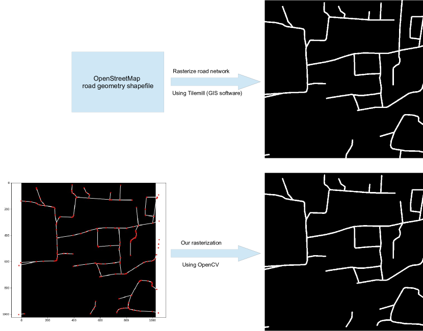
In order to avoid laborious annotation work and to create a scalable approach towards creating training data we relied on OpenStreetMap (OSM)(Humanitarian OpenStreetMap Team, [n.d.]), a large community driven map. OSM data contains many useful metadata information such as type of roads, number of lanes, width, surface, bridge, tunnel, etc. Our source of satellite imagery is from different sources of remotely sensed data. The procedure to extract ground truth from OSM data is as follows: i) collect satellite images for the area of interest, i) render the road-network from OSM using TileMill software. This rendering process is called the rasterization process in the geographical information system (GIS) community. There are few GIS softwares that can do rasterization such as TileMill, QGIS, ArcGIS, etc. Furthermore, we also develop our rasterization process using OpenCV. Specifically, our process is to draw lines with certain widths corresponding to locations of roads in the image. Figure 1 shows that our rasterization process would produce similar pseudo ground truth image with the result from TileMill software. We use our rasterization process using OpenCV through all our experiments. Our rasterization process is based on the transformation matrix $\mathcal{T}$ available in tif-format satellite image, as in equation 1),

(1) $$(lon,lat)=\mathcal{T}*(r+0.5,c+0.5,1),$$

where $(lon,lat)$ is the longitude, latitude according to the image coordinate $(c,r)$. From equation 1, given the longitude, latitude of a node in OSM road networks, we can infer its image coordinates from the inverse matrix of the transformation matrix $\mathcal{T}$.

There are three main advantages of our approach of using noisy pseudo ground truth images as part of training data. First, annotating pixel-to-pixel for large image size of satellite images (e.g., $1024\times 1024$) is an exhaustive task. Generating ground truth through rasterizing OSM data is efficient so that we can scale the number of training images up easily. Second, the pseudo ground truth of satellite imagery is generally available for most locations on earth. We only need to know the geographical address of the locations to rasterize the pseudo ground truth masks. Finally, the accuracy of OSM ground truth is enough to train a moderate model in the first phase. Hence, we devised a second phase in order to fine-tune our model with high quality annotated ground truth.

Figure 2. Columns represent examples of inputs: satellite imagery, pseudo ground truth mask, and overlay of ground truth mask on input image. First row: a satellite image of Jakarta; second row: a input image of Las Vegas city in SpaceNet dataset.

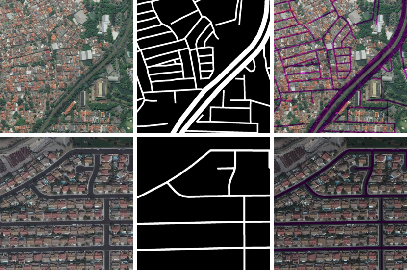
Figure 2 shows an example of a pair of input and its rasterized pseudo ground truth mask in Las Vegas city from SpaceNet dataset. Although the structure of road network in the example is correct with the satellite image, its pixel-to-pixel matching is limited. Sometimes, the pseudo ground truth is smaller or bigger than the actual road, hence, it is called pseudo ground truth.

3.2. Image collection

We build our training data in the first stage by combining data from SpaceNet (Van Etten et al., 2018), DeepGlobe (Demir et al., 2018b), and our internal data. Both SpaceNet and DeepGlobe datasets have high resolution satellite images (i.e., 0.3-0.5m). We remove some imperfect images of SpaceNet (Van Etten et al., 2018), which has zero signal due to sensor’s errors. The DeepGlobe (Demir et al., 2018b) images are sampled from DigitalGlobe Vivid imagery which contains cloud-free, high resolution satellite images. Furthermore, we also collect our own data from additional sources such as internal data, EarthExplorer (USGS, [n.d.]), etc. Currently, our dataset has two resolutions $1024\times 1024$ and $1300\times 1300$. We decide to build the dataset with high resolution satellite images because we consider the narrowness, connectivity, complexity, and long span of roads. Eventually, we utilize 48091 images and their corresponding noisy pseudo ground truth masks to train the model of road network segmentation in the first phase.

4. Method

We formulate our task of extracting roads from satellite images as a binary semantic image segmentation problem, where for each input satellite image, we predict if a pixel belongs to class 1 (Road) or class 0 (non-road). Distinct from datasets for object detection such as PASCAL VOC 2012 (Neuhold et al., 2017) and MS-COCO (Lin et al., 2014), satellite images need to be processed at a high resolution (e.g., $1024\times 1024$). This compels the need to design our network with efficient memory optimisations.

4.1. Network Architecture Design

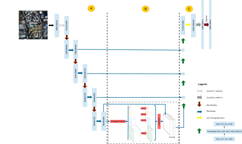
Figure 3 shows an overview of our proposed network architecture Pyramid Pooling-LinkNet (PP-LinkNet). Our network design is inspired by the encoder-decoder architecture such as Unet (Ronneberger et al., 2015). We received input images at resolutions of $1024\times 1024$, hence, we emphasize on efficient network structure. We choose LinkNet (Chaurasia and Culurciello, 2017) as our base network, similar to D-LinkNet (Zhou et al., 2018). Our encoder is ResNet34 (He et al., 2016) pre-trained on ImageNet dataset. RestNet34 is originally trained to classify images of mid-resolution $256\times 256$, whereas, our task is to segment roads and building footprints from higher resolution imagery $1024\times 1024$. Therefore, the network needs to adapt encoder layers to new domain of input. Our decoder includes bottleneck blocks, and layers of decoder up-sample feature size to have symmetric sizes with encoder’s layers. The bottleneck block of a decoder consists of a transposed convolutional layer between two convolutional layers with $(1\times 1)$-kernels (see Figure 3). Our decoder is initialized with random parameters. In the middle of our network is global contextual prior, pyramid pooling (PP) module, which has been empirically proven to be effective in PSPNet (Zhao et al., 2017). Pyramid pooling module has no parameters, and proven to have better performance than the context module in D-LinkNet in our experiments.

Figure 3. Overview of our proposed network architecture PP-LinkNet. It is an improvement of D-LinkNet(Zhou et al., 2018) with the replacement of enlarged receptive field module with pyramid pooling module in PSPNet (Zhao et al., 2017). Each blue block is a multi-dimensional feature which is an output from a block of convolutional layers (except the last layer is a sigmoid layer). Part A: encoder; part B: pyramid pooling module, part C: decoder. Best viewed in color.

4.2. Improvements of semantic segmentation system for road network extraction

Two-stage transfer learning. In the first phase, we train our PP-LinkNet on noisy pseudo ground truth generated from OSM (Sect. 3) to let the network learn basic visual features and knowledge of the new domain (i.e., aerial or satellite imagery). For the second phase, we propose a simple transfer learning procedure to fine-tune the trained model one more time with high-quality well-annotated data.

Class imbalance. It is obvious that the number of non-road pixels is much bigger than the number of road pixels. This extreme class imbalance causes our network to pay more attention to background pixels to learn weights of semantic segmentation systems. Focal loss has been proposed in (Lin et al., 2017) to tackle class imbalanced foreground and background sampled bounding boxes in object detection pipelines. Focal loss for each pixel $FL(p_{i,t})$ and for an image $FL$ can be expressed as

(2) $$FL(p_{i,t})=-\alpha_{t}(1-p_{i,t})^{\gamma}\log(p_{i,t})$$

$$FL=\sum_{i}^{N}FL(p_{i,t}),$$

where $p_{i,t}$ is the model’s estimated probability for the class with label $y=t$. Specifically, we have two class, non-road and road, $\{0,1\}$ and $p\in[0,1]$ is the estimated probability for the class with label $y=1$, then

(3) $$p_{t}=\begin{cases}p,&\mbox{if y=1}\\ 1-p,&\mbox{otherwise.}\end{cases}$$

From different experiments, we found that $-\alpha_{t},\gamma=0.5$ is the best parameters for the focal loss function $FL(p_{i,t})$.

Proposed in (Milletari et al., 2016), Dice coefficient loss, denoted as $DL$, can be written as

(4) $$DL=1-\dfrac{2\sum_{i}^{N}p_{i}g_{i}+\epsilon}{\sum_{i}^{N}p_{i}^{2}+\sum_{i}^{N}g_{i}^{2}+\epsilon},$$

where $N$ is the number of pixels in image, $p_{i}\in[0,1]$ is the predicted probability of a pixel, and $g_{i}\in\{0,1\}$ is the binary ground truth of the pixel. The $\epsilon$ term is a small constant to ensure the loss function stability by preventing numerical issues of dividing by 0. The Dice loss originated from Sørensen–Dice coefficient (Dic, [n.d.]), a statistic used for comparing similarity between two samples. Optimally, when we minimize $DL$ loss, an optimizer would increase $p_{i}$ for foreground pixels (i.e., $g_{i}=1$) and decrease $p_{i}$ for background pixels (i.e., $g_{i}=1$). Dice loss does not suffer from class imbalance because contributions of individual pixels only influence numerator or denominator term, not the whole loss function.

Poly learning rate policy. Similar to (Chen et al., 2018; Liu et al., 2016), we also explore a “poly” learning rate policy (i.e., the learning rate is equal to the base learning rate multiplied by $(1-\dfrac{iter}{max\_iter})^{power}$) with $power=0.9$ for training DLinkNet.

Context module. One improvement of PP-LinkNet compared to D-LinkNet is the pyramid pooling context module. We integrate the pyramid pooling module (Zhao et al., 2017) into LinkNet (Chaurasia and Culurciello, 2017) between encoder and decoder part. Through our empirical experiments, we found that the pyramid pooling module with no parameters is effective in improving performance of our model, hence, we named it PP-LinkNet (i.e., PyramidPooling-LinkNet).

(a) Three loss functions

(b) Effects of poly learning rate

Figure 4. $\left(a\right)$. Training loss of three different loss functions: focal loss, dice loss, binary cross entropy loss. $\left(b\right)$ Comparison of training losses between reduce-on-plateau and poly learning rate policy. The experiments are done with the same settings: data, batch size, learning rate. The loss values are averaged per epoch.

5. Experiments

5.1. Dataset

DeepGlobe road extraction (Demir et al., 2018b). Road extraction task in DeepGlobe challenge has 6226 training, 1243 validation, and 1101 testing images, with image resolution of $1024\times 1024$. The ground resolution is 50 cm/pixel. However, we don’t have annotations for validation and testing images. We follow (Singh et al., 2018) to split the training image set into 4696 images for training and 1530 for validation.

SpaceNet challenge 2 building footprints (Demir et al., 2018b). The dataset includes 24,586 images of size $650\times 650$ containing 302,701 building footprints across Las Vegas, Paris, Shanghai, Khartoum. The ground resolution is 30 cm/pixel. We split the training set of dataset into 80%/20% for training/test, equivalently to, 8472 images for training and 2121 for testing. We conduct experiments on only 3 RGB channels of multi-spectral images, and on full resolution $650\times 650$ of input images. More information about F1 evaluation metric of the dataset can be found in DeepGlobe building detection task (Demir et al., 2018b).

SpaceNet challenge 3 road extraction (Demir et al., 2018b). The dataset includes 2780 images, and, following (Singh et al., 2018), we split the dataset into 2213 images for training and 567 images for testing. The ground truth is represented by line strings, indicating center-lines of the roads. The image has a resolution of $1300\times 1300$, and its ground resolution is 30cm/pixel. Unlike (Batra et al., 2019), we train our model on larger image crop $1024\times 1024$, not $512\times 512$. As human errors, we always have some mistakes in annotations of three datasets, but we leave it for future analyses.

5.2. Goal and Metrics

Pixel based metric. The semantic segmentation algorithm is expected to predict a mask for a test image (i.e., road and non-road labels). Similar to (Demir et al., 2018b), we deploy the standard Jaccard Index (i.e., the PASCAL VOC intersection-over-union IoU metric (Everingham et al., 2010)), defined as Equ. 5,

(5) $$IoU_{i}=\dfrac{TP_{i}}{TP_{i}+FP_{i}+FN_{i}},$$

where $TP_{i}$ is the number of pixels that are correctly predicted as road pixel, $FP_{i}$ is the number of pixels that are wrongly predicted as road pixel, and $FN_{i}$ is the number of pixels that are wrongly predicted as non-road pixel for image $i$. The final evaluation score is computed as the mean IoU of all $n$ images (i.e., Equ. 6),

(6) $$mIoU=\dfrac{1}{n}\sum_{i=1}^{n}IoU_{i}.$$

Graph based metric. To measure the difference between estimated road network and ground truth graph, we use Average Path Length Similarity (APLS) in (Van Etten et al., 2018), as evaluation metric. The APLS metric sums up the differences in optimal path lengths between nodes in the estimated graph $G^{\prime}$ and the ground truth graph $G$. The ALPS metric scales from 0 (poor) to 1 (perfect),

(7) $$C=1-\frac{1}{N}\sum\min\left\{1,\frac{|L(a,b)-L(a^{\prime},b^{\prime})|}{L(a,b)}\right\}$$

where $N$, number of unique paths, while, $L(a,b)$, length of path $(a,b)$. The node $a^{\prime}$ denotes the projected node (i.e., into the ground truth graph) in the proposal graph closest to the node $a$ of the ground truth graph. We also have a similar metric from the ground truth graph $G$ into the proposal graph $G^{\prime}$. If path $(a^{\prime},b^{\prime})$ does not exist, then the maximum penalty would be used, 1. Hence, a missing or redundant segment would also be penalized.

(a) BCE+Dice loss confidence map

(b) Focal loss confidence map

Figure 5. Illustration of confidence map of the BCE+dice loss model and focal loss model on an example image. Warm color indicates high confidence value. Best viewed in color.

5.3. Implementation Details

Baseline models. We compare our method with recent state-of-the-art methods that are all based on deep learning and leverage pre-trained models on large-scale image classification dataset such as ImageNet (Deng et al., 2009). There are several algorithms proposed for semantic segmentation such as FCN (Shelhamer et al., 2015), U-Net (Demir et al., 2018b), DeepLab (Chen et al., 2018), SegNet (Badrinarayanan et al., 2017), PSPNet (Zhao et al., 2017), LinkNet (Chaurasia and Culurciello, 2017), ENet (Paszke et al., 2016), etc. However, there are few works adapted for road network extraction from satellite images. In this work, we present our baseline results based on three networks TernausNetV2 (Iglovikov et al., 2018), PSPNet (Zhao et al., 2017), and D-LinkNet (Zhou et al., 2018).

TernausNetV2 (Iglovikov et al., 2018) and D-LinkNet (Zhou et al., 2018) are the winner models for building detection task, and road extraction task respectively in the DeepGlobe challenge 2018 (Demir et al., 2018b). Both tasks share similar characteristics which are dense prediction of per-pixel labels (i.e., building polygons and road surface). An improved version of PSPNet (Zhao et al., 2017) is the winning submission of the 2017 Large Scale Scene Understanding (LSUN) challenge on scene semantic segmentation.

Training procedures. There are interesting evidences that a bigger crop size of input image would boost performance of semantic segmentation problem (Bulo et al., 2018; Wang et al., 2018). Our PP-LinkNet is designed for dealing with high resolution satellite images of $1024\times 1024$ pixels. In order to have fair comparisons, we also train three baseline algorithms with the same resolution of input images. For the three baseline algorithms, we follow training as detailed by the authors. For example, for D-LinkNet (Zhou et al., 2018), we use Adam optimizer with learning rate $2e^{-4}$, and reduced by 5 for 3 times when training loss decreases slowly. We train our PP-LinkNet in 90 epochs with learning rate $2e^{-4}$ and batch size of 9 in our experiments. TernausNetV2 consumes large GPU memory for a big crop size of $1024\times 1024$, hence, we only train TernausNetV2 networks with half-precision floating-point numbers 16-bits (Narang et al., 2018) (i.e., fp16) and a batch size of 2.

5.4. Results

Ablation study. Table 1 shows the ablation study for our PP-LinkNet designs and the two-stage transfer learning. As can be observed, both DLinkNet34 and PSPNet outperforms TernausNetV2 fp16. It might be due to the fact that the mixed precision training is not yet standardized. DLinkNet34 has better performance than PSPNet (67.42% vs. 63.38% mIOU), although DLinkNet34 and PSPNet have the same ResNet34 backbone network.

Improvement	mean IoU	APLS score
	(%)	(%)
TernausNetV2 fp16 (Iglovikov et al., 2018)	47.16	N/A
PSPNet (Zhao et al., 2017)	63.38	N/A
DLinkNet34 (Zhou et al., 2018)	67.42	71.85
DLinkNet34 + Dice loss	66.31	N/A
DLinkNet34 + bce loss	67.21	N/A
DLinkNet34 + focal loss	67.82	N/A
DLinkNet34 + focal + poly lr	69.49	75.71
PP-LinkNet34 (Ours)	69.87	76.04
PP-LinkNet34 first-stage (on OSM data)	68.12	73.77
PP-LinkNet34 two-stage (Ours)	70.53	77.11

Table 1. Ablation study of different design choices for our PP-LinkNet architecture with two-stage training on DeepGlobe road extraction dataset. First block: baseline results; second block: various modifications on D-LinkNet34; third block: evolution of PP-LinkNet; forth block: comparisons between two-stage vs. one-stage training.

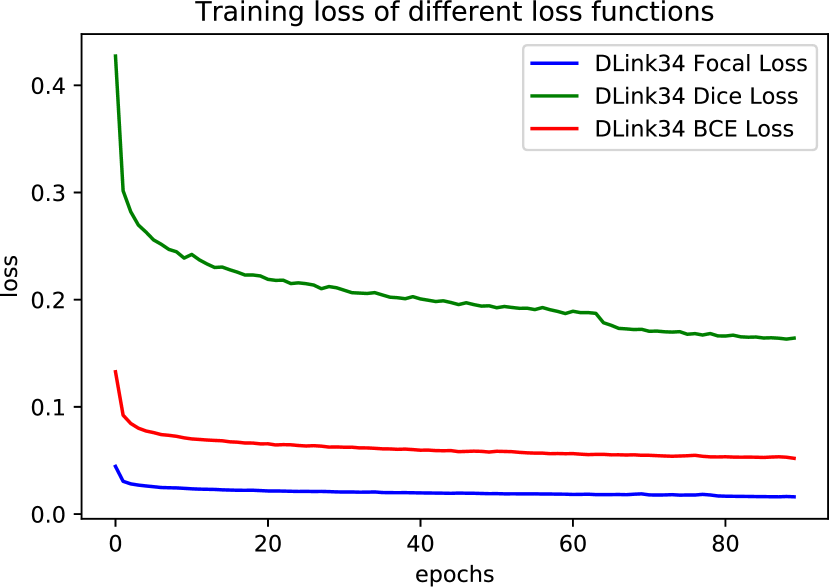
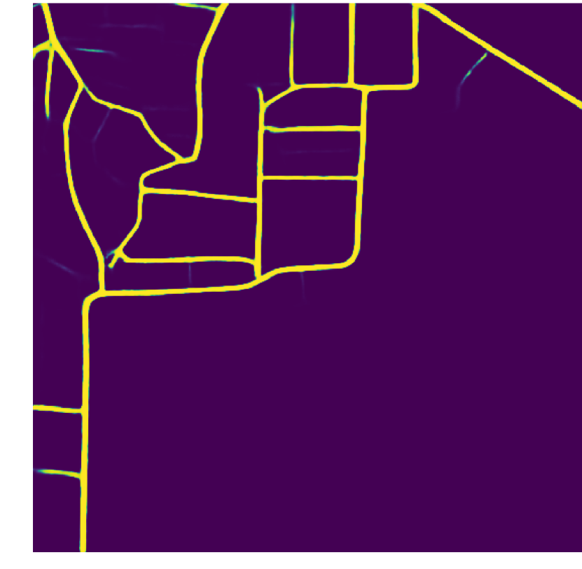
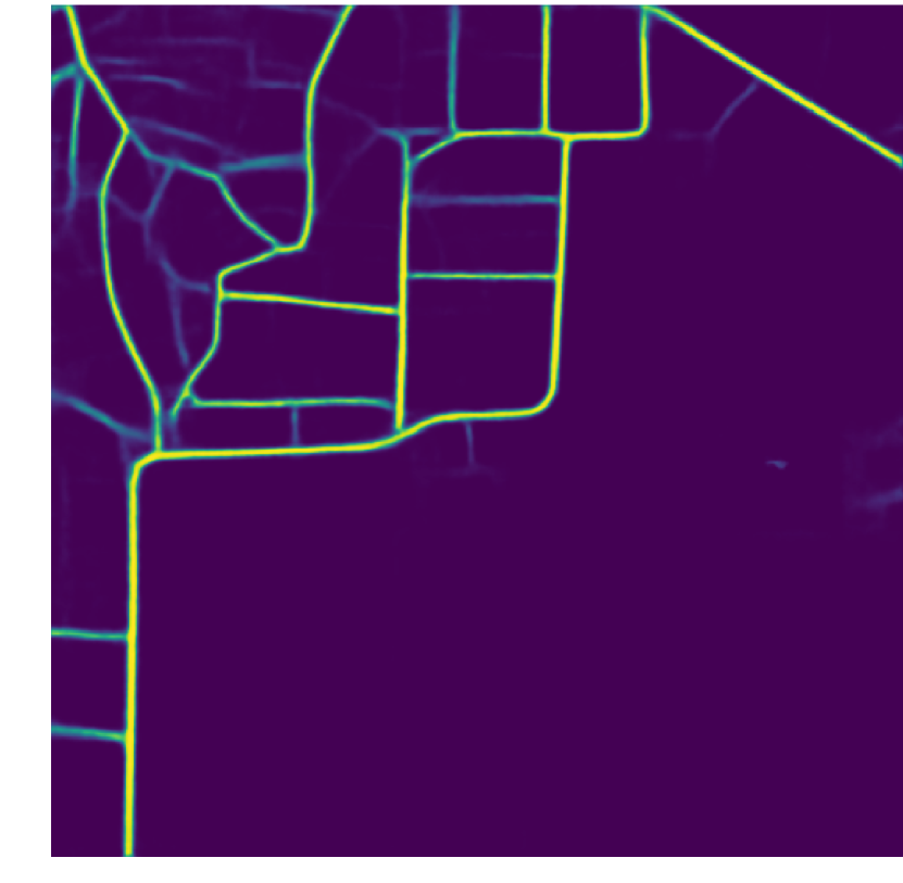
Figure 4(a) shows the training behavior of three loss functions. Interestingly, as can be seen, the focal loss obtains the smallest training loss compared to the BCE and Dice loss. The Dice loss is harder than the BCE and focal loss to be optimized in DLinkNet framework, but it also shows a monotonically decreasing loss values. Table 1 presents meanIOU and APLS scores on test set of Deepglobe road extraction dataset (Demir et al., 2018b). It is consistent with the training loss behaviours that our result for the focal loss model (i.e., 67.82%) is higher the BCE (i.e., 67.21%), and Dice loss model (i.e., 66.31%) respectively. Figure 5 illustrates the difference in confidence map of the BCE+Dice loss model compared to the focal loss model. With the same input image, the BCE+Dice model pays attention to main roads, while the focal loss model is able to put confidence on both main and small roads. This observation is also reflected in APLS scores with a big margin. Our final model with focal loss has improved on the original DLinkNet34(Zhou et al., 2018) with BCE+Dice loss 5.26% on APLS scores (i.e., 77.11% vs. 71.85%). We also argue that APLS score is more important meanIOU score, because it is inherent to connectivity of road network graphs. From following experiments, we use the focal loss for training PP-LinkNet because it is shown as a single effective loss function for the road extraction task.

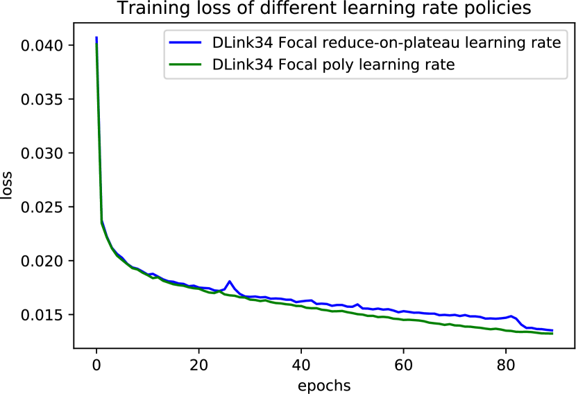
Figure 4(b) shows the training behavior of the poly learning rate policy. The poly learning rate policy is more effective to optimize the deep semantic segmentation system than the reduce-on-plateau learning rate policy. As a result, we improve DLinkNet34 with poly learning rate 1.67% meanIoU from $67.82\%$ to $69.49\%$. We will use the poly learning rate for the following experiments.

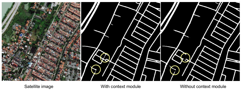
Additionally, Table 1 shows the result of PP-LinkNet34 model with pyramid pooling (PP) context module is better than D-LinkNet34 model with dilation context module (i.e., 69.87% vs. 69.49% in meanIoU, 76.04% vs. 75.71% in APLS). Compared to the original D-LinkNet34, we obtain a larger margin of performance (i.e., 69.87% vs. 67.42% in meanIoU, 76.04% vs. 71.85%) and it suggests that other proposed modifications also have compound effects with the pyramid pooling context module. In other experiments in SpaceNet road network and building footprint dataset (see Table 2, 3), our PP context module also has consistently better performance than dilation context module. Figure 6 shows that our context module can help PP-LinkNet to infer road segments that are difficult to predict when PP-LinkNet does not have the context module.

Finally, our two-stage training further boost performance of the network especially in terms of APLS scores. PP-LinkNet two-stage improves on the first-stage one 3.34% in APLS scores (i.e., 77.11% vs. 73.77%), and also achieve the best results over all model variations.

Figure 6. The impact of the pyramid pooling context module in PP-LinkNet. Left: an input image; middle: the road segmentation mask with PP-Linknet; right: the segmentation mask without the context module in PP-LinkNet. Best viewed in color.

Method	SpaceNet	DeepGlobe
	mIOU  APLS	mIOU  APLS
DeepRoadMapper (segmentation) (Mattyus et al., 2017)	59.99  54.25	62.58  65.56
DeepRoadMapper (full) (Mattyus et al., 2017)	N/A  50.59	N/A  61.66
RoadCNN (segmentation) (Bastani et al., 2018)	62.34  58.41	67.61  69.65
MatAN (Mattyus and Urtasun, 2018)	52.86  46.44	46.88  47.15
Topology Loss (with BCE) (Mosinska et al., 2018)	56.29  49.00	64.95  56.91
Topology Loss (with SoftIoU) (Mosinska et al., 2018)	57.69  51.99	64.94  65.96
LinkNet34 (Chaurasia and Culurciello, 2017)	60.33  55.69	62.75  65.33
D-LinkNet34 (Zhou et al., 2018) (Ours reproduced)	55.50  64.74	67.42  71.86
Improved road connectivity (Batra et al., 2019)	63.75  63.65	67.21  73.12
Self-supervision Coach Mask (Singh et al., 2018)	77.0  N/A	76.8  N/A
Sat2Graph (He et al., 2020)	N/A  64.43	N/A  N/A
PP-LinkNet34 (Ours)	55.50  65.94	69.87  76.04
PP-LinkNet34 two-stage (Ours)	56.43  67.03	70.53  77.11

Table 2. Our results of our PP-LinkNet models on the road network extraction task, and comparison of our technique with the state-of-the-art road network extraction techniques on SpaceNet and DeepGlobe road extraction dataset.

Method	meanIoU	F1 score
	(%)	(%)
PP-LinkNet34 two-stage (Ours)	78.19	68.92
PP-LinkNet34 first-stage (OSM data)	44.00	25.33
PP-LinkNet34 (Ours)	76.62	67.04
DLinkNet34 (Zhou et al., 2018) (Ours reproduced)	76.21	66.79

Table 3. Results of our PP-LinkNet model on building footprint detection task. Top half: different variations of our PP-LinkNet; Bottom half: our reproduced results from other works.

Road network extraction. Table 2 shows our results on SpaceNet and DeepGlobe road extraction dataset. With our two-stage training, we are able to improve quantitative metrics over PP-LinkNet one-stage training over two datasets. We achieve larger gaps of improvements in APLS scores in both dataset. APLS score involves topological measures, hence, it means that our two-stage approach boosts the ability of PP-LinkNet to detect road connectivity.

Furthermore, Table 2 also shows that our PP-LinkNet obtains the new state-of-the-art performance on both SpaceNet and DeepGlobe dataset. Notice that SpaceNet road dataset does not have pixel-level annotations, hence, its meanIOU evaluation based on the assumption that all roads have a fixed road width, which is often not true. Batra et al. (Batra et al., 2019) proposed a method to learn road orientation at the same time with segmentation, and used it to refine connectivity of roads. Despite that, we outperform (Batra et al., 2019) with regard to APLS scores in both dataset (i.e., 3.38% in SpaceNet (67.03% vs. 63.65%), 3.99% in DeepGlobe (77.11% vs. 73.12%)). We also outperform other popular techniques for road network extraction such as DeepRoadMapper(Mattyus et al., 2017), D-LinkNet(Zhou et al., 2018), RoadTracer(Bastani et al., 2018) etc. Furthermore, our result is also better than the recent Sat2Graph (He et al., 2020) technique on SpaceNet dataset.

Figure 7. Examples of building footprint extraction from SpaceNet building dataset. We only use 3 channels R, G, B among multi-spectral imagery to train and test our model. From top to bottom: overlaid image between segmentation mask and RGB input image, segmentation mask, and ground truth image.

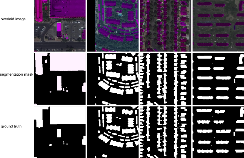
Building footprint extraction. Table 3 shows our results on building footprint extraction tasks. As can be observed, our PP-LinkNet two-stage out-performs all other variations in both meanIOU and F1 score at IOU of 0.5. Similarly to the road extraction problem, our PP-LinkNet first-stage does not show good quantitative results because the rasterized OSM pseudo ground truth is not accurate pixel-to-pixel matching between mask and satellite imagery. Our PP-LinkNet two-stage also performs better than PP-LinkNet one-stage (i.e., 78.19% vs. 76.62% in meanIoU, 68.92% vs. 67.04% in F1 score). Our work is the first work that evaluates our models on SpaceNet building footprint dataset. Hence, it is hard to compare with other existing models (Hamaguchi and Hikosaka, 2018; Golovanov et al., 2018; Iglovikov et al., 2018). We have better performance than our reproduced DLinkNet34 (Zhou et al., 2018), and it indicates that pyramid pooling module captures global scene context better than DLinkNet34’s context module. We don’t have training script for TernausNetV2 (Iglovikov et al., 2018) trained on both our train and test set, therefore, its released model’s result would approximate the upper-bound performance on the dataset (i.e., 76.76% in F1 score). Furthermore, our PP-LinkNet model has performance on par with the winner of SpaceNet building detection (i.e., F1=69%), although we don’t use multi-spectral channels and ensembles of multiple deep learning models. Figure 7 demonstrates some visualizations of our segmentation result mask. It shows that our model can pick out building footprint reasonably well (i.e., third column in Figure 7).

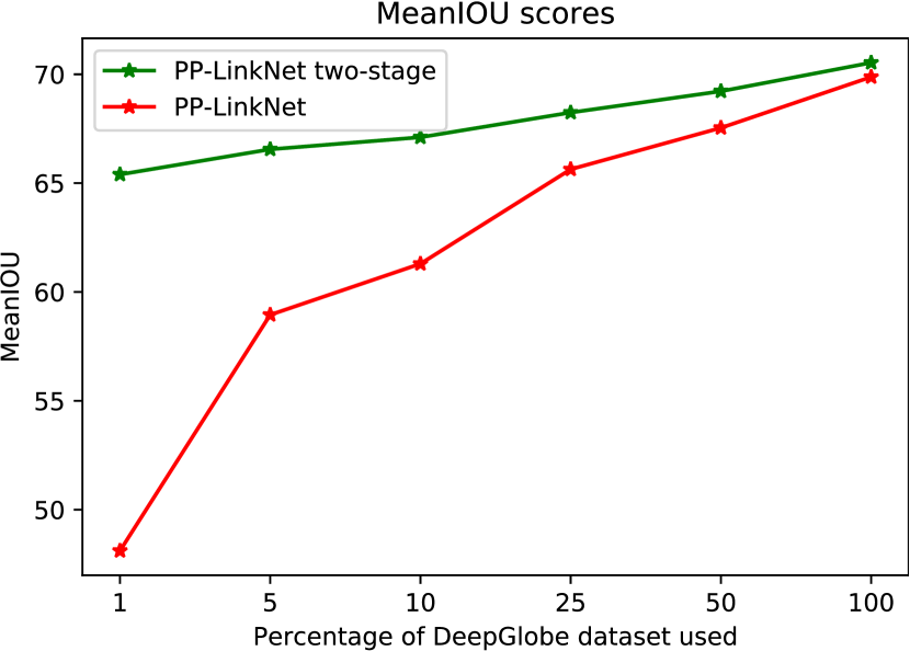
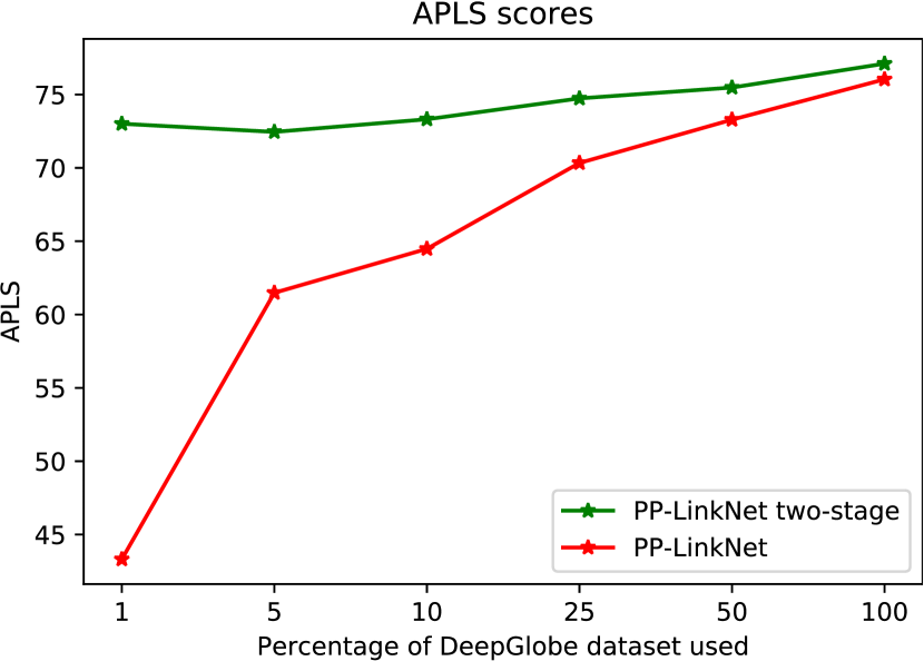
Transfer learning on small data. Figure 8 demonstrates the effects of our two-stage transfer learning for semantic segmentation in the road extraction task. We vary the fraction of DeepGlobe road extraction dataset for training our PP-LinkNet model by selecting randomly 1%(i.e., equivalently to 46 samples), 5%, 10%, 25%, 50% and 100% subset of the dataset. Our PP-LinkNet two-stage performance is better than PP-LinkNet by a large margin in the extremely low number of training samples (e.g., 1%, 5%). The gap of performances is gradually reduced when we have more training samples. In this experiment, we show that our two-stage training procedure helps transfer learning to be more effective in learning visual representations from a small number of satellite images.

(a) MeanIOU scores

(b) APLS scores

Figure 8. Performance of PP-LinkNet two-stage training compared with PP-LinkNet in term of meanIOU and APLS score with respect to the fraction of DeepGlobe road dataset used for training the model. Best viewed in color.

6. Discussions

Domain adaptation is an important procedure for adapting the models of supervised learning into domains different with the trained environment. Often, the new domain (e.g., aerial, medical imagery) has small data or small annotated data. Our two-stage transfer learning is beneficial in adapting supervised learning trained with big data into new domains with small data.

Our two-stage transfer learning is also closely related to training deep learning models in the revival era of deep learning (Hinton et al., 2006). At that time, we pre-train each layer of Restricted Boltzmann Machine in unsupervised fashion, and then, we fine-tune the whole network for different tasks. In our work, with the prevalence of supervised learning techniques, computing resources, and data, we first pre-train the whole deep model on pseudo-groundtruth (noisy) data, then fine-tune it on high-quality annotated data.

7. Conclusion

This paper introduces a new procedure to generate and utilize per-pixel pseudo ground truth labels for extracting road network and building footprint in satellite images. The procedure would allow us to fine-tune semantic segmentation systems on less amount of annotated satellite imagery. Furthermore, we show the new state-of-the-art evaluation results of our PP-LinkNet system on three challenging remote sensing datasets.

References

- (1)
- Dic ([n.d.]) [n.d.]. https://wikipedia.org/wiki/Sorensen–Dice_coefficient.
- Audebert et al. (2017) Nicolas Audebert, Bertrand Le Saux, and Sebastien Lefevre. 2017. Joint Learning From Earth Observation and OpenStreetMap Data to Get Faster Better Semantic Maps. In The IEEE Conference on Computer Vision and Pattern Recognition (CVPR) Workshops.
- Badrinarayanan et al. (2017) Vijay Badrinarayanan, Alex Kendall, and Roberto Cipolla. 2017. SegNet: A Deep Convolutional Encoder-Decoder Architecture for Image Segmentation. IEEE Transactions on Pattern Analysis and Machine Intelligence 39, 12 (2017), 2481–2495. https://doi.org/10.1109/TPAMI.2016.2644615 arXiv:1511.00561
- Bastani et al. (2018) Favyen Bastani, Songtao He, Sofiane Abbar, Mohammad Alizadeh, Hari Balakrishnan, Sanjay Chawla, Sam Madden, and David DeWitt. 2018. RoadTracer: Automatic Extraction of Road Networks from Aerial Images. (2018). https://doi.org/10.1109/CVPR.2018.00496 arXiv:1802.03680
- Batra et al. (2019) Anil Batra, Suriya Singh, Guan Pang, Saikat Basu, C V Jawahar, and Manohar Paluri. 2019. Improved Road Connectivity by Joint Learning of Orientation and Segmentation. In The IEEE Conference on Computer Vision and Pattern Recognition (CVPR).
- Bulo et al. (2018) Samuel Rota Bulo, Lorenzo Porzi, and Peter Kontschieder. 2018. In-place Activated BatchNorm for Memory-Optimized Training of DNNs. In Proceedings of the IEEE Computer Society Conference on Computer Vision and Pattern Recognition. 5639–5647. https://doi.org/10.1109/CVPR.2018.00591 arXiv:1712.02616
- Chaurasia and Culurciello (2017) Abhishek Chaurasia and Eugenio Culurciello. 2017. LinkNet: Exploiting encoder representations for efficient semantic segmentation. In IEEE Visual Communications and Image Processing (VCIP). https://doi.org/10.1109/VCIP.2017.8305148 arXiv:1707.03718
- Chen et al. (2018) Liang Chieh Chen, George Papandreou, Iasonas Kokkinos, Kevin Murphy, and Alan L. Yuille. 2018. DeepLab: Semantic Image Segmentation with Deep Convolutional Nets, Atrous Convolution, and Fully Connected CRFs. IEEE Transactions on Pattern Analysis and Machine Intelligence 40, 4 (2018), 834–848. https://doi.org/10.1109/TPAMI.2017.2699184 arXiv:1606.00915
- Demir et al. (2018a) Ilke Demir, Forest Hughes, Aman Raj, Kaunil Dhruv, Suryanarayana Murthy Muddala, Sanyam Garg, Barrett Doo, and Ramesh Raskar. 2018a. Generative Street Addresses from Satellite Imagery. ISPRS International Journal of Geo-Information 7, 3 (2018). https://doi.org/10.3390/ijgi7030084
- Demir et al. (2018b) Ilke Demir, Krzysztof Koperski, David Lindenbaum, Guan Pang, Jing Huang, Saikat Basu, Forest Hughes, Devis Tuia, and Ramesh Raska. 2018b. DeepGlobe 2018: A challenge to parse the earth through satellite images. In IEEE Conference on Computer Vision and Pattern Recognition Workshops (CVPRW). https://doi.org/10.1109/CVPRW.2018.00031 arXiv:1805.06561
- Deng et al. (2009) J Deng, W Dong, R Socher, L.-J. Li, K Li, and L Fei-Fei. 2009. ImageNet: A Large-Scale Hierarchical Image Database. In The IEEE Conference on Computer Vision and Pattern Recognition (CVPR).
- Everingham et al. (2010) M Everingham, L Van~Gool, C K I Williams, J Winn, and A Zisserman. 2010. The Pascal Visual Object Classes (VOC) Challenge. International Journal of Computer Vision 88, 2 (2010), 303–338.
- Golovanov et al. (2018) Sergey Golovanov, Rauf Kurbanov, Aleksey Artamonov, Alex Davydow, and Sergey Nikolenko. 2018. Building detection from satellite imagery using a composite loss function. In IEEE Computer Society Conference on Computer Vision and Pattern Recognition Workshops. https://doi.org/10.1109/CVPRW.2018.00040
- Hamaguchi and Hikosaka (2018) Ryuhei Hamaguchi and Shuhei Hikosaka. 2018. Building Detection From Satellite Imagery Using Ensemble of Size-Specific Detectors. In The IEEE Conference on Computer Vision and Pattern Recognition (CVPR) Workshops.
- He et al. (2017) Kaiming He, Georgia Gkioxari, Piotr Dollár, and Ross Girshick. 2017. Mask R-CNN. (mar 2017). arXiv:1703.06870 http://arxiv.org/abs/1703.06870
- He et al. (2016) Kaiming He, Xiangyu Zhang, Shaoqing Ren, and Jian Sun. 2016. Deep residual learning for image recognition. In Proceedings of the IEEE Computer Society Conference on Computer Vision and Pattern Recognition, Vol. 2016-Decem. 770–778. https://doi.org/10.1109/CVPR.2016.90 arXiv:1512.03385
- He et al. (2020) Songtao He, Favyen Bastani, Satvat Jagwani, Mohammad Alizadeh, Hari Balakrishnan, Sanjay Chawla, Mohamed M. Elshrif, Samuel Madden, and Amin Sadeghi. 2020. Sat2Graph: Road Graph Extraction through Graph-Tensor Encoding. (jul 2020). arXiv:2007.09547 http://arxiv.org/abs/2007.09547
- Hinton et al. (2006) Geoffrey E. Hinton, Simon Osindero, and Yee Whye Teh. 2006. A fast learning algorithm for deep belief nets. Neural Computation 18, 7 (2006), 1527–1554. https://doi.org/10.1162/neco.2006.18.7.1527
- Humanitarian OpenStreetMap Team ([n.d.]) Humanitarian OpenStreetMap Team. [n.d.]. https://export.hotosm.org/en/v3/. https://export.hotosm.org/en/v3/
- Iglovikov et al. (2018) Vladimir Iglovikov, Selim Seferbekov, Alexander Buslaev, and Alexey Shvets. 2018. TernausNetV2: Fully convolutional network for instance segmentation. In IEEE Conference on Computer Vision and Pattern Recognition Workshops (CVPRW). 228–232. https://doi.org/10.1109/CVPRW.2018.00042 arXiv:1806.00844
- Lin et al. (2017) Tsung-Yi Lin, Piotr Dollár, Ross Girshick, Kaiming He, Bharath Hariharan, and Serge Belongie. 2017. Feature Pyramid Networks for Object Detection. In CVPR. arXiv:1612.03144 http://arxiv.org/abs/1612.03144
- Lin et al. (2014) Tsung Yi Lin, Michael Maire, Serge Belongie, James Hays, Pietro Perona, Deva Ramanan, Piotr Dollár, and C. Lawrence Zitnick. 2014. Microsoft COCO: Common objects in context. In European Conference on Computer Vision, Vol. 8693 LNCS. 740–755. https://doi.org/10.1007/978-3-319-10602-1_48 arXiv:1405.0312
- Liu et al. (2016) Wei Liu, Andrew Rabinovich, and Alexander C. Berg. 2016. ParseNet: Looking Wider to See Better. ICLR (jun 2016). arXiv:1506.04579 http://arxiv.org/abs/1506.04579
- Luo et al. (2015) Ye Luo, Loong-Fah Cheong, and An Tran. 2015. Actionness-assisted Recognition of Actions. In The IEEE International Conference on Computer Vision (ICCV).
- Mattyus et al. (2017) Gellert Mattyus, Wenjie Luo, and Raquel Urtasun. 2017. DeepRoadMapper: Extracting Road Topology From Aerial Images. In The IEEE International Conference on Computer Vision (ICCV).
- Mattyus and Urtasun (2018) Gellert Mattyus and Raquel Urtasun. 2018. Matching Adversarial Networks. In The IEEE Conference on Computer Vision and Pattern Recognition (CVPR).
- Mattyus et al. (2015) Gellert Mattyus, Shenlong Wang, Sanja Fidler, and Raquel Urtasun. 2015. Enhancing Road Maps by Parsing Aerial Images Around the World. In International Conference on Computer Vision (ICCV).
- Milletari et al. (2016) Fausto Milletari, Nassir Navab, and Seyed Ahmad Ahmadi. 2016. V-Net: Fully convolutional neural networks for volumetric medical image segmentation. Proceedings - 2016 4th International Conference on 3D Vision, 3DV 2016 (2016), 565–571. https://doi.org/10.1109/3DV.2016.79 arXiv:1606.04797
- Mosinska et al. (2018) Agata Mosinska, Pablo Marquez-Neila, Mateusz Kozinski, and Pascal Fua. 2018. Beyond the Pixel-Wise Loss for Topology-Aware Delineation. In Proceedings of the IEEE Computer Society Conference on Computer Vision and Pattern Recognition. 3136–3145. https://doi.org/10.1109/CVPR.2018.00331 arXiv:1712.02190
- Narang et al. (2018) Sharan Narang, Gregory Diamos, Erich Elsen, Paulius Micikevicius, Jonah Alben, David Garcia, Boris Ginsburg, Michael Houston, Oleksii Kuchaiev, Ganesh Venkatesh, and Hao Wu. 2018. Mixed precision training. In 6th International Conference on Learning Representations, ICLR 2018 - Conference Track Proceedings. arXiv:1710.03740 http://arxiv.org/abs/1710.03740
- Neuhold et al. (2017) Gerhard Neuhold, Tobias Ollmann, Samuel Rota Bulò, and Peter Kontschieder. 2017. The Mapillary Vistas Dataset for Semantic Understanding of Street Scenes. In International Conference on Computer Vision (ICCV). https://www.mapillary.com/dataset/vistas
- Paszke et al. (2016) Adam Paszke, Abhishek Chaurasia, Sangpil Kim, and Eugenio Culurciello. 2016. ENet: A Deep Neural Network Architecture for Real-Time Semantic Segmentation. (2016). arXiv:1606.02147 http://arxiv.org/abs/1606.02147
- Ren et al. (2015) Shaoqing Ren, Kaiming He, Ross Girshick, and Jian Sun. 2015. Faster R-CNN: Towards Real-Time Object Detection with Region Proposal Networks. (jun 2015). arXiv:1506.01497 http://arxiv.org/abs/1506.01497
- Ronneberger et al. (2015) Olaf Ronneberger, Philipp Fischer, and Thomas Brox. 2015. U-net: Convolutional networks for biomedical image segmentation. Lecture Notes in Computer Science (including subseries Lecture Notes in Artificial Intelligence and Lecture Notes in Bioinformatics) 9351 (2015), 234–241. https://doi.org/10.1007/978-3-319-24574-4_28 arXiv:1505.04597
- Shelhamer et al. (2015) Evan Shelhamer, Jonathan Long, and Trevor Darrell. 2015. Fully Convolutional Networks for Semantic Segmentation. In IEEE Conference on Computer Vision and Pattern Recognition, Vol. 39. 640–651. https://doi.org/10.1109/TPAMI.2016.2572683 arXiv:1411.4038
- Singh et al. (2018) Suriya Singh, Anil Batra, Guan Pang, Lorenzo Torresani, Saikat Basu, Manohar Paluri, and C. V. Jawahar. 2018. Self-supervised Feature Learning for Semantic Segmentation of Overhead Imagery. In British Machine Vision Conference (BMVC), Vol. 1.
- Tran and Cheong (2017) An Tran and Loong-Fah Cheong. 2017. Two-stream Flow-guided Convolutional Attention Networks for Action Recognition. In The IEEE International Conference on Computer Vision Workshop (ICCVW).
- USGS ([n.d.]) USGS. [n.d.]. https://earthexplorer.usgs.gov/. https://earthexplorer.usgs.gov/
- Van Etten et al. (2018) Adam Van Etten, Dave Lindenbaum, and Todd M. Bacastow. 2018. SpaceNet: A Remote Sensing Dataset and Challenge Series. (2018). arXiv:1807.01232 http://arxiv.org/abs/1807.01232
- Wang et al. (2018) Panqu Wang, Pengfei Chen, Ye Yuan, Ding Liu, Zehua Huang, Xiaodi Hou, and Garrison Cottrell. 2018. Understanding Convolution for Semantic Segmentation. In IEEE Winter Conference on Applications of Computer Vision (WACV). 1451–1460. https://doi.org/10.1109/WACV.2018.00163 arXiv:1702.08502
- Wang et al. (2017) Shenlong Wang, Min Bai, Gellert Mattyus, Hang Chu, Wenjie Luo, Bin Yang, Justin Liang, Joel Cheverie, Sanja Fidler, and Raquel Urtasun. 2017. TorontoCity: Seeing the World with a Million Eyes. In Proceedings of the IEEE International Conference on Computer Vision. https://doi.org/10.1109/ICCV.2017.327 arXiv:1612.00423
- Zhao et al. (2017) Hengshuang Zhao, Jianping Shi, Xiaojuan Qi, Xiaogang Wang, and Jiaya Jia. 2017. Pyramid scene parsing network. In IEEE Conference on Computer Vision and Pattern Recognition (CVPR). https://doi.org/10.1109/CVPR.2017.660 arXiv:1612.01105v2
- Zhou et al. (2018) Lichen Zhou, Chuang Zhang, and Ming Wu. 2018. D-linknet: Linknet with pretrained encoder and dilated convolution for high resolution satellite imagery road extraction. In IEEE Computer Society Conference on Computer Vision and Pattern Recognition Workshops, Vol. 2018-June. https://doi.org/10.1109/CVPRW.2018.00034