Low rank tensor approximation of singularly perturbed partial differential equations in one dimension

Abstract.

We derive rank bounds on the quantized tensor train (QTT) compressed approximation of singularly perturbed reaction diffusion partial differential equations (PDEs) in one dimension. Specifically, we show that, independently of the scale of the singular perturbation parameter, a numerical solution with accuracy $0<\varepsilon<1$ can be represented in QTT format with a number of parameters that depends only polylogarithmically on $\varepsilon$. In other words, QTT compressed solutions converge exponentially to the exact solution, with respect to a root of the number of parameters. We also verify the rank bound estimates numerically, and overcome known stability issues of the QTT based solution of PDEs by adapting a preconditioning strategy to obtain stable schemes at all scales. We find, therefore, that the QTT based strategy is a rapidly converging algorithm for the solution of singularly perturbed PDEs, which does not require prior knowledge on the scale of the singular perturbation and on the shape of the boundary layers.

1. Introduction

The solution of singularly perturbed elliptic differential equations constitutes a challenge for numerical approximation. The solutions to such problems exhibit boundary layers, whose correct resolution is crucial to the accurate approximation of the problem. Since those layers can get arbitrarily small, and the variations in the gradient of the solution can get consequentially highly concentrated in space, the accurate solution of singularly perturbed problems, by, e.g., low-order finite element (FE) methods requires a computationally demanding number of degrees of freedom. For this reason, more effective methods have been introduced, such as $hp$-FE methods [SS96], see also [Sch98, Chapter 3] and [Mel02], where some a priori knowledge on the solution is exploited to construct numerical methods requiring a smaller computational effort. In some instances, especially in high dimension, the implementation of such methods can still be cumbersome.

In this paper, we discuss and analyze the numerical solution of one-dimensional, singularly perturbed elliptic equations in tensor-compressed format. Specifically, we formally approximate the problem using low order, piecewise linear finite elements and compress the resulting algebraic problem (neither the right-hand side, nor the matrix of this system are formed explicitly in computations) using the quantized tensor train (QTT) method [Ose10, Kho11]. By doing this, we obtain an approximation accuracy comparable with that of a low-order finite element on a very fine grid (the so-called virtual grid), but we only need a significantly smaller number of degrees of freedom to compute and represent the solution. We also remark that the QTT based approach to the solution of singularly perturbed problems does not require a priori knowledge on the scale of the singular perturbation, nor on the explicit form of the layers, as for, e.g., enriched spectral methods [CHT20].

1.1. Contributions of this paper

First, we show theoretically and verify numerically that, for all $0<\varepsilon<1$, we can obtain a QTT approximation of the solution with accuracy $\varepsilon>0$, and that we can represent it with $\mathcal{O}(\left|\log\varepsilon\right|^{\kappa})$ parameters, with $\kappa=3$. For a given accuracy, the number of parameters of the QTT approximation is independent of the singular perturbation parameter. This is the main theoretical contribution of this paper, and it is stated in Theorem 1. Furthermore, this is a theoretical upper bound: we find, in numerical experiments, that $\kappa$ can be smaller in practice.

The second contribution of this paper is the adaptation of the preconditioner introduced in [BK20] to the singularly perturbed case. The straightforward application of classic solvers (DMRG [Whi92], AMEn [DS14], etc.) to the QTT formatted tends indeed to have stability issues, which greatly limit the virtual grid sizes that can be used in practice. In [BK20], a BPX preconditioner was developed to overcome this issue; we adapt it to our case, in order to obtain stable solutions for all values of the perturbation parameter $0<\delta<1$. With this at hand, we are able to reach a virtual grid size of around $2^{-50}$ and to accurately solve problems with $\delta=10^{-16}$. We remark that such an approximation, if represented as a full piecewise linear FE function, would require approximately $10^{15}$ degrees of freedom, while it is easily tractable in tensor-compressed, QTT format.

1.2. Tensor compressed solution of PDEs

Historically, the first appearance of tensor decomposition dates back to F. Hitchcook in [Hit27]. In more recent years, a wide range of tensor decompositions have appeared and have been applied to many fields of science and engineering, see [KB09]. The tensor train (TT) decomposition, specifically, was introduced in [Ose11a] as an easy to construct low-rank decomposition of high-dimensional matrices and has its roots in matrix product states representations in physics [Sch11]. Shortly later, it was realized that low-rank tensor representations can handle certain low-dimensional partial differential equation (PDEs) that exhibit rough behavior and are computationally challenging for conventional methods, through so-called quantization. This refers to the process of reshaping low-dimensional tensors with high mode sizes into high-dimensional tensor with small mode size, then applying tensor decomposition. By combining quantization and the TT representation, one obtains the QTT representation.

The QTT-formatted solution of PDEs proves useful only if the tensors involved have small QTT-ranks: to theoretically analyse the rank behavior in the problem under consideration, we approximate the solution with high-order piecewise polynomials, then $L^{2}$-project the resulting approximation into the low-order piecewise linear finite element space. We can then show that the FE function thus constructed has low exact QTT-ranks (specifically, QTT-ranks that grow only linearly with respect to the polynomial degree of the high-degree approximation). The strategy used here is then partially different from the approach in [KS18, MRS19], where the high-order piecewise polynomial was interpolated. $L^{2}$-projections have the advantage, with respect to interpolation operators, of being stable with respect to the $\delta$-dependent norm we compute the error in. It is worth noting that, while the analysis in multiple dimensions can be significantly more complex than the one presented here, the strategy to obtain rank bounds can be extended to the multi-dimensional case.

1.3. Structure of the paper

In Section 2 we introduce the singularly perturbed problem and the functional setting of the paper. Section 3 contains the main theoretical findings of this paper, i.e., the rank bounds and error analysis for QTT compressed solution of the singularly perturbed problem. Specifically, we show in Theorem 1 that the number of parameters of the QTT representation of the solution grows only polylogarithmically with respect to the approximation error. In Section 4 we discuss the numerical stability of the QTT formatted problem and propose a preconditioning strategy whose implementation details are deferred to Appendix A. Finally, in Section 5 we present numerical experiments to verify the theoretical results obtained in Section 3 and the role of preconditioning. We conclude and discuss extensions of the present work in Section 6.

2. Statement of the problem and notation

2.1. Statement of the problem

We consider the following problem on the interval $I=(0,1)$

(1) $$-\delta^{2}u_{\delta}^{\prime\prime}+cu_{\delta}=f\text{ in }I,$$

$$u_{\delta}(0)=\alpha_{0},\,u_{\delta}(1)=\alpha_{1},$$

where $0<\delta<1$, $\alpha_{1},\alpha_{0}\in\mathbb{R}$, and where

(2) $$f\text{ and }c\text{ are analytic in }\bar{I}=[0,1]\text{ and }c(x)\geq c_{\min{}}>0,\,\forall x\in I.$$

For the weak formulation of problem (LABEL:DiffEq), we introduce the Sobolev spaces

$$H^{1}(I)\coloneqq\left\{u\in L^{2}(I):u^{\prime}\in L^{2}(I)\right\},\qquad H^{1}_{0}(I)\coloneqq\left\{u\in H^{1}(I):u(0)=u(1)=0\right\},$$

and

$$H^{1}_{D}(I)\coloneqq\left\{u\in H^{1}(I):u(0)=\alpha_{0},u(1)=\alpha_{1}\right\}.$$

The weak formulation of (LABEL:DiffEq) reads then: find $u_{\delta}\in H^{1}_{D}(I)$ such that

(3) $$a_{\delta}(u_{\delta},v)\coloneqq\int_{I}\delta^{2}u_{\delta}^{\prime}v^{\prime}+\int_{I}cu_{\delta}v=\int_{I}fv,\quad\forall v\in H^{1}_{0}(I),$$

By Lax-Milgram’s theorem, for all $\delta>0$, problem (3) is well defined and has a unique solution. We introduce, on $H^{1}(I)$, the $\delta$-dependent norm

(4) $$||v||_{\delta}:=\big{(}\delta^{2}||v^{\prime}||_{L^{2}(I)}^{2}+||v||_{L^{2}(I)}^{2}\big{)}^{1/2}.$$

We do our analysis in the energy norm just introduced. In the literature, the stronger, balanced norm is sometimes instead considered, see [MX16]. An analysis in this norm is out of the scope of the present paper.

2.2. Notation

We write $\mathbb{N}=\{1,2,\dots\}$ for the set of positive natural numbers and $\mathbb{N}_{0}=\mathbb{N}\cup\{0\}$. For $p\in\mathbb{N}_{0}$ and $\Omega\subset\mathbb{R}$, let $\mathbb{P}_{p}(\Omega)$ denote the space of polynomials of degree at most $p$ defined on $\Omega$.

We use the convention that capitalized letters are used for multidimensional arrays and non-capitalized letters are used for vectors.

Throughout, if not stated otherwise, we use the convention that $C>0$ denotes a generic constant independent of the singular perturbation parameters $\delta$ and of the discretization. $C$ may change value without notice.

With the word tensor we indicate multidimensional arrays: a general $d$-dimensional tensor is an element $A\in\mathbb{R}^{n_{1}\times\ldots n_{d}}$, with $n_{i}\in\mathbb{N}$ for $i=1,\ldots,d$, and requires storage of order $\mathcal{O}(n_{1}\cdot\ldots\cdot n_{d})$.

3. Low rank QTT approximation

In this section, we develop the error analysis and the rank bounds for the low-rank QTT-formatted approximation of the solutions to (LABEL:DiffEq). We construct the low-rank representation of solutions $u_{\delta}$ to (LABEL:DiffEq) by constructing a piecewise, high-order polynomial approximation to $u_{\delta}$, then reapproximating it in a low-order finite element space, and finally QTT compressing the resulting vector of coefficients.

We start by introducing the TT and QTT representations in Section 3.1. In Section 3.2, then, we introduce the high-order and the low-order finite element spaces. Finally, we derive rank bounds and estimate the approximation error in Sections 3.3 and 3.4, respectively.

3.1. Quantized Tensor Train

We now formalize the concepts of tensor trains [Ose11a] and quantized tensor trains.

Definition 1.

A $d$-dimensional tensor $A\in\mathbb{R}^{\overbrace{\scriptstyle{n\times\ldots\times n}}^{d\text{ times}}}$ is said to admit a TT-decomposition if there exist $\{r_{j}\}_{j=0}^{d}\in\mathbb{N}^{d+1}$ such that $r_{0}=r_{d}=1$ and that there exists, for all $j\in\{1,\dots,d\}$, $V^{j}:\{0,\dots,n-1\}\to\mathbb{R}^{r_{j-1}\times r_{j}}$ such that

(5) $$A(i_{1},\ldots,i_{d})=V^{1}(i_{1})\ldots V^{d}(i_{d}),\qquad\forall(i_{1},\dots,i_{d})\in\{0,\dots,n-1\}^{d},$$

The tensors $V^{j}$, seen as elements of $\mathbb{R}^{r_{j-1}\times n\times r_{j}}$, are the TT-cores of the decomposition, while $\{r_{j}\}_{j=1}^{d-1}$ are the TT-ranks of the decomposition.

We assume that $r_{2},\ldots,r_{d-1}=r\in\mathbb{N}$, for ease of presentation. The storage required for the representation in (5) is of order $\mathcal{O}(nr^{2}d)$, as each $V^{j}$ can be regarded as a $3$-tensor in $\mathbb{R}^{r\times n\times r}$ and there are $d$ such elements. The storage requirement of a $d$-tensor $A\in\mathbb{R}^{n\times\ldots\times n}$ in the TT-format is polynomial in the dimension $d$, provided the TT-ranks satisfy $r\leq Cd^{k}$ for some $C,k>0$ independent of $d$, instead of the exponential dependence $\mathcal{O}(n^{d})$ on $d$ of storage of a tensor represented as a $d$-dimensional array.

We now introduce the quantized tensor train (QTT) format. Let $u\in\mathbb{R}^{2^{L}}$, for $L\in\mathbb{N}$, and assume it is indexed by $i=0,\ldots,2^{L}-1$. Any index $i\in\{0,\ldots,2^{L}-1\}$ admits a binary representation; that is, there exist $i_{j}\in\{0,1\}$, for $j=0,\ldots,L-1$, such that

(6) $$i=\sum_{j=1}^{L}2^{L-j}i_{j}.$$

We define, using the representation in equation (6), the $L$-tensor $U\in\mathbb{R}^{2\times\ldots\times 2}$ such that

(7) $$U(i_{1},\ldots,i_{L})\coloneqq u(i),\qquad\forall i=\sum_{j=1}^{L}2^{L-j}i_{j}\in\{0,\dots,2^{L}-1\}$$

Definition 2.

A vector $u\in\mathbb{R}^{2^{L}}$ is said to admit a QTT decomposition [Ose10, Kho11] if the corresponding $L$-tensor $U\in\mathbb{R}^{2\times\ldots\times 2}$ defined in equation (7) admits a TT-decomposition as in Definition 1. The TT-cores of the decomposition of $U$ are called the QTT-cores of the decomposition of $u$ and the TT-ranks of the decomposition of $U$ are called the QTT-ranks of the decomposition of $u$. The storage requirement for such a QTT decomposition is of order $\mathcal{O}(r^{2}L)$ where $r$ is the maximal QTT-rank of the decomposition of $u$.

The setting that we are interested in is when $u\in\mathbb{R}^{2^{L}}$ is the coefficient vector of a finite element (FE) function on a uniform grid. The notion of QTT decompositions can be extended to include functions $f\colon\mathbb{R}\to\mathbb{R}$:

Definition 3.

Let $I\subset\mathbb{R}$ be an open interval, and let $\mathcal{T}=\{x_{1}<\ldots<x_{2^{L}}\}\subset\overline{I}$. A function $f\colon I\to\mathbb{R}$, well defined at the points of $\mathcal{T}$, is said to admit a QTT decomposition with respect to $\mathcal{T}$ if the vector $v\in\mathbb{R}^{2^{L}}$ with elements

$$(v)_{i}=f(x_{i}),\qquad\forall i\in\{1,\dots,2^{L}\},$$

admits a QTT-representation. The QTT-cores of the QTT representation of $v$ are referred to as the QTT-cores of $f$ and the QTT-ranks of the QTT representation of $v$ are referred to as the QTT-ranks of $f$.

Certain functions admit exact decompositions in the QTT format on equispaced grids $\mathcal{T}$, with bounded ranks. Two fundamental examples of such functions are given in Example 1 and Example 2. For $L\in\mathbb{N}$, we denote by

(8) $$\mathcal{T}_{L}\coloneqq\left\{x_{j}=j\frac{1}{2^{L}+1},\,j\in\{0,\dots,2^{L}+1\}\right\}$$

the equispaced grid on $\overline{I}=[0,1]$ with $2^{L}+2$ uniformly spaced grid points. Also, let

(9) $$\mathcal{T}^{\mathrm{int}}_{L}\coloneqq\left\{x_{j}=j\frac{1}{2^{L}+1},\,j\in\{1,\dots,2^{L}\}\right\}$$

Example 1.

The exponential function $e^{-\alpha x}$, for $\alpha\in\mathbb{R}$, admits a QTT decomposition with respect to $\mathcal{T}^{\mathrm{int}}_{L}$ with QTT-ranks $r=1$, where $L\in\mathbb{N}$. Any $x\in\mathcal{T}^{\mathrm{int}}_{L}$, can be written as $x=ih$, for some $i\in\{1,\dots,2^{L}\}$, where $h$ is the step size of $\mathcal{T}^{\mathrm{int}}_{L}$. Expand $i=\sum_{j=1}^{L}2^{L-j}i_{j}$, with $i_{j}\in\{0,1\}$, in its binary representation. Then we obtain

$$e^{-\alpha x}=e^{-\alpha h\big{(}2^{L-1}i_{1}+2^{L-2}i_{2}+\ldots+2^{1}i_{L-1}+2^{0}i_{L}\big{)}}=e^{-\alpha h2^{L-1}i_{1}}\cdots e^{-\alpha hi_{L}},\qquad\forall x\in\mathcal{T}^{\mathrm{int}}_{L},$$

which is a rank-$1$ QTT decomposition.

Example 2.

Any polynomial function $M$ of degree $p$ admits a QTT-representation with respect to $\mathcal{T}^{\mathrm{int}}_{L}$ with QTT-ranks $r=p+1$. See, e.g., [Ose13, Theorem 6] for details on the decomposition and [Kho11] for a proof of this result. A generalization to piecewise polynomials can be found in, e.g., [KS15, Lemma 3.7] and is included in the present manuscript as Lemma 1.

We refer the reader to [Kho18] for a comprehensive presentation of QTT decomposition.

3.2. Piecewise polynomial approximations

Definition 4.

For any collection $\mathcal{T}=\{\xi_{0},\ldots,\xi_{N}:0=\xi_{0}<\xi_{1}<\ldots<\xi_{N}=1\}\subset\bar{I}$ of ordered points of $\bar{I}$ and for a degree $p\in\mathbb{N}_{0}$, we define

$$V(I,p,\mathcal{T}):=\{v\in C(\bar{I}):v_{|_{[\xi_{i-1},\xi_{i}]}}\in\mathbb{P}_{p}([\xi_{i-1},\xi_{i}])\text{ for }i=1,\ldots,N,\ v(0)=\alpha_{0},\,v(1)=\alpha_{1}\},$$

and

$$V_{0}(I,p,\mathcal{T}):=\{v\in C(\bar{I}):v_{|_{[\xi_{i-1},\xi_{i}]}}\in\mathbb{P}_{p}([\xi_{i-1},\xi_{i}])\text{ for }i=1,\ldots,N,\ v(0)=v(1)=0\}.$$

3.2.1. High order finite element approximation

We now introduce high-order finite element approximation result that will be essential for our main result. For all $\kappa>0$, we denote by $\mathcal{T}^{\mathrm{hp}}_{\kappa}=\{\xi_{0},\xi_{1},\xi_{2},\xi_{3}\}$ the collection of points defined by

(10) $$\xi_{0}=0,\quad\xi_{1}=\min\{0.25,\kappa\},\quad\xi_{2}=1-\min\{0.25,\kappa\},\quad\xi_{3}=1$$

Proposition 1 ([Mel02, Proposition 2.2.5]).

Let $u_{\delta}$ be the solution to (LABEL:DiffEq). There exist $C,b,\lambda_{0}>0$ independent of $\delta$ such that for every $\lambda\in(0,\lambda_{0})$ and for all $p\in\mathbb{N}_{0}$, there exists $u_{\delta,p}\in V(I,p,\mathcal{T}_{\lambda p\delta}^{\mathrm{hp}})$ such that

$$\|u_{\delta}-u_{\delta,p}\|_{\delta}\leq Ce^{-bp}.$$

3.2.2. $\mathbb{P}_{1}$ finite element methods

We introduce here, and will use in QTT-compressed computations, a finite element (FE) method, with piecewise linear basis functions. We introduce the finite dimensional low-order FE spaces

$$V^{L}\coloneqq V(I,1,\mathcal{T}_{L})\quad\text{and}\quad V^{L}_{0}\coloneqq V_{0}(I,1,\mathcal{T}_{L}).$$

The discretized version of the weak formulation in equation (3) reads: find $u_{L}\in V^{L}$ such that

(11) $$\int_{I}\delta^{2}u_{L}^{\prime}v^{\prime}+\int_{I}cu_{L}v=\int_{I}fv,\qquad\forall v\in V^{L}_{0}.$$

The problem in equation (11) can be written algebraically as

(12) $$A_{L}w_{L}=f_{L}$$

where

$$A_{L}\coloneqq\delta^{2}S_{L}+R_{L}\in\mathbb{R}^{2^{L}\times 2^{L}},\qquad w_{L},f_{L}\in\mathbb{R}^{2^{L}}.$$

and where $S_{L}\in\mathbb{R}^{2^{L}\times 2^{L}}$ is the stiffness matrix and $R_{L}\in\mathbb{R}^{2^{L}\times 2^{L}}$ is the matrix such that

$$(R_{L})_{ij}=\int_{I}c\varphi_{i}\varphi_{j},\qquad\forall i,j\in\{1,\dots,2^{L}\},$$

with $\{\varphi_{i}\}_{i=1}^{2^{L}}$ being the Lagrange basis associated with $\mathcal{T}^{\mathrm{int}}_{L}$. $A_{L}$ is called the system matrix and $f_{L}$ is called the load vector of the system in (11). See, e.g., [EG04, BS08] for more details on finite element methods.

Let us now introduce the $\mathbb{P}_{1}$-FE Galerkin projection $\Pi_{L}\colon H^{1}(I)\to V^{L}$ such that, for all $v\in H^{1}(I)$,

(13) $$a_{\delta}(\Pi_{L}v-v,v_{L})=0,\qquad\forall v_{L}\in V^{L}.$$

We also introduce the $L^{2}(I)$ projection $\Pi_{L}^{L^{2}}:L^{2}(I)\to V^{L}$, such that, for all $v\in L^{2}(I)$,

(14) $$\int_{I}\left(\Pi_{L}^{L^{2}}v-v\right)v_{L}=0,\qquad\forall v_{L}\in V^{L}.$$

We remark that the $L^{2}(I)$ projection is stable with respect to the $H^{1}(I)$ and $L^{2}(I)$ norms, hence, there exists a positive constant $C_{\mathrm{stab}}$ such that, for all $0<\delta<1$ and for all $L\in\mathbb{N}$,

(15) $$\|\Pi_{L}^{L^{2}}v\|_{\delta}\leq C_{\mathrm{stab}}\|v\|_{\delta},\qquad\forall v\in H^{1}(I).$$

3.3. Rank bounds for QTT approximation

We now wish to establish that there exists a constant $C>0$ independent of $\delta$ such that for all $L\in\mathbb{N}$, $\Pi_{L}^{L^{2}}u_{\delta,L}$ admits a QTT representation with QTT-ranks bounded by $CL$. First, recall the following lemma on exact low-rank QTT-representation of piecewise polynomials.

Lemma 1 ([KS15, Lemma 3.7]).

Let $L,M\in\mathbb{N}$, $p_{1},\ldots,p_{M}\in\mathbb{N}_{0}$ and let $x_{0},\ldots,x_{M}\in\mathbb{R}$ be such that $0=x_{0}<\ldots<x_{M}=2^{L}-1$. Consider a function $u$ such that $u$ is equal to a polynomial $P_{m}$ of degree $p_{m}$ in $[x_{m-1},x_{m})$ for $1\leq m\leq M$ and such that $u(x_{M})=P_{M}(x_{M})$. Then the $2^{L}$-component vector $\mathbf{u}=(u_{0},\ldots,u_{2^{L}-1})$ with $u_{i}=u(i)$ for $i=0,\ldots,2^{L}-1$ has a QTT representation with ranks bounded by $P+M$, where $P=\max\{p_{1},\ldots,p_{M}\}\in\mathbb{N}_{0}$.

Next, we need three auxiliary lemmas.

Lemma 2.

For any $P\in\mathbb{P}_{p}(I)$, with $p\in\mathbb{N}$ and $I\subset\mathbb{R}$, there exist $q_{1,j}\in\mathbb{P}_{j}(I)$ and $q_{2,j}\in\mathbb{P}_{p-j}(I)$ for $j=0,\ldots,p$ such that for every $x,y\in I$ with $x+y\in I$

$$P(x+y)=\sum_{j=0}^{p}q_{1,j}(x)q_{2,j}(y)$$

Proof.

We prove by induction over $p\in\mathbb{N}$ that for any polynomial $P$ of degree $p$ there exist polynomials $q_{k}$ of degree $p-k$, for $k=0,\ldots,p$, such that the following equality holds

$$P(x+y)=\sum_{k=0}^{p}x^{k}q_{k}(y).$$

The base case $p=1$ is trivial. Suppose that the statement holds for every polynomial of degree $p-1$. Let $P(x)=\sum_{j=0}^{p}a_{j}x^{j}$ be a polynomial of degree $p\in\mathbb{N}$. We split the sum as

$$P(x+y)=\sum_{k=0}^{p-1}a_{k}(x+y)^{k}+a_{p}(x+y)^{p}=\sum_{k=0}^{p-1}x^{k}q_{k}(y)+a_{p}(x+y)^{p},$$

where we used that $\sum_{k=0}^{p-1}a_{k}x^{k}$ is a polynomial of degree $p-1$ and hence we can apply the induction hypothesis to obtain such $q_{k}\in\mathbb{P}_{p-1-k}(I)$, for $k=0,\ldots,p-1$. Then, by the binomial theorem, we have that

$$(x+y)^{p}=\sum_{k=0}^{p}\binom{p}{k}x^{k}y^{p-k}.$$

Thus, if we let

$$\tilde{q}_{k}(y)\coloneqq q_{k}(y)+a_{p}\binom{p}{k}y^{p-k}\in\mathbb{P}_{p-k}(I),\ k=0,\ldots,p-1$$

$$\tilde{q}_{p}(y)\coloneqq a_{p}\in\mathbb{P}_{0}(I)$$

then we have

$$P(x+y)=\sum_{k=0}^{p}x^{k}\tilde{q}_{k}(y).$$

The assertion follows. ∎

Lemma 3.

Let $h>0$ and let $p\in\mathbb{N}$. Suppose that $\xi_{0}<\ldots.<\xi_{n+1}$ are such that $|\xi_{i+1}-\xi_{i}|>2h$ for $i=0,\ldots,n$ and suppose that $q\colon(\xi_{0},\xi_{n+1})\to\mathbb{R}$ is such that $q\in\mathbb{P}_{p}((\xi_{i},\xi_{i+1}))$ for $i=0,\ldots,n$. Let $\hat{\varphi}\colon(-1,1)\to\mathbb{R}$ and suppose there exists $k\in\mathbb{N}_{0}$ such that

$$\hat{\varphi}\in\mathbb{P}_{k}((-1,0)),\ \hat{\varphi}\in\mathbb{P}_{k}((0,1)).$$

Then the function $\Psi:(\xi_{0}+h,\xi_{n+1}-h)\to\mathbb{R}$ such that

$$\Psi(y)=\int_{-1}^{1}\hat{\varphi}(x)q(hx+y)dx,\qquad\forall y\in(\xi_{0}+h,\xi_{n+1}-h)$$

satisfies

1. $\Psi\in\mathbb{P}_{p}((\xi_{i}+h,\xi_{i+1}-h))$ for all $i=0,\ldots,n$

2. $\Psi\in\mathbb{P}_{p+k+1}(\xi_{i},\xi_{i}+h)$ for all $i=1,\ldots,n$

3. $\Psi\in\mathbb{P}_{p+k+1}((\xi_{i}-h,\xi_{i}))$ for all $i=1,\ldots,n$.

Proof.

Let $I_{i}=(\xi_{i},\xi_{i+1})$ and let $q^{i}\in\mathbb{P}_{p}(I_{i})$ denote the polynomial such that $q_{|_{I_{i}}}=q^{i}$, for $i=0,\ldots,n$. By Lemma 2, there exist polynomials

$$q^{i}_{1,j}\in\mathbb{P}_{j}(I_{i}),\ q^{i}_{2,j}\in\mathbb{P}_{p-j}(I_{i}),$$

for $i=0,\ldots,n$ and for $j=0,\ldots,p$, such that

$$q^{i}(x+y)=\sum_{j=0}^{p}q^{i}_{1,j}(x)q^{i}_{2,j}(y),\ i=0,\ldots,n,$$

for every $x,y\in I_{i}$ such that $x+y\in I_{i}$.
We start by proving Assertion 1. Fix $i\in\{0,\ldots,n\}$ and let $y\in I_{i}$ be such that $hx+y\in I_{i}$ for every $x\in(-1,1)$, or equivalently, $y\in(\xi_{i}+h,\xi_{i+1}-h)$. Then we can write

$$\Psi(y)=\sum_{j=0}^{p}\left(\int_{-1}^{1}\hat{\varphi}(x)q^{i}_{1,j}(hx)dx\right)q^{i}_{2,j}(y)=\sum_{j=0}^{p}c_{j}q^{i}_{2,j}(y),$$

where

$$c_{j}\coloneqq\int_{-1}^{1}\hat{\varphi}(x)q^{i}_{1,j}(hx)dx\in\mathbb{R},\ j=0,\ldots,p.$$

Thus, $\Psi\in\mathbb{P}_{p}((\xi_{i}+h,\xi_{i+1}-h))$, which establishes Assertion 1.
We continue to prove Assertion 2 and 3. Fix $i\in\{1,\ldots,n\}$. Let $x\in(-1,1)$ and let $y\in(\xi_{i}-h,\xi_{i}+h)$. Then $hx+y\in(\xi_{i}-2h,\xi_{i}+2h)$. As $(\xi_{i}-2h,\xi_{i}+2h)\subset(\xi_{i-1},\xi_{i+1})$, we have that

$$q(hx+y)=\begin{cases}q^{(i-1)}(hx+y),&\text{for }hx+y\leq\xi_{i}\\ q^{(i)}(hx+y),&\text{for }hx+y>\xi_{i}.\end{cases}$$

Observe that for $x\in(-1,1)$ and $y\in(\xi_{i}-h,\xi_{i}+h)$

$$hx+y<\xi_{i}\iff x\in\left(-1,\frac{\xi_{i}-y}{h}\right)$$

$$hx+y>\xi_{i}\iff x\in\left(\frac{\xi_{i}-y}{h},1\right).$$

If we denote by

(16) $$c_{1}(y)\coloneqq\sum_{j=0}^{p}\left(\int_{-1}^{\frac{\xi_{i}-y}{h}}\hat{\varphi}(x)q^{i-1}_{1,j}(hx)dx\right)q^{i-1}_{2,j}(y)$$

$$c_{2}(y)\coloneqq\sum_{j=0}^{p}\left(\int_{\frac{\xi_{i}-y}{h}}^{1}\hat{\varphi}(x)q^{i}_{1,j}(hx)dx\right)q^{i}_{2,j}(y),$$

then we can write

(17) $$\Psi(y)=\int_{-1}^{\frac{\xi_{i}-y}{h}}\hat{\varphi}(x)q^{i-1}(hx+y)dx+\int_{\frac{\xi_{i}-y}{h}}^{1}\hat{\varphi}(x)q^{i}(hx+y)dx=c_{1}(y)+c_{2}(y),$$

Consider the case $y\in(\xi_{i}-h,\xi_{i})$. We prove that $c_{1}\in\mathbb{P}_{p+k+1}((\xi_{i}-h,\xi_{i}))$. For all $y\in(\xi_{i}-h,\xi_{i})$, we have that $\frac{\xi_{i}-y}{h}>0$ and so we split the integral in equation (16) into two parts

$$c_{1}(y)=\sum_{j=0}^{p}\left(\int_{-1}^{0}\hat{\varphi}(x)q^{i-1}_{1,j}(hx)dx+\int_{0}^{\frac{\xi_{i}-y}{h}}\hat{\varphi}(x)q^{i-1}_{1,j}(hx)dx\right)q^{i-1}_{2,j}(y).$$

For each $j=0,\ldots,p$, the first integral is independent of $y$

(18) $$\int_{-1}^{0}\hat{\varphi}(x)q^{i-1}_{1,j}(hx)dx\in\mathbb{R}$$

and the second integral is a polynomial of degree $j+k+1$ in $y$:

$$\int_{0}^{\frac{\xi_{i}-\cdot}{h}}\hat{\varphi}(x)q^{i-1}_{1,j}(hx)dx\in\mathbb{P}_{j+k+1}\left((\xi_{i}-h,\xi_{i})\right).$$

The latter follows from the fact that the integrand is a polynomial of degree $j+k$ on $\left(0,\frac{\xi_{i}-y}{h}\right)$, as we have that

$$\hat{\varphi}\in\mathbb{P}_{k}\left(\left(0,\frac{\xi_{i}-y}{h}\right)\right)$$

$$q^{i-1}_{1,j}(h\cdot)\in\mathbb{P}_{j}\left(\left(0,\frac{\xi_{i}-y}{h}\right)\right).$$

We conclude that $c_{1}\in\mathbb{P}_{p+k+1}((\xi_{i}-h,\xi_{i}))$. Similarly, $c_{2}\in\mathbb{P}_{p+k+1}((\xi_{i}-h,\xi_{i}))$. It follows that $\Psi\in\mathbb{P}_{p+k+1}((\xi_{i}-h,\xi_{i}))$, the desired property. The case $y\in(\xi_{i},\xi_{i}+h)$ is proved analogously. ∎

Lemma 4.

Let $0<\delta<1$, and let $u_{\delta}$ be solution to (LABEL:DiffEq) under the hypotheses (2). Let $p\in\mathbb{N}$ and let $u_{\delta,p}$ be the approximation of $u_{\delta}$ as given in Proposition 1. Let $\{\varphi_{i}\}_{i=1}^{2^{L}}$ be the Lagrange basis associated to $V_{0}^{L}$. Then the vector $v\in\mathbb{R}^{2^{L}}$ such that

$$v_{i}=\int_{I}u_{\delta,p}\varphi_{i},\qquad i\in\{1,\dots,2^{L}\},$$

admits a QTT decomposition with QTT-ranks bounded by $p+9$.

Proof.

Fix $i\in\{1,\ldots,2^{L}\}$, let $h\coloneqq\frac{1}{2^{L}+1}$ and let $x_{i}=ih$. Define $\hat{\varphi}\colon(-1,1)\to(0,1)$ by

$$\hat{\varphi}(x)\coloneqq\varphi_{i}(x_{i}+xh).$$

Then $\hat{\varphi}\in\mathbb{P}_{1}((-1,0))$ and $\hat{\varphi}\in\mathbb{P}_{1}((0,1))$. Then, by a change of variables,

$$v_{i}=h\int_{-1}^{1}\hat{\varphi}(x)u_{\delta,p}(xh+x_{i})dx.$$

Moreover, let

$$\Psi(y)\coloneqq h\int_{-1}^{1}\hat{\varphi}(x)u_{\delta,p}(xh+y)dx.$$

Observe that $\Psi(x_{i})=v_{i}$. Let

$$\xi_{0}=-1,\quad\xi_{1}=\min(0.25,\lambda p\delta),\quad\xi_{2}=1-\min(0.25,\lambda p\delta),\quad\xi_{3}=1.$$

denote the $hp$-grid as defined in equation (10). We consider the following two cases:

1. $\xi_{1}-\xi_{0}=\xi_{3}-\xi_{2}\leq 2h$

2. $\xi_{1}-\xi_{0}=\xi_{3}-\xi_{2}>2h$.

Case 1: $\xi_{1}-\xi_{0}=\xi_{3}-\xi_{2}\leq 2h$. As $u_{\delta,p}\in\mathbb{P}_{p}((\xi_{1},\xi_{2}))$, Lemma 3 implies that $\Psi\in\mathbb{P}_{p}((\xi_{1}+h,\xi_{2}-h))$. Extend $\Psi$ to $\tilde{\Psi}\in\mathbb{P}_{p}((\xi_{0},\xi_{3}))$; that is, such that $\tilde{\Psi}(x)=\Psi(x)$ for every $x\in(\xi_{1}+h,\xi_{2}-h)$. Let now $\tilde{v}\in\mathbb{R}^{2^{L}}$ be defined by

$$\tilde{v}_{i}\coloneqq\tilde{\Psi}(x_{i}),\ i=1,\ldots,2^{L}.$$

As $\tilde{\Psi}\in\mathbb{P}_{p}((\xi_{0},\xi_{3}))$, Example 2 implies that $\tilde{v}$ has QTT-ranks bounded by $p+1$. Moreover, for $i\in\{1,\ldots,2^{L}\}$ such that $x_{i}\in[\xi_{1}+h,\xi_{2}-h]$ we have that

$$\tilde{v}_{i}=\tilde{\Psi}(x_{i})=\Psi(x_{i})=v_{i}.$$

The entries of $\tilde{v}$ with $\tilde{v}_{i}\neq v_{i}$ can be modified by addition or subtraction with rank-1 QTT-vectors in order to be equal to the corresponding element of $v$. As $\xi_{1}-\xi_{0}=\xi_{3}-\xi_{2}\leq 2h$, the number of $x_{i}$ with $x_{i}\not\in[\xi_{1}+h,\xi_{2}-h]$ is at most 4. Thus, we have constructed $v\in\mathbb{R}^{2^{L}}$ as a QTT-vector with QTT-ranks bounded by $p+5$.
Case 2: $\xi_{1}-\xi_{0}=\xi_{3}-\xi_{2}>2h$. In this case, we can apply Lemma 3 to each of the subintervals $(\xi_{0},\xi_{1}),(\xi_{1},\xi_{2})$ and $(\xi_{2},\xi_{3})$ (as $\xi_{2}-\xi_{1}>2h$, and $\xi_{1}-\xi_{0}=\xi_{3}-\xi_{2}>2h$) to obtain a piecewise polynomial of degree $p+2$. The fact that $\xi_{2}-\xi_{1}>2h$ follows from

$$\xi_{2}-\xi_{1}=2-2\min(0.25,\lambda p\delta)\geq\frac{3}{2}>2h.$$

By applying Lemma 3 multiple times, we obtain that $\Psi$ is a polynomial of degree $p$ in the subintervals

$$(\xi_{0}+h,\xi_{1}-h),\ (\xi_{1}+h,\xi_{2}-h),\ (\xi_{2}+h,\xi_{3}-h)$$

and a polynomial of degree $p+2$ in the subintervals

$$(\xi_{1}-h,\xi_{1}),\ (\xi_{1},\xi_{1}+h),\ (\xi_{2}-h,\xi_{2}),\ (\xi_{2},\xi_{2}+h).$$

Thus, by Lemma 1, the vector in $\mathbb{R}^{2^{L}}$ with elements $\Psi(x_{i})$ has QTT-ranks bounded by $p+9$. As $v_{i}=\Psi(x_{i})$ this concludes the proof. ∎

We are now in a position to prove the bound on the QTT-ranks of $\Pi_{L}^{L^{2}}u_{\delta,L}$.

Proposition 2.

There exists a constant $C>0$ such that, for all $0<\delta<1$, for all $L\in\mathbb{N}$, and for all $p\in\mathbb{N}$, denoting $u_{\delta}$ the solution to (LABEL:DiffEq), under the hypotheses (2) and with $\alpha_{0}=\alpha_{1}=0$, and denoting $u_{\delta,p}$ the approximation of $u_{\delta}$ as given in Proposition 1, then $\Pi_{L}^{L^{2}}u_{\delta,p}$ admits a QTT decomposition with respect to $\mathcal{T}^{\mathrm{int}}_{L}$ with QTT-ranks bounded by $Cp$.

Proof.

Let $\{\varphi_{i}\}_{i=1}^{2^{L}}$ be the Lagrange basis of $V_{0}(I,1,\mathcal{T}_{L})$ and let $v\in\mathbb{R}^{2^{L}}$ be the vector such that

$$v_{i}=\int_{I}u_{\delta,L}\varphi_{i},\qquad\forall i\in\{1,\dots,2^{L}\}.$$

Furthermore, let $M_{L}$ be the mass matrix associated to the basis $\{\varphi_{i}\}_{i=1}^{2^{L}}$. By Lemma 4, $v$ has QTT-ranks bounded by $p+9$ and, by [Ose11b, Theorem 3.3], $M_{L}^{-1}$ has QTT-ranks bounded by $5$. Then, by [Ose11a, Section 4.3], their product $M_{L}^{-1}v$ has QTT-ranks bounded by the product of the QTT-ranks; that is, bounded by $5(p+9)$. The $\mathbb{P}_{1}$-FE coefficient vector of $\Pi_{L}^{L^{2}}u_{\delta,p}$ is given by $M_{L}^{-1}v$, and hence has QTT-ranks bounded by $5(p+9)$. ∎

3.4. A priori error analysis

We now turn our focus to estimating the error $\|\Pi_{L}^{L^{2}}u_{\delta,p}-u_{\delta}\|_{\delta}$. Our goal (i.e., the result of Theorem 1 below) is to prove that there exists $C>0$ such that for all $L\in\mathbb{N}$ and all $0<\delta<1$, there holds

$$||\Pi_{L}^{L^{2}}u_{\delta,L}-u_{\delta}||_{\delta}\leq C\min\left(\sqrt{h},\frac{h}{\sqrt{\delta}}\right),$$

where $h=1/(2^{L}+1)$. First, by the triangle inequality and stability (15),

(19) $$||u_{\delta}-\Pi_{L}^{L^{2}}u_{\delta,L}||_{\delta} \leq||u_{\delta}-\Pi_{L}u_{\delta}||_{\delta}+||\Pi_{L}^{L^{2}}\left(\Pi_{L}u_{\delta}-u_{\delta}\right)||_{\delta}+||\Pi_{L}^{L^{2}}\left(u_{\delta}-u_{\delta,L}\right)||_{\delta}$$

$$\leq(1+C_{\mathrm{stab}})||u_{\delta}-\Pi_{L}u_{\delta}||_{\delta}+C_{\mathrm{stab}}\|u_{\delta}-u_{\delta,L}\|_{\delta}.$$

The second term at the right hand side of the equation above can be estimated according to Proposition 1. It remains to bound the first term on the right hand side of equation (19).

3.4.1. Error analysis for $\mathbb{P}_{1}$ finite elements

For ease of presentation, we assume that $\alpha_{0}=\alpha_{1}=0$ in the following results and then remove this assumption in Theorem 1, our main theorem.

We recall $\delta$-dependent upper bounds for the Sobolev norms of the solution to (LABEL:DiffEq), under different regularity assumptions on the right hand side. The first result considers the weak assumption of $f\in L^{2}(I)$.

Proposition 3 ([SW83, Lemma 2.1]).

Let $0<\delta<1$, $u_{\delta}\in H^{2}(I)$ be the solution of equation (LABEL:DiffEq) with $\alpha_{0}=\alpha_{1}=0$, $f\in L^{2}(I)$ and $c\in L^{\infty}(I)$, $c(x)\geq c_{\min{}}>0$ for all $x\in\overline{I}$. There exists $C>0$, independent of $\delta$ and $f$, such that

$$\delta^{2}\|u_{\delta}\|_{H^{2}(I)}+\delta\|u_{\delta}\|_{H^{1}(I)}+\|u_{\delta}\|_{L^{2}(I)}\leq C\|f\|_{L^{2}(I)}.$$

If $f\in H^{1}_{0}$, then the following stronger result holds:

Lemma 5 ([SW83, Lemma A.2]).

Let $0<\delta<1$, $u_{\delta}\in H^{2}(I)$ be the solution of equation (LABEL:DiffEq) with $\alpha_{0}=\alpha_{1}=0$, $f\in H^{1}_{0}(I)$ and $c\in W^{1,\infty}(I)$, $c(x)\geq c_{\min{}}>0$ for all $x\in\overline{I}$. There exists $C>0$, independent of $\delta$ and $f$, such that

$$\delta||u_{\delta}||_{H^{2}(I)}+||u_{\delta}||_{H^{1}(I)}\leq C||f||_{H^{1}(I)}.$$

The following result on the $\mathbb{P}_{1}$-Galerkin projection will also be needed.

Proposition 4 ([SW83, Lemma 4.1]).

There exists a constant $C>0$, such that for all $L\in\mathbb{N}$ and $v\in H^{2}(I)$, writing $h=1/(2^{L}+1)$,

$$||(\Pi_{L}v)^{\prime}-v^{\prime}||_{L^{2}(I)}\leq C\begin{cases}||v||_{H^{1}(I)}\\ h||v||_{H^{2}(I)},\end{cases}$$

and

$$||\Pi_{L}v-v||_{L^{2}(I)}\leq C\begin{cases}h||v||_{H^{1}(I)}\\ h^{2}||v||_{H^{2}(I)}.\end{cases}$$

We now introduce interpolation spaces between $L^{2}(I)$ and $H^{1}_{0}(I)$.

Definition 5.

For $0<\theta<1$, we define the interpolation space $H^{\theta,\infty}(I)$ between $L^{2}(I)$ and $H^{1}_{0}(I)$ as

$$H^{\theta,\infty}(I)\coloneqq\{v\in H^{1}(I)\ :\ ||v||_{\theta,\infty}<\infty\},$$

where

$$||v||_{\theta,\infty}\coloneqq\sup_{t>0}\frac{K(t,f)}{t^{\theta}},\quad\text{and}\quad K(t,f)\coloneqq\inf_{\begin{subarray}{c}v=v_{0}+v_{1}\\ v_{0}\in L^{2}(I),\ v_{1}\in H^{1}_{0}(I)\end{subarray}}||v_{0}||_{L^{2}(I)}+t||v_{1}||_{H^{1}(I)}.$$

See, e.g., [BS08, BL76] for more details on interpolation spaces. The following result implies that the right hand side $f$ of equation (LABEL:DiffEq) is contained in $H^{1/2,\infty}(I)$.

Lemma 6 ([Lio73, Chapter 2, Section 5, Lemma 5.2]).

$H^{1}(I)\subset H^{1/2,\infty}(I)$ with continuous inclusion.

The following proposition establishes the desired error estimates on the $\mathbb{P}_{1}$-FE solution of problem (LABEL:DiffEq) with homogeneous Dirichlet boundary conditions.

Proposition 5.

Let $0<\delta<1$ and let $u_{\delta}\in H^{2}(I)$ be the solution of equation (LABEL:DiffEq) with $\alpha_{0}=\alpha_{1}=0$ and $f$ and $c$ subject to (2), Then there exists $C>0$, independent of $\delta$ such that, for all $L\in\mathbb{N}$, writing $h=1/(2^{L}+1)$,

1. If $f\in L^{2}(I)$, then

   $$||\Pi_{L}u_{\delta}-u_{\delta}||_{L^{2}(I)} \leq C\begin{cases}||f||_{L^{2}(I)},&\text{for }h\geq\delta\\ \dfrac{h^{2}}{\delta^{2}}||f||_{L^{2}(I)},&\text{for }h\leq\delta\end{cases}$$

   $$\delta|\Pi_{L}u_{\delta}-u_{\delta}|_{H^{1}(I)} \leq C\begin{cases}||f||_{L^{2}(I)},&\text{for }h\geq\delta\\ \dfrac{h}{\delta}||f||_{L^{2}(I)},&\text{for }h\leq\delta\end{cases}$$

2. If $f\in H^{1/2,\infty}(I)$, then

   $$||\Pi_{L}u_{\delta}-u_{\delta}||_{L^{2}} \leq C\begin{cases}\sqrt{h}||f||_{H^{1/2,\infty}(I)},&\text{for }h\geq\delta\\ \dfrac{h^{2}}{\delta^{3/2}}||f||_{H^{1/2,\infty}(I)},&\text{for }h\leq\delta\end{cases}$$

   $$\delta|\Pi_{L}u_{\delta}-u_{\delta}|_{H^{1}(I)} \leq C\begin{cases}\sqrt{h}||f||_{H^{1/2,\infty}(I)},&\text{for }h\geq\delta\\ \dfrac{h}{\delta^{1/2}}||f||_{H^{1/2,\infty}(I)},&\text{for }h\leq\delta\end{cases}$$

3. If $f\in H^{1}_{0}(I)$, then

   $$||\Pi_{L}u_{\delta}-u_{\delta}||_{L^{2}(I)} \leq C\begin{cases}h||f||_{H^{1}(I)},&\text{for }h\geq\delta\\ \dfrac{h^{2}}{\delta}||f||_{H^{1}(I)},&\text{for }h\leq\delta\end{cases}$$

   $$\delta|\Pi_{L}u_{\delta}-u_{\delta}|_{H^{1}(I)} \leq Ch||f||_{H^{1}(I)}$$

In particular, if $f\in H^{1/2,\infty}(I)$ then

$$||\Pi_{L}u_{\delta}-u_{\delta}||_{\delta}\leq C\min\left(\sqrt{h},\frac{h}{\sqrt{\delta}}\right).$$

Proof.

The $L^{2}$-norm estimates are proved in [SW83, Theorem A.1] and we adapt their strategy to prove the corresponding $H^{1}$-seminorm estimates. We begin with proving Assertion 1 and Assertion 3 and then use an interpolation technique to establish Assertion 2.

Assertion 1: Suppose that $f\in L^{2}(I)$. The $H^{1}$-seminorm estimates follow from Proposition 3 and Proposition 4

$$\delta|\Pi_{L}u_{\delta}-u_{\delta}|_{H^{1}(I)}\leq C\begin{cases}\delta||u_{\delta}||_{H^{1}(I)},&\text{if }h\geq\delta\\ \delta h||u_{\delta}||_{H^{2}(I)},&\text{if }h\leq\delta\end{cases}\leq C\begin{cases}||f||_{L^{2}(I)},&\text{if }h\geq\delta\\ \dfrac{h}{\delta}||f||_{L^{2}(I)},&\text{if }h\leq\delta.\end{cases}$$

Assertion 3: Suppose that $f\in H^{1}_{0}(I)$. The $H^{1}$-seminorm estimates follow from Proposition 4 and Lemma 5

$$\delta|\Pi_{L}u_{\delta}-u_{\delta}|_{H^{1}(I)}\leq C\delta h||u_{\delta}||_{H^{2}(I)}\leq Ch||f||_{H^{1}(I)}.$$

Assertion 2: Suppose that $f\in H^{1/2,\infty}(I)$. Decompose $f=f^{0}+f^{1}$ for any $f^{0}\in L^{2}(I)$ and for any $f^{1}\in H^{1}_{0}(I)$. Let $u_{\delta}^{i}$, for $i=0,1$, be the solution of equation (LABEL:DiffEq) with $\alpha_{0}=\alpha_{1}=0$ but with right hand side equal to $f^{i}$. By linearity and by the triangle inequality we have

$$\delta|\Pi_{L}u_{\delta}-u_{\delta}|_{H^{1}(I)}\leq\delta|\Pi_{L}u_{\delta}^{0}-u_{\delta}^{0}|_{H_{1}(I)}+\delta|\Pi_{L}u_{\delta}^{1}-u_{\delta}^{1}|_{H^{1}(I)}\\ \leq C\begin{cases}||f^{0}||_{L^{2}(I)}+h||f^{1}||_{H^{1}(I)},&\text{for }h\geq\delta\\ \dfrac{h}{\delta}\left(||f^{0}||_{H^{1}(I)}+\delta||f^{1}||_{H^{1}(I)}\right),&\text{for }h\leq\delta\end{cases}$$

and by taking the infimum over all such decompositions of $f$ we obtain that

$$\delta|\Pi_{L}u_{\delta}-u_{\delta}|_{H^{1}(I)}\leq C\begin{cases}K(h,f)&\text{for }h\geq\delta\\ \dfrac{h}{\delta}K(\delta,f),&\text{for }h\leq\delta.\end{cases}$$

Since

$$||f||_{1/2,\infty}\geq\max\left(\dfrac{K(h,f)}{\sqrt{h}},\dfrac{K(\delta,f)}{\sqrt{\delta}}\right),$$

we obtain the desired estimate for the $H^{1}$-seminorm

$$\delta|\Pi_{L}u_{\delta}-u_{\delta}|_{H^{1}(I)}\leq C\begin{cases}\sqrt{h}||f||_{H^{1/2,\infty}(I)},&\text{for }h\geq\delta\\ \dfrac{h}{\sqrt{\delta}}||f||_{H^{1/2,\infty}(I)}&\text{for }h\leq\delta.\end{cases}$$

∎

3.4.2. Error estimate for the low-rank QTT approximation

We are now in a position to prove our main theorem, Theorem 1. In particular, Theorem 1 establishes existence of low-rank QTT-approximations converging exponentially fast to the solution $u_{\delta}$ of problem (LABEL:DiffEq) with respect to the number of degrees of freedom and uniformly in $0<\delta<1$.

Theorem 1.

There exist $C_{1},b_{1}>0$ such that, for all $0<\delta<1$, if $u_{\delta}$ is the solution to (LABEL:DiffEq) under the hypotheses (2), and for all $L\in\mathbb{N}$, if $u_{\delta,L}$ is the approximation given by Proposition 1, then

$$||\Pi_{L}^{L^{2}}u_{\delta,L}-u_{\delta}||_{\delta}\leq C_{1}\left(e^{-b_{1}L}+\min\left(\sqrt{h},\frac{h}{\sqrt{\delta}}\right)\right),$$

with $h=1/(2^{L}+1)$. Furthermore, $\Pi_{L}^{L^{2}}u_{\delta,L}$ admits a QTT decomposition with respect to $\mathcal{T}^{\mathrm{int}}_{L}$ with QTT-ranks of order $\mathcal{O}(L)$ and with number of parameters of order $N_{\mathrm{dof}}=\mathcal{O}(L^{3})$.

With respect to the number of parameters $N_{\mathrm{dof}}$ of the QTT representation of $\Pi_{L}^{L^{2}}u_{\delta,L}$, the above inequality reads

(20) $$||\Pi_{L}^{L^{2}}u_{\delta,L}-u_{\delta}||_{\delta}\leq C_{2}\exp\left(-b_{2}N_{\mathrm{dof}}^{1/3}\right),$$

with $C_{2},b_{2}>0$, independent of $\delta$ and $L$.

Proof.

As we do not assume homogeneous boundary conditions on $u_{\delta}$, we introduce

$$v_{\delta}\coloneqq u_{\delta}-g,$$

where $g(x)\coloneqq\alpha_{0}+(\alpha_{1}-\alpha_{0})x$. Then $v_{\delta}$ satisfies the following modified differential equation with homogeneous boundary conditions

$$-\delta^{2}v_{\delta}^{\prime\prime}+v_{\delta} =f-cg,\text{ in }I$$

$$v_{\delta}(0)=v(1) =0.$$

Clearly, the regularity assumptions on $f$ from Section 2 also hold for $f-cg$. In particular, by Lemma 6 and by the assumption (2), we have that $f-cg\in H^{1/2,\infty}(I)$. Hence, the last assertion of Proposition 5 is applicable to $v_{\delta}$. Thus,

$$||\Pi_{L}v_{\delta}-v_{\delta}||_{\delta}\leq C\min\left(\sqrt{h},\frac{h}{\sqrt{\delta}}\right).$$

Moreover, $\Pi_{L}g=g$, as $g\in V^{L}$ ($g$ is affine), and $\Pi_{L}:H^{1}(I)\to V^{L}$ is a projection. Therefore,

$$||\Pi_{L}u_{\delta}-u_{\delta}||_{\delta}=||\Pi_{L}(u_{\delta}-g)-(u_{\delta}-g)||_{\delta}.$$

Since $v_{\delta}=u_{\delta}-g$, we obtain

(21) $$||\Pi_{L}u_{\delta}-u_{\delta}||_{\delta}\leq C\min\left(\sqrt{h},\frac{h}{\sqrt{\delta}}\right).$$

As we have already stated in equation (19),

$$||u_{\delta}-\Pi_{L}^{L^{2}}u_{\delta,L}||_{\delta} \leq||u_{\delta}-\Pi_{L}u_{\delta}||_{\delta}+||\Pi_{L}^{L^{2}}\left(\Pi_{L}u_{\delta}-u_{\delta}\right)||_{\delta}+||\Pi_{L}^{L^{2}}\left(u_{\delta}-u_{\delta,L}\right)||_{\delta}$$

$$\leq(1+C_{\mathrm{stab}})||u_{\delta}-\Pi_{L}u_{\delta}||_{\delta}+C_{\mathrm{stab}}\|u_{\delta}-u_{\delta,L}\|_{\delta}.$$

Then, inequality (21) and Proposition 1 yield the desired error estimate

$$||\Pi_{L}^{L^{2}}u_{\delta,L}-u_{\delta}||_{\delta}\leq C\left(e^{-bL}+\min\left(\sqrt{h},\frac{h}{\sqrt{\delta}}\right)\right).$$

Let now $v_{\delta,L}$ be the approximation to $v_{\delta}$ provided by Proposition 1, with $p=L$. By Proposition 2, $\Pi_{L}^{L^{2}}v_{\delta,L}$ has a QTT representation with respect to $\mathcal{T}^{\mathrm{int}}_{L}$ with QTT-ranks of order $\mathcal{O}(L)$. Then,

$$\Pi_{L}^{L^{2}}u_{\delta,L}=\Pi_{L}^{L^{2}}v_{\delta,L}+g,$$

and $g$ is an affine function in $I$, hence it has a QTT representation with respect to $\mathcal{T}^{\mathrm{int}}_{L}$ with rank bounded by $L$. The QTT-rank of the sum of two QTT-formatted vectors is bounded by the sum of their ranks [Ose11a]. Therefore, $\Pi_{L}^{L^{2}}u_{\delta,L}$ admits a QTT decomposition with respect to $\mathcal{T}^{\mathrm{int}}_{L}$ with ranks $\mathcal{O}(L)$, and the number of parameters of the QTT decomposition of $\Pi_{L}^{L^{2}}u_{\delta,L}$ is of order $\mathcal{O}(L^{3})$. The last assertion now follows directly, as there exist $\widetilde{C},\widetilde{b}>0$ independent of $L$, such that

$$\min\left(\sqrt{h},\frac{h}{\sqrt{\delta}}\right)\leq\sqrt{h}\leq 2^{\frac{1}{2}(1-L)}\leq\widetilde{C}\exp\left(-\widetilde{b}\sqrt[3]{N_{\mathrm{dof}}}\right).$$

∎

4. QTT-formatted computations and preconditioning

As in previous sections, we consider equation (LABEL:DiffEq) and approximate the solution in low-order $\mathbb{P}_{1}$ finite element space. To solve the arising linear system (12), one can assemble the system $A_{L}$ and approximate the right-hand side $f_{L}$ directly in the QTT format. In particular, the system matrix and the load vector can be represented in approximate low rank QTT formulation, through a combination of exact representations [KK12] and adaptive sampling [OT10] The system of linear equations can then be approximately solved using well-established optimization-based algorithms such as the alternating minimal energy solver (AMEn) [DS14]. Nevertheless, recent studies [COR16, BK20, Rak19] have indicated that stability issues may occur when using this approach for large $L$.

To overcome this problem, a BPX-type preconditioner in the QTT format was proposed in [BK20]. Instead of the standard left BPX preconditioner, the authors proposed a symmetric two-sided version that ensures robustness in QTT format. The approach is applicable for a wide range of elliptic PDEs, but does not provide $\delta$-robustness, so we have modified the preconditioner for our purposes.

Let us briefly introduce the original preconditioner and its modification. The implementation details are presented in Appendix A. For all $\ell\in\mathbb{N}$, we introduce the piecewise linear basis functions $\hat{\varphi}_{\ell,j}$ that satisfy

$$\hat{\varphi}_{\ell,j}(2^{-\ell}i)=2^{\ell/2}\delta_{ij},\qquad\forall i,j=0,\dots,2^{\ell}.$$

Let then $\hat{P}_{\ell,L}\in\mathbb{R}^{2^{L}\times 2^{\ell}}$ be the matrix associated to the canonical injection from $\mathrm{span}(\hat{\varphi}_{\ell,j})$ into $\mathrm{span}(\hat{\varphi}_{L,j})$. We introduce the symmetric preconditioner

(22) $$\widetilde{C}_{L}=\sum_{\ell=0}^{L}2^{-\ell}P_{\ell,L}P_{\ell,L}^{T}$$

so that the preconditioned system is $\widetilde{C}_{L}A_{L}\widetilde{C}_{L}\bar{u}_{L}=\widetilde{C}_{L}f_{L}$. This preconditioner was first introduced in [BK20] and is a symmetric version of the classic BPX preconditioner [BPX90]. The modification to $\widetilde{C}_{L}$ that we propose to use for singularly perturbed problems reads instead

(23) $$C_{L}=\sum_{\ell=0}^{L}\mu_{\ell,\delta}P_{\ell,L}P_{\ell,L}^{T}$$

where $\mu_{\ell,\delta}$ is chosen to ensure independence of the condition number in terms of $\delta$. Specifically, we choose $\mu_{\ell,\delta}=\min(2^{-\ell}\delta^{-1},1)$. Note that $\mu_{\ell,\delta}=(1+\delta^{2}2^{2\ell})^{-1}$ is used in [BPV00] for one-sided preconditioner, so the square root is applied for its two-sided version; when $\delta\gg 2^{-\ell}$ and $\delta\ll 2^{-\ell}$, our choice has the same behavior as the choice $\mu_{\ell,\delta}=(1+\delta^{2}2^{2\ell})^{-1/2}$. Details of the assembly of (23) and of the preconditioned matrix $C_{L}A_{L}C_{L}$ are deferred to Section A.

5. Numerical experiments

In this section we consider the following instance of problem (LABEL:DiffEq):

(24) $$-\delta^{2}u_{\delta}^{\prime\prime}+u_{\delta}=0\text{ in }I,$$

$$u_{\delta}(0)=0,\,u_{\delta}(1)=1,$$

where $0<\delta<1$ is the perturbation parameter. The corresponding Dirichlet-Neumann problem as in equation (42) then reads

(25) $$-\delta^{2}v_{\delta}^{\prime\prime}(x)+v_{\delta}(x) =-x\text{ in }I,$$

$$v_{\delta}(0)=v_{\delta}^{\prime}(1) =0.$$

We use the publicly available TT-Toolbox as a basis for our experiments and to perform fundamental operations in QTT format. Problem (LABEL:diffEq) has the exact solution

(26) $$u_{\delta}(x)=\frac{e^{\frac{x}{\delta}}-e^{-\frac{x}{\delta}}}{e^{\frac{1}{\delta}}-e^{-\frac{1}{\delta}}}=\frac{e^{\frac{x-1}{\delta}}-e^{-\frac{x+1}{\delta}}}{1-e^{-\frac{2}{\delta}}}.$$

Let $u_{\mathrm{vec},\delta}^{\mathrm{qtt}}\in\mathbb{R}^{2^{L}}$ be the vector corresponding to the QTT-compressed numerical solution of problem (LABEL:diffEq), and let

$$u_{\delta}^{\mathrm{qtt}}(x)=\sum_{i=1}^{2^{L}}\left(u_{\mathrm{vec},\delta}^{\mathrm{qtt}}\right)_{i}\varphi_{i}(x),\qquad\forall x\in(0,1),$$

where $\{\varphi\}_{i=1}^{2^{L}}$ is the Lagrange basis associated with $\mathcal{T}^{\mathrm{int}}_{L}$. The error $e_{\delta}$ is computed as

(27) $$e_{\delta}\coloneqq\|u_{\delta}-u_{\delta}^{\mathrm{qtt}}\|_{\delta}.$$

In practice, due to its size, the vector $u_{\mathrm{vec},\delta}^{\mathrm{qtt}}$ is not explicitly treatable, and the computation of (27) is done in QTT format.

We use a DMRG solver for all algebraic equations in our numerical simulations and we denote by $\varepsilon_{\mathrm{tol}}>0$ tolerance level for termination of the DMRG iterations, measured by the Frobenius norm of the residual. We also use the same value $\varepsilon_{\mathrm{tol}}$ as an accuracy parameter for rounding of QTT-formatted tensors; see [Ose11a] for more details on rounding in the TT-format. The values of $\varepsilon_{\mathrm{tol}}$ used in the computations will be specified on a case-by-case basis.

5.1. Non-preconditioned system

Figure 1. Error $e_{\delta}$, obtained without preconditioner, as a function of the logarithm of the number of grid points, for $\delta\in\{10^{-1},10^{-3},10^{-6},10^{-9},10^{-12}\}$ and with $\varepsilon_{\mathrm{tol}}=10^{-10}$.

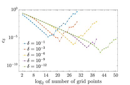
We first consider the non-preconditioned, direct application of the DMRG solver. We assemble the FE matrices in the QTT format and then solve the resulting system with the DMRG solver. Figure 1 displays the error $e_{\delta}$ obtained for varying values of $\delta$ and with $\varepsilon_{\mathrm{tol}}=10^{-10}$. We observe instabilities for all considered values of $\delta$. Choosing a different value of $\varepsilon_{\mathrm{tol}}$ did not influence the results.

We remark that we see three difference regions in the behavior of the error and that the first two regions correspond to the expected theoretical rates of convergence of the non compressed system, obtained in Proposition 5. Namely, denoting $h=1/(2^{L}+1)$,

• for $L\lesssim\left|\log_{2}\delta\right|$ (i.e., $h>\delta$), we observe convergence of order $\mathcal{O}(h^{1/2})$,

• for $L\gtrsim\left|\log_{2}\delta\right|$ (i.e., $h<\delta$), we observe convergence of order $\mathcal{O}(h)$,

while for large values of $L$ the approximation is unstable.

5.2. Preconditioned system

(a) $\varepsilon_{\mathrm{tol}}=10^{-8}$

(b) $\varepsilon_{\mathrm{tol}}=10^{-10}$

(c) $\varepsilon_{\mathrm{tol}}=10^{-10}$

Figure 2. Error $e_{\delta}$ as a function of the logarithm of the number of grid points for computations with preconditioner and $\delta\in\{10^{-1},10^{-3},10^{-6},10^{-9},10^{-12}\}$.

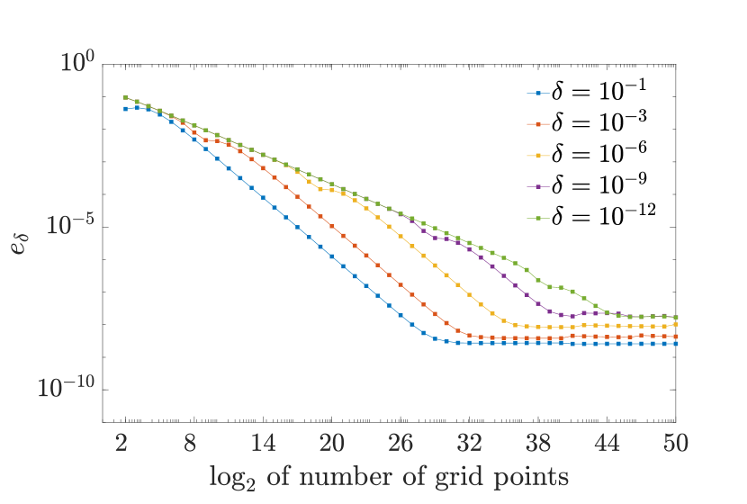
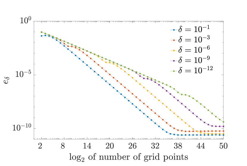
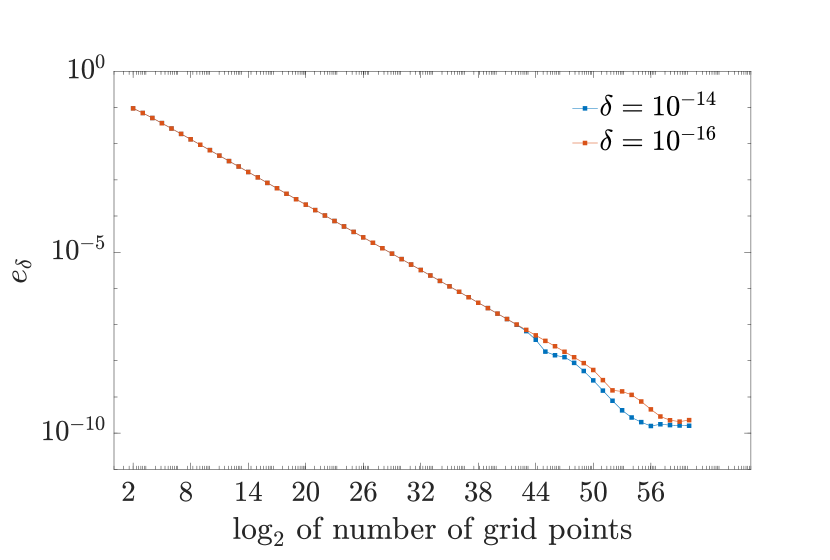
The numerical experiments in the previous section illustrate the need for preconditioning the QTT-compressed version of the algebraic equation (12) obtained from the $\mathbb{P}_{1}$-FE method. In this section we present the results from the simulations of the preconditioned and modified system, as described in Section 4. The simulations for varying values of $\delta$ and $\varepsilon_{\mathrm{tol}}$ are shown in Figure 2. We observe no instabilities, as were present in the non-preconditioned system. We also observe the same asymptotic rates observed for the stable region of the non-preconditioned solver and theoretically predicted in Proposition 5; in this case, though, for large values of $L$ the errors reach a plateau. The comparison of Figures 2(a) and 2(b) shows that this depends on the choice of $\varepsilon_{\mathrm{tol}}$.

Figure 3. Error $e_{\delta}$ as function of the number of degrees of freedom for computations with preconditioner, adaptive choice of $\varepsilon_{\mathrm{tol}}$, and for $\delta\in\{10^{-1},10^{-3},10^{-6},10^{-9}\}$.

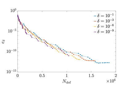
The error plot we have considered so far have all considered the variation of the error for a fixed truncation value $\varepsilon_{\mathrm{tol}}$. Estimate (20) of Theorem 1, though, gives a theoretical exponential rate of convergence, with constants independent of $\delta$. This can be realized, in practice, by choosing adaptively the truncation parameter $\varepsilon_{\mathrm{tol}}$, so that, for each $\delta$ and each $L$, the truncation error is of the same order of magnitude as the finite element error. Figure 3 displays the error $e_{\delta}$ as a function of the number of degrees of freedom for solutions obtained with the adaptive choice of the accuracy parameter $\varepsilon_{\mathrm{tol}}$ outlined. Specifically, for each $\delta$ and for each $L$, we choose the biggest $\varepsilon_{\mathrm{tol}}$ such that the error obtained is at most $10\%$ larger than the error $e_{\delta}$ obtained with $\varepsilon_{\mathrm{tol}}=10^{-12}$.

Figure 4. Error $e_{\delta}$ as a function of the cube root, left, and the square root, right, of the number of degrees of freedom for computations with preconditioner, adaptive choice of $\varepsilon_{\mathrm{tol}}$, and $\delta\in\{10^{-1},10^{-3},10^{-6},10^{-9}\}$.

Figure 5. Convergence rate coefficient estimation for $\delta\in\{10^{-1},10^{-3},10^{-6},10^{-9}\}$.

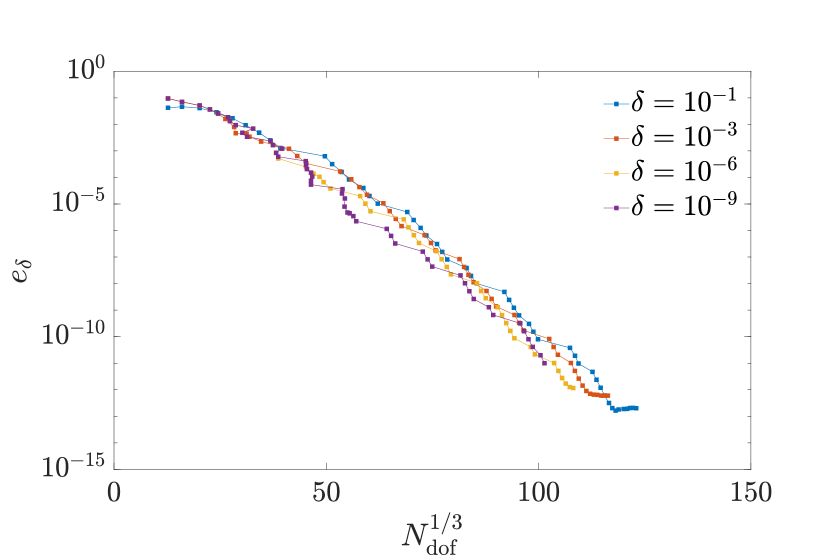
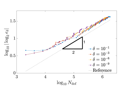
The same quantity is displayed in Figure 4, as a function of two different roots of the number of parameters of the QTT representation of the solution. It appears that the exponent $1/3$ in equation (20) of Theorem 1 constitutes, in this case, an underestimation of the rate of convergence. To properly study the experimental rate of convergence, we start from the ansatz that there exist $C,b,\kappa>0$ such that

(28) $$e_{\delta}=C2^{-b\left(N_{\mathrm{dof}}\right)^{\kappa}},$$

then, assuming that $\left|\log_{2}C\right|$ is small in comparison to $bN_{\mathrm{dof}}^{\kappa}$,

$$\left|\log_{2}e_{\delta}\right|=\left|\log_{2}C-b\left(N_{\mathrm{dof}}\right)^{\kappa}\right|\approx b\left(N_{\mathrm{dof}}\right)^{\kappa},$$

Hence

$$\log_{10}|\log_{2}e_{\delta}|\approx\log_{10}b+\kappa\log_{10}N_{\mathrm{dof}},$$

We plot then, in Figure 5, $\log_{10}\left|\log_{2}e_{\delta}\right|$ as a function of $\log_{10}N_{\mathrm{dof}}$, and estimate the exponent $\kappa$. In accordance with our previous observation, the values obtained strongly indicate that $\kappa=1/2$ for this set of computations.

6. Conclusions and future work

We have proved that the solutions of singularly perturbed PDEs in one dimension admit low rank QTT decompositions and that the energy norm of the error converges exponentially with respect to the third root of the number of parameters of the QTT decomposition, independently of the perturbation parameter. This is confirmed in a numerical test case, where we observe slightly better rates of convergence than prescribed by the theory, with errors independent of the perturbation parameter if an adaptive truncation strategy is chosen. Furthermore, the preconditioned system is stable at all perturbation scales and allows for the resolution of the boundary layer for very small perturbation parameters.

The natural extension of this work is the analysis of singularly perturbed problem in higher physical dimensions. This will be the subject of future investigation; we remark that our strategy to obtain rank bounds through high order approximation and $L^{2}$ projection extends rather naturally to this case.

Appendix A Assembly of preconditioner

We discuss here the details on the construction of the preconditioner. We follow the construction in [BK20], while introducing a modification to obtain stability independent of the perturbation parameter.

For all $0<\delta<1$, and for $f,c\in L^{2}(I)$, we introduce the singularly perturbed problem with homogeneous Dirichlet-Neumann boundary conditions of finding $v_{\delta}\in H^{1}(I)$ such that

(29) $$-\delta^{2}v_{\delta}^{\prime\prime}+cv_{\delta}=f, \text{ in }I,$$

$$v_{\delta}(0)=v_{\delta}^{\prime}(1)=0.$$

Let then $\widetilde{A}_{L}\in\mathbb{R}^{2^{L}\times 2^{L}}$ and $\widetilde{f}_{L}\in\mathbb{R}^{2^{L}}$ be, respectively, the matrix and the right hand side corresponding to the $\mathbb{P}_{1}$ FE discretization of (29) on the grid with nodes $\{j2^{-L}:j\in\{1,\dots,2^{L}\}\}$.

We introduce the following notation for the preconditioned system:

$$B_{L}\coloneqq C_{L}\widetilde{A}_{L}C_{L},\qquad g_{L}\coloneqq C_{L}\widetilde{f}_{L},$$

where the matrix $C_{L}$ has been introduced in (23). In order to solve the linear system $B_{L}\bar{u}_{L}=g_{L}$ in QTT format, we need to assemble $B_{L}$ and $g_{L}$. As shown in Section 2.3 and 2.4 in [BK20], there exist matrices $Q_{L,0},Q_{L,1},\Lambda_{L,0}$, and $\Lambda_{L,1}$ of small fixed QTT-rank such that

(30) $$B_{L}=Q_{L,0}^{T}\Lambda_{L,0}Q_{L,0}+Q_{L,1}^{T}\Lambda_{L,1}Q_{L,1}.$$

In what follows, we use normal parentheses $(\ )$ to indicate matrices and vectors and we use square brackets $[\ ]$ to indicate block structures with matrices or vectors as elements. Superscript $T$ on a matrix denotes the usual matrix transposition and superscript $T$ on a block structure (with elements being matrices or vectors) refers to transposition of the individual block elements.

A.1. Operations on TT-cores

We introduce some additional notation in order to present the explicit construction of the preconditioner. We represent TT-cores as block matrices and introduce two operations on TT-cores denoted by $\bullet$ and $\Join$. In Definition 1 we referred to $V^{1},\ldots,V^{d}\in\mathbb{R}^{r\times n\times r}$ as the TT-cores of $A$ with $r\in\mathbb{N}$ being the TT-rank of $A$ and $n\in\mathbb{N}$ the mode size of $A$. We generalize the definition mentioned above and introduce TT-cores of ranks $p\times q$ and mode sizes $m\times n$, for $p,q,m,n\in\mathbb{N}$.

Definition 6 ([BK20, Section 3.2]).

Let $m,n,p,q\in\mathbb{N}$ and let $U^{[\alpha,\beta]}\in\mathbb{R}^{m\times n}$ be tensors of sizes $m\times n$, for $\alpha=1,\ldots,p$ and for $\beta=1,\ldots,q$. We call the $4$-tensor $U\in\mathbb{R}^{p\times m\times n\times q}$ defined by

$$U(\alpha,i,j,\beta)=U^{[\alpha,\beta]}_{ij},$$

for all $\alpha=1,\ldots,p$, $i=1,\ldots,m$, $j=1,\ldots,n$ and $\beta=1,\ldots,q$, a TT-core of ranks $p\times q$ and of mode sizes $m\times n$. Given a $TT$-core $U$ of ranks $p\times q$ and of mode sizes $m\times n$, we call each tensor $U^{[\alpha,\beta]}$, $\alpha=1,\ldots,p$ and $\beta=1,\ldots,q$, the $(\alpha,\beta)$-block of $U$.

As a TT-core $U$ of ranks $p\times q$ and of mode sizes $m\times n$ is specified by the $2$-tensors $U^{[\alpha,\beta]}$, $\alpha=1,\ldots,p$ and $\beta=1,\ldots,q$, for ease of exposition and for convenience we can specify $U$ in the block structure

(31) $$U=\left[\begin{matrix}U^{[1,1]}&\cdots&U^{[1,q]}\\ \vdots&\ddots&\vdots\\ U^{[p,1]}&\cdots&U^{[p,q]}\end{matrix}\right].$$

We use the representation in equation (31) whenever we specify TT-cores. Then, by our convention for transposition, we have that

$$U^{T}(\alpha,i,j,\beta)=U(\alpha,j,i,\beta),$$

or equivalently,

$$(U^{T})^{[\alpha,\beta]}=(U^{[\alpha,\beta]})^{T}.$$

Definition 7 ([BK20, Section 3.2]).

Let $m,n,p,q\in\mathbb{N}$ and let $U$ be a TT-core of ranks $p\times q$ and of mode sizes $m\times n$. We define the $(i,j)$-slice $U^{\{i,j\}}\in\mathbb{R}^{p\times q}$ of $U$ as the matrix defined by

$$U^{\{i,j\}}_{\alpha,\beta}=U(\alpha,i,j,\beta).$$

In order to combine different TT-cores, we introduce two operations $\bullet$ and $\Join$ on TT-cores.

Definition 8 ([BK20, Definition 1]).

Let $p,q,r\in\mathbb{N}$ and let $m_{1},m_{2},n_{1},n_{2}\in\mathbb{N}$. Consider two TT-cores $U$ and $V$ of ranks $p\times r$ and $r\times q$ and of mode $m_{1}\times m_{2}$ and $n_{1}\times n_{2}$, respectively. The strong Kronecker product $U\Join V$ of $U$ and $V$ is the TT-core of rank $p\times q$ and mode size $m_{1}m_{2}\times n_{1}n_{2}$ given, in terms of matrix multiplication of slices of sizes $p\times r$ and $r\times q$, by

$$(U\Join V)^{\{i_{1}i_{2},j_{1}j_{2}\}}\coloneqq U^{\{i_{1},j_{1}\}}V^{\{i_{2},j_{2}\}}$$

for all combinations $i_{k}\in\{m_{1},\ldots,m_{k}\}$ and $j_{k}\in\{1,\ldots,n_{k}\}$ with $k=1,2$.

Definition 9 ([BK20, Definition 2]).

Let $p,p^{\prime},r,r^{\prime}\in\mathbb{N}$ and let $m,n,k\in\mathbb{N}$. Consider two TT-cores $A$ and $B$ of ranks $p\times p^{\prime}$ and $r\times r^{\prime}$ and of mode size $m\times k$ and $k\times n$, respectively. The mode core product $A\bullet B$ of $A$ and $B$ is the TT-core of rank $pr\times p^{\prime}r^{\prime}$ and mode size $m\times n$ given, in terms of matrix multiplication of blocks of size $m\times k$ and $k\times n$, by

$$(A\bullet B)^{\alpha\beta,\alpha^{\prime}\beta^{\prime}}\coloneqq A^{[\alpha,\alpha^{\prime}]}B^{[\beta,\beta^{\prime}]}$$

for all combinations of $\alpha=1,\ldots,p$, $\alpha^{\prime}=1,\ldots,p^{\prime}$, $\beta=1,\ldots,r$ and $\beta^{\prime}=1,\ldots,r^{\prime}$.

A.2. Construction of the preconditioner

We start by introducing some building block that will be necessary for the explicit TT-decompositions of the constituents of equation (30):

$$A_{b}\coloneqq A\bullet A,\ U_{b}\coloneqq U\bullet U^{T},\ X_{b}\coloneqq X\bullet X^{T},\ P_{b}\coloneqq P\bullet P,$$

where

$$U\coloneqq\left[\begin{matrix}I&J^{T}\\ &J\end{matrix}\right],\ X\coloneqq\frac{1}{2}\left[\begin{matrix}\Bigg{(}\begin{matrix}1\\ 2\end{matrix}\Bigg{)}&\Bigg{(}\begin{matrix}0\\ 1\end{matrix}\Bigg{)}\\ \Bigg{(}\begin{matrix}1\\ 0\end{matrix}\Bigg{)}&\Bigg{(}\begin{matrix}2\\ 1\end{matrix}\Bigg{)}\end{matrix}\right],\ P\coloneqq\left[\begin{matrix}1\\ 0\end{matrix}\right]$$

$$I\coloneqq\left(\begin{matrix}1&0\\ 0&1\end{matrix}\right),\ J=\left(\begin{matrix}0&1\\ 0&0\end{matrix}\right)$$

and for $\alpha\in\{0,1\}$

$$W_{\alpha}\coloneqq T_{\alpha}\bullet\bar{I},\ Z_{\alpha}\coloneqq Y_{\alpha}\bullet X^{T},\ K_{\alpha}\coloneqq N_{\alpha}\bullet P,$$

where

$$T_{1}\coloneqq\left[\begin{matrix}1\\ 1\end{matrix}\right],\ \bar{I}\coloneqq\left[\begin{matrix}1&0\\ 0&1\end{matrix}\right],\ Y_{0}\coloneqq\frac{1}{2}\left[\begin{matrix}\Bigg{(}\begin{matrix}1\\ 1\end{matrix}\Bigg{)}&\Bigg{(}\begin{matrix}0\\ 0\end{matrix}\Bigg{)}\\ \Bigg{(}\begin{matrix}-1\\ 1\end{matrix}\Bigg{)}&\Bigg{(}\begin{matrix}1\\ 1\end{matrix}\Bigg{)}\end{matrix}\right]$$

$$Y_{1}\coloneqq\frac{1}{2}\left[\Bigg{(}\begin{matrix}1\\ 1\end{matrix}\Bigg{)}\right],\ N_{1}\coloneqq[1],\ N_{0}\coloneqq\frac{1}{2}\left[\begin{matrix}\Bigg{(}\begin{matrix}1\\ 0\end{matrix}\Bigg{)}\\ \Bigg{(}\begin{matrix}0\\ 1\end{matrix}\Bigg{)}\end{matrix}\right].$$

Recall the different brackets $(\ )$ and $[\ ]$ and their respective meanings related to construction of TT-cores. We now state the TT-decompositions of the constituents of equation (30).

Lemma 7.

For any $L\in\mathbb{N}$, the matrix $C_{L}$ admits the TT-decomposition

(32) $$C_{L}=[\begin{matrix}A_{b}&\mu_{0,\delta}A_{b}\end{matrix}]\Join C_{1,L}\ldots\Join C_{L,L}\Join\left[\begin{matrix}\\ P_{b}\end{matrix}\right],$$

with TT-ranks equal to $8$ and where

(33) $$C_{\ell,L}=\left[\begin{matrix}U_{b}&\mu_{\ell,\delta}U_{b}\\ &2^{-1}X_{b}\end{matrix}\right],\qquad\text{for all }\ell=1,\ldots,L.$$

Proof.

Recall the definition of $C_{L}$

(34) $$C_{L}=\sum_{\ell=0}^{L}\mu_{\ell,\delta}P_{\ell,L}P^{T}_{\ell,L}.$$

By equation (86) in [BK20, Section 5.4], the following representation holds for every $\ell=0,\ldots,L$

$$2^{-\ell}P_{\ell,L}P^{T}_{\ell,L}=2^{-\ell}A_{b}\Join U_{b}^{\Join\ell}\Join(2^{-1}X_{b})^{\Join(L-\ell)}\Join P_{b}.$$

Thus, our modified expression is

(35) $$\mu_{\ell,\delta}P_{\ell,L}P^{T}_{\ell,L}=\mu_{\ell,\delta}A_{b}\Join U_{b}^{\Join\ell}\Join(2^{-1}X_{b})^{\Join(L-\ell)}\Join P_{b}$$

for $\ell=0,\ldots,L$. By inserting the expressions in equation (33) into equation (32), performing the multiplication and inserting the expression in equation (35), we end up with the expression for $C_{L}$ as given in equation (34). ∎

Lemma 8.

For any $L\in\mathbb{N}$ and for $\alpha\in\{0,1\}$, the matrix $Q_{L,\alpha}$ admits the TT-decomposition

(36) $$Q_{L,\alpha}=[\begin{matrix}A_{b}&\mu_{0,\delta}A_{b}\Join W_{\alpha}\end{matrix}]\Join Q_{1}\Join\ldots\Join Q_{L}\Join\left[\begin{matrix}\\ K_{\alpha}\end{matrix}\right]$$

with TT-ranks equal to $6$ and where

(37) $$Q_{\ell}=\left[\begin{matrix}2^{\frac{1}{2}}U_{b}&\mu_{\ell,\delta}2^{\alpha\ell+\frac{1}{2}}U_{b}\Join W_{\alpha}\\ &2^{\alpha-\frac{1}{2}}Z_{\alpha}\end{matrix}\right],\text{ for }\ell=1,\ldots,L.$$

Proof.

By equation (33c) in [BK20, Section 2.4], the following relation hold for $\alpha\in\{0,1\}$:

(38) $$Q_{L,\alpha}=M_{L,\alpha}C_{L}.$$

Moreover, by equation (88) in [BK20, Section 5.4] the following representation holds for every $\ell=0,\ldots,L$

$$2^{-\ell}M_{L,\alpha}P_{\ell,L}P^{T}_{\ell,L}=2^{-(1-\alpha)\ell}A_{b}\Join(2^{\frac{1}{2}}U_{b})^{\Join\ell}\Join W_{\alpha}\Join(2^{\alpha-\frac{1}{2}}Z_{\alpha})^{\Join(L-\ell)}\Join K_{\alpha}$$

Thus, our modified expression is

(39) $$\mu_{\ell,\delta}M_{L,\alpha}P_{\ell,L}P^{T}_{\ell,L}=\mu_{\ell,\delta}2^{\alpha\ell}A_{b}\Join(2^{\frac{1}{2}}U_{b})^{\Join\ell}\Join W_{\alpha}\Join(2^{\alpha-\frac{1}{2}}Z_{\alpha})^{\Join(L-\ell)}\Join K_{\alpha}$$

for $\alpha\in\{0,1\}$ and for $\ell=0,\ldots,L$. By inserting the expressions in equation (37) into equation (36), we end up with the same expression as when taking the sum over $\ell=0,\ldots,L$ of the expression in equation (39). The result now follows from the formula in equation (38) and equation (34):

$$Q_{L,\alpha}=M_{L,\alpha}C_{L}=\sum_{\ell=0}^{L}\mu_{\ell,\delta}M_{L,\alpha}P_{\ell,L}P_{\ell,L}^{T}.$$

∎

The explicit TT-decomposition of $\Lambda_{L,1}$ in equation (30) is presented below, while $\Lambda_{L,0}$ remains unchanged compared with [BK20].

Lemma 9.

For any $L\in\mathbb{N}$ the matrix $\Lambda_{L,1}$ admits the TT-decomposition

(40) $$\Lambda_{L,1}=\Lambda_{L,0}\Join\Lambda_{L,1,1}\Join\ldots\Join\Lambda_{L,L,1}\Join\Lambda_{L,L+1,1}$$

where $\Lambda_{L,\ell,1}=\frac{\delta^{2/L}}{2}I$, for $\ell=1,\ldots,L$, are TT-cores of ranks $1\times 1$ and of mode sizes $2\times 2$ and $\Lambda_{L,L+1,1}=1$ is a TT-core of ranks $1\times 1$ and of mode sizes $1\times 1$.

Proof.

By straightforward computation of the quantities in equations (90c) and (90c) in [BK20, Section 5.4] corresponding to the system matrix given by $S_{L}+R_{L}$ (instead of $\delta^{2}S_{L}+R_{L}$), we end up with equation (40) except that the intermediate TT-cores $\Lambda_{L,\ell,1}$, for $\ell=1,\ldots,L$, are given by $\frac{1}{2}I$ (instead of $\frac{\delta^{2/L}}{2}I$). Lemma 7 and Lemma 8 do not include the factor of $\delta^{2}$ in the system matrix $\delta^{2}S_{L}+R_{L}$. Clearly,

$$(\delta^{2/L})^{L}=\delta^{2},$$

and thus we obtain the decomposition for $\Lambda_{L,\alpha}$ of the system matrix $\delta^{2}S_{L}+R_{L}$ by multiplying the obtained expression for $\Lambda_{L,\ell,1}$, $\ell=1,\ldots,L$, with $\delta^{2/L}$. This yields the desired decomposition as given in equation (40). ∎

Lemmas 7, 8, and 9 provide a complete explicit TT-representation of the preconditioned system matrix $B_{L}$ in equation (30).

A.3. Application of preconditioner

The preconditioner in the previous subsection was introduced for Dirichlet-Neumann boundary value problems with homogeneous boundary conditions. We show here how to apply it to the Dirichlet-Dirichlet case numerically approximated in Section 5. We suppose then, for ease of exposition, that the reaction coefficient is constant $c(x)\equiv\overline{c}\in\mathbb{R}$ for all $x\in I$. The first step is to instead consider the following problem with homogeneous boundary conditions

(41) $$-\delta^{2}v_{\delta}^{\prime\prime}+cv_{\delta} =f-cg,\text{ in }(0,1)$$

$$v_{\delta}(0)=0,\ v_{\delta}(1) =0,$$

where $g(x)\coloneqq\alpha_{1}x-\alpha_{0}(x-1)$, whose solution relates to the solution of (LABEL:DiffEq) as $v_{\delta}(x)=u_{\delta}(x)-g(x)$. We also introduce the corresponding Dirichlet-Neumann problem

(42) $$-\delta^{2}v_{\delta}^{\prime\prime}+cv_{\delta} =f-cg,\text{ in }(0,1)$$

$$v_{\delta}(0)=0,\ v_{\delta}^{\prime}(1) =0,$$

for which we have introduced the preconditioner $C_{L}$ (23).

We use the well-known Sherman-Morrison formula [Hag89] to transfer the solution of the preconditioned discretization of (42) to the case with Dirichlet-Dirichlet boundary conditions as in (41).

Theorem 2 ([EM06]).

Let $B\in\mathbb{R}^{n\times n}$ be an invertible matrix and let $u,v\in\mathbb{R}^{n}$ be such that also $B+uv^{T}$ is invertible. Then the inverse of $B+uv^{T}$ is given by

(43) $$(B+uv^{T})^{-1}=B^{-1}-\frac{B^{-1}uv^{T}B^{-1}}{1+v^{T}B^{-1}u}$$

The following straightforward corollary suggests how to apply, in practice, the Sherman-Morrison formula for solving linear systems.

Corollary 3 ([EM06, Corollary 2]).

Let $B\in\mathbb{R}^{n\times n}$ and let $u,v,y\in\mathbb{R}^{n}$. Suppose that $B$ and $B+uv^{T}$ are invertible matrices and suppose that $x_{1}\in\mathbb{R}^{n}$ satisfies $Bx_{1}=y$ and that $x_{2}\in\mathbb{R}^{n}$ satisfies $Bx_{2}=u$. Then

(44) $$x_{3}\coloneqq x_{1}-\frac{v^{T}x_{1}}{1+v^{T}x_{2}}x_{2}$$

satisfies $(B+uv^{T})x_{3}=y$.

We may express $A_{L}$, in terms of a rescaling of the parts of $\widetilde{A}_{L}$ (since the Dirichlet-Dirichlet and Dirichlet-Neumann cases have different mesh sizes) and of a rank-one correction term. Therefore, the solution of the singularly perturbed problem with homogeneous Dirichlet boundary conditions can be obtained using Corollary 3. In the case where $c$ is nonconstant, then the preconditioned solution for the Dirichlet-Dirichlet case can be obtained in a similar fashion, provided that the integrals arising in $\Lambda_{L,0}$ are computed using the grid $\mathcal{T}^{\mathrm{int}}_{L}$.

References

- [BK20] M. Bachmayr and V. Kazeev, Stability of low-rank tensor representations and structured multilevel preconditioning for elliptic PDEs, Found. Comput. Math. (2020).
- [BL76] J. Bergh and J. Löfström, Interpolation spaces - an introduction, Springer-Verlag Berlin Heidelberg 1976, 1976.
- [BPV00] J. Bramble, J. Pasciak, and P. Vassilevski, Computational scales of Sobolev norms with application to preconditioning, Math. Comput. 69 (2000), no. 230, 463–480.
- [BPX90] J. H. Bramble, J. E. Pasciak, and J. Xu, Parallel multilevel preconditioners, Math. Comput. 55 (1990), no. 191, 1–22.
- [BS08] S. C. Brenner and L. R. Scott, The mathematical theory of finite element methods, third ed., Texts in Applied Mathematics, vol. 15, Springer, New York, 2008.
- [CHT20] M. D. Chekroun, Y. Hong, and R. M. Temam, Enriched numerical scheme for singularly perturbed barotropic quasi-geostrophic equations, J. Comput. Phys. 416 (2020), 109493, 28.
- [COR16] A. V. Chertkov, I. Oseledets, and M. Rakhuba, Robust discretization in quantized tensor train format for elliptic problems in two dimensions, arXiv:1612.01166, 2016.
- [DS14] S. V. Dolgov and D. V. Savostyanov, Alternating minimal energy methods for linear systems in higher dimensions, SIAM J. Sci. Comput. 36 (2014), no. 5, A2248–A2271.
- [EG04] A. Ern and J. Guermond, Theory and practice of finite elements, Applied Mathematical Sciences, vol. 159, Springer-Verlag, New York, 2004.
- [EM06] N. Egidi and P. Maponi, A Sherman-Morrison approach to the solution of linear systems, J. Comput. Appl. Math. 189 (2006), no. 1-2, 703–718.
- [Hag89] W. W. Hager, Updating the inverse of a matrix, SIAM Rev. 31 (1989), no. 2, 221–239.
- [Hit27] F. Hitchcock, The expression of a tensor or a polyadic as a sum of products, Journal of Mathematics and Physics 6 (1927), 164–189.
- [KB09] T. G. Kolda and B. W. Bader, Tensor decompositions and applications, SIAM Rev. 51 (2009), no. 3, 455–500.
- [Kho11] B. N. Khoromskij, O(d log n)-quantics approximation of n-d tensors in high-dimensional numerical modeling, Constr. Approx. 34 (2011), 257–280.
- [Kho18] by same author, Tensor numerical metods in scientific computing, De Gruyter, Berlin/Munich/Boston, 2018.
- [KK12] V. Kazeev and B. N. Khoromskij, Low-rank explicit QTT representation of the Laplace operator and its inverse, SIAM J. Matrix Anal. Appl. 33 (2012), no. 3, 742–758.
- [KS15] V. Kazeev and C. Schwab, Tensor approximation of stationary distributions of chemical reaction networks, SIAM J. Matrix Anal. Appl. 36 (2015), no. 3, 1221–1247.
- [KS18] by same author, Quantized tensor-structured finite elements for second-order elliptic PDEs in two dimensions, Numer. Math. 138 (2018), no. 1, 133–190.
- [Lio73] J.-L. Lions, Perturbations singulières dans les problèmes aux limites et en contrôle optimal, Lecture Notes in Mathematics, Vol. 323, Springer-Verlag, Berlin-New York, 1973.
- [Mel02] J. Melenk, hp-finite element methods for singular perturbations, Springer-Verlag Berlin Heidelberg, 2002.
- [MRS19] C. Marcati, M. Rakhuba, and C. Schwab, Tensor rank bounds for point singularities in , Tech. Report 2019-68, Seminar for Applied Mathematics, ETH Zürich, Switzerland, 2019.
- [MX16] J. M. Melenk and C. Xenophontos, Robust exponential convergence of -FEM in balanced norms for singularly perturbed reaction-diffusion equations, Calcolo 53 (2016), no. 1, 105–132.
- [Ose10] I. Oseledets, Approximation of matrices using tensor decomposition, SIAM J. Matrix Anal. Appl. 31 (2010), no. 4, 2130–2145.
- [Ose11a] by same author, Tensor-train decomposition, SIAM J. Sci. Comput. 33 (2011), 2295–2317.
- [Ose11b] by same author, Tensor-train ranks for matrices and their inverses, Comput. Meth. Appl. Math. 11 (2011), no. 3, 394–403.
- [Ose13] by same author, Constructive representation of functions in low-rank tensor formats, Constr. Approx. 37 (2013), 1–18.
- [OT10] I. Oseledets and E. Tyrtyshnikov, Tt-cross approximation for multidimensional arrays, Linear Algebra Appl. 432 (2010), no. 1, 70–88.
- [Rak19] M. Rakhuba, Robust solver in a quantized tensor format for three-dimensional elliptic problems, Tech. Report 2019-30, ETH Zürich, Switzerland, 2019.
- [Sch98] C. Schwab, p- and hp- finite element methods - theory and applications in solid and fluid mechanics, Oxford Univ. Press, 1998.
- [Sch11] U. Schollwöck, The density-matrix renormalization group in the age of matrix product states, Ann. Physics 326 (2011), no. 1, 96–192.
- [SS96] C. Schwab and M. Suri, The p and hp version of the finite element method for problems with boundary layers, Math. Comp. 65 (1996), no. 216, 1403–1429.
- [SW83] A. Schatz and L. Wahlbin, On the finite element method for singularly perturbed reaction-diffusion problems in two and one dimensions, Math. Comp. 40 (1983), no. 161, 47–89.
- [Whi92] S. R. White, Density matrix formulation for quantum renormalization groups, Phys. Rev. Lett. 69 (1992), 2863–2866.