Black Hole Mass Accretion Rates and Efficiency Factors for over 750 AGN and Multiple GBH
Abstract
Mass accretion rates in dimensionless and physical units, and efficiency factors describing the total radiant luminosity of the disk and the beam power of the outflow are studied here. Four samples of sources including 576 LINERs, 100 classical double (FRII) radio sources, 80 relatively local AGN, and 103 measurements of four stellar mass X-ray binary systems, referred to as Galactic Black Holes (GBH), are included in the study. All of the sources have highly collimated outflows leading to compact radio emission or powerful extended (FRII) radio emission. The properties of each of the full samples are explored, as are those of the four individual GBH, and sub-types of the FRII and local AGN samples. Source types and sub-types that have high, medium, and low values of accretion rates and efficiency factors are identified and studied. A new efficiency factor that describes the relative impact of black hole spin and mass accretion rate on the beam power is defined and studied, and is found to provide a new and interesting diagnostic. Mass accretion rates for 13 sources and efficiency factors for 6 sources are compared with values obtained independently, and indicate that similar values are obtained with independent methods. The mass accretion rates and efficiency factors obtained here substantially increase the number of values available, and improve our understanding of their relationship to source types. The redshift dependence of quantities is presented and the impact on the results is discussed.
keywords:
black hole physics – galaxies: activeAccepted XXX. Received YYY; in original form ZZZ
1 Introduction
Mass accretion rates and associated efficiency factors are important quantities that describes the state of stellar and supermassive black hole systems. They provide information regarding processes that lead to the accretion, the state of the accretion disk, and how outflows and winds from accreting systems can affect their environment. Thus, they are important diagnostics of the state of the black hole system (e.g. Heckman & Best 2014; Yuan & Narayan 2014). Accretion rates and efficiency factors have been determined using a variety of methods and diagnostics, and this has allowed estimates of these quantities for sources with a broad range of properties (e.g. Bian & Zhao 2003; Davis & Laor 2011; Raimundo et al. 2012; Wu, Lu, & Zhang 2013; Trakhtenbrot 2014; Netzer & Trakhtenbrot 2014; Trakhtenbrot, Volonteri, & Natarajan 2017; Jiang et al. 2019; O’Dea & Saikia 2020).
Here, the new method of obtaining mass accretion rates introduced by Daly (2019) is applied to obtain and study accretion rates and efficiency factors. The "outflow method," developed and applied by Daly (2016, 2019) (hereafter D16 and D19) and Daly et al. (2018), (hereafter D18) applies to black hole systems that include a black hole, accretion disk, and a highly collimated outflow. The highly collimated outflow must lead to radio emission from a compact radio source or from a powerful extended radio source that can be used to study the properties of the highly collimated outflow, as described in section 2. The method allows empirical determinations of accretion disk properties such as the mass accretion rate and disk magnetic field strength in dimensionless and physical units.
1.1 Overview of the Outflow Method
The outflow method of determining and studying black hole spin and accretion disk properties was proposed and applied by D16 and D19, and followed the methods developed and applied by Daly (2009, 2011) and Daly & Sprinkle (2014) to estimate black hole spin values based on outflow beam powers. A detailed overview of the method, it’s development, and it’s application is provided in section 1.1 of D19. The method is empirically based, and includes one key theoretical input, as described below. To understand the method and it’s application it is important to relinquish preconceived notions and assumptions that are based on the application of specific accretion disk or other models and focus on what is indicated empirically.
As is often the case with theoretical developments, with hindsight, simple arguments that are consistent with the original method become evident, even though this is not the way the method was developed or the results obtained. In this spirit, a heuristic path to understand the method and its application is described here. This provides an alternative path to arrive at the same conclusions even though this is not the way the equations were derived, which is explained in detail in section 1.1. of D19.
Consider a black hole with irreducible mass and dimensionless spin parameter that has an accretion disk accreting matter at a rate in solar masses per year. A priori, these three quantities are independent. Given that the accretion disk of the system produces some bolometric luminosity, , the radiant efficiency of the disk may be determined empirically when is known.
The outflow method has one key theoretical input, and the introduction of this theoretical input is motivated empirically. It is motivated by the fact that there are numerous black hole systems with outflow beam powers that exceed the bolometric luminosity of the disk by one to two orders of magnitude. For example, the results of D18 indicate that there are numerous black hole systems with beam powers that are 10 - 100 times larger than the bolometric luminosity of the accretion disk of the system (see Fig. 2 of D18). In these cases, it is reasonable to suppose that the highly collimated outflow is powered at least in part by the black hole spin (see also Narayan & McClintock 2012, and Daly 2011). D18 also showed that the slopes and normalizations of the relationship between and are consistent within uncertainties for the four samples studied, even though these quantities have a broad range of values of about to for and to for , where is the beam power and is the Eddington luminosity. This suggests that the sources in the four samples studied by Daly et al. (2018) are governed by the same physics, and therefore, all of the outflows are powered at least in part by black hole spin.
This indicates that the functional form of the theoretical equation that describes spin powered outflows (e.g. Blandford & Znajek 1977; Blandford 1990; Meier 1999) may be compared with the functional form of empirically determined relationships (D16, D18, D19). Once the theoretical equation is written in dimensionless separable form (see eq. 1), terms in the empirically determined relationship may be identified with terms in the theoretical equation to solve for the properties of the accretion disk and black hole spin. Eq. (1) is the primary theoretical input to the outflow method. Other aspects of the method are empirically based. No particular accretion disk emission model is assumed, and no detailed jet power/emission model is adopted.
D19 showed that the fundamental equation that describes outflows that are powered at least in part by black hole spin, (e.g. Blandford & Znajek 1977; Blandford 1990; Meier 1999) is separable and may be written as
| (1) |
(see eq. 6 from D19). Here is the beam power of the outflow, or the energy per unit time carried away from the black hole region in the form of a collimated outflow, typically thought to be in the form of directed kinetic energy, is the poloidal component of the accretion disk magnetic field, is the disk magnetic field strength, is the Eddington magnetic field strength (e.g. Rees 1984; Blandford 1990; Dermer, Finke, & Menon 2008), , is the total black hole mass, the normalized spin function is where is the spin function and is the maximum value of this function (see D19), is the normalization factor for the beam power in units of the Eddington Luminosity, , . It is clear that this is separable: information regarding the outflow is described by and ; that related to black hole spin is described by ; and, as explained below, that related the accretion event is described by the term (see eq. 7 of D19), where the value of is obtained for each sample from Table 2 of D18, as summarized by D19, and is typically . Note that the ratio is absorbed into the normalization factor . The method was further developed and applied by D19 to study black hole spin functions and spin, the magnetic field strength of the accretion disk, in physical units, and the magnetic field strength or pressure of the accretion disk in the dimensionless form . This work did not explicitly compute mass accretion rates in physical units or efficiency factors. These topics are addressed in this paper.
The identification of terms in eq. (1) with empirically determined quantities was carried out with detailed calculations, presented and discussed by D16, D18, and D19. With hindsight a simple identification of terms becomes evident. The empirically determined relationship between beam power and disk luminosity, which by construction does not include a term related to black hole spin, has the form where the only term related to the overall properties of the accretion disk is . In the theoretical equation given by eq. (1) there is only one term that describes the overall properties of the accretion disk, and that is the term . Thus, identifying these terms, and noting that each is normalized to have a maximum value of unity, it is easy to see that
| (2) |
as originally indicated by the detailed calculations discussed by D19.
To see how this is related to mass accretion rate, consider standard representations (e.g. Yuan & Narajan 2014; Ho 2009) for the bolometric disk luminosity
| (3) |
and the beam power
| (4) |
where the efficiency factor that describes the radiant luminosity of the disk is not assumed to be constant, the dimensionless mass accretion rate is defined as , and the Eddington mass accretion rate is defined as . (Some authors adopt different definitions of the Eddington mass accretion rate and the dimensionless mass accretion rate. It is shown in section 3.3 that consistent results are obtained with those definitions and the definitions adopted here.) Though eq. (4) is most frequently adopted for sources with low values of , it is reasonable to suppose that the same relationship holds for all of the sources since the samples studied include many sources with low values of , and all of the samples have consistent values of the slope and normalization relating to (e.g. D18). Combining eqs. (1), (2), (3), and (4), we obtain
| (5) |
where the constant of proportionality must be unity because and are each normalized to have a maximum value of one. Thus, or for and , respectively (see also Ho 2009). Note that in D16, a more general functional form for was adopted, and the same results were obtained. For the types of sources studied here, is only a constant when , which is quite clearly ruled out for these sources (D16, D18, D19). Substituting eq. (3) into eq. (2), and applying eq. (5), we obtain
| (6) |
Thus,
| (7) |
so can be empirically determined using eq. (7).
It is interesting to note that empirical results indicate and thus are independent of the black hole spin function and black hole spin (D16, D19). This is also suggested by the fact that there is no empirical indication that the relationship between and changes as , for the sources studied, as discussed by D16 and D19.
It is interesting to note that eq. (2) provides an estimate of the gas pressure of the accretion disk in dimensionless form (see section 3.3. of D19). And the magnetic field strength of the disk, which is obtained from eq. (2), provides an estimate of the disk pressure in physical units (see section 3.1 of D19).
Here, four samples of sources, including 756 AGN and 103 measurements of four stellar-mass black holes associated with X-ray binaries are considered. The samples, source parameters, and parameter uncertainties are described in section 2. Methods of obtaining mass accretion rates and efficiency factors are described in sections 3.1 and 3.2, respectively. The results are discussed in section 4.1 and 4.2, respectively. An overview of the different source parameters associated with the accretion disk that can be obtained with the method, and the impact of the redshift range of the sources on the results are discussed in section 5. The conclusions are summarized in section 6.
2 Data
Four samples are considered here. The samples include 576 LINERs from Nisbet & Best (2016) (hereafter NB16); 100 classical double (FRII) sources from D16 and D19; 80 local AGN that are compact radio sources from Merloni et al. (2003) (hereafter M03); and 103 observations of four stellar-mass Galactic Black Hole systems (GBH) that are in X-ray binary systems. The stellar-mass GBH data includes the 102 observations listed in Table 2 of D19 plus one observation of A0 6200 discussed in section 5 of D19 (the data for the second observation of A0 6200 is from Gou et al. 2010; Kuulkers et al. 1999; and Owen et al. 1976). These are stellar mass X-ray binaries, and each of the GBH have multiple simultaneous radio and X-ray observations (Saikia et al. 2015) (hereafter S15) who obtained the data from Corbel et al. (2013), Corbel, Körding, & Kaaret (2008), Zycki, Done & Smith (1999), Shahbaz et al. (1996), Merloni et al. (2003), Gallo et al. (2006), Gelino, Harrison & Orosz (2001), Shahbaz, Naylor & Charles (1994), and Jonker & Nelemans (2004). These four samples were studied by D19 who reported spin functions, spin values, and accretion disk magnetic field strengths in dimensionless and physical units for each source and observation.
The samples were selected for the purpose of studying black hole spin using source outflow properties following the work of Daly (2009, 2011), Narayan & McClintock (2012), and Daly & Sprinkle (2014), for example. It has long been thought that powerful collimated outflows from black hole systems are likely to be powered by black hole spin (e.g. Blandford & Znajek 1977; Rees 1984; Begelman, Blandford, & Rees 1984; Blandford 1990).
Individual samples, each comprised of a specific type of source including the NB16 LINERs, D16/D19 FRII (classical double) sources, M03 local AGN sample, and the S15 stellar-mass GBH were selected. The four different types of black hole systems allow studies of and comparisons between four different categories of black hole system, including supermassive and stellar-mass systems. Another criteria was that reliable determinations of the bolometric disk luminosity, beam power, and black hole mass were available.
The NB16 LINERS, M03 AGN, and S15 GBH all lie on the fundamental plane of black hole activity. Thus, black hole masses were available for all of the sources, bolometric disk luminosities were obtained from the (2 - 10) keV X-ray luminosity using a standard conversion (e.g. Ho 2009; D18), and the beam powers were obtained by rotating the fundamental plane to the fundamental line of black hole activity using eq. (4) of D18 and the values of C and D listed in Table 1 of D18 for each sample. Note that time variability of the mass accretion rate and it’s impact on various source properties is discussed in detail in sections 5 and 6 of D19. For the FRII sources, the black hole masses were obtained from McLure et al. (2004, 2006). The bolometric disk luminosities were obtained from the O[III] luminosities of Grimes, Rawlings & Willott (2004) using a standard conversion (e.g. Heckman et al. 2004; Dicken et al. 2014). The beam powers were obtained using the strong shock method (described in detail in section 1.1 of D19) for 12 of the sources (O’Dea et al. 2009), and the relationship between beam power and 178 MHz radio luminosity obtained by Daly et al. (2012) using 31 sources with beam powers determined with the strong shock method (O’Dea et al. 2009). The source types are from Grimes, Rawlings & Willott (2004); W sources have weak emission lines, and Q sources are quasars.
Uncertainties of all quantities used to determine the black hole mass, bolometric luminosity, and beam power were included to obtain the uncertainty of each of these quantities, as described in section 2 of D19. The uncertainties , , listed in section 2 of D19 are propagated to obtain uncertainties of all the quantities discussed in this paper using a method identical to that described in detail in section 3.3 of D19. For the GBH, the uncertainty of the black hole mass is small compared with uncertainties of the bolometric disk luminosity and the beam power, so uncertainties of the black hole mass are neglected for the GBH. In addition, the black hole mass of a given GBH is constant during the outflow events, and the black hole mass range for the GBH is small, so neither the dispersion of the GBH black hole mass nor the uncertainty of GBH black hole masses are included in Table 1.
Here, the dimensionless disk magnetic field strength, that is, the ratio of the accretion disk field strength to the Eddington magnetic field strength, is used to obtain the mass accretion rate in dimensionless and physical units for each system and for each observation of the GBH. The mass accretion rate of each source is combined with the bolometric disk luminosity, outflow beam power, and black hole spin function to define and study three efficiency factors associated with each black hole system, and the properties of different samples and types of sources are summarized in Table 1. Mass accretion rates and bolometric efficiency factors obtained here are compared with those obtained independently in Table 2. Results for individual sources and observations are listed in Tables 3 - 6, and provide a measure of the state of the system at the time of the observation, since any given source may be time variable. Quantities are obtained in the context of a spatially flat cosmological model with mean mass density of non-relativistic matter relative to the critical density today of , a similarly normalized cosmological constant of , and a value of Hubble’s constant of 70 km/s/Mpc.
3 Method
3.1 The Mass Accretion Rate in Dimensionless and Physical Units
The mass accretion rate of each source in dimensionless and physical units can be empirically determined using the results obtained by D19 who showed that the dimensionless mass accretion rate , where B is the strength of the magnetic field anchored in the accretion disk and is the Eddington magnetic field strength (e.g. Rees 1984); D19 list empirically determined values of and for each source. Given the definition of the dimensionless mass accretion rate, , it is easy to see that
| (8) |
where is the Eddington luminosity of the hole, , so the mass accretion rate in physical units can be obtained from . The results are summarized in Table 1.
A comparison between mass accretion rates obtained here with those obtained independently are discussed in section 4.1 and are shown in Table 2.
Table 1 includes the mean value and dispersion of each quantity, with the dispersion measured by the one sigma standard deviation of the sample or sub-sample. The uncertainty per source of each quantity is included in (brackets) following the mean value and dispersion of each quantity in the top part of Table 1. The uncertainty per source of each quantity is obtained by propagating the uncertainties , , of the input parameters adopting a value of for all samples, as described in section 2.
3.2 Accretion Disk and Outflow Efficiency Factors
The efficiency factor of the accretion disk, , is defined as
| (9) |
For the sources studied here, is determined from the [OIII] for the FRII sources, and from the (2-10) keV X-ray luminosity for the other samples (see D16 and D18), and the values of listed in Tables 2-5 from D19 are applied here. The mass accretion rate is obtained as described in sections 1.1 and 3.1.
A comparison between bolometric efficiency factor values, , obtained here with those obtained independently are discussed in section 4.2 and are shown in Table 2.
The efficiency factor of the outflow, , is defined as
| (10) |
Outflow beam powers are based on the strong shock method for the FRII sources and on the mapping from the fundamental plane of black hole activity to the fundamental line of black hole activity for the three other samples, as described by D18 and D19 (see also O’Dea et al. 2009). The values of listed in Tables 2-5 from D19 are applied here.
A new efficiency factor that measures the relative impact of black hole spin and the accretion disk on the Eddington-normalized beam power, , is referred to as the "spin relative to disk" efficiency factor. This efficiency factor is
| (11) |
This ratio is interesting because beam power in Eddington units may be written as, , so the ratio measures the relative impact of black hole spin and the dimensionless mass accretion rate on the Eddington normalized outflow beam power (see eq. 4).
The sample or sub-sample mean value and dispersion is listed in Table 1 for each quantity, and the uncertainty per source is included in brackets in top part of Table 1, as described in section 2 and 3.1.
3.3 Comparison with other Representations of Key Equations
Throughout these investigations, the total radiant luminosity of the accretion disk is represented in the standard form , where the efficiency factor is not assumed to be constant (see section 1.1). The dimensionless mass accretion rate and Eddington mass accretion rate are defined to be and , respectively.
An equivalent representation can be obtained by absorbing the efficiency factor into the definition of the Eddington mass accretion rate (e.g. Yuan & Narayan 2014). If the Eddington mass accretion rate is defined as , and the dimensionless mass accretion rate is defined as , then becomes , with .
Since both D16 and D19 empirically determined that the efficiency factor can not be constant for the sources studied, the first representation given by eq. (3), which allows explicit tracking of this efficiency factor, was selected.
4 Results
Mass accretion rates in dimensionless and physical units obtained as described in section 3.1 and efficiency factors obtained as described in section 3.2 are summarized in Table 1. The mean value and dispersion (i.e. the one sigma standard deviation) for the sample, sub-sample, or source listed in column (1) are provided for each quantity. The estimated uncertainty per source of each quantity is indicated in brackets following the mean value and dispersion in the top part of the table, obtained as described in section 2 and 3.1. The input values used to compute each quantity are obtained from D19; for completeness, black hole mass is included in the Tables presented here.
A comparison of mass accretion rates and bolometric efficiency factors obtained independently is provided in Table 2.
Mass accretion rates, efficiency factors, and black hole masses for each source and measurement for the S15 sample of GBH, the D16/D19 sample of classical double (FRII) sources, the M03 sample of local AGN, and the NB16 sample of LINERs are listed in Tables 3, 4, 5, and 6, respectively.
4.1 Mass Accretion Rates
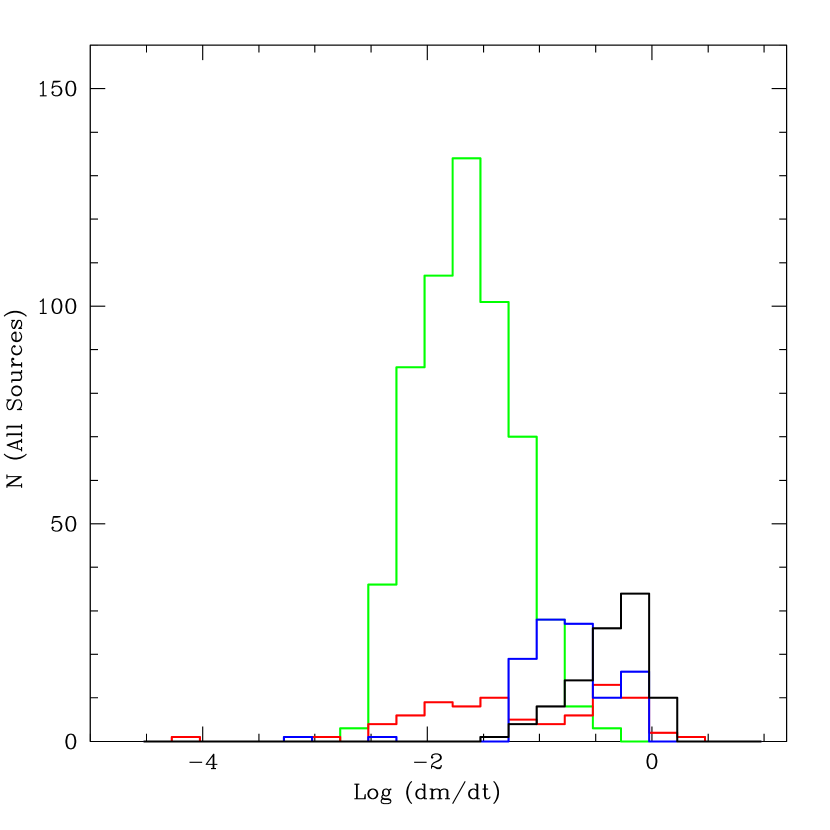
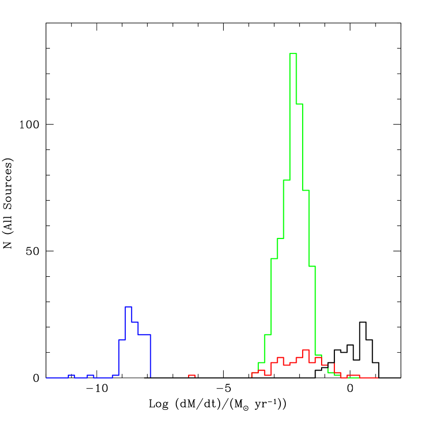
Histograms of mass accretion rates in dimensionless and physical units are shown in Figs. 1 - 2. The mean value and one sigma dispersion of each sample is listed in the first part of Table 1. The sample is indicated in column (1), the source type is indicated in column (2), the number of sources (or number of measurements for GBH) included in the mean and dispersion is listed in column (3), mean values for the mass accretion rate in dimensionless and physical units are listed in columns (4) and (5), respectively.
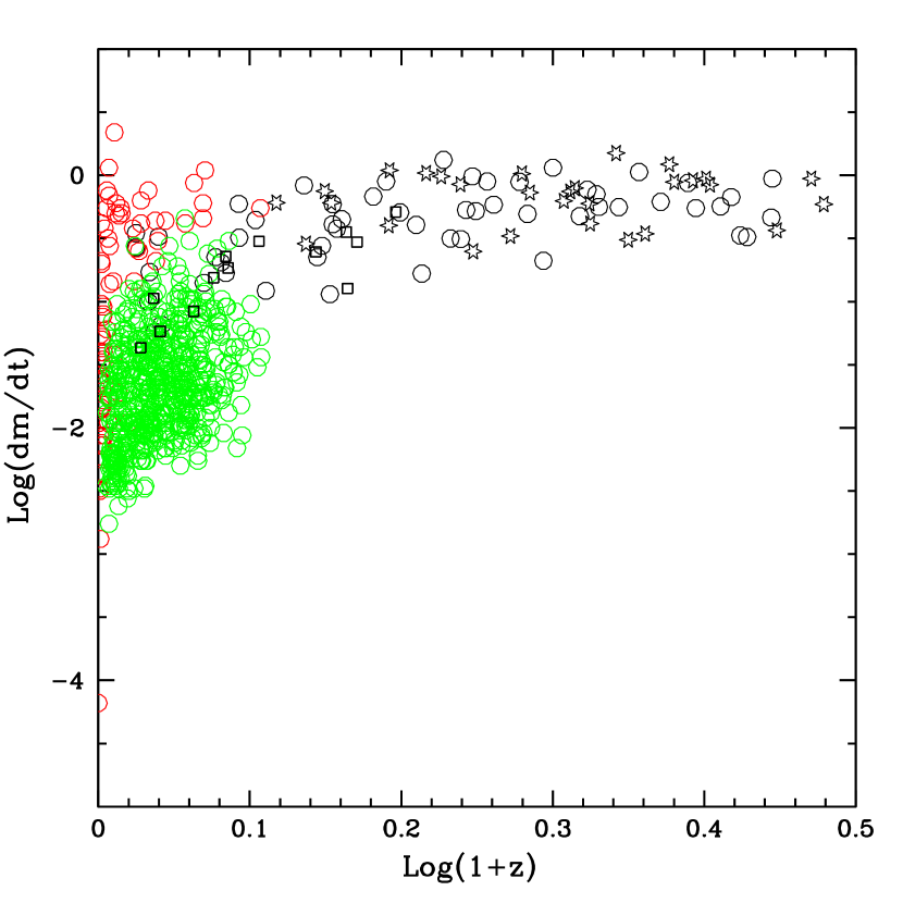
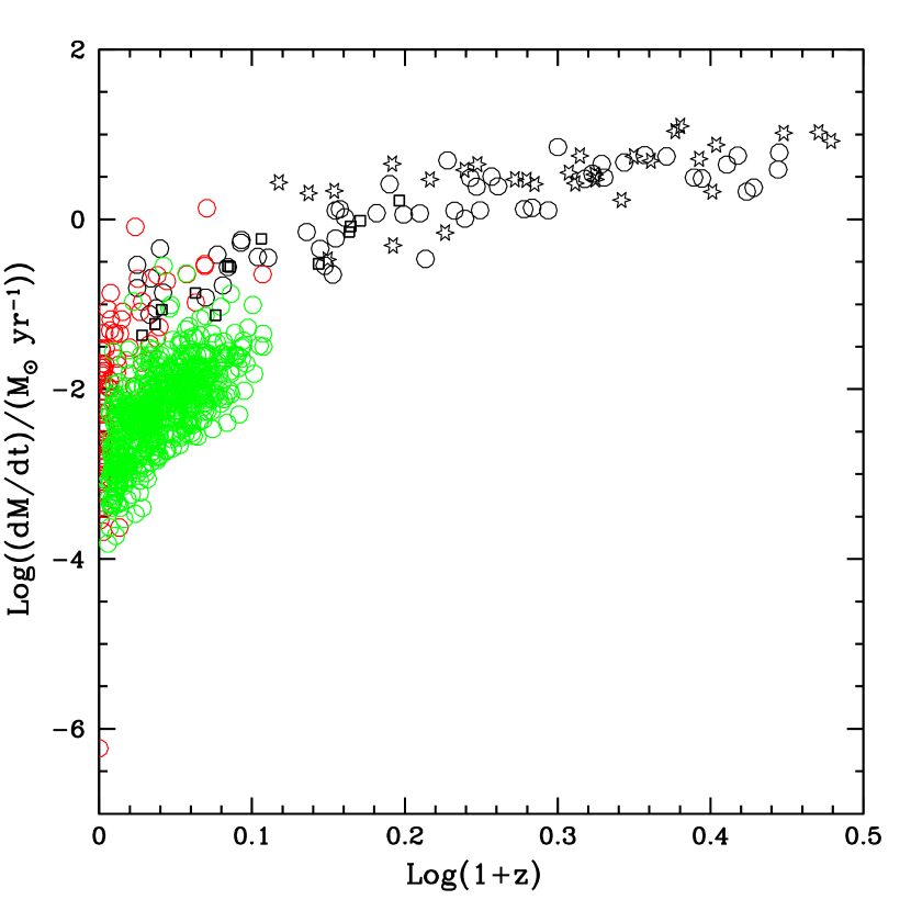
For AGN the dimensionless mass accretion rates are related to AGN type, as is evident from the values listed in the first four lines of Table 1, as expected based on the study by Ho (2009). The 100 FRII sources have the highest mass accretion rates for rates expressed in both dimensionless and physical units. Part of the reason for this is that the sample includes sources with redshifts between about zero and two, as illustrated in Figs. 3 - 4, and the mass accretion rate in physical units increases with redshift. The M03 sample of local AGN has the second highest mass accretion rate, though there is substantial overlap between the M03 and NB16 samples for the mass accretion rate in physical units, and between the M03 sample and both the D19 and NB16 samples for the rate in dimensionless units. The mean dimensionless mass accretion rate for the GBH is similar to that for the AGN and, of course, the rate in physical units is much smaller than that obtained for AGN. The maximum values of the dimensionless mass accretion rate are close to unity, indicating that all of the sources studied here are accreting at Eddington or sub-Eddington levels. This limit is not externally imposed.
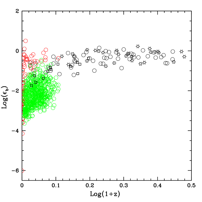
It is clear from Figs. 3 - 4 that sources with lower values of and , which are evident at low redshift, drop out of each sample as redshift increases. This effect is particularly striking for and is likely a selection effect whereby sources with lower bolometric disk luminosities or lower radio luminosities that are at larger distances and redshift require observations to lower flux densities to be detected, and thus in flux limited surveys these sources drop out of the sample as redshift increases. Thus, the different distributions of seen in Fig. 4 is affected by these redshift selection effects. However, the upper envelope of the distributions seen in Fig. 4 indicate the maximum mass accretion rates for each of the source types as a function of redshift.
Some of the sources studied here have mass accretion rates obtained using independent methods, such as those discussed by Jiang et al. (2019) and Raimundo et al. (2012). These studies are based on a detailed accretion disk model of each source. The model includes numerous accretion disk parameters in addition to the mass accretion rate. In addition, the bolometric accretion disk luminosity is based on the optical properties of the accretion disk, and a detailed model of the disk, as described below. Thus, the method and it’s application are quite different from those applied here, which are summarized in sections 1.1, 2, 3.1, and 3.2. There are 14 independently determined values of mass accretion rates that overlap with 13 sources studied here (one source is included twice), and these are listed in Table 2. In Table 2, J19 refers to Jiang et al. (2019), (T5) refers to Table 5 (presented here and included below), R12(T1), R12(T2) and R12(T3) refer to Tables 1, 2 and 3 of Raimundo et al. (2012), respectively; the comparison of efficiency factors is discussed in section 4.2. The methods used by Jiang et al. (2019) and Raimundo et al. (2012) are based on optical observations and have completely different functional forms compared with those applied here (see eq. 3 of Raimundo et al. 2012; see also Davis & Laor 2011; and Netzer & Trakhtenbrot 2014), so their mass accretion rate and efficiency factor determinations are independent of those obtained here.
Values of the mass accretion rate obtained with independent methods are similar, within factors of few, for 12 of the 14 comparisons (see Table 2); two sources differ by about a factor of ten. Given the very different way that the accretion rates are obtained, this is agreement suggests that both methods provide reliable estimates of mass accretion rates. Note that time variability may be a factor, as observations used to determine the accretion rate of a given source with different methods were obtained at different times. Thus, it is likely that each method provides mass accretion rate estimates that are accurate to factors of about a few.
The second part of Table 1 lists mean values and dispersions obtained with multiple simultaneous radio and X-ray measurements of each GBH. For the stellar-mass GBH, the dimensionless mass accretion rates range are about for GX-339-4; for V404 Cyg; for J1118+480; and for A0 6200. These values are consistent with expectations for black hole X-ray binaries in the low-hard state (e.g. Skipper & McHardy 2016), and are similar to the accretion and mass transfer rates from the companion star to the black hole discussed by McClintock et al. (2003) and Shao & Li (2020). The mean accretion rate in physical units for 103 measurements of 4 stellar-mass GBH is about , with three of the 4 stellar-mass GBH having quite similar values, and one source, A0 6200, having a lower mean value that results from two very different accretion rates of about and (see Table 3). The input values for the GBH were adopted from S15, who considered GBH with simultaneous radio and X-ray data that were in the low-hard state (see S15 for details), thus the mass accretion rates obtained here apply to rates during that phase. The typical values obtained here based on 76 simultaneous radio and X-ray measurements of the source for GX 339-4 fall into a range that is intermediate between previously reported values (e.g. Zdziarski, Ziolkowski, & Mikolajewska, 2019), which are obtained with methods independent of those introduced by D16 and D19, and applied here. Similarly, values obtained here for A0 6200 and V404 Cyg are within the range of values for these sources discussed by Lasota (2000) and Ziolkowski & Zdziarski (2018). In all cases, the values obtained here only depend upon the identification of the term from eq. (1) with the empirically determined quantity (see eq. 2) as discussed in detail by D19, and thus are independent of a detailed accretion disk or mass transfer model for the systems, so the agreement is encouraging.
Mass accretion rates for sub-types of AGN for the FRII sources and the M03 sources are included in the third and fourth sections of Table 1; the sources from the NB16 sample are all one type of AGN, LINERs, so results from sub-types of the FRII and M03 samples can be compared with those for the LINERS. For the FRII sources, the quasars (Q) and W galaxies, which have weak emission lines as defined by Grimes et al. (2004), have the highest dimensionless mass accretion rates, though within the one sigma standard deviation for the sub-sample the rates are similar for the different types of sources. For the FRII sources, the rates in physical units of , quasars have the highest accretion rates, followed by HEG, W, and LEG sources (e.g. Mingo et al. 2014; Fernandes et al. 2015).
For the M03 sample, the quasars and NS1 sources have the highest dimensionless mass accretion rates, followed by S(1-1.9) and S2 sources, and L1.9 - L2 sources (with the source types defined by M03). Mean values and the dispersions of accretion rates in both dimensionless and physical units for the M03 L type sources are similar to that obtained for the 576 LINERs in the NB16 sample. Mass accretion rates in physical units of all of the M03 source types are similar to each other and to that of the NB16 LINER sample, with the exception of the M03 quasars, which have rates about an order of magnitude larger than the other M03 source types studied here.
4.2 Efficiency Factors
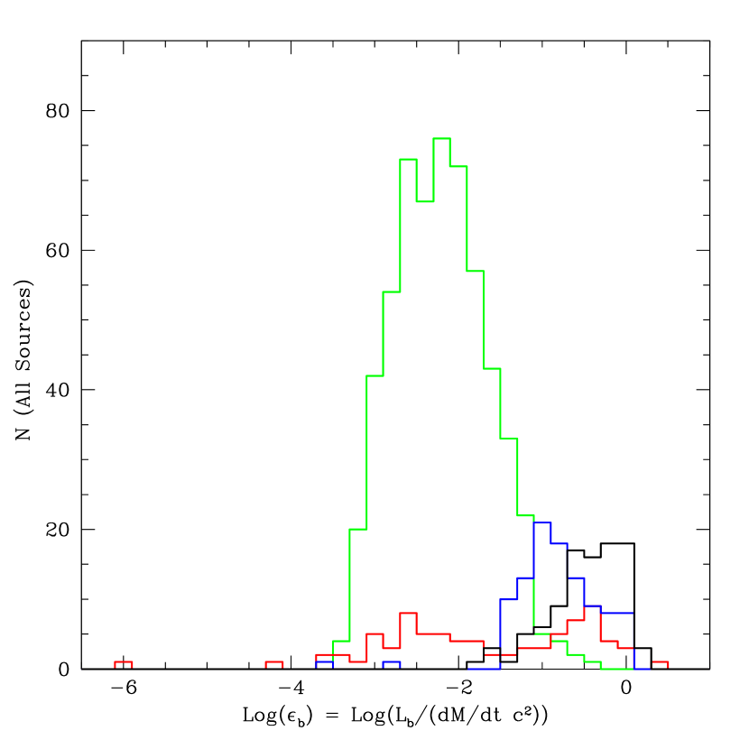
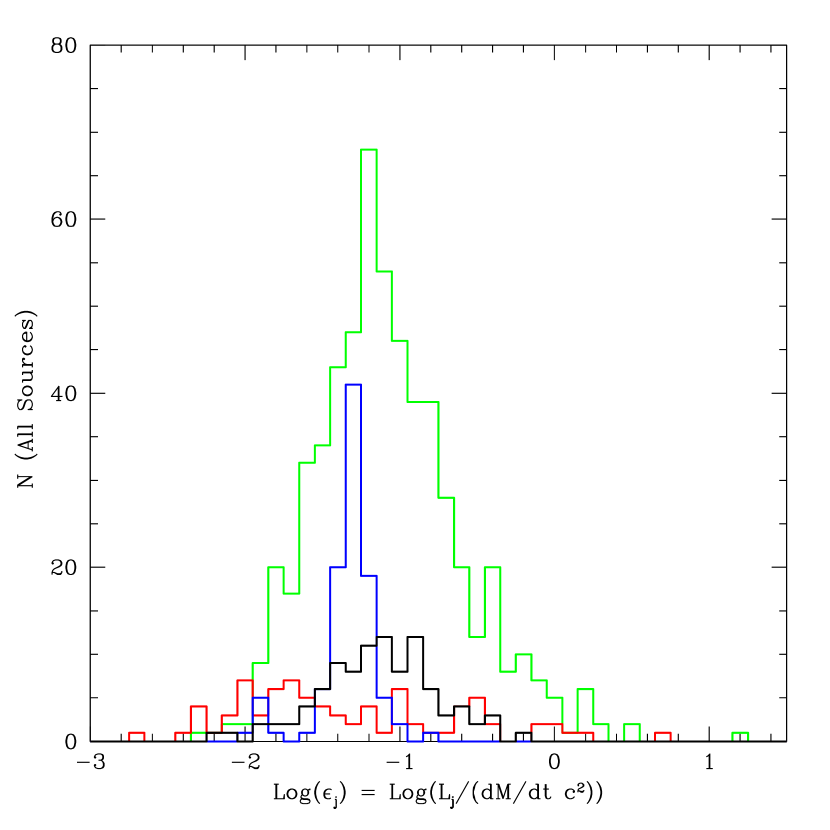
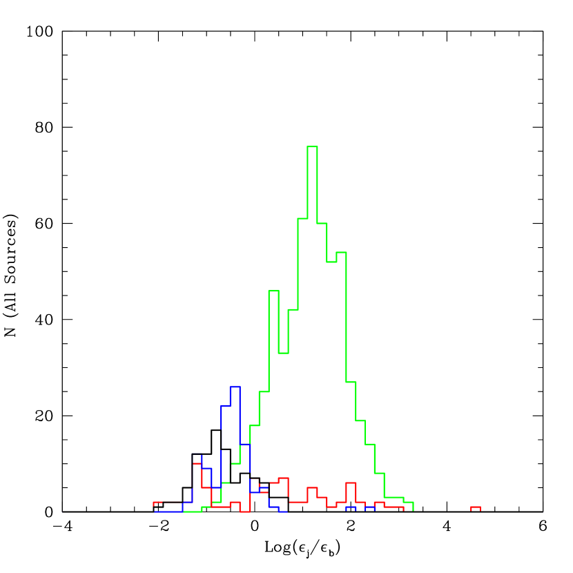
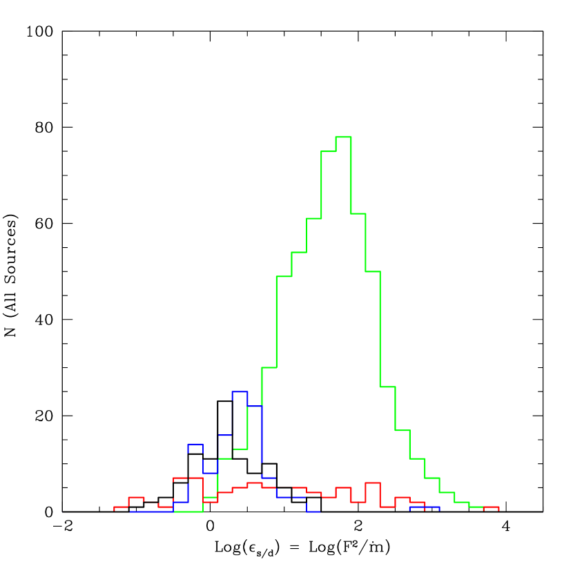
Histograms illustrating the efficiency factors are shown in Figs. 5 - 8. The mean value and dispersion for the efficiency factors , , the ratio , and , defined in section 3.2, are listed in columns (6) - (9) for the samples and sources discussed in section 4.1, as described above.
The efficiency factor for the bolometric luminosity of the accretion disk, shown in Fig. 5 and listed in column (6) of Table 1 indicates a significant overlap of values for the FRII sources and GBH. The M03 local sample of AGN appears to split into two components, with a break at . The higher efficiency factor component is similar to that of the FRII sources, while the lower efficiency factor component is similar to that of the NB16 LINER sample. To study this further, values of for each of the GBH, and different categories of AGN for the FRII and M03 samples are listed in Table 1. The Q, NS1, and S(1-1.9) from the M03 sample overlap with the FRII sources, while the L1.9, L2, and S2 M03 sources overlap with the NB16. A similar trend is seen for the dimensionless mass accretion rates. This is not the case for the mass accretion rates in physical units, where the NB16 LINERs and M03 sample show significant overlap, while the FRII sources and GBH have little overlap with other types of sources. The fact that the mean values of for the samples are quite different, and that the dispersion of each of the samples and subsamples is large, indicates that a constant value of does not provide an accurate description of these sources. Splitting the samples into sub-sets, as shown in Table 1 for the GBH, FRII, and M03 sources may provide a way to estimate for each sub-type. Of course, the entire sample of LINERs is one sub-type of AGN.
The efficiency factor of radiation from the accretion disk, , for some sources studied here were obtained by Raimundo et al. (2012) using methods that are independent of those developed and applied here. Raimundo et al. (2012) used two different methods to obtain bolometric disk luminosities, and the resulting efficiency factors are listed in Tables 2 and 3 of that paper, referred to here as R12(T2) and R12(T3). A comparison of efficiency factors for three sources that are in both R12(T2) and R12(T3) indicate that their efficiency factors internally agree to a factor of about 1.5 - 2. Accretion disk efficiency factors for sources studied here that overlap with those studied by Raimundo et al. (2012) are included in columns (6) - (10) of the second part of Table 2; there (T5) refers to Table 5 (presented here and included below). The ratio of values obtained here to those listed in R12(T2) and R12(T3) are listed in columns (8) and (10) of Table 2, respectively. Most of the sources agree to a factor of a few, which is reasonably good agreement considering that it is similar to the internal consistency of the comparison sample, and considering that the observations used in the different studies were obtained at different times, and the sources may be intrinsically time variable.
The beam power efficiency factors are shown in Fig. 6 and are listed in column (7) of Table 1. These are proportional to (see eq. (10). Remarkably, the mean values of for all of the samples and source types are consistent given the dispersion of each sample. Each AGN sample has a rather broad range of values, which is reflected in the large dispersion of each sample. Thus, though the mean values of are similar for all source samples and types studied, the large dispersion of the AGN samples and sub-types would have to be taken into account before assuming and applying a value for similar sources. The dispersion of the GBH is relatively small, and the values presented here for the GBH could provide a reliable estimate of (i.e. ) for similar sources.
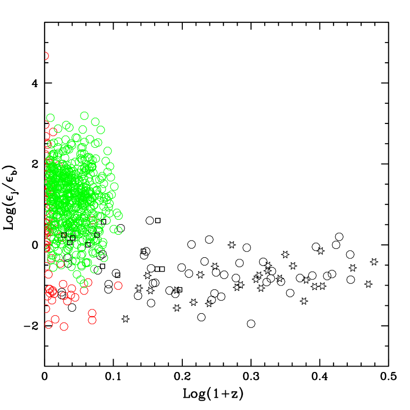
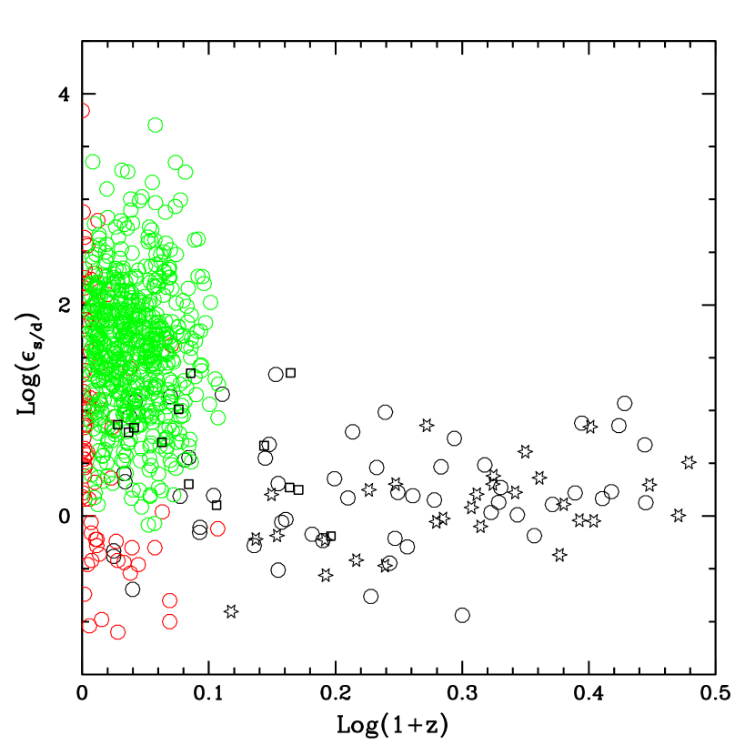
The ratio (i.e. ) is shown in Fig. 7 and values are listed in column (8) of Table 1. The values for the GBH and FRII sources have substantial overlap, and one component of the M03 sources also overlaps with these sources. A long tail of values for the M03 sample overlaps with the NB16 LINERs. This quantity essentially separates sources into disk dominated sources and jet dominated sources. Sources with are jet dominated, and those with are disk dominated (see also D18). Clearly, most of the LINERs and some of the M03 sources are jet dominated, most by a very large factor of 10 to 100. Outflow from these sources are almost certainly powered by black hole spin, as discussed in section 1.1 (see also section 1.1 of D19). Other sources with very large values of this quantity include A0 6200, and the M03 L1.9, L2, and S2 sources. Sources with values less than one include FRII sources of all types, most of the GBH, and the M03 Q, and NS1 sources, while the S(1-1.9) sources have a mean value near 1 and a very large dispersion.
Another measure of interest is the relative input to the Eddington-normalized outflow beam power from black hole spin and from the accretion disk. Eq. (1) may be written as , so one measure of this relative input is given by , defined by eq. (11). Values of this quantity are listed in column (9) of Table 1. Almost all of the sources have values of that are greater than 1. Types that include values less than one include about half of the FRII quasars (Q), the 3 FRII W sources, and some of the M03 Q and NS1 sources. This highlights the role of black hole spin as the source that powers the outflow and that of the accretion disk as the source that maintains the magnetic field that is anchored in the disk and threads the black hole. Note that in the model described by Meier (1999), both a disk wind, as in the model of Blandford & Payne (1982), and spin energy extraction from the black hole, as in the model of Blandford & Znajek 1977, power the outflow, and this model is also described by eq. (1), as discussed in detail by D19 section 4 (see also Meier 1999).
5 Discussion
In addition to considering histograms of quantities, it is helpful view the redshift distributions of the sources to get a sense of contributions to the histograms from sources at different redshift. The GBH are located in the Galaxy, so these are not including in the redshift distributions shown in Figs. 3, 4, and 9-13. The M03 sources are quite local, and include sources with a wide range of intrinsic parameters. The NB16 sources extend to a redshift of about 0.3, with this cutoff imposed by NB16 for this study. The D19 sources extend to a redshift of about 2. For some parameters, it is easy to see the impact of missing lower luminosity sources as redshift increases, while other parameters do not have a strong redshift dependence. For sources that increase with redshift, the upper envelope of the distributions provides a guide as to how parameters that describe the most luminous and radio bright sources evolve with redshift.
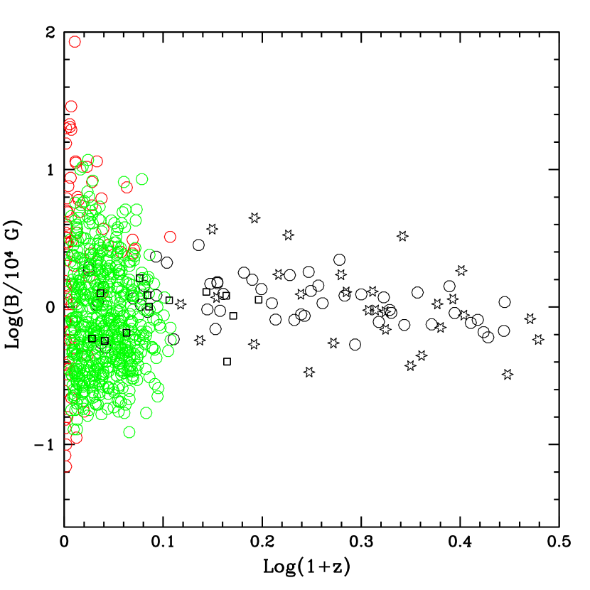
It is clear from Fig. 4 that sources at higher redshift have higher mass accretion rates physical units, so the high mass accretion rates seen in Fig. 2 are due to these sources. The low redshift sample of M03 suggests that there are sources at all accretion rates, and that the lower luminosity sources that are associated with lower mass accretion rates are missing at higher redshift due to the flux limited nature of the samples that include higher redshift sources. Fig. 3 shows the dimensionless mass accretion rate as a function of redshift. Clearly, there is a rather sharp boundary at , and this is not artificially imposed, but is an empirical result and reflects that very sharp boundary found by D16, D18, and D19 when the bolometric disk luminosity approaches the Eddington luminosity. While , the accretion disk magnetic field strength in physical units is obtained from , which accounts for the redshift distribution of FRII sources seen in Fig. 13. This suggests a weak dependence of the disk magnetic field strength, , in physical units on redshift.
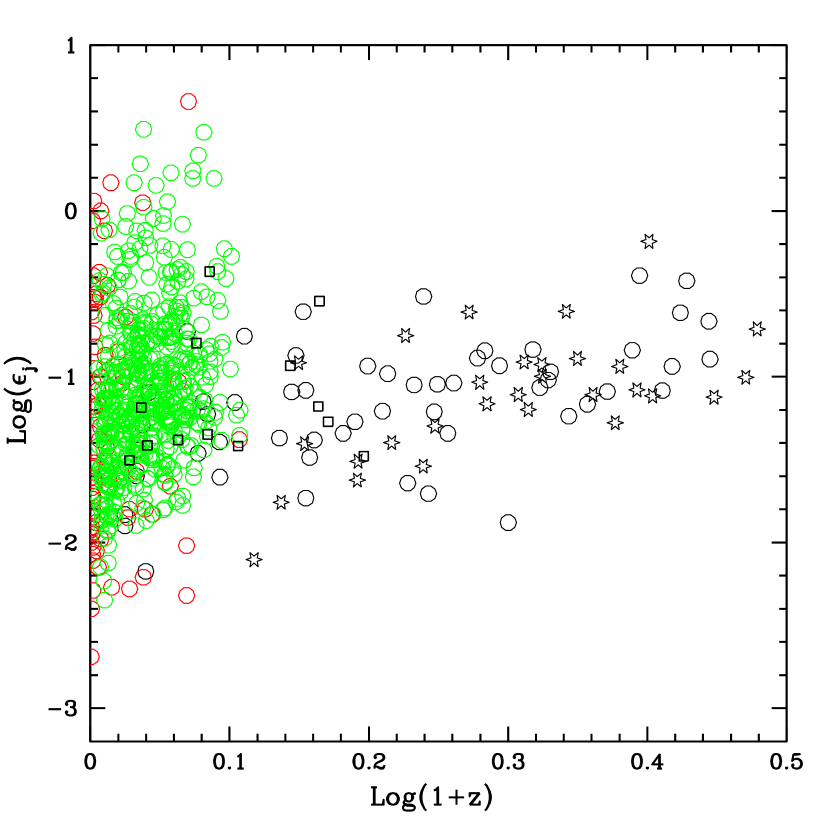
The efficiency factors are shown as a function of redshift in Figs. 9 to 12. Fig. 9 reflects the fact that there are no super-Eddington sources. There is a narrow range of values for the FRII sources with little or no redshift evolution. It is clear that NB16 LINERs with lower values of that are present near zero redshift have dropped out by a redshift of about 0.3, most likely reflecting a selection effect whereby lower luminosity sources are not included in the sample as redshift increases (NB16). Redshift selection effects for and for each sample separately are much less pronounced, especially that for , compared with that for .
6 Summary & Conclusions
The outflow method allows empirical estimates of the accretion disk magnetic field strength in Eddington units, , at the location where the magnetic field that torques the black hole is anchored in the disk (D19). Interestingly, two key physical parameters describing the accretion disk can be obtained from this ratio: the magnetic field strength in physical units, and the mass accretion rate in physical units. As shown in sections 1.1 and 3.1, the mass accretion rate in physical units is , whereas the accretion disk magnetic field strength in physical units is (D19). So, three important physical quantities that describe the accretion disk follow from empirical estimates of : the dimensionless mass accretion rate; the mass accretion rate in physical units; and the disk magnetic field strength in physical units (disk magnetic pressure in physical units). Here, data for three samples of AGN, including 756 supermassive black hole systems, and 103 measurements of 4 stellar mass black holes, referred to as GBH, are used to obtain and study mass accretion rates and efficiency factors, while the magnetic field strength in physical and dimensionless units are discussed by D19.
Mass accretion rates in dimensionless units can be divided into five categories, defined here as high (, medium-high (, medium (, medium-low (, and low . Broadly, sources fall into the following categories: all FRII sources (except LEG), and M03 NS1 and Q sources have high ; three GBH (all except A06200), the D16/19 FRII LEG, and the M03 S(1-1.9) sources have medium-high ; the M03 S2 sources have medium ; GBH A0 6200, the NB16 LINERs, and M03 L1.9 and L2 sources have medium-low ; a few individual sources have low (see Tables 3-6).
Mass accretion rates in physical units for the AGN studied here seem to have distinct mean values, but with a broad dispersion, as is evident in Fig. 2, and appear to fall into four broad categories: high, medium, low, and very low. Sources with high mass accretion rates, where is in units of , have () and include FRII Q and some HEG; sources with medium rates of about include FRII LEG, W, and some HEG types and M03 Q types; sources with mean values in the low range from are practically absent; and sources with very low rates of about () include the NB16 LINERs and all of the M03 sources except Q type. Though sources with mean values in the low range are practically absent, many individual sources fall into this range and are evident in the dispersion of the mean values of . The GBH all have very similar mass accretion rates of about , with a few individual observations stretching to very low values of about , for example one observation of A0 6200 and one of V404 Cyg (see Table 3).
Efficiency factors associated with the bolometric luminosity of the accretion disk have a broad range, and may be categorized as high , medium , and low . Sources with high values include most or all of the FRII sources (except about half of the FRII LEG, which fall into the medium category), GX 339-4, about half of the observations of V404 Cyg, and the M03 NS1 and Q sources. Sources in the medium category include about half of the FRII LEG sources and about half of the V404 Cyg observations, J1118+480, and the M03 S(1-1.9) and S2 types. Sources in the low category include the NB16 LINERs, A0 6200, and the M03 L1.9 and L2 types.
The mean values of efficiency factors associated with collimated outflows, , defined in the traditional manner in terms of mass accretion rate, have a small range of mean values and a large dispersion per sample (see the first four lines of Table 1 and Fig. 6). This efficiency factor measures the beam power relative to the mass accretion rate in physical units. In the spin powered outflow model described in section 1.1, the accretion disk plays the role of maintaining the magnetic field; the field is anchored in the disk and threads the black hole, exerting a torque and producing the outflow (Blandford & Znajek 1977), while it is the spin energy of the hole that powers the outflow. In the Meier model (1999), the outflow is powered by both the spin of the black hole and a disk wind, with the disk wind component similar to that of Blandford & Payne model (1982). The Meier model has the same functional form as the Blandford & Znajek model, but has a different constant of proportionality, and thus is described by eq. (1), as discussed in detail by D19.
A measure of the outflow power sourced to the black hole spin relative to that contributed by the disk is the efficiency factor , listed in column (9) of Table 1. All of the samples, and most of the sub-samples, have mean values of , indicating that most of the outflow beam power originates from the black hole spin. The exceptions are the 3 FRII W sources, and a subset of the 20 M03 NS1 and Q sources.
The ratio was studied in detail by D18. As discussed in that work, sources with are jet dominated sources, while those with are disk dominated sources. The results obtained by D18 align quite well with previously published results, such as those discussed by Heckman & Best (2014) and NB16. The results obtained here indicate that both disk-dominated and jet-dominated sources have outflow beam powers with a spin term that exceeds the disk term, indicated by a value of . That is, almost all of the sources with have , and many sources with have including three of the GBH, all of the FRII sources except the W types, and almost all of the M03 types except NS1 and Q.
Parameters with a dispersion that is not too large could provide estimates of this parameter for additional sources of the same type. If the parameter evolves with redshift, then this should only be applied to sources of the same type within a similar redshift range. To identify such source types, consider quantities with a dispersion less than about 0.5 dex to one significant figure. This suggests that the quantities that could be applied to other sources of the same type are: for NB16 LINERs, , , and ; for FRII sources, , , , and ; for M03 sources, none for the full sample but may be applied to sub-samples; for the GBH, , , , , and . The results obtained here suggest that black hole systems with powerful outflows provide an interesting and important guide for mass accretion rates and efficiency factors that may be applied to additional sources for some source types.
Data Availability Statement
The data underlying this article are available in the article or are listed in D19.
Acknowledgments
Thanks are extended to the referee for very helpful comments and suggestions. It is a pleasure to thank the many colleagues with whom this work was discussed, especially Jean Brodie, George Djorgovski, Megan Donahue, Yan-Fei Jiang, Syd Meshkov, Chiara Mingarelli, Chris O’Dea, Masha Okounkova, David Spergel, Alan Weinstein, and Rosie Wyse. I would especially like to thank Jerry Ostriker for helpful discussions related to the topics discussed in this paper. The Flatiron Institute is supported by the Simons Foundation. This work was also supported in part by the Losoncy Fund and the PSU Berks Advisory Board, and was performed in part at the Aspen Center for Physics, which is supported by National Science Foundation grant PHY-1607611.
| (1) | (2) | (3) | (4) | (5) | (6) | (7) | (8) | (9) | (10) |
|---|---|---|---|---|---|---|---|---|---|
| Sample | type | N | () | () | () | ( | () | ||
| or Source | |||||||||
| NB16 | AGN | ||||||||
| D16/D19 | AGN | ||||||||
| M03 | AGN | ||||||||
| S15 | GBH | ||||||||
| GX 339-4 | GBH | ||||||||
| V404 Cyg | GBH | ||||||||
| J1118+480 | GBH | ||||||||
| A0 6200 | GBH | ||||||||
| FRII | W | ||||||||
| FRII | Q | ||||||||
| FRII | HEG | ||||||||
| FRII | LEG | ||||||||
| M03 | NS1 | ||||||||
| M03 | Q | ||||||||
| M03 | S(1-1.9) | ||||||||
| M03 | S2 | ||||||||
| M03 | L1.9 | ||||||||
| M03 | L2 |
| (1) | (2) | (3) | (4) | (5) | |||||
|---|---|---|---|---|---|---|---|---|---|
| Source | Type | J19 | This Work (T5) | Ratio | |||||
| (T5)/J19 | |||||||||
| Ark | NS1 | ||||||||
| Mrk | S1.5 | ||||||||
| Mrk | NS1 | ||||||||
| Mrk | S1.2 | ||||||||
| PG | Q | ||||||||
| PG | Q | ||||||||
| PG | Q | ||||||||
| PG | Q | ||||||||
| (1) | (2) | (3) | (4) | (5) | (6) | (7) | (8) | (9) | (10) |
| Source | Type | R12 (T1) | This Work (T5) | Ratio | R12 (T3) | This Work (T5) | Ratio | R12 (T2) | Ratio |
| (T5)/R12(T1) | (T5)/R12(T3) | (T5)/R12(T2) | |||||||
| Mrk | S1.5 | ||||||||
| Mrk | NS1 | ||||||||
| NGC | S1.5 | ||||||||
| NGC | S1 | ||||||||
| 3C | S1 | ||||||||
| 3C | S1 |
| (1) | (2) | (3) | (4) | (5) | (6) | (7) | (8) |
|---|---|---|---|---|---|---|---|
| Source | () | () | () | () | () | ||
| GX | |||||||
| GX | |||||||
| GX | |||||||
| GX | |||||||
| GX | |||||||
| GX | |||||||
| GX | |||||||
| GX | |||||||
| GX | |||||||
| GX | |||||||
| GX | |||||||
| GX | |||||||
| GX | |||||||
| GX | |||||||
| GX | |||||||
| GX | |||||||
| GX | |||||||
| GX | |||||||
| GX | |||||||
| GX | |||||||
| GX | |||||||
| GX | |||||||
| GX | |||||||
| GX | |||||||
| GX | |||||||
| GX | |||||||
| GX | |||||||
| GX | |||||||
| GX | |||||||
| GX | |||||||
| GX | |||||||
| GX | |||||||
| GX | |||||||
| GX | |||||||
| GX | |||||||
| GX | |||||||
| GX | |||||||
| GX | |||||||
| GX | |||||||
| GX | |||||||
| GX | |||||||
| GX | |||||||
| GX | |||||||
| GX | |||||||
| GX | |||||||
| GX | |||||||
| GX | |||||||
| GX | |||||||
| GX | |||||||
| GX | |||||||
| GX | |||||||
| GX | |||||||
| GX | |||||||
| GX | |||||||
| GX | |||||||
| GX | |||||||
| GX | |||||||
| GX | |||||||
| GX | |||||||
| GX | |||||||
| GX | |||||||
| GX | |||||||
| GX | |||||||
| GX | |||||||
| GX | |||||||
| GX | |||||||
| GX | |||||||
| GX | |||||||
| GX | |||||||
| GX | |||||||
| GX | |||||||
| GX | |||||||
| GX | |||||||
| GX | |||||||
| GX | |||||||
| GX |
Mass Accretion Rates and Efficiency Factors for Stellar-Mass Galactic Black Holes in X-ray Binary Systems. (1) (2) (3) (4) (5) (6) (7) (8) Source () () () () () XTE XTE XTE XTE XTE V404 Cyg V404 Cyg V404 Cyg V404 Cyg V404 Cyg V404 Cyg V404 Cyg V404 Cyg V404 Cyg V404 Cyg V404 Cyg V404 Cyg V404 Cyg V404 Cyg V404 Cyg V404 Cyg V404 Cyg V404 Cyg V404 Cyg V404 Cyg A0 6200 A0 6200
| (1) | (2) | (3) | (4) | (5) | (6) | (7) | (8) | (9) | (10) |
|---|---|---|---|---|---|---|---|---|---|
| Source | type | z | () | () | () | () | () | ||
| 3C 33 | HEG | ||||||||
| 3C 192 | HEG | ||||||||
| 3C 285 | HEG | ||||||||
| 3C 452 | HEG | ||||||||
| 3C 388 | HEG | ||||||||
| 3C 321 | HEG | ||||||||
| 3C 433 | HEG | ||||||||
| 3C 20 | HEG | ||||||||
| 3C 28 | HEG | ||||||||
| 3C 349 | HEG | ||||||||
| 3C 436 | HEG | ||||||||
| 3C 171 | HEG | ||||||||
| 3C 284 | HEG | ||||||||
| 3C 300 | HEG | ||||||||
| 3C 438 | HEG | ||||||||
| 3C 299 | HEG | ||||||||
| 3C 42 | HEG | ||||||||
| 3C 16 | HEG | ||||||||
| 3C 274.1 | HEG | ||||||||
| 3C 457 | HEG | ||||||||
| 3C 244.1 | HEG | ||||||||
| 3C 46 | HEG | ||||||||
| 3C 341 | HEG | ||||||||
| 3C 172 | HEG | ||||||||
| 3C 330 | HEG | ||||||||
| 3C 49 | HEG | ||||||||
| 3C 337 | HEG | ||||||||
| 3C 34 | HEG | ||||||||
| 3C 441 | HEG | ||||||||
| 3C 247 | HEG | ||||||||
| 3C 277.2 | HEG | ||||||||
| 3C 340 | HEG | ||||||||
| 3C 352 | HEG | ||||||||
| 3C 263.1 | HEG | ||||||||
| 3C 217 | HEG | ||||||||
| 3C 175.1 | HEG | ||||||||
| 3C 289 | HEG | ||||||||
| 3C 280 | HEG | ||||||||
| 3C 356 | HEG | ||||||||
| 3C 252 | HEG | ||||||||
| 3C 368 | HEG | ||||||||
| 3C 267 | HEG | ||||||||
| 3C 324 | HEG | ||||||||
| 3C 266 | HEG | ||||||||
| 3C 13 | HEG | ||||||||
| 4C 13.66 | HEG | ||||||||
| 3C 437 | HEG | ||||||||
| 3C 241 | HEG | ||||||||
| 3C 470 | HEG | ||||||||
| 3C 322 | HEG | ||||||||
| 3C 239 | HEG | ||||||||
| 3C 294 | HEG | ||||||||
| 3C 225B | HEG | ||||||||
| 3C 55 | HEG | ||||||||
| 3C 68.2 | HEG |
Mass Accretion Rates and Efficiency Factors for the Classical Double (FRII) Sources. (1) (2) (3) (4) (5) (6) (7) (8) (9) (10) Source type z () () () () () 3C 35 LEG 3C 326 LEG 3C 236 LEG 4C 12.03 LEG 3C 319 LEG 3C 132 LEG 3C 123 LEG 3C 153 LEG 4C 14.27 LEG 3C 200 LEG 3C 295 LEG 3C 19 LEG 3C 427.1 LEG 3C 249.1 Q 3C 351 Q 3C 215 Q 3C 47 Q 3C 334 Q 3C 275.1 Q 3C 263 Q 3C 207 Q 3C 254 Q 3C 175 Q 3C 196 Q 3C 309.1 Q 3C 336 Q 3C 245 Q 3C 212 Q 3C 186 Q 3C 208 Q 3C 204 Q 3C 190 Q 3C 68.1 Q 4C 16.49 Q 3C 181 Q 3C 268.4 Q 3C 14 Q 3C 270.1 Q 3C 205 Q 3C 432 Q 3C 191 Q 3C 9 Q 3C 223 W 3C 79 W 3C 109 W
| (1) | (2) | (3) | (4) | (5) | (6) | (7) | (8) | (9) | (10) |
|---|---|---|---|---|---|---|---|---|---|
| Source | type | D(Mpc) | () | () | () | () | () | ||
| Ark | NS1 | ||||||||
| Cyg | S2/L2 | ||||||||
| IC | L2 | ||||||||
| IC | L1.9 | ||||||||
| IC | S1 | ||||||||
| Mrk | S2 | ||||||||
| Mrk | S1.5 | ||||||||
| Mrk | NS1 | ||||||||
| Mrk | S2 | ||||||||
| Mrk | NS1 | ||||||||
| Mrk | NS1 | ||||||||
| Mrk | NS1 | ||||||||
| Mrk | S1.2 | ||||||||
| Mrk | NS1 | ||||||||
| NGC | L1.9 | ||||||||
| NGC | L1.9 | ||||||||
| NGC | S1.9 | ||||||||
| NGC | S2 | ||||||||
| NGC | S1.8 | ||||||||
| NGC | S2 | ||||||||
| NGC | S2 | ||||||||
| NGC | S2 | ||||||||
| NGC | S2 | ||||||||
| NGC | L1.9 | ||||||||
| NGC | L2 | ||||||||
| NGC | S2 | ||||||||
| NGC | S1.5 | ||||||||
| NGC | S2 | ||||||||
| NGC | S2 | ||||||||
| NGC | L2 | ||||||||
| NGC | L1.9 | ||||||||
| NGC | S1.5 | ||||||||
| NGC | S1 | ||||||||
| NGC | L1.9 | ||||||||
| NGC | NS1 | ||||||||
| NGC | S2 | ||||||||
| NGC | L1.9 | ||||||||
| NGC | S1.5 | ||||||||
| NGC | L1.9 | ||||||||
| NGC | S1.9 | ||||||||
| NGC | L2 | ||||||||
| NGC | L1.9 | ||||||||
| NGC | L2 | ||||||||
| NGC | S2 | ||||||||
| NGC | L1.9 | ||||||||
| NGC | L2 | ||||||||
| NGC | S2 | ||||||||
| NGC | L2 | ||||||||
| NGC | S1.9 | ||||||||
| NGC | S1.9 | ||||||||
| NGC | L2 | ||||||||
| NGC | L2 | ||||||||
| NGC | S1.5 | ||||||||
| NGC | S2 | ||||||||
| NGC | S2 | ||||||||
| NGC | S2 | ||||||||
| NGC | S1.5 | ||||||||
| NGC | S2 | ||||||||
| NGC | S2 | ||||||||
| NGC | S2 | ||||||||
| NGC | L2 | ||||||||
| NGC | S1 | ||||||||
| NGC | S2 | ||||||||
| NGC | S2 | ||||||||
| PG | Q | ||||||||
| PG | Q | ||||||||
| PG | Q | ||||||||
| PG | Q | ||||||||
| PG | Q | ||||||||
| PG | Q | ||||||||
| PG | Q | ||||||||
| PG | Q | ||||||||
| PG | Q | ||||||||
| PG | Q | ||||||||
| PG | Q |
Mass Accretion Rates and Efficiency Factors for the M03 Local Sample of AGN. (1) (2) (3) (4) (5) (6) (7) (8) (9) (10) Source type D(Mpc) () () () () () PG Q PG Q 3C S1 3C S1 Sgr
| (1) | (2) | (3) | (4) | (5) | (6) | (7) | (8) | (9) |
|---|---|---|---|---|---|---|---|---|
| NB16 | ||||||||
| Id | z | |||||||
| 1 | ||||||||
| 2 | ||||||||
| 3 | ||||||||
| 4 | ||||||||
| 5 | ||||||||
| 6 | ||||||||
| 7 | ||||||||
| 8 | ||||||||
| 9 | ||||||||
| 10 | ||||||||
| 11 | ||||||||
| 12 | ||||||||
| 13 | ||||||||
| 14 | ||||||||
| 15 | ||||||||
| 16 | ||||||||
| 17 | ||||||||
| 18 | ||||||||
| 19 | ||||||||
| 20 | ||||||||
| 21 | ||||||||
| 22 | ||||||||
| 23 | ||||||||
| 24 | ||||||||
| 25 | ||||||||
| 26 | ||||||||
| 27 | ||||||||
| 28 | ||||||||
| 29 | ||||||||
| 30 | ||||||||
| 31 | ||||||||
| 32 | ||||||||
| 33 | ||||||||
| 34 | ||||||||
| 35 | ||||||||
| 36 | ||||||||
| 37 | ||||||||
| 38 | ||||||||
| 39 | ||||||||
| 40 | ||||||||
| 41 | ||||||||
| 42 | ||||||||
| 43 | ||||||||
| 44 | ||||||||
| 45 | ||||||||
| 46 | ||||||||
| 47 | ||||||||
| 48 | ||||||||
| 49 | ||||||||
| 50 | ||||||||
| 51 | ||||||||
| 52 | ||||||||
| 53 | ||||||||
| 54 | ||||||||
| 55 | ||||||||
| 56 | ||||||||
| 57 | ||||||||
| 58 | ||||||||
| 59 |
Mass Accretion Rates and Efficiency Factors for the NB16 LINERs. (1) (2) (3) (4) (5) (6) (7) (8) (9) NB16 Id z 60 61 62 63 64 65 66 67 68 69 70 71 72 73 74 75 76 77 78 79 80 81 82 83 84 85 86 87 88 89 90 91 92 93 94 95 96 97 98 99 100 101 102 103 104 105 106 107 108 109 110 111 112 113 114 115 116 117 118 119 120
Mass Accretion Rates and Efficiency Factors for the NB16 LINERs. (1) (2) (3) (4) (5) (6) (7) (8) (9) NB16 Id z 121 122 123 124 125 126 127 128 129 130 131 132 133 134 135 136 137 138 139 140 141 142 143 144 145 146 147 148 149 150 151 152 153 154 155 156 157 158 159 160 161 162 163 164 165 166 167 168 169 170 171 172 173 174 175 176 177 178 179 180
Mass Accretion Rates and Efficiency Factors for the NB16 LINERs. (1) (2) (3) (4) (5) (6) (7) (8) (9) NB16 Id z 181 182 183 184 185 186 187 188 189 190 191 192 193 194 195 196 197 198 199 200 201 202 203 204 205 206 207 208 209 210 211 212 213 214 215 216 217 218 219 220 221 222 223 224 225 226 227 228 229 230 231 232 233 234 235 236 237 238 239 240
Mass Accretion Rates and Efficiency Factors for the NB16 LINERs. (1) (2) (3) (4) (5) (6) (7) (8) (9) NB16 Id z 241 242 243 244 245 246 247 248 249 250 251 252 253 254 255 256 257 258 259 260 261 262 263 264 265 266 267 268 269 270 271 272 273 274 275 276 277 278 279 280 281 282 283 284 285 286 287 288 289 290 291 292 293 294 295 296 297 298 299 300 301
Mass Accretion Rates and Efficiency Factors for the NB16 LINERs. (1) (2) (3) (4) (5) (6) (7) (8) (9) NB16 Id z 302 303 304 305 306 307 308 309 310 311 312 313 314 315 316 317 318 319 320 321 322 323 324 325 326 327 328 329 330 331 332 333 334 335 336 337 338 339 340 341 342 343 344 345 346 347 348 349 350 351 352 353 354 355 356 357 358 359 360 361
Mass Accretion Rates and Efficiency Factors for the NB16 LINERs. (1) (2) (3) (4) (5) (6) (7) (8) (9) NB16 Id z 362 363 364 365 366 367 368 369 370 371 372 373 374 375 376 377 378 379 380 381 382 383 384 385 386 387 388 389 390 391 392 393 394 395 396 397 398 399 400 401 402 403 404 405 406 407 408 409 410 411 412 413 414 415 416 417 418 419 420 421 422
Mass Accretion Rates and Efficiency Factors for the NB16 LINERs. (1) (2) (3) (4) (5) (6) (7) (8) (9) NB16 Id z 423 424 425 426 427 428 429 430 431 432 433 434 435 436 437 438 439 440 441 442 443 444 445 446 447 448 449 450 451 452 453 454 455 456 457 458 459 460 461 462 463 464 465 466 467 468 469 470 471 472 473 474 475 476 477 478 479 480 481 482
Mass Accretion Rates and Efficiency Factors for the NB16 LINERs. (1) (2) (3) (4) (5) (6) (7) (8) (9) NB16 Id z 483 484 485 486 487 488 489 490 491 492 493 494 495 496 497 498 499 500 501 502 503 504 505 506 507 508 509 510 511 512 513 514 515 516 517 518 519 520 521 522 523 524 525 526 527 528 529 530 531 532 533 534 535 536 537 538 539 540 541 542 543 544
Mass Accretion Rates and Efficiency Factors for the NB16 LINERs. (1) (2) (3) (4) (5) (6) (7) (8) (9) NB16 Id z 545 546 547 548 549 550 551 552 553 554 555 556 557 558 559 560 561 562 563 564 565 566 567 568 569 570 571 572 573 574 575 576
References
- Bian & Zhao (2003) Bian, W-H., & Zhao, Y-H. 2003, PASJ, 55, 599
- Begelman et al. (1984) Begelman, M. C., Blandford, R. D., & Rees, M. J. 1984, RvMp, 56, 255
- Blandford (1990) Blandford, R. D. 1990, in Active Galactic Nuclei, ed. T. J. L. Courvoisier & M. Mayor (Berlin: Springer), 161
- Blandford & Payne (1982) Blandford, R. D., & Payne, D. G. 1982, MNRAS, 199, 883
- Blandford & Znajek (1977) Blandford, R. D., & Znajek, R. L. 1977, MNRAS, 179, 433
- Corbel et al. (2013) Corbel S., Coriat M., Brocksopp C., Tzioumis A. K., Fender R. P., Tomsick J. A., Buxton M. M., & Bailyn C. D., 2013, MNRAS, 428, 2500
- Corbel et al. (2008) Corbel S., Körding E., Kaaret P., 2008, MNRAS, 389, 1697
- Daly (2009) Daly, R. A. 2009, ApJL, 696, L32
- Daly (2011) Daly, R. A. 2011, MNRAS, 414, 1253
- Daly (2016) Daly, R. A. 2016, MNRAS 458, L24
- Daly (2019) Daly, R. A. 2019, ApJ, 886, 37
- Daly & Sprinkle (2014) Daly, R. A., & Sprinkle, T. B. 2014, MNRAS, 438, 3233
- Daly et al. (2012) Daly, R. A., Sprinkle, T. B., O’Dea, C. P., Kharb, P., & Baum, S. A. 2012, MNRAS, 423, 2498
- Daly et al. (2018) Daly, R. A., Stout, D. A., Mysliwiec, J. N. 2018, ApJ, 863, 117
- Davis & Laor (2011) Davis, S. W., Laor, A., 2011, ApJ, 728, 98
- Dermer et al. (2008) Dermer, C., Finke, J., & Menon, G. 2008, Black-Hole Engine Kinematics, Flares from PKS2155-304, and Multiwavelength Blazar Analysis (Trieste: SISSA)
- Dicken et al. (2014) Dicken, D., Tadhunter, C., Morganti, R., Axon, D., Robinson, A., Magagnoli, M., Kharb, P., Ramos Almeida C., Mingo, B., Hardcastle, M., Nesvadba, N. P. H., Singh, V., Kouwenhoven, M. B. N., Rose, M., Spoon, H., Inskip, K. J., & Holt, J. 2014, ApJ, 788, 98
- Fernandes et al. (2015) Fernandes, C. A. C., Jarvis, M. J., Martínez-Sansigre, A., Rawlings, S., Afonso, J., Hardcastle, M. J., Lacy, M., Stevens, J. A., Vardoulaki, E. 2015, MNRAS, 447, 1184
- Gallo et al. (2006) Gallo E., Fender R. P., Miller-Jones J. C. A., Merloni A., Jonker P. G., Heinz S., Maccarone T. J., & van der Klis M., 2006, MNRAS, 370, 13511360
- Gelino et al. (2001) Gelino D. M., Harrison T. E., & Orosz J. E., 2001, AJ, 122, 2668
- Gou et al. (2010) Gou, L., McClintock, J. E., Steiner, J. F., Narayan, R., Cantrell, A. G., & Bailyn, C. D. 2010, ApJL, 718, L122
- Grimes, Rawlings, & Willott (2004) Grimes, J. A., Rawlings, S., & Willott, C. J. 2004, MNRAS, 349, 503
- Heckman & Best (2014) Heckman, T. M., & Best, P. N. 2014, ARA&A, 52, 589
- Heckman et al. (2004) Heckman, T. M., Kauffmann, G., Brinchmann, J., Charlot, S., Tremonti, C., & White, S. D. M. 2004, ApJ, 613, 109
- Ho (2009) Ho, L. C. 2009, ApJ, 699, 626
- Jiang et al. (2019) Jiang, J., Fabian, A. C., Dauser, T., Gallo, L., García, J. A., Kara, E., Parker, M. L., Tomsick, J. A., Walton, D. J., & Reynolds, C. S. 2019, MNRAS, 489, 3436
- Jonker et al. (2004) Jonker P., & Nelemans G., 2004, MNRAS, 354, 355
- Kuulkers et al. (1999) Kuulkers, E., Fender, R. P., Spencer, R. E., Davis, R. J., & Morison, I. 1999, MNRAS, 306, 919
- Lasota (2000) Lasota, J. -P. 2000, A&A, 360, 575
- McClintoch et al. (2003) McClintock, J. E., Narayan, R., Garcia, M. R., Orosz, J. A., Remillard, R. A., & Murray, S. S. 2003, ApJ, 593, 435
- McLure et al. (2006) McLure, R. J., Jarvis, M. J., Targett, T. A., Dunlop, J. S., & Best, P. N. 2006, MNRAS, 368, 1395
- McLure et al. (2004) McLure, R. J., Willott, C. J., Jarvis, M. J., Rawlings, S., Hill, G. J., Mitchell, E., Dunlop, J. S., & Wold, M. 2004, MNRAS, 351, 347
- Meier (1999) Meier, D. L. 1999, ApJ, 522, 753
- Merloni et al. (2003) Merloni A., Heinz S., & di Matteo T., 2003, MNRAS, 345, 1057
- Mingo et al. (2014) Mingo, B., Hardcastle, M. J., Croston, J. H., Dicken, D., Evans, D. A., Morganti, R., & Tadhunter, C. 2014, MNRAS, 440, 269
- Narayan & McClintock (2012) Narayan, R., & McClintock, J. E. 2012, MNRAS, 419, L69
- Netzer & Trakhtenbrot (2014) Netzer, H., & Trakhtenbrot, B. 2014, MNRAS, 438, 672
- Nisbet & Best (2016) Nisbet, D. M., & Best, P. N. 2016, MNRAS, 455, 2551
- O’Dea et al. (2009) O’Dea, C. P., Daly, R. A., Freeman, K. A., Kharb, P., & Baum, S. 2009, A&A, 494, 471
- O’Dea & Saikia (2020) O’Dea, C. P., Saikia, D. J. 2020, arXiv:2009.02750
- Owen et al. (1976) Owen, F. N., Balonek, T. J., Dickey, J., Terzian, Y., & Gottesman, S. T. 1976, ApJ, 203, L15
- Raimundo et al. (2012) Raimundo, S. I., Fabian, A. C., Vasudevan, R. V., Gandhi, P., & Wu, J. 2012, MNRAS, 419, 2529
- Rees (1984) Rees, M. J. 1984, ARA&A, 22, 471
- Saikia et al. (2015) Saikia P., Körding E., & Falcke H., 2015, MNRAS, 450, 2317
- Sesana et al. (2014) Sesana, A., Barausse, E., Dotti, M., & Rossi, E. M. 2014, ApJ, 794, 104
- Shahbaz et al. (1996) Shahbaz T., Bandyopadhyay R., Charles P. A., & Naylor T., 1996, MNRAS, 282, 977
- Shahbaz et al. (1994) Shahbaz T., Naylor T., & Charles P. A., 1994, MNRAS, 268, 756
- Shakura & Sunyaev (1973) Shakura, N. I., & Sunyaev, R. A. 1973, A&A, 24, 337
- Shao & Li (2020) Shao, Y., & Li, X-D., 2020, arXiv:2006.15961
- Skipper & McHardy (2016) Skipper, C. J., & McHardy, I. M. 2016, MNRAS, 458, 1696
- Trakhtenbrot (2014) Trakhtenbrot, B. 2014, ApJ, 789, L9
- Trakhtenbrot et al. (2017) Trakhtenbrot, B., Volonteri, M., Natarajan, P. 2014, ApJ, 836, L1
- Wu, Lu, & Zhang (2013) Wu, S., Lu, Y., & Zhang, F. 2013, MNRAS, 436, 4271
- Yuan & Narayan (2014) Yuan, F., & Narayan, R. 2014, ARA&A, 52, 529
- Zdziarski et al. (2019) Zdziarski, A. A., Ziolkowski, J., & Mikolajewska, J. 2019, MNRAS, 488, 1026
- Ziolkowski & Zdziarski (2018) Ziolkowski, J., & Zdziarski, A. A. 2018, MNRAS, 480, 1580
- Zycki et al. (1999) Zycki P. T., Done C., & Smith D. A., 1999, MNRAS, 305, 231