Bending of pinned dust ion acoustic solitary waves in presence of charged space debris

Abstract

We consider a low temperature plasma environment in the Low Earth Orbital (LEO) region in presence of charged space debris particles. The dynamics of (2+1) dimensional nonlinear dust ion acoustic waves with weak transverse perturbation, generated in the system is found to be governed by a forced Kadomtsev-Petviashvili (KP) equation, where the forcing term depends on charged space debris function. The bending phenomena of some exact dust ion acoustic solitary wave solutions in $x-t$ and $x-y$ plane are shown; that are resulted from consideration of different types of possible localized debris functions. A family of exact pinned accelerated solitary wave solutions has been obtained where the velocity changes over time but the amplitude remains constant. The shape of debris function also changes during its propagation. Also, a special exact solitary wave solution has been derived for the dust ion acoustic wave; that gets curved in spatial dimensions with the curvature depending upon nature of forcing debris function. Such intricate solitary wave solutions may be useful in modelling real experimental data.

I Introduction

Upsurge in the research on space plasma physics has began and achieved importance from middle of last century Spaceplasma . As a result, near-Earth space has become a virtual laboratory to study different physical properties of astronomical plasma system. In this context, the research on dynamics of space debris objects has also increased drastically Klinkrad ; Sampaio ; Kulikov .

Space debris objects Klinkrad include dead satellites, meteoroids, destroyed spacecrafts and other inactive materials resulting from many natural phenomena etc.; which are being levitated in extraterrestrial regions especially in near-Earth space. The space debris objects are substantially found in the Low Earth Orbital (LEO) and Geosynchronous Earth Orbital (GEO) regions Sampaio . Also, their number is continuously increasing nowadays due to various artificial space missions which result in dead satellites, destroyed spacecrafts etc. The debris particles become charged in a plasma medium because of different mechanisms such as photo-emission, electron and ion collection, secondary electron emission Horanyi etc. These charged debris particles of varying sizes ( as small as microns to as big as centimeters) Sen ; NASA move with different velocities causing significant harm to running spacecrafts. Therefore, to avoid these deteriorating effects, active debris removal (ADR) has become a challenging problem in twenty-first century. Some indirect detection techniques for space debris objects have also been developed by different authors Kulikov ; Sen ; AcharyaHall . A new detection technique for charged debris objects in the LEO region was proposed by Sen et al Sen making use of the interaction of nonlinear plasma waves with charged space debris. They considered the dynamics of nonlinear ion acoustic waves in (1+1) dimensions and derived a forced KdV equation where the forcing term depends on the debris function. Considering a Gaussian debris function, they have predicted “precursor solitons”, that are emitted periodically, through numerical computation. Such precursors can be detected by appropriate sensors to give an indirect evidence of the existence of charged space debris objects. Numerical techniques Sen1 have confirmed the existence of the pinned and precursor solitons even in the large amplitude generalization of the problem. Molecular dynamic simulations for a charged object moving at a supersonic speed in a strongly coupled dusty plasma have also shown SenMD the existence of precursor solitonic pulses and dispersive shock waves. Experimental investigations Sen2 carried out in dusty plasmas have corroborated the numerical findings and also observed Sen3 modifications in the propagation characteristics of precursor solitons due to the different shapes and sizes of the object over which the dust fluid flows.

In the ionospheric plasma region, the presence of dust particles having different charges and polarities cannot be ignored. These dust particles are weakly coupled as in most space and astrophysical dusty plasmas. Shukla and Silint Shukla1 , first theoretically investigated the existence of low frequency dust ion acoustic waves in plasmas. The presence of static charged dust particles in a plasma significantly affects the physical properties of Dust Ion-Acoustic Waves (DIAWs). Numerous theoretical works ShuklaMamunBook -Bharuthram have been reported on the studies of linear low-frequency modes as well as the associated nonlinear coherent structures such as solitons, shocks and vortices in different conditions of space and laboratory dusty plasmas. The excitation of linear and nonlinear perturbations in the upstream and downstream regions due to a charged moving object in such dusty plasmas has many practical implications in the context of space debris detection that deserve detailed investigations. Generally, the sub-centimetre sized debris particles in the ionospheric plasma are currently undetectable through optical means Sen ; Truitt . The investigation of nonlinear ion acoustic waves in presence of charged debris by different authors Sen ; Truitt ; TruittKP ; Mukherjee has primarily intended to detect these sub-centimetre sized debris particles. As discussed earlier, there are computational and experimental works SenMD ; Sen2 ; Sen3 in dusty plasmas with consideration of moving charged objects, reporting observation of wakes and precursor solitons. The observations have been shown to be consistent with theoretical predictions based on forced KdV equation that has been derived for a charged object moving in a plasma medium.

The forcing debris function mainly depends upon the size, shape, velocity, surface potential of the debris, Debye shielding effects and distance of the point of observation from debris Truitt ; Truittdamp . The mathematical form of this debris function has been derived by Truitt et al. Truitt to be of the form of Gaussian function. Many authors have chosen various kinds of forcing functions like $sech^{2}$ and $sech^{4}$ forms Sen or sinusoidal forms TFAli ; TFChatterjee ; TFZhen to obtain solutions of the forced KdV equation. The chaotic dynamics of nonlinear ion acoustic wave in presence of sinusoidal source debris term in Thomas-Fermi plasmas has also been explored TFMandi .

In real space plasma environment, it can be expected that both the amplitude and the velocity of the debris function may vary with time. In Mukherjee , a special ion acoustic solitary wave solution has been derived in (1+1) dimensions for a specific pinned debris function, where their velocity vary with time. Further, Sen. et al Sen have shown that the $Sech^{2}$ form of debris function leads to exact solutions to the forced KdV equation. The choice of a forcing term with arbitrary free functions allows the freedom to design more interesting solutions that may bend, twist or turn during propagation. It is possible to find certain forms of debris functions for which exact solitary wave solutions can be obtained that have the bending features. On the other hand, the varying velocity of the debris function turns out to be identical with that of the solitary wave solutions; hence they are pinned to each other, and so they accelerate / decelerate together. In the present work, some special exact (2+1) dimensional solitary wave solutions for the dust ion acoustic wave have been derived having both accelerating and bending features. An interesting intricate exact solution of the system is important for both experimental observations and validation of numerical simulations.

The paper is organized in the following manner. The detailed derivation of the (2+1) dimensional nonlinear evolution equation for the dust ion acoustic wave in presence of charged debris object is given in section-II. The exact accelerated pinned solitary wave solutions are derived in section-III. The exact curved solitary wave solution that can bend in $x-y$ plane depending on the nature of debris function, is discussed in section-IV. In section-V, we discuss some dynamical and physical properties of the obtained solutions. Concluding remarks are given in section-VI followed by acknowledgments and bibliography.

II Derivation of (2+1) dimensional nonlinear evolution equation for the dust ion acoustic waves in presence of charged space debris

We consider the low temperature plasma system in the Low Earth Orbital (LEO) region in presence of charged space debris particles. Our aim is to find the evolution equation for the propagating finite amplitude nonlinear dust ion acoustic waves (DIAWs) generated in the system. As an extension to our previous problem on ion acoustic waves Mukherjee , we consider two dimensional effects in the propagation of nonlinear dust ion acoustic waves. The LEO region which we consider, consists of a low density plasma along with the abundance of debris particles. The ion species is treated as a cold species, i.e. ion pressure is neglected and electrons obey the Boltzmann distribution. We neglect the dynamics of heavy and slow dust particles compared to the dynamics of the other particles present in the system. Hence, only the equilibrium dust density (independent of time) enters into the calculation through charge neutrality condition. Following CTP ; OR ; Rehman , the basic normalized nonlinear system of equations of our system in (2+1) dimensions is given by

$$\frac{\partial n}{\partial t}+\frac{\partial}{\partial x}(nu)+\frac{\partial}{\partial y}(nv)=0,$$ (1)

$$\frac{\partial u}{\partial t}+u\frac{\partial u}{\partial x}+v\frac{\partial u}{\partial y}+\frac{\partial\phi}{\partial x}=0,$$ (2)

$$\frac{\partial v}{\partial t}+u\frac{\partial v}{\partial x}+v\frac{\partial v}{\partial y}+\frac{\partial\phi}{\partial y}=0,$$ (3)

$$\frac{{\partial}^{2}\phi}{\partial x^{2}}+\frac{{\partial}^{2}\phi}{\partial y^{2}}+n-(1-\alpha)e^{\phi}-\alpha n_{d}=S(x,y,t),$$ (4)

where the following normalizations have been used:

$$x\longrightarrow x/{\lambda}_{d};\,y\longrightarrow y/{\lambda}_{d};\,t\longrightarrow\frac{C_{s}}{{\lambda}_{d}}t;\,n\longrightarrow\frac{n}{n_{i0}};\,u\longrightarrow\frac{u}{C_{s}};\,v\longrightarrow\frac{v}{C_{s}};\,\phi\longrightarrow\frac{e\phi}{k_{B}T_{e}},$$ (5)

where ${\lambda}_{d}$ is electron Debye length, $\mathrm{C_{s}}=\sqrt{\frac{k_{B}T_{e}}{m_{i}}}$ is ion acoustic speed, $\mathrm{k_{B}}$ is Boltzmann constant, $T_{e}$ is electron temperature, $m_{i}$ is the ion mass and $n_{i0}$ is equilibrium ion density. Equations (1), (2), (3) and (4) represent ion continuity equation, ion momentum conservation equations in $x$ and $y$ directions, and Poisson’s equation respectively; where n, u, v, and $\phi$ denote the ion density, x and y component of ion fluid velocity and electrostatic potential respectively. The parameter $\alpha$ in the LHS of Poisson equation (4) is given by

$$\alpha=Z_{d}\frac{n_{d0}}{n_{i0}},$$ (6)

where $Z_{d}$ and $n_{d0}$ represent dust charge and equilibrium dust density respectively.

The term $S(x,y,t)$ in the RHS of equation (4) represents a charge density source arising due to a time varying debris object having a two dimensional space dependence, which creates a perturbation in electric potential and density of the surrounding plasma. As a result, the plasma potential becomes modified due to debris surface potential; which is discussed in detail in the work of Truitt et al. for one dimension Truitt ; Truittdamp and for two dimensions TruittKP . In their work, Truitt et al. have described this forcing or source debris function $S(x,y,t)$ to be of Gaussian nature in both one and two dimensions using the work of Grimshaw et al. Grimshaw . The amplitude of this force debris function is given by normalized plasma potential. Sen et al. Sen have considered localized solitary wave forms and Gaussian form for the debris function. Taking these developments into account, we approximate the source debris function as

$$S(x,y,t)={\phi}_{pn}S_{d}(x,y,t),$$ (7)

where ${\phi}_{pn}$ denotes normalized plasma potential and $S_{d}(x,y,t)$ represents possible localized debris functions like Gaussian, solitary wave types etc. that move with velocities consistent with the debris object. In the work done by Sen et al. Sen , ion acoustic solitary wave solutions for two specific forms of localized forcing debris functions have been derived that also have the nature of solitary waves. The line solitary wave solutions have constant amplitudes and velocities; which has been generalized in Mukherjee by considering more realistic time dependent velocity for both ion acoustic solitary wave and the forcing term.

The evolution equation corresponding to the nonlinear (2+1) dimensional DIAWs is derived following the well-known reductive perturbation technique (RPT) Kraenkel , where the dependent variables of the system are expanded as :

$$n=1+{\epsilon}^{2}n_{1}+{\epsilon}^{4}n_{2}+O(\epsilon^{6}),$$ (8)

$$u={\epsilon}^{2}u_{1}+{\epsilon}^{4}u_{2}+O(\epsilon^{6}),$$ (9)

$$v={\epsilon}^{3}v_{1}+{\epsilon}^{5}v_{2}+O(\epsilon^{7}),$$ (10)

$$\phi={\epsilon}^{2}{\phi}_{1}+{\epsilon}^{4}{\phi}_{2}+O(\epsilon^{6}),$$ (11)

where $\epsilon$ is a small dimensionless expansion parameter characterizing the strength of nonlinearity in the system. We consider a weak, space-time dependent localized debris function which vanishes at infinity. After scaling we have

$$S(x,y,t)={\epsilon}^{4}f(x,y,t),$$ (12)

where $f(x,y,t)$ can have any spatially localized form that is consistent with the weakly coupled charged debris dynamics in the LEO region. The stretched coordinates are introduced as:

$$\xi=\epsilon(x-v_{p}t);\,\tau={\epsilon}^{3}t;\,\eta={\epsilon}^{2}y,$$ (13)

where $v_{p}$ is the phase velocity of the wave in $x$ direction. Accordingly, the differential operators are expressed in terms of the stretched variables as:

$$\frac{\partial}{\partial x}=\epsilon\frac{\partial}{\partial\xi};\,\frac{\partial}{\partial t}=-\epsilon v_{p}\frac{\partial}{\partial\xi}+{\epsilon}^{3}\frac{\partial}{\partial\tau};\,\frac{\partial}{\partial y}={\epsilon}^{2}\frac{\partial}{\partial\eta}.$$ (14)

Putting these expanded and rescaled variables in equation (1) and collecting different powers of $\epsilon$, we get

$$O({\epsilon}^{3}):\,-v_{p}\frac{\partial n_{1}}{\partial\xi}+\frac{\partial u_{1}}{\partial\xi}=0,$$ (15)

$$O({\epsilon}^{5}):\,-v_{p}\frac{\partial n_{2}}{\partial\xi}+\frac{\partial n_{1}}{\partial\tau}+\frac{\partial}{\partial\xi}(u_{2}+n_{1}u_{1})+\frac{\partial v_{1}}{\partial\eta}=0.$$ (16)

Similarly, using equation (2), we get

$$O({\epsilon}^{3}):\,-v_{p}\frac{\partial u_{1}}{\partial\xi}+\frac{\partial{\phi}_{1}}{\partial\xi}=0,$$ (17)

$$O({\epsilon}^{5}):\,-v_{p}\frac{\partial u_{2}}{\partial\xi}+\frac{\partial u_{1}}{\partial\tau}+u_{1}\frac{\partial u_{1}}{\partial\xi}+\frac{\partial{\phi}_{2}}{\partial\xi}=0.$$ (18)

Again, using equation (3), we get

$$O({\epsilon}^{4}):\,-v_{p}\frac{\partial v_{1}}{\partial\xi}+\frac{\partial{\phi}_{1}}{\partial\eta}=0.$$ (19)

Finally, equation (4) yields:

$$O({\epsilon}^{2}):\,-(1-\alpha){\phi}_{1}+n_{1}=0,$$ (20)

$$O({\epsilon}^{4}):\,\frac{{\partial}^{2}{\phi}_{1}}{\partial{\xi}^{2}}-(1-\alpha){\phi}_{2}-(1-\alpha)\frac{{{\phi}_{1}}^{2}}{2}+n_{2}=f.$$ (21)

Now equations (15), (17), (19), and (20) give

$$v_{p}n_{1}=u_{1};v_{p}u_{1}=\phi_{1};v_{p}^{2}(1-\alpha)=1;\,\frac{\partial v_{1}}{\partial\xi}=\frac{1}{v_{p}}\frac{\partial{\phi}_{1}}{\partial\eta}.$$ (22)

Hence, the phase velocity $v_{p}$ is evaluated as

$$v_{p}=\pm\frac{1}{\sqrt{1-\alpha}},$$ (23)

where $\alpha$ is defined in (6) and we consider the propagation along positive $x$ axis by choosing positive sign of $v_{p}$ in (23). From equations (16) and (18), we get

$$\frac{\partial n_{2}}{\partial\xi}=\frac{1}{v_{p}}[\frac{\partial n_{1}}{\partial\tau}+\frac{\partial(u_{2}+n_{1}u_{1})}{\partial\xi}+\frac{\partial v_{1}}{\partial\eta}],$$ (24)

$$\frac{\partial u_{2}}{\partial\xi}=\frac{1}{v_{p}}[\frac{\partial u_{1}}{\partial\tau}+u_{1}\frac{\partial u_{1}}{\partial\xi}+\frac{\partial{\phi}_{2}}{\partial\xi}].$$ (25)

The relations given by equations (22), (24), and (25), after some simplification, give the following nonlinear evolution equation :

$${[n_{1\tau}+A\ n_{1}n_{1\xi}+B\ n_{1\xi\xi\xi}]}_{\xi}+C\ n_{1\eta\eta}=D\ f_{\xi\xi},$$ (26)

where the subscripted variables denote partial derivatives. The coefficients appearing in (26) are given as

$${}A=\frac{v_{p}(3-v_{p}^{2})}{2},\ B=\frac{v_{p}^{3}}{2},\ C=\frac{v_{p}}{2},\ D=\frac{v_{p}}{2}.$$ (27)

This is forced Kadomtsev-Petviashvili (KP) equation, i.e. generalization of forced KdV equation to two dimensional space. This is the final nonlinear evolution equation of the (2+1) dimensional nonlinear DIAWs in presence of charged space debris. Since we have assumed $v_{p}$ to be positive hence, equation (26) represents forced KP-II equation. We normalize Eq. (26) to

$$[U_{T}+\ 6UU_{X}+\ U_{XXX}]_{X}+U_{YY}=F_{XX},$$ (28)

where, the new variables in (28) are defined as $U=(\frac{A}{6B})n_{1},\ \xi=X,\ T=B\tau,\ Y=\sqrt{\frac{B}{C}}\eta,\ F=(\frac{DA}{6B^{2}})f$. Thus we can see that the solutions of the forced KP-II equation (26) depend on the equilibrium dust parameters i.e, on the parameter $\alpha$ as well as on the charged space debris function $f$. In the following sections, we will find out various exact solitary wave solutions of (26) having special bending feature. Those solitary waves can bend on $x-t$ or $x-y$ plane depending on the functional forms of the charged debris function $f$. The variations of the solitary wave solutions with the dust parameters will also be discussed. For mathematical simplicity, we will concentrate on the normalized equation (28) for further consideration. Finally we can transform the solutions to the old variables to explore the physical picture.

III Exact pinned accelerated solitary wave solutions

We have derived a forced KP-II equation (28) as the evolution equation for the nonlinear dust ion acoustic wave in presence of charged space debris particles. We know that Eq. (28) is in general non-integrable and not exactly solvable. But if the forcing term obeys a definite constraint condition, the evolution equation can retain its integrability. This theory of converting a forced system into an integrable system is called nonholonomic deformation theory which is discussed in detail in Kundu ; Kundu1 . Using this theory, we can show that Eq. (28) admits a special exact accelerated soliton solution under a specific integrable condition. The velocity of the soliton varies with time whereas the amplitude remains constant. In this work, we will not go into the details of the integrability of the forced KP-II equation (28) by nonholonomic deformation theory Kundu ; Kundu1 . Rather, we will concentrate on the exact solvability of Eq. (28). Sen et al. Sen have derived two exact line solitary wave solutions for their forced KdV equation in (1+1) dimensions that have constant amplitude and velocity, for the choice of two specific localized debris functions of $sech^{2}$ and $sech^{4}$ types.

In TruittKP , the (2+1) dimensional charged space debris function has been derived as

$$F(X,Y,T)=N(\phi_{s},r,\lambda_{D})exp\{-{\lambda^{2}_{D}}[{(\frac{X-V_{X}T}{R_{X}})}^{2}+{(\frac{Y-V_{Y}T}{R_{Y}})}^{2}]\},$$ (29)

where $\phi_{s}$ denotes surface potential of charged debris, $r$ is the distance of point of observation from debris, $\lambda_{D}$ represents Debye length, $V_{X}$ and $V_{Y}$ represent the speeds of debris in $X$ and $Y$ directions respectively, and $R_{X}$ and $R_{Y}$ represent the radii of debris in $X$ and $Y$ directions respectively. In realistic environment, the debris object may not have a perfect spherical shape. A more complete and realistic picture of a debris object can be realized from a three-dimensional Gaussian function in an analogous manner. This can be referred to as the three-dimensional interpretation of a debris and can be utilized to study the evolution of dust ion acoustic waves in $(3+1)$ dimensions. The amplitude of the forcing debris function $F$ given by equation (29) depends upon the surface potential of debris object, Debye length in the surrounding plasma medium and distance of point of observation from debris. The argument of the exponential function in equation (29) contains the space-time coordinates along with other constants. A few studies have been done in (1+1) dimensions by considering periodic forms of the debris function TFAli ; TFChatterjee ; TFZhen . But, several other types of localized functions can be chosen as forcing debris functions; which need not be exactly Gaussian, but can represent similar behavior. In an actual disturbed situation in the LEO plasma region, there may be possibilities where the velocity of the debris may vary with time. Consequently the expression of forcing debris function becomes modified in order to incorporate time-varying velocity, which is also evident from equation (29). Several analytical forms of these kinds of time varying debris functions and the corresponding nonlinear dust ion acoustic waves can be explored to study many interesting phenomena. The mathematical forms of the two localized debris functions that were chosen for the derivation of the two exact pinned solitary wave solutions in Sen , have a definite feature. It can be noticed that those debris functions are just constant multiples of the ion acoustic wave and its square respectively. The solutions are mathematically interesting due to their pinned and exact nature. Motivated by this choice, we attempt to derive some special exact pinned solitary wave solutions for the dust ion acoustic wave, the velocity of which varies with time depending on the specific debris function. Also, the acceleration associated with the solitary wave is expressed in terms of an arbitrary function that can be chosen appropriately to model the real physical phenomena. As stated in Truitt , pinned solitons are produced at Low LEO region, traveling at the same speed as the orbital debris. Since, the pinned solitons propagate with the debris, they are not useful for on-orbit detection techniques as they would not be sensed before collision. However, pinned solitons can be detected from the ground sensors using the same techniques used to measure plasma density irregularities. The amplitudes of solitary wave solutions which will be discussed in this section are constant whereas that of the debris function are variable. Such features may give rise to new directions in the detection process. We know that the $sech^{2}$ function looks very similar to the Gaussian function. Hence, a forcing debris function that is estimated to have Gaussian shape TruittKP can be chosen in the form of a $sech^{2}$ function, and the understanding can also be generalized to higher dimensions. This type of forcing debris function is also a two-dimensional extension of the forcing debris functions chosen in the work of Sen et al. Sen .

For, the following choice of the forcing debris function as

$$F(X,Y,T)=a(T)\ U_{m}\ Sech^{2}[(X+\int a(T)dT-d_{1}\ T+Y)/w],$$ (30)

where $U_{m}=\frac{(d_{1}-1)}{2},\ w=(2/\sqrt{(d_{1}-1)});d_{1}$ being constant and $a(T)$ is an arbitrary function of time, an exact pinned solitary wave solution of Eq. (28) can be obtained as

$$U=U_{m}\ Sech^{2}[(X+\int a(T)dT-d_{1}\ T+Y)/w].$$ (31)

A comparison between equations (29) and (30) helps in identifying various physical characteristics, i.e, size, shape, velocity and surface potential etc., of realistic charged debris objects in ionosphere. The velocity of the dust ion acoustic solitary wave solution (31) changes over time showing accelerating/decelerating features due to the presence of the function $a(T)$ in its argument, whereas its amplitude remains constant. Both the amplitude and velocity of the source debris function $F$ (30), change over time showing shape changing effects. Since the analytic forms of the time-varying velocities of both $U$ and $F$ are identical, they move together. So, they can also be regarded as “pinned accelerated solitary waves” as discussed in Sen .

The pinned nature of $U$ and $F$ can be seen from Figure-1 for a given choice : $a(T)=-5e^{-(2T)}$, where the dynamical evolution of both $U$ and $F$ have been shown by plotting the functions at different times. The 3D plots of $U$ and $F$ on $X-T$ plane for the same choice of $a(T)$ like before, have been shown in Figure-2. Though, $a(T)$ is an arbitrary function, it should be chosen according to the situation. In the plots, we have chosen the exponential form so that the solitary wave possesses a deceleration = $-\frac{da(T)}{dT},$ that can be calculated from (31). Such kind of deceleration of the solitary wave may be relevant to the real debris problem. For the periodic choice $a(T)=2\cos{T}$, the solitary wave solution accelerates and decelerates periodically which is unsuitable for the debris problem. But it can be an interesting choice for other physical system, like the shallow water wave system. If we consider the (2+1) dimensional propagation of free surface nonlinear shallow water wave with periodic bottom boundary condition, then we can obtain solitary wave solution that decelerate and accelerate periodically. The periodic bottom boundary condition means that the bottom of the channel is porous in such a way that the downward fluid velocity is periodic function of time. Then we would get a free surface solitary wave solution with that kind of nature.

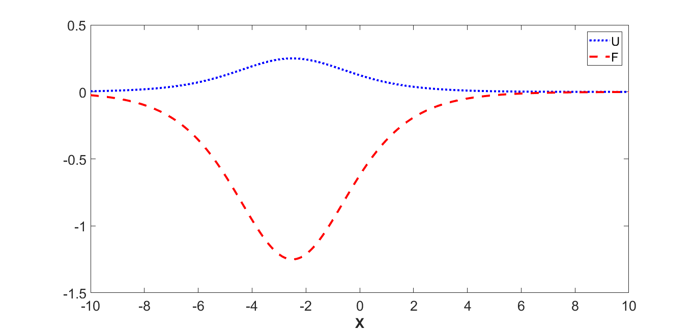
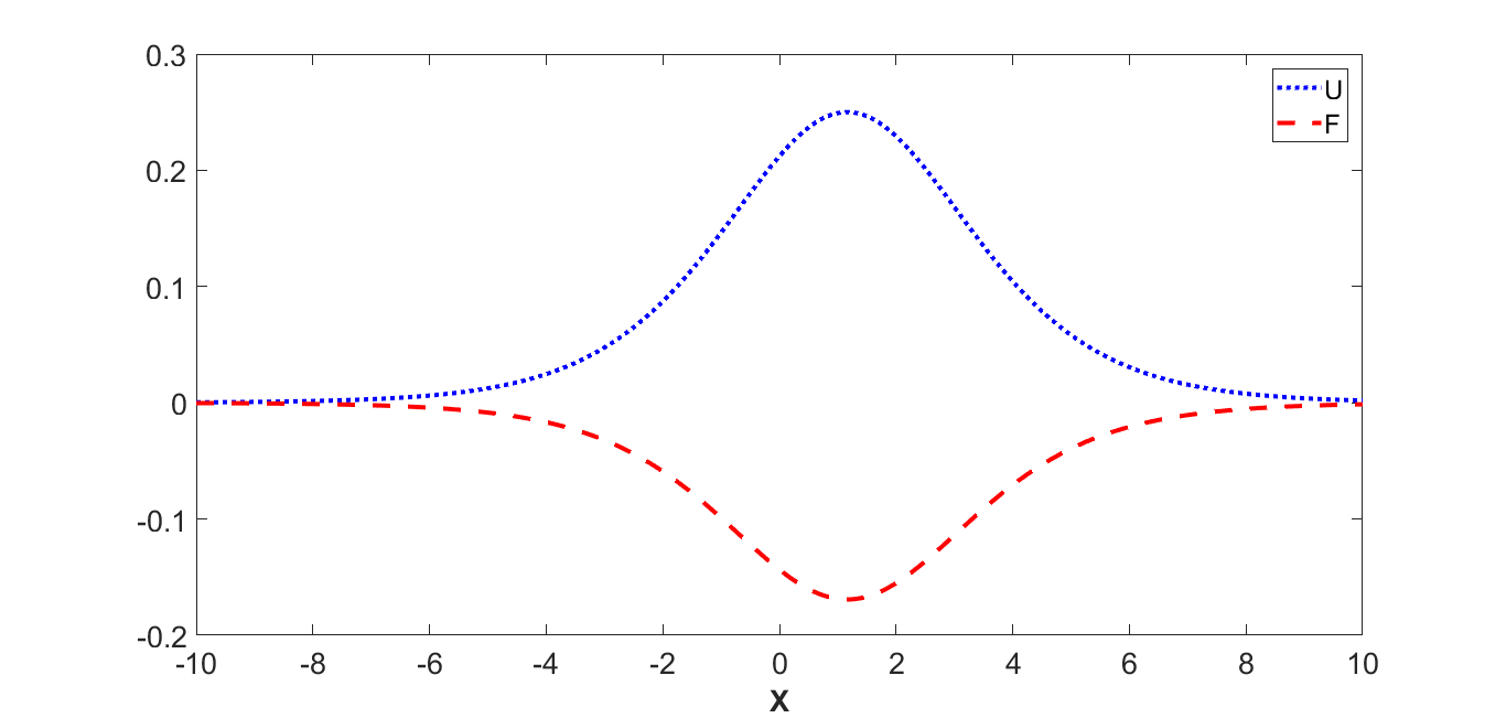
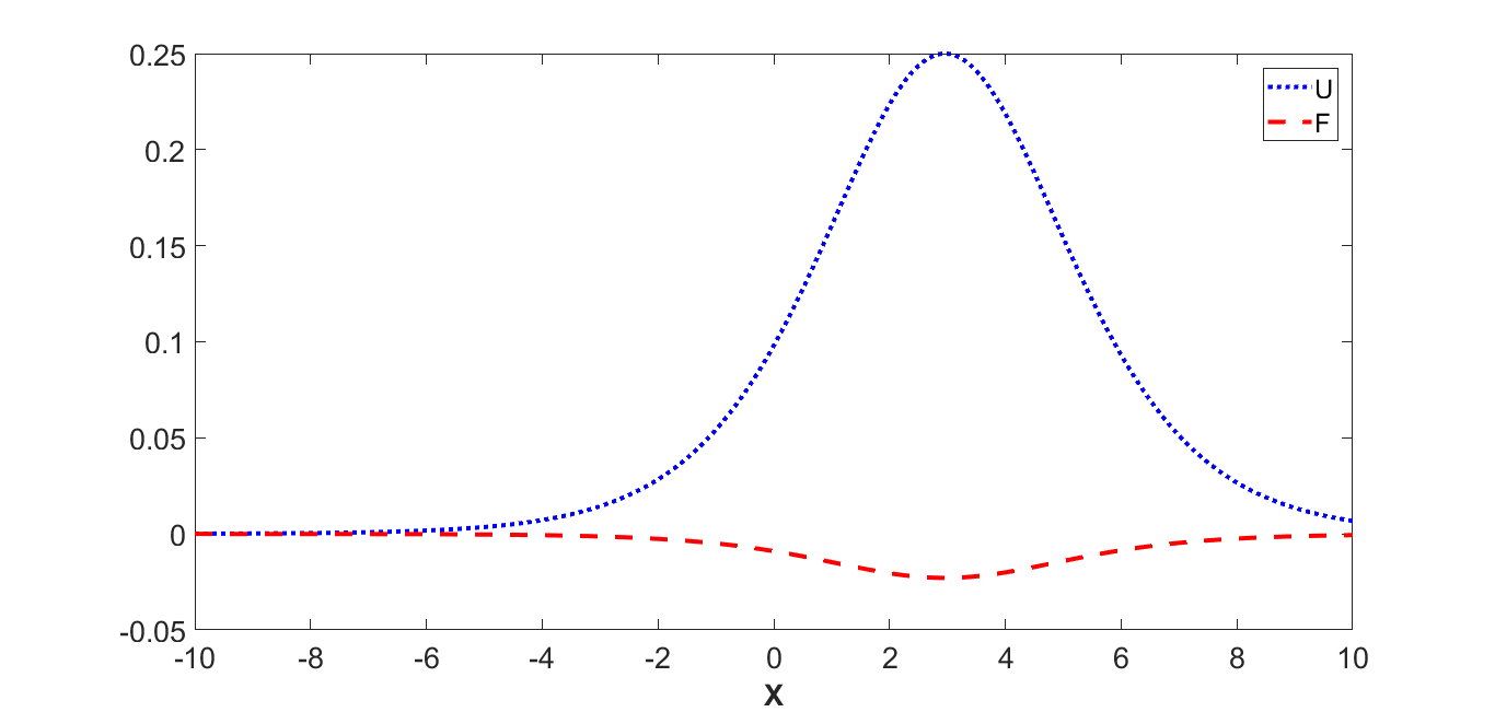
Figure 1: Plots of decelerated solitary wave solution $U$ given by equation (31) and forcing function $F$ given by equation (30) with $X$ at $Y=0$ for times $T=0$, $T=1$ and $T=2$ respectively, for the choice of $d_{1}=1.5$ and $a(T)=-5e^{-2T}$. The top, middle and bottom sub-figures in the above figure indicate the natures of $U$ and $F$ at $T=0$, $T=1$ and $T=2$ respectively, with dotted blue line and dashed red line corresponding to $U$ and $F$ respectively. The plots clearly indicate that $U$ and $F$ are pinned to each other, i.e. they move with the same velocity in spite of having different amplitudes.

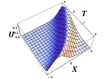
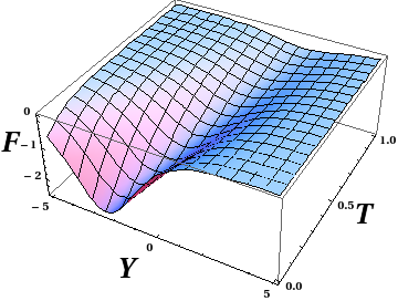
Figure 2: The above figures show 3D plots of DIAW solution $U$ and debris function $F$ given by equations (31) and (30) respectively on $X-T$ plane for $Y=0$, $a(T)=-5e^{-2T}$ and $d_{1}=1.5$. The exponential form of $a(T)$ causes the DIAW to decelerate with time; whereas its amplitude remains constant. On the other hand, both the amplitude and velocity of source debris function $F$ varies with time.

The solutions obtained so far for one solitary wave can be generalized to a $N$ solitary wave solution $U$ of Eq.(28) having time varying velocity. Similarly, the $N$ debris function $F$ that is pinned with the dust ion acoustic solitary wave also accelerates / decelerates while propagation. Using Hirota formalism Wazwaz ; BendingMukh , the two solitary wave solution $U$ of (28) can be evaluated as

$${}U=2\ [lnG]_{XX},\ G=1+\exp{(\theta_{1})}+\exp{(\theta_{2})}+a_{12}\exp{(\theta_{1}+\theta_{2})},$$

$${}a_{12}=\frac{[3k_{1}^{2}\ k_{2}^{2}\ (k_{1}-k_{2})^{2}-(k_{1}m_{2}-k_{2}m_{1})^{2}]}{[3k_{1}^{2}\ k_{2}^{2}\ (k_{1}+k_{2})^{2}-(k_{1}m_{2}-k_{2}m_{1})^{2}]},\ \theta_{i}=[k_{i}X+m_{i}Y-\frac{k_{i}^{4}+m_{i}^{2}}{k_{i}}T+\int a(T)dT]$$ (32)

for the choice of the debris function

$${}F=2a(T)\ [lnG]_{XX},\ G=1+\exp{(\theta_{1})}+\exp{(\theta_{2})}+a_{12}\exp{(\theta_{1}+\theta_{2})},$$

$${}a_{12}=\frac{[3k_{1}^{2}\ k_{2}^{2}\ (k_{1}-k_{2})^{2}-(k_{1}m_{2}-k_{2}m_{1})^{2}]}{[3k_{1}^{2}\ k_{2}^{2}\ (k_{1}+k_{2})^{2}-(k_{1}m_{2}-k_{2}m_{1})^{2}]},\ \theta_{i}=[k_{i}X+m_{i}Y-\frac{k_{i}^{4}+m_{i}^{2}}{k_{i}}T+\int a(T)dT],$$ (33)

where $k_{i},m_{i}$ are constants. Here, the amplitude of $F$ varies with time whereas that of $U$ remains constant. But both $U$ and $F$ accelerate / decelerate with the same velocity that depends on $a(T)$.

Generalizing above solutions, the accelerated $N$ solitary wave solution $U$ of (28) can be obtained as

$${}U=2\ [lnG]_{XX},$$

$${}G=\sum_{\mu=0,1,2}[\prod_{j=1}^{n}\ (\frac{\beta_{j}}{2ik_{j}})^{\mu_{j}(\mu_{j}-1)}\ (\beta_{j}\delta_{kj}+\eta_{j}^{(0)})^{\mu_{j}(2-\mu_{j})}\ \exp{(\sum_{j=1}^{n}\mu_{j}\xi_{j}+\sum_{1\leq j<l}^{n}\mu_{j}\mu_{l}A_{jl})}],$$

$${}\xi_{j}=k_{j}(\omega_{j}T+X+\int a(T)dT+p_{j}Y)+\xi_{j}^{(0)},$$

$${}\eta_{l}=\alpha_{l}T+\beta_{l}(X+\int a(T)dT)+\gamma_{l}Y+\eta_{l}^{(0)},\ \gamma_{j}=\beta_{j}p_{j}$$

$${}\exp{(A_{jl})}=\frac{(k_{j}-k_{l})^{2}-(1/3)(p_{j}-p_{l})^{2}}{(k_{j}-k_{l})^{2}-(1/3)(p_{j}-p_{l})^{2}},$$ (34)

for the choice of

$${}F=2\ a(T)\ [lnG]_{XX},$$

$${}G=\sum_{\mu=0,1,2}[\prod_{j=1}^{n}\ (\frac{\beta_{j}}{2ik_{j}})^{\mu_{j}(\mu_{j}-1)}\ (\beta_{j}\delta_{kj}+\eta_{j}^{(0)})^{\mu_{j}(2-\mu_{j})}\ \exp{(\sum_{j=1}^{n}\mu_{j}\xi_{j}+\sum_{1\leq j<l}^{n}\mu_{j}\mu_{l}A_{jl})}],$$

$${}\xi_{j}=k_{j}(\omega_{j}T+X+\int a(T)dT+p_{j}Y)+\xi_{j}^{(0)},$$

$${}\eta_{l}=\alpha_{l}T+\beta_{l}(X+\int a(T)dT)+\gamma_{l}Y+\eta_{l}^{(0)},\ \gamma_{j}=\beta_{j}p_{j}$$

$${}\exp{(A_{jl})}=\frac{(k_{j}-k_{l})^{2}-(1/3)(p_{j}-p_{l})^{2}}{(k_{j}-k_{l})^{2}-(1/3)(p_{j}-p_{l})^{2}},$$ (35)

where $k_{j},\omega_{j},p_{j},\xi_{j}^{0},\alpha_{l},\beta_{l},\gamma_{l},\eta_{l}^{(0)}$ are arbitrary real constants. The variation of the velocities of $U,F$ comes due to the presence of $a(T)$. Thus, we have obtained a family of special exact pinned solitary wave solutions for both $F$ and $U$ having accelerating / decelerating feature, that may be useful in future research on this subject.

IV Exact pinned curved solitary wave solution

In the previous section, we have found a family of exact pinned accelerated solitary wave solutions, the velocity of which changes over time instead of being constant. Such accelerated solitary waves move simultaneously with the charged debris object; hence are called pinned solitary waves. The amplitude of dust ion acoustic solitary wave remains constant whereas both the amplitude and velocity of debris function changes causing shape changing effects. Generally, in real space plasma environment, the density localization may not be always of the form of line solitons. It may bend, twist or turn during its propagation. Hence, to model such real physical phenomena, solitary wave solutions with arbitrary free functions may be useful that have such bending properties. Hence, along with arbitrary accelerated solitary waves, curved solitary waves on $x-y$ plane are also important. In this section, we will try to find such kind of exact solitary wave solutions which can bend on $x-y$ plane depending on the forcing debris function. In SenKumar , a numerical simulation for the propagation of magnetosonic wave is performed with a two dimensional circular source term. A noticeable difference from 1D simulation is observed in the shapes of wakes and precursors; which are curved in nature. This observation also strengthens the possibility of existence of curved solitary waves in experiment. There is no generalized exact solution of forced KP equation. In most of the cases, the forcing function destroys the complete integrability of the equation; hence its exact solvability is also lost. But for certain special localized forcing functions, we can get exact solutions.

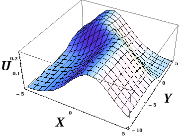
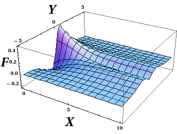
Figure 3: The above figures show 3D plots of DIAW solution $U$ and debris function $F$ given by equations (36) and (37) respectively on $X-Y$ plane at $T=0$, $c_{1}=0.5$ and $\theta_{0}=0$ for the choice of arbitrary function as : $A(Y)=\int sech{Y}dY$. It can be easily seen that both $U$ and $F$ get curved on $X-Y$ plane.

An exact pinned solitary wave solution $U$ of (28) that can bend on $X-Y$ plane is obtained in the following form

$$U=\frac{c_{1}}{2}\ Sech^{2}[\frac{\sqrt{c_{1}}}{2}\ (X+A(Y)-c_{1}T+\theta_{0})],$$ (36)

for the choice of the forcing debris function $F$ as

$${}F=A_{Y}^{2}\ \frac{c_{1}}{2}\ Sech^{2}[\frac{\sqrt{c_{1}}}{2}\ (X+A(Y)-c_{1}T+\theta_{0})]+\sqrt{c_{1}}\ A_{YY}(\ \ \tanh[\frac{\sqrt{c_{1}}}{2}\ (X+A(Y)-c_{1}T+\theta_{0})]-\ 1),\ X>0,$$

$${}F=A_{Y}^{2}\ \frac{c_{1}}{2}\ Sech^{2}[\frac{\sqrt{c_{1}}}{2}\ (X+A(Y)-c_{1}T+\theta_{0})]+\sqrt{c_{1}}\ A_{YY}(\ \ \tanh[\frac{\sqrt{c_{1}}}{2}\ (X+A(Y)-c_{1}T+\theta_{0})]+\ 1),\ X\leq 0$$ (37)

where $c_{1}$ is a constant and $A(Y)$ is an arbitrary function of Y. The function $F$ in Eq. (37) vanishes as $X\longrightarrow\pm\infty$ satisfying Poisson’s equation (4) as discussed before. There might be other choices of $F$ to get exact curved solitary wave solution $U$ of (28), but we consider (37) as the first example of $F$ to explore the situation. The nonlinear function $A(Y)$ makes the solitary wave to bend in $X-Y$ plane. Both the solutions $U$ and $F$ given by equation (36) and (37) are pinned solutions, like the solutions discussed in previous section. As we have shown in the previous section, the pinned nature can be understood by plotting both $U,F$ with $X$ at different times. The 3D plots of both $U$ and $F$ given by the above equations (36) and (37) for a given choice of $A(Y)$ are provided in Figure-3. Thus we have provided an exact pinned curved solution $U$ for Eq. (28) for a specific choice of the localized function $F$. The solution may be used for modeling the twist or turn of the solitary waves during its motion in real experiments. Though there may be more general numerical or approximate solutions, but the exact form of this curved solution makes it important in this field.

V Results and Discussions

A few specific points of this work, that need to be discussed, are stated below.

1. In this work, we have derived few (2+1) dimensional exact dust ion acoustic solitary wave solutions for choice of specific localized debris functions. The constant amplitude exact solitary waves $U$ may accelerate or bend on $X-T$ and $X-Y$ planes respectively due to specific choices of the forcing functions as discussed in section-III and section-IV.

2. We can see that the coefficient of each term in equation (26) depends on $v_{p}$ which depends on $\alpha$ via equation (23), i.e,

   $$v_{p}=\frac{1}{\sqrt{1-\alpha}},\ \alpha=Z_{d}\frac{n_{d0}}{n_{i0}}.$$ (38)

   Hence, we can see that $\alpha$ must be $<1$ for a real $v_{p}$. The variation of phase velocity $v_{p}$ with parameter $\alpha$ is plotted in Figure-4, where we see that $v_{p}$ increases with $\alpha$. For ion acoustic wave, we can evaluate $v_{p}$ to be = 1. The static dust grains increase the phase velocity by a factor $\frac{1}{\sqrt{1-\alpha}}.$

   

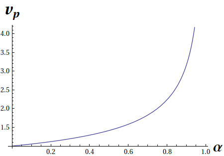
   Figure 4: Variation of phase velocity $v_{p}$ with $\alpha$.

3. The solitary wave gets accelerated / decelerated due to presence of nonlinear function $a(T)$. Obviously, for $a(T)=$ constant, we get the standard line solitary waves having constant velocity. The acceleration of the solitary wave is shown by the contour plots in Figure-5 and Figure-6.

   

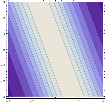
   Figure 5: The contour plot of the DIAW solution $U$ (31) in $X-T$ plane for $Y=0$, $a(T)=2,d_{1}=1.5$. We can see that the peak of the solitary wave $U$ moves along a straight line in $X-T$ plane for $a(T)=$ constant, thus showing the usual line solitary waves.

   

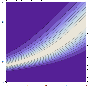
   Figure 6: The contour plot of the DIAW solution $U$ (31) in $X-T$ plane for $Y=0$, $a(T)=-5e^{-2T},d_{1}=2$. We can see that the peak of the solitary wave $U$ moves along a curved path in $X-T$ plane for the exponential form of $a(T)$.

4. The exact accelerated solitary wave solution (31), which we have found, can be expressed in old variables as

   $$n_{1}=\frac{3B(d_{1}-1)}{A}\ sech^{2}[\frac{\sqrt{d_{1}-1}}{2}\{\xi+\sqrt{(B/C)}\eta-d_{1}B\tau-(\frac{60B^{3}}{DA})\int\exp{(-2B\tau)}d\tau\}],$$ (39)

   where the coefficients $A,B,C$ are given as

   $${}A=\frac{v_{p}(3-v_{p}^{2})}{2},\ B=\frac{v_{p}^{3}}{2},\ C=D=\frac{v_{p}}{2},$$ (40)

   for $a(T)=-5e^{-2T}$. The variation of the DIAW $n_{1}$ in (39) with $\alpha$ at the center $\xi=\eta=0$ at $\tau=1$ is shown in Figure-7.

   

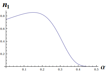
   Figure 7: The variation of the DIAW $n_{1}$ in (39) with $\alpha$ at the center $\xi=\eta=0$ at $\tau=1$ for $d_{1}$ = 1.5.

5. In this work, we have also derived an exact curved solitary wave solution for a special localized debris function. The exact solitary wave solution can bend on $x-y$ plane depending on the forcing function. In SenKumar , a two dimensional circular source term is considered in their numerical simulation for the propagation of magnetosonic wave. The noticeable difference from the 1D simulation is in the shapes of wakes and precursors which are curved in nature. This observation also strengthens the possibility of observing the exact curved solitary wave solution (36) in experimental scenario. It should be noted that curvature of the solution (36) occurs due to presence of nonlinear function $A(Y)$ in the argument of the solution (36). Now it is required to determine how much curvature is taking place by varying $A(Y)$ i.e, what the condition is for larger bending. For static case ($T=0$), the locus of the maximum amplitude of the curved solitary wave solution (36) is of the form:

   $$\frac{\sqrt{c_{1}}}{2}\ (X+A(Y)+\theta_{0})=0.$$ (41)

   Now taking derivative w.r.to $Y$ twice in the above equation (41) we get,

   $$\frac{dS}{dY}=-A_{YY},$$ (42)

   where the slope is defined as: $S=\frac{dX}{dY}.$ We see from (42) that for higher value of RHS, rate of variation of the slope $S$ will be higher. Hence in that case, the slope of the maximum amplitude curve will vary large for traversing unit distance in $Y$. Larger rate of variation of slope $S$ describes larger bending. Hence, for large bending of solitary waves to take place, the double derivative of $A(Y)$ must also be high. This is explained clearly by the contour plot in Figure-8.

   

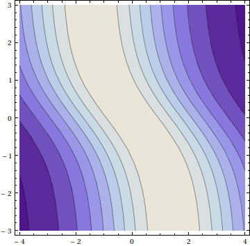
   Figure 8: Contour plot of curved dust ion acoustic solitary wave solution $U$ given by equation (36) on $X-Y$ plane at $T=0$ for $c_{1}=0.5$, $\theta_{0}=0$ and $A(Y)=\int sech{Y}dY$. The figure shows that DIAW solution $U$ bends on $X-Y$ plane due to the function $A(Y)$.

6. Similar to the exact solutions obtained in Sen , we derive few intricate exact solitary wave solutions. The only difference is the solutions derived in Sen are line solitary waves whereas solutions derived in the present work are accelerated and curved solitary waves. Basically we have investigated few specific forms of $F$ for which we get exact solitary wave solutions for $U$ having bending features. The velocity profiles for both $U$ and $F$ are obtained to be identical. For other general choice of $F$, perturbative or numerical solutions need to be obtained

VI Concluding remarks

In this work, we have considered the low temperature and low density plasma in the LEO region in presence of localized charged space debris particles. The dynamics of (2+1) dimensional nonlinear dust ion acoustic waves induced in the system is found to be governed by a forced KP-II equation, where the forcing term depends on the charged space debris function. We have found some exact curved solitary wave solutions for the DIAW that can bend on $x-t$ and $x-y$ planes respectively. A family of exact pinned accelerated solitary wave solutions (30) - (35) have been derived. The velocity of the solutions changes over time whereas the amplitude remains constant. The solutions contain an arbitrary time dependent function $a(T)$ that can be chosen accordingly for modeling different types of dynamics of the solutions. Also, a special exact solitary wave solution (36) has been derived for a special debris function (37) that gets curved on $x-y$ plane; where its curvature depends on the nature of the forcing debris function. The solution also contain an arbitrary function $A(Y)$. For different choices of $A(Y),$ we would get different kinds of bending of the solitary wave. Thus, the exact solutions of this work may be interesting to the nonlinear dynamics community and useful for different practical applications.

VII acknowledgements

Siba Prasad Acharya acknowledges Department of Atomic Energy (DAE) of Government of India for financial help during this work through institute fellowship scheme. Abhik Mukherjee would like to acknowledge Indian Statistical Institute, Kolkata for the financial support during the research work. Abhik Mukherjee is indebted to Ms. Krishna Kar for the scintillating discussions and unconditional support during the progress of the work. The authors are immensely grateful to the anonymous reviewers for their fruitful suggestions to improvise this work.

VIII References

References

- (1) Space Plasma Physics: The Study of Solar-System Plasmas, National Research Council (1978) Washington, DC: The National Academies Press.
- (2) H. Klinkrad, Space Debris Models and Risk Analysis, Springer Praxis Books, Praxis Publishing Ltd, Chichester, UK (2006).
- (3) J. C. Sampaio, E. Wnuk, R. Vilhena de Moraes, and S. S. Fernandes, Resonant Orbital Dynamics in LEO Region: Space Debris in Focus, Mathematical Problems in Engineering, Volume 2014, Article ID 929810.
- (4) I. Kulikov and M. Zak, Detection of Moving Targets Using Soliton Resonance Effect, Advances in Remote Sensing, 1 (2012) 58.
- (5) A. Sen, S. Tiwari, S. Mishra and P. Kaw, Nonlinear wave excitations by orbiting charged space debris objects, Advances in Space Research, 56 (2015) 429.
- (6) S. P. Acharya, A. Mukherjee, and M. S. Janaki, Accelerated magnetosonic lump wave solutions by orbiting charged space debris, Nonlinear Dyn (2021).
- (7) M. Horányi, Charged dust dynamics in the solar system, Annual Review of Astronomy and Astrophysics, 34 (1996) 383-418.
- (8) Technical Report on Space Debris, United Nations Publication, ISBN 92-1-100813-1, New York, 1999.
- (9) S. K. Tiwari and A. Sen, Wakes and precursor soliton excitations by a moving charged object in a plasma, Phys. Plasmas 23 (2016) 022301.
- (10) S. K. Tiwari and A. Sen, Fore-wake excitations from moving charged objects in a complex plasma, Phys. Plasmas 23 (2016) 100705.
- (11) S. Jaiswal, P. Bandyopadhyay, and A. Sen, Experimental observation of precursor solitons in a flowing complex plasma, Physical Review E 93 (2016), 041201(R).
- (12) G. Arora, P. Bandyopadhyay, M. G. Hariprasad and A. Sen, Effect of size and shape of a moving charged object on the propagation characteristics of precursor solitons, Phys. Plasmas 26 (2019), 093701.
- (13) P. K. Shukla and V. P. Silint, Dust ion-acoustic wave, Physica Scripta. 45 (1992) 508.
- (14) P. K. Shukla and A. A. Mamun, Introduction to Dusty Plasma Physics, IOP Publishing Ltd, Plasma Phys. Control. Fusion 44 395 (2002).
- (15) S. S. Duha, M. G. M. Anowar, and A. A. Mamun, Dust ion-acoustic solitary and shock waves due to dust charge fluctuation with vortexlike electrons, Physics of Plasmas 17, 103711 (2010).
- (16) A. A. Mamun and S. Islam, Nonplanar dust-ion-acoustic double layers in a dusty nonthermal plasma, J. Geophys. Res. 116, A12323 (2011).
- (17) S. I. Popel and M. Y. Yu, Ion Acoustic Solitons in Impurity-Containing Plasmas, Contrib. Plasma Phys. 35, 103 (1995).
- (18) G. C. Das, J. Sarma, and R. Roychoudhury, Some aspects of shock-like nonlinear acoustic waves in magnetized dusty plasma, Phys. Plasmas 8, 74 (2001).
- (19) M. G. M Anowar and A. A. Mamun, Multidimensional Instability of Dust-Ion-Acoustic Solitary Waves IEEE Trans. Plasma Sci. 36, 2867 (2008).
- (20) A. A. Mamun, R. A. Cairns, and P. K. Shukla, Dust negative ion acoustic shock waves in a dusty multi-ion plasma, Phys. Lett. A 373, 2355 (2009).
- (21) Robert L. Merlino, and John A. Goree, Dusty Plasmas in the Laboratory, Industry, and Space, Physics Today 57, 7, 32 (2004).
- (22) O. Rahman and A. A. Mamun, Dust-ion-acoustic solitary waves in dusty plasma with arbitrarily charged dust and vortex-like electron distribution, Physics of Plasmas 18, 083703 (2011).
- (23) S. Yasmin, M. Asaduzzaman, and A. A. Mamun, Evolution of higher order nonlinear equation for the dust ion-acoustic waves in nonextensive plasma, Phys. Plasmas 19, 103703 (2012).
- (24) F. Verheest, T. Cattaert, and M. A. Hellberg, Ion- and dust-acoustic solitons in dusty plasmas: Existence conditions for positive and negative potential solutions, Phys. Plasmas 12, 082308 (2005).
- (25) A. A. Mamun, P. K. Shukla, and B. Eliasson, Solitary waves and double layers in a dusty electronegative plasma, Phys. Rev. E 80, 046406 (2009).
- (26) F. Verheest, M. A. Hellberg, and I. Kourakis, Dust-ion-acoustic supersolitons in dusty plasmas with nonthermal electrons, Physical Review E 87, 043107 (2013).
- (27) A. A. Mamun and P. K. Shukla, Cylindrical and spherical dust ion–acoustic solitary waves, Physics of Plasmas 9, 1468 (2002).
- (28) A. A. Mamun, Effects of adiabaticity of electrons and ions on dust-ion-acoustic solitary waves, Physics Letters A 372 (2008) 1490–1493.
- (29) A. A. Mamun, and P. K. Shukla, Effects of nonthermal distribution of electrons and polarity of net dust-charge number density on nonplanar dust-ion-acoustic solitary waves, Physical Review E 80, 037401 (2009).
- (30) R. Bharuthram, and P. K. Shukla, Large amplitude ion-acoustic solitons in a dusty plasma, Planet. Space Sci. 40, 7, 973-977 (1992).
- (31) Alexis S. Truitt, and Christine M. Hartzell, Simulating Plasma Solitons from Orbital Debris Using the Forced Korteweg–de Vries Equation, Journal of Spacecrafts and Rockets 57 (2020) 5.
- (32) Alexis S. Truitt, and Christine M. Hartzell, Three-Dimensional Kadomtsev–Petviashvili Damped Forced Ion Acoustic Solitary Waves from Orbital Debris, Journal of Spacecrafts and Rockets 58 (2021) 3.
- (33) Alexis S. Truitt, and Christine M. Hartzell, Simulating Damped Ion Acoustic Solitary Waves from Orbital Debris, Journal of Spacecrafts and Rockets 57 (2020) 5.
- (34) R. Ali, A. Saha and P. Chatterjee, Analytical electron acoustic solitary wave solution for the forced KdV equation in superthermal plasmas, Physics of Plasmas, 24 (2017) 122106.
- (35) P. Chatterjee, R. Ali and A. Saha, Analytical Solitary Wave Solution of the Dust Ion Acoustic Waves for the Damped Forced Korteweg–de Vries Equation in Superthermal Plasmas, Zeitschrift fur Naturforschung A, 73 (2018) 151.
- (36) H. Zhen, B. Tian, H. Zhong, W. Sun and M. Li, Dynamics of the Zakharov-Kuznetsov-Burgers equations in dusty plasmas, Physics of Plasmas, 20 (2013) 082311.
- (37) L. Mandi, A. Saha and P. Chatterjee, Dynamics of ion-acoustic waves in Thomas-Fermi plasmas with source term, Advances in Space Research, 64 (2019) 427-435.
- (38) A. Mukherjee, S. P. Acharya and M. S. Janaki, Dynamical study of nonlinear ion acoustic waves in presence of charged space debris at Low Earth Orbital (LEO) plasma region, Astrophys Space Sci, 366 (2021), 7.
- (39) A. N. Dev et. al, Kadomtsev—Petviashvili (KP) Burgers Equation in Dusty Negative Ion Plasmas: Evolution of Dust-Ion Acoustic Shocks, Commun. Theor. Phys. 62 (2014) 875.
- (40) H. U. Rehman, Kadomtsev–Petviashvili equation for dust ion-acoustic solitons in pair-ion plasmas, Chin. Phys. B 22 (2013) 035202.
- (41) O. Rahman and Md. M. Haider, Modified Korteweg-de Vries (mK-dV) Equation Describing Dust-ion-acoustic Solitary Waves in an Unmagnetized Dusty Plasma with Trapped Negative Ions, Advances in Astrophysics. 1 (2016) 161.
- (42) A. Kumar and A. Sen, Precursor magneto-sonic solitons in a plasma from a moving charge bunch, New J. Phys. 22 (2020) 073057.
- (43) R. A. Kraenkel, J. G. Pereira and M. A. Manna, The reductive perturbation method and the Korteweg-de Vries hierarchy, Acta Appl Math 39 (1995) 389–403.
- (44) A. Kundu, Journal of Physics A: Mathematical and Theoretical, Exact accelerating solitons in nonholonomic deformation of the KdV equation with a two-fold integrable hierarchy, 41 (2008) 495201.
- (45) A. Kundu, Journal of Physics A: Mathematical and Theoretical, Nonholonomic deformation of KdV and mKdV equations and their symmetries, hierarchies and integrability, 42 (2009), 115213.
- (46) R. Grimshaw, M. Maleewong, and J. Asavanant, Stability of gravity-capillary waves generated by a moving pressure disturbance in water of finite depth, Physics of Fluids 21 (2009) 8 82–101.
- (47) A. M. Wazwaz, Multiple-soliton solutions for the KP equation by Hirota’s bilinear method and by the tanh–coth method, Applied Mathematics and Computation. 190 (2007) 633.
- (48) A. Mukherjee, M. S. Janaki and A. Kundu, Bending of solitons in weak and slowly varying inhomogeneous plasma, Phys. Plasmas. 22 (2015) 122114.