Gravitational Wave Background Search by Correlating Multiple Triangular Detectors
in the mHz Band

Abstract

With the recent strong developments of TianQin and Taiji, we now have an increasing chance to make a correlation analysis in the mHz band by operating them together with LISA. Assuming two LISA-like triangular detectors at general geometrical configurations, we develop a simple formulation to evaluate the network sensitivity to an isotropic gravitational wave background. In our formulation, we fully use the symmetry of data channels within each triangular detector and provide tractable expressions without directly employing cumbersome detector tensors. We concretely evaluate the expected network sensitivities for various potential detector combinations, including the LISA-TianQin pair.

I Introduction

A cosmological gravitational wave background is an important observational target for studying our universe Romano:2016dpx ; Caprini:2018mtu . It is expected to have a nearly isotropic intensity pattern. We can statistically amplify the background signal by correlating noise independent detectors Christensen:1992wi ; Flanagan:1993ix ; Allen:1997ad (see also Hellings:1983fr ). Around 10-1000 Hz, the observational constrains have been significantly improved with the suppression of instrumental noises of ground based detectors. The latest result by the LIGO-Virgo collaboration is $\Omega_{GW}<6.0\times 10^{-8}$ LIGOScientific:2019vic . On another front, quite recently, the nano-Hertz band is fueled by a report from NANOGrav Arzoumanian:2020vkk .

LISA has been the leading project for gravitational wave observation around $10^{-4}$-0.1Hz lisa0 ; lisa . It is scheduled to be launched around 2035. From its triangular detector, we can take three noise independent data channels Prince:2002hp . Unfortunately, due to symmetric cancellations, the correlations between the noise independent data channels are known to be insensitive to the monopole pattern of a background Romano:2016dpx (see also Tinto:2001ii ; Hogan:2001jn ; Adams:2010vc for a different approach with Sagnac-type data streams). But, recently, the situations have been changed rapidly with the strong developments of two Chinese projects; TianQin Luo:2015ght and Taiji taiji (see Fig.1 for their noise spectra). In this context, the author studied the prospects specifically for the LISA-Taiji network Seto:2020zxw (see also Cornish:2001bb ; 1821247 ; Ruan:2019tje ). He pointed out two important symmetries inherent to the network. The first one is the geometric symmetry about the relative configuration of LISA and Taiji. We can take a virtual sphere that simultaneously contacts with the two detector planes. The second symmetry is about the combinations of data channels within each triangular detector (related to the insensitivity to the monopole pattern mentioned above). It was shown that, as a result of the two symmetries, the LISA-Taiji network allows us to make a simple parity decomposition for an isotropic gravitational wave background Seto:2020zxw .

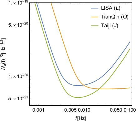
Figure 1: The instrumental noise spectra for the planned triangular detectors. Each curve is given for a single ($A$ and $E$) data channel without angular averages.

In this paper, we study general network configurations for two LISA-like triangular detectors. Now, in contrast to the LISA-Taiji network, the first geometrical symmetry mentioned above is no longer available. But we can still exploit the second symmetry about the internal data channels. Indeed, taking the advantage of the second one, we only need three angular parameters for characterizing the homothetic structure of the network geometry. This enables us to develop a simple formulation for evaluating the network sensitivities to an isotropic background. In this formulation, without directly handling cumbersome detector tensors, we calculate some polynomials given by the cosines of the three angular parameters. Using our formulation, we concretely evaluate the sensitivities for networks formed by pairing LISA, TianQin, Taiji and their variations.

This paper is organized as follows. In Sec.II, we review the basic aspects of the correlation analysis. In Sec.III, we study the networks composed by two LISA-like triangular detectors and develop a new formulation, fully using the symmetry of their data combinations. In Sec.IV, we explain how our analytical expressions are simplified for networks with high geometrical symmetries. In Sec.V, we apply our formulation to the mHz-band networks formed by LISA, TianQin, Taiji and their variations. In Sec.VI, we numerically evaluate the signal-to-noise ratios for potential networks.

II correlation analysis

In this section, we make a brief discussion on the correlation analysis for detecting an isotropic gravitational wave background (see Romano:2016dpx ; Flanagan:1993ix ; Allen:1997ad for detail).

II.1 background signal

We can expand the metric perturbation at a position ${x}$ induced by a gravitational wave background as

$${\mbox{\boldmath${h}$}}(f,{\mbox{\boldmath${x}$}})=\sum_{P={+,\times}}\int d\mbox{\boldmath${n}$}\,h(f\mbox{\boldmath${n}$},P){\mbox{\boldmath${e}$}}_{p}\,e^{-2\pi if\mbox{\boldmath${n}$}\cdot{\mbox{\boldmath${x}$}}/c}.$$ (1)

Here the unit vector ${n}$ shows the propagation direction of a wave, and the factor $h(f\mbox{\boldmath${n}$},P)$ is the mode coefficient. The polarization tensors ${\mbox{\boldmath${e}$}}_{P},(P=+,\times)$ are given by the orthonormal transverse vectors $\mbox{\boldmath${l}$}_{1}$ and $\mbox{\boldmath${l}$}_{2}$ as

$${\mbox{\boldmath${e}$}}_{+} = \mbox{\boldmath${l}$}_{1}\otimes\mbox{\boldmath${l}$}_{1}-\mbox{\boldmath${l}$}_{2}\otimes\mbox{\boldmath${l}$}_{2}$$ (2)

$${\mbox{\boldmath${e}$}}_{\times} = \mbox{\boldmath${l}$}_{1}\otimes\mbox{\boldmath${l}$}_{2}+\mbox{\boldmath${l}$}_{2}\otimes\mbox{\boldmath${l}$}_{1}.$$ (3)

In this paper, as Eq.(1), we mainly use quantities in the Fourier space rather than the time space.

We assume that the gravitational wave background is isotropic, stationary and randomly polarized. Then, the covariance of the mode coefficients is written by

$$\left\langle h(f\mbox{\boldmath${n}$},P)h(f^{\prime}{}\mbox{\boldmath${n}$}^{\prime}{},P^{\prime}{})^{*}\right\rangle=\delta(f\mbox{\boldmath${n}$}-f^{\prime}{}\mbox{\boldmath${n}$}^{\prime}{})\delta_{P,P^{\prime}{}}S_{h}(f).$$ (4)

In general relativity, the strain spectrum $S_{h}(f)$ is given by the normalized energy density $\Omega_{GW}(f)$ as

$$S_{h}(f)=\frac{3H_{0}^{2}}{32\pi^{3}}\Omega_{GW}(f)$$ (5)

with the Hubble parameter $H_{0}$ that is fixed at $70{\rm km^{1}s^{-1}Mpc^{-1}}$ below.

II.2 cross correlation

Next we consider an equal-arm L-shaped interferometer $a$ at a position ${\mbox{\boldmath${x}$}}_{a}$, and discuss its response $h_{a}(f)$ to the background. In the low frequency approximation, the response is characterized by the detector tensor

$$\mbox{\boldmath${D}$}_{a}=({\mbox{\boldmath${u}$}}\otimes{\mbox{\boldmath${u}$}}-{\mbox{\boldmath${v}$}}\otimes{\mbox{\boldmath${v}$}})/2$$ (6)

with the unit vectors ${u}$ and ${v}$ representing the two arm directions (${\mbox{\boldmath${u}$}}\cdot{\mbox{\boldmath${v}$}}=0$). Then, the interferometric response to the background is given by

$$h_{a}(f)=\sum_{P={+,\times}}\int d\mbox{\boldmath${n}$}\,h(f\mbox{\boldmath${n}$},P)\,e^{-2\pi if\mbox{\boldmath${n}$}\cdot{\mbox{\boldmath${x}$}}_{a}/c}F_{a}^{P}(\mbox{\boldmath${n}$})$$ (7)

with the beam pattern function $F_{a}^{P}(\mbox{\boldmath${n}$})=(\mbox{\boldmath${D}$}_{a}:{\mbox{\boldmath${e}$}}_{P})$. In reality, the data stream $s_{a}(f)$ of the detector $a$ contains not only the signal $h_{a}(f)$ but also various noises $n_{a}(f)$. Therefore, we put

$$s_{a}(f)=h_{a}(f)+n_{a}(f).$$ (8)

The noise spectrum $N_{a}(f)$ is defined by

$$\left\langle n_{a}(f)n_{a}(f^{\prime}{})^{*}\right\rangle=N_{a}(f)\delta(f-f^{\prime}{}).$$ (9)

The correlation analysis is an efficient approach to detect a weak background signal dominated by the noise $|h_{a}(f)|\ll|n_{a}(f)|$. The expectation value of the correlation product of two noise-independent detectors $a$ and $b$ is given by

$$\left\langle s_{a}(f)s_{b}(f^{\prime}{})^{*}\right\rangle = \left\langle h_{a}(f)h_{b}(f^{\prime}{})^{*}\right\rangle$$ (10)

$$= \frac{8\pi}{5}\delta(f-f^{\prime}{})\gamma_{ab}(f)S_{h}(f).$$ (11)

Here $\gamma_{ab}(f)$ is the overlap reduction function. From Eqs.(4) and (7), we have Flanagan:1993ix ; Allen:1997ad

$$\gamma_{ab}(f)=\frac{5}{8\pi}\sum_{P=+,\times}\int d\mbox{\boldmath${n}$}F_{a}^{P}(\mbox{\boldmath${n}$})F_{b}^{P}(\mbox{\boldmath${n}$})e^{2\pi if\mbox{\boldmath${n}$}\cdot({\mbox{\boldmath${x}$}}_{b}-{\mbox{\boldmath${x}$}}_{a})}.$$ (12)

Considering the diagonal structure in Eq.(11), we take the product of the data at same frequencies $f=f^{\prime}{}$. The fluctuation around the expectation value (11) is assumed to be dominated by the noises $n_{a}(f)n_{b}(f)^{*}$. In order to statistically suppress the noises, we take a summation of a large number of Fourier bins with the frequency interval $T_{\rm obs}^{-1}$ ($T_{\rm obs}$: observation period). If we take the integration range $f\in[f_{\rm min},f_{\rm max}]$, the signal-to-noise ratio is given by Flanagan:1993ix ; Allen:1997ad

$$SNR^{2} = 2\left(\frac{3H_{0}^{2}}{10\pi^{2}}\right)^{2}T_{\rm obs}$$ (13)

$$\times\left[\int_{f_{\rm min}}^{f_{\rm max}}df\frac{\Omega_{\rm GW}(f)^{2}}{f^{6}}\frac{\gamma_{ab}(f)^{2}}{N_{a}(f)N_{b}(f)}\right].$$

When we have more than one pair of noise-independent interferometers, the element $\gamma_{ab}(f)^{2}/(N_{a}(f)N_{b}(f))$ should be replaced by the summation of the corresponding combinations.

II.3 overlap reduction function

In Eq.(12), we defined the overlap reduction function $\gamma_{ab}(f)$. Here we provide its tensorial expression that will be extensively used in the next section.

Let us consider two L-shaped interferometers $a$ and $b$ separated at

$${\mbox{\boldmath${x}$}}_{b}-{\mbox{\boldmath${x}$}}_{a}=d\mbox{\boldmath${m}$}$$ (14)

with the distance $d=|{\mbox{\boldmath${x}$}}_{a}-{\mbox{\boldmath${x}$}}_{b}|$ and the normalization $|\mbox{\boldmath${m}$}|=1$. Then, in the low frequency approximation, the overlap reduction can be formally expressed as

$$\gamma_{ab}(f)=\Gamma_{ijkl}D_{a,ij}D_{b,kl}$$ (15)

with the two detector tensors $D_{a,ij}$ and $D_{b,ij}$ Flanagan:1993ix ; Allen:1997ad . The tensor $\Gamma_{ijkl}$ is written by the Kronecker’s delta and the unit vector ${m}$ as

$$\Gamma_{ijkl}(y) = b_{0}(y)\delta_{ik}\delta_{jk}+b_{1}(y)\delta_{ik}m_{j}m_{l}$$ (16)

$$+b_{2}(y)m_{i}m_{j}m_{k}m_{l}.$$

The coefficients $b_{0}$, $b_{1}$ and $b_{2}$ are given by the spherical Bessel functions $j_{l}=j_{l}(y)$ with the argument $y=2\pi fd/c$ as

$$b_{0}(y) = 2\left(j_{0}-\frac{10}{7}j_{2}+\frac{1}{14}j_{4}\right)$$ (17)

$$b_{1}(y) = 4\left(\frac{15}{7}j_{2}-\frac{5}{14}j_{4}\right)$$ (18)

$$b_{2}(y) = \frac{5}{2}j_{4}.$$ (19)

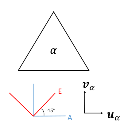
Figure 2: The geometry of the two effective L-shaped interferometers for the $A$ and $E$ channels generated from a single triangle unit $\alpha$. Their detector tensors $\mbox{\boldmath${D}$}_{A}$ and $\mbox{\boldmath${D}$}_{E}$ are characterized by the unit vectors ${u}$ and ${v}$ as in Eqs.(20) and (21). These detector tensors are attached to the triangle that spins as a result of differential orbital motions.

III triangular detectors

In this section, based on the results presented in the previous section, we study the correlation analysis specifically for two LISA-like triangular interferometers. We use the labels $\alpha$ and $\beta$ to specify the triangular units.

III.1 A and E channels

First, we discuss data streams available from a single LISA-like triangular unit $\alpha$. We can, in principle, make three interferometers symmetrically at the three vertexes. However, these data streams have correlated noises. Using the symmetry of the system, we can easily compose three data channels $A,E$ and $T$ with no correlated noises Prince:2002hp . The $T$ channel has a negligible strain sensitivity at the frequency regime relevant for our study, and we thus deal with the $A$ and $E$ channels below. They can be effectively regarded as two L-shaped interferometers with the offset angle $45^{\circ}$ (see Fig.2).

Using the orthonormal unit vectors $({\mbox{\boldmath${u}$}}_{\alpha},{\mbox{\boldmath${v}$}}_{\alpha})$ attached to the triangle $\alpha$, the detector tensor for the $A$ channel is given by

$$\mbox{\boldmath${D}$}_{A}=({\mbox{\boldmath${u}$}}_{\alpha}\otimes{\mbox{\boldmath${u}$}}_{\alpha}-{\mbox{\boldmath${v}$}}_{\alpha}\otimes{\mbox{\boldmath${v}$}}_{\alpha})/2.$$ (20)

The arm directions of the $E$ channel are given by $({\mbox{\boldmath${u}$}}_{\alpha}\pm{\mbox{\boldmath${v}$}}_{\alpha})/\sqrt{2}$, and we obtain

$$\mbox{\boldmath${D}$}_{E}=({\mbox{\boldmath${u}$}}_{\alpha}\otimes{\mbox{\boldmath${v}$}}_{\alpha}+{\mbox{\boldmath${v}$}}_{\alpha}\otimes{\mbox{\boldmath${u}$}}_{\alpha})/2.$$ (21)

With the low frequency approximation, we can readily confirm $\gamma_{AE}\propto(\mbox{\boldmath${D}$}_{A}:\mbox{\boldmath${D}$}_{E})=0$. In fact, due to the symmetry of the system, the $AE$ correlation is insensitive to an isotropic background even without the low frequency approximation.

For the noise spectra of the $A$ and $E$ channels, we have

$$\left\langle n_{A}(f)n_{A}(f^{\prime}{})^{*}\right\rangle=\left\langle n_{E}(f)n_{E}(f^{\prime}{})^{*}\right\rangle=N_{\alpha}(f)\delta(f-f^{\prime}{})$$ (22)

with no correlation

$$\left\langle n_{A}(f)n_{E}(f^{\prime}{})^{*}\right\rangle=0.$$ (23)

III.2 total SNR

Next we study correlation analysis with two triangular detectors $\alpha$ and $\beta$. Similar to the triangle $\alpha$ discussed in the previous section, we take two noise independent data streams $(A^{\prime}{},E^{\prime}{})$ from the second triangle $\beta$, and put their noise spectra by $N_{\beta}(f)$. Throughout this paper we assume that two triangles have no noise correlation.

In total, we have four data pairs $AA^{\prime}{},AE^{\prime}{},EA^{\prime}{}$ and $EE^{\prime}{}$. The total signal-to-noise ratio is given by

$$SNR_{\alpha\beta}^{2}=\left(\frac{3H_{0}^{2}}{10\pi^{2}}\right)^{2}T_{\rm obs}\left[2\int_{f_{\rm min}}^{f_{\rm max}}df\frac{\Omega_{\rm GW}(f)^{2}Y_{\alpha\beta}(f)}{f^{6}N_{\alpha}(f)N_{\beta}(f)}\right]$$ (24)

where we defined the function $Y_{\alpha\beta}(f)$ by

$$Y_{\alpha\beta}(f)\equiv\gamma_{AA^{\prime}{}}^{2}+\gamma_{AE^{\prime}{}}^{2}+\gamma_{EA^{\prime}{}}^{2}+\gamma_{EE^{\prime}{}}^{2},$$ (25)

using the four overlap reduction functions. This function $Y_{\alpha\beta}(f)$ plays a central role in the rest of this paper. We call it the total response function.

Using Eqs.(15)-(19), we can formally expand

$$Y_{\alpha\beta}=~{}\sum_{i=0}^{2}\sum_{j=0}^{2}b_{i}(y)b_{j}(y)X_{ij}.$$ (26)

Here $X_{ij}(=X_{ij})$ are given by the detector tensors $D_{a,ij}$ and the unit directional vector $m_{i}$. For example, we have

$$X_{00}=\sum_{a}^{AE}\sum_{b}^{A^{\prime}{}E^{\prime}{}}(\delta_{ik}\delta_{jl}D_{a,ij}D_{b,kl})(\delta_{tr}\delta_{us}D_{a,rs}D_{b,tu}),$$ (27)

$$X_{01}=\sum_{a}^{AE}\sum_{b}^{A^{\prime}{}E^{\prime}{}}(\delta_{ik}\delta_{jl}D_{a,ij}D_{b,kl})(\delta_{tr}m_{u}m_{s}D_{a,rs}D_{b,tu}).$$ (28)

In Eq.(26), the factors $b_{i}(y)$ ($i=0,1$ and 2) are given by the spherical Bessel functions, and closely related to the wave effects with the argument $y=2\pi fd/c$. In contrast, the factors $X_{ij}$ contain tensorial information, and are determined by the homothetic structure of the network. Hereafter, we call $b_{i}(y)$ by the wave factors and $X_{ij}$ by the tensorial factors.

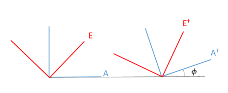
Figure 3: The virtual rotation of the detector tensors induced by the linear combination (30) of the two data channels $(A,E)$.

III.3 virtual rotation

In Sec.III A, we explained the noise independent data channels $(A,E)$ available from a single triangular detector. In fact, these two channels have an interesting property that becomes useful at correlating multiple triangular detectors (discussed in the next subsection).

To begin with, we consider the new data channels $(A^{\dagger},E^{\dagger})$ given as the linear combinations of the original ones $(A,E)$ Seto:2004ji ; Seto:2020zxw ; 1821247

$$\left(\begin{array}[]{c}{s_{A^{\dagger}}}\\ s_{E^{\dagger}}\end{array}\right)=\left(\begin{array}[]{cc}\cos 2\phi&\sin 2\phi\\ -\sin 2\phi&\cos 2\phi\end{array}\right)\left(\begin{array}[]{c}s_{A}\\ s_{E}\end{array}\right).$$ (29)

Correspondingly, the detector tensors $(\mbox{\boldmath${D}$}_{A^{\dagger}},\mbox{\boldmath${D}$}_{E^{\dagger}})$ of the new channels are given by

$$\left(\begin{array}[]{c}\mbox{\boldmath${D}$}_{A^{\dagger}}\\ \mbox{\boldmath${D}$}_{E^{\dagger}}\end{array}\right)=\left(\begin{array}[]{cc}\cos 2\phi&\sin 2\phi\\ -\sin 2\phi&\cos 2\phi\end{array}\right)\left(\begin{array}[]{c}\mbox{\boldmath${D}$}_{A}\\ \mbox{\boldmath${D}$}_{E}\end{array}\right).$$ (30)

This might look a merely formal transformation. But, after simple tensorial calculations, we can confirm that $(\mbox{\boldmath${D}$}_{A^{\dagger}},\mbox{\boldmath${D}$}_{E^{\dagger}})$ are identical to the tensors obtained by rotating the original detector tensors $(\mbox{\boldmath${D}$}_{A},\mbox{\boldmath${D}$}_{E})$ with the angle $\phi$ (see Fig.3). The factor 2 is due to the spin-2 nature of the detector tensors. Therefore, by taking the linear combinations (29), we can virtually rotate the two L-shaped detectors.

Using the relations (22) and (23), it is also straightforward to show the noise properties of the new channels $(A^{\dagger},E^{\dagger})$ as

$$\left\langle n_{A^{\dagger}}(f)n_{A^{\dagger}}(f^{\prime}{})^{*}\right\rangle=\left\langle n_{E^{\dagger}}(f)n_{E^{\dagger}}(f^{\prime}{})^{*}\right\rangle=N_{\alpha}(f)\delta(f-f^{\prime}{})$$ (31)

and

$$\left\langle n_{A^{\dagger}}(f)n_{E^{\dagger}}(f^{\prime}{})^{*}\right\rangle=0.$$ (32)

In fact, the three data channel $A,E$ and $T$ are eigenvectors of the instrumental noise matrix. The $A$ and $E$ channels have an identical eigenvalue and are orthonormal Prince:2002hp . As a result, we have freedom to readjust them with a two-dimensional rotation matrix.

III.4 symmetry of the total response function

For the triangle $\alpha$, considering the arguments in the previous subsection, the virtually rotated channels $(A^{\dagger},E^{\dagger})$ are equivalent to the original ones $(A,E)$.

Here we again consider the correlation analysis with the two triangles $\alpha$ and $\beta$. In contrast to Sec.IV B, we use the virtually rotated channels $(A^{\dagger},E^{\dagger})$ for $\alpha$ and the original ones $(A^{\prime}{},E^{\prime}{})$ for $\beta$. From the correspondence of the polarization tensors (30), the overlap reduction function for the $A^{\dagger}A^{\prime}{}$ pair is given by

$$\gamma_{A^{\dagger}A^{\prime}{}}=\gamma_{AA^{\prime}{}}\cos 2\phi+\gamma_{EA^{\prime}{}}\sin 2\phi.$$ (33)

Similarly, we have

$$\gamma_{A^{\dagger}E^{\prime}{}} = \gamma_{AE^{\prime}{}}\cos 2\phi+\gamma_{EE^{\prime}{}}\sin 2\phi,$$ (34)

$$\gamma_{E^{\dagger}A^{\prime}{}} = -\gamma_{AA^{\prime}{}}\sin 2\phi+\gamma_{EA^{\prime}{}}\cos 2\phi,$$ (35)

$$\gamma_{E^{\dagger}E^{\prime}{}} = -\gamma_{AE^{\prime}{}}\sin 2\phi+\gamma_{EE^{\prime}{}}\cos 2\phi.$$ (36)

Then we obtain

$$\gamma_{A^{\dagger}A^{\prime}{}}^{2}+\gamma_{A^{\dagger}E^{\prime}{}}^{2}+\gamma_{E^{\dagger}A^{\prime}{}}^{2}+\gamma_{E^{\dagger}E^{\prime}{}}^{2}$$

$$= \gamma_{AA^{\prime}{}}^{2}+\gamma_{AE^{\prime}{}}^{2}+\gamma_{EA^{\prime}{}}^{2}+\gamma_{EE^{\prime}{}}^{2}.$$

$$= Y_{\alpha\beta}$$ (38)

This geometrically means that, with respect to the the total response function $Y_{\alpha\beta}$, we do not have a preferred rotation angle $\phi$ for the two L-shaped interferometers associated with $\alpha$. In fact, this rotational invariance holds not only for the function $Y_{\alpha\beta}$ but also for each tensorial factor $X_{ij}$. We can easily understand this from the quadratic dependence on the detector tensors $D_{a,ij}$ as shown in Eqs.(27) and (28). From the symmetry of the system, we can make the same arguments for the second triangle $\beta$.

III.5 expressions with three cosines

The tensorial factors $X_{ij}$ are given by the unit directional vector ${m}$ and the four detector tensors $\mbox{\boldmath${D}$}_{a,ij}$ ($a=A,E,A^{\prime}{},E^{\prime}{})$ generated from the two triangles $\alpha$ and $\beta$. We need rather complicated manipulations for evaluating the tensorial factors $X_{ij}$ with the expressions such as Eqs.(27) and (28). In this subsection, we examine how we can simplify the tensorial factors by using the rotational symmetry discussed in the previous subsection.

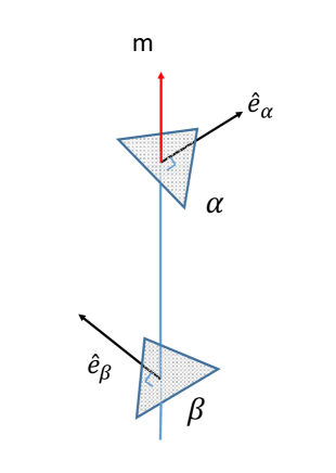
Figure 4: Configuration of the two triangles $\alpha$ and $\beta$. The unit vector ${m}$ shows the direction from $\beta$ to $\alpha$. We put $\hat{\mbox{\boldmath${e}$}}_{\alpha}$ and $\hat{\mbox{\boldmath${e}$}}_{\beta}$ as the unit normal vectors to the triangle planes. We characterize the geometry of this system using the three cosines $\rm{c_{\alpha}}\equiv\hat{\mbox{\boldmath${e}$}}_{\alpha}\cdot\mbox{\boldmath${m}$},~{}~{}\rm{c_{\beta}}\equiv\hat{\mbox{\boldmath${e}$}}_{\beta}\cdot\mbox{\boldmath${m}$}$ and $\rm{c_{\alpha\beta}}\equiv\hat{\mbox{\boldmath${e}$}}_{\alpha}\cdot\hat{\mbox{\boldmath${e}$}}_{\beta}$.

Here the key point is that the factors $X_{ij}$ do not depend on the rotations of the tensors $(\mbox{\boldmath${D}$}_{A},\mbox{\boldmath${D}$}_{E})$ and $(\mbox{\boldmath${D}$}_{A^{\prime}{}},\mbox{\boldmath${D}$}_{E^{\prime}{}})$ respectively on their detector planes. Then, for the factors $X_{ij}$, the information of the detector tensors should be completely specified by the unit vectors $\hat{\mbox{\boldmath${e}$}}_{\alpha}$ and $\hat{\mbox{\boldmath${e}$}}_{\beta}$ respectively normal to the two detector planes (see Fig.4). As a result, the factors $X_{ij}$ should be written by the three vectors $\hat{\mbox{\boldmath${e}$}}_{\alpha},\hat{\mbox{\boldmath${e}$}}_{\beta}$ and ${m}$ with totally six degrees of freedom. But our observational target is an isotropic background, and the factors $X_{ij}$ should not be changed by the overall three-dimensional rotation of the network (characterized by the three Euler angles).

For the remaining three degrees of freedom, we select the three cosines given by the inner products of the three unit vectors

$$\rm{c_{\alpha}}\equiv\hat{\mbox{\boldmath${e}$}}_{\alpha}\cdot\mbox{\boldmath${m}$},~{}~{}\rm{c_{\beta}}\equiv\hat{\mbox{\boldmath${e}$}}_{\beta}\cdot\mbox{\boldmath${m}$},~{}~{}\rm{c_{\alpha\beta}}\equiv\hat{\mbox{\boldmath${e}$}}_{\alpha}\cdot\hat{\mbox{\boldmath${e}$}}_{\beta}.$$ (39)

In fact, we can rewrite the tensorial factors $X_{ij}$ in terms of the three cosines as follows

$$X_{00} = \frac{1}{16}\left(1+6\rm{c_{\alpha\beta}}^{2}+\rm{c_{\alpha\beta}}^{4}\right)$$ (40)

$$X_{11} = \frac{1}{16}\left(1+\rm{c_{\alpha\beta}}^{2}\right)(1-\rm{c_{\alpha}}^{2})(1-\rm{c_{\beta}}^{2})$$ (41)

$$X_{22} = \frac{1}{16}(1-\rm{c_{\alpha}}^{2})^{2}(1-\rm{c_{\beta}}^{2})^{2}$$ (42)

$$X_{01} = \frac{1}{16}[1-\rm{c_{\alpha}}^{2}-\rm{c_{\beta}}^{2}-\rm{c_{\alpha\beta}}\rm{c_{\alpha}}\rm{c_{\beta}}+\rm{c_{\alpha\beta}}^{3}\rm{c_{\alpha}}\rm{c_{\beta}}$$ (43)

$$-\rm{c_{\alpha\beta}}^{2}(\rm{c_{\alpha}}^{2}+\rm{c_{\beta}}^{2}-3)]$$

$$X_{02} = \frac{1}{16}[\rm{c_{\alpha\beta}}^{2}(1+\rm{c_{\alpha}}^{2})(1+\rm{c_{\beta}}^{2})-4\rm{c_{\alpha\beta}}\rm{c_{\alpha}}\rm{c_{\beta}}(\rm{c_{\alpha}}^{2}+\rm{c_{\beta}}^{2})$$ (44)

$$+(2\rm{c_{\alpha}}^{2}+\rm{c_{\beta}}^{2}-1)(2\rm{c_{\beta}}^{2}+\rm{c_{\alpha}}^{2}-1)]$$

$$X_{12} = \frac{1}{16}(1-\rm{c_{\alpha}}^{2})(1-\rm{c_{\beta}}^{2})$$ (45)

$$\times(1-\rm{c_{\alpha}}^{2}-\rm{c_{\beta}}^{2}+\rm{c_{\alpha}}\rm{c_{\beta}}\rm{c_{\alpha\beta}}).$$

We can easily check these expressions using a software such as $Mathematica$. Therefore, the total response function $Y_{\alpha\beta}$ is formally expressed as

$$Y_{\alpha\beta}=~{}\sum_{i=0}^{2}\sum_{j=0}^{2}b_{i}(y)b_{j}(y)X_{ij}(\rm{c_{\alpha}},\rm{c_{\beta}},\rm{c_{\alpha\beta}})$$ (46)

with the argument $y=2\pi fd/c$ for the wave factors $b_{i}(y)$.

III.6 some remarks

Here we make some remarks about the tensorial factors. In general, the three cosines in Eqs.(39) do not uniquely determine the three-dimensional homothetic structure of the network. As in the case of molecular structures of optically active materials, we cannot distinguish the configuration shown in Fig.4 from its mirrored counterpart (with some exceptions including those in Sec. IV). But the two (original and mirrored) networks have an identical sensitivity at least for the parity even quantities as studied in this paper.

As shown in Eqs.(40)-(45), the tensorial factors are given as polynomials of three cosines. There are three simple relations for the indexes $n_{\alpha},n_{\beta}$ and $n_{\alpha\beta}$ of the involved terms $\rm{c_{\alpha}}^{\it n_{\alpha}}\rm{c_{\beta}}^{\it n_{\beta}}\rm{c_{\alpha\beta}}^{\it n_{\alpha\beta}}$. First, if we interchange the two labels $\alpha$ and $\beta$, the unit vector flips $\mbox{\boldmath${m}$}\to-\mbox{\boldmath${m}$}$. Correspondingly, $\rm{c_{\alpha}}$ and $\rm{c_{\beta}}$ change their signs, and the summation $n_{\alpha}+n_{\beta}$ must be an even number to keep the factors $X_{ij}$ unchanged. In addition, the factors should be invariant for the replacement $\hat{\mbox{\boldmath${e}$}}_{\alpha}\to-\hat{\mbox{\boldmath${e}$}}_{\alpha}$, and $n_{\alpha}+n_{\alpha\beta}$ becomes an even number. Similarly, $n_{\beta}+n_{\alpha\beta}$ must be even for the flip $\hat{\mbox{\boldmath${e}$}}_{\beta}\to-\hat{\mbox{\boldmath${e}$}}_{\beta}$. We can observe these relations for the power indexes in Eqs.(40)-(45).

In fact, without loss of generality, we only need to consider the ranges $\rm{c_{\alpha}}\geq 0$ and $\rm{c_{\beta}}\geq 0$. But, for simplicity, we do not introduce these limitations.

IV special cases

Our expression (46) (together with Eqs.(17)-(19) and (40)-(45)) is given for two triangular detectors with general network configuration as shown in Fig.4. We can simplify it, when a network has a special geometrical symmetry. In this section, we briefly discuss three representative examples. They have inclusion relations.

IV.1 linearly dependent

If the three vectors $\hat{\mbox{\boldmath${e}$}}_{\alpha},\hat{\mbox{\boldmath${e}$}}_{\beta}$ and ${m}$ are linearly dependent, we can express the three cosines with two parameters as

$$\rm{c_{\alpha}}=\sin\rho,\rm{c_{\beta}}=\sin\sigma,\rm{c_{\alpha\beta}}=\cos(\rho+\sigma).$$ (47)

Then we can show

$$X_{11}=X_{02}.$$ (48)

If the two triangles are tangent to a sphere (as for the LISA-Taiji network Seto:2020zxw ; 1821247 ), the three vectors are linearly dependent. In this case, we can put

$$\rm{c_{\alpha}}=\sin(\rho/2),\rm{c_{\beta}}=\sin(\rho/2),\rm{c_{\alpha\beta}}=\cos\rho.$$ (49)

Here $\rho$ is the opening angle between the two triangles measured from the center of the sphere. After some calculations, we can recover the results presented in the literature Seto:2020zxw ; 1821247

$$Y_{\alpha\beta}=2\Theta_{1}^{2}+2\Theta_{2}^{2}$$ (50)

with

$$\Theta_{1} = \cos^{4}\left(\frac{\rho}{2}\right)\left(j_{0}+\frac{5}{7}j_{2}+\frac{3}{112}j_{4}\right)$$ (51)

$$\Theta_{2} = \left(-\frac{3}{8}j_{0}+\frac{45}{56}j_{2}-\frac{169}{896}j_{4}\right)$$ (52)

$$+\left(\frac{1}{2}j_{0}-\frac{5}{7}j_{2}-\frac{27}{224}j_{4}\right)\cos\rho$$

$$+\left(-\frac{1}{8}j_{0}-\frac{5}{56}j_{2}-\frac{3}{896}j_{4}\right)\cos 2\rho.$$

These expressions might be used for studying correlation analysis with two ET-like triangular detectors on the Earth.

IV.2 normal direction

As a subset of linearly dependent configurations, we consider the case when one of the triangle (say $\alpha$) is normal to the the direction vector ${m}$ ($\rm{c_{\alpha}}=\pm 1$). From the relations $D_{A,ij}m_{i}=D_{E,ij}m_{i}=0$, only the factor $X_{00}=0$ is non-vanishing, and we obtain

$$Y_{\alpha\beta}=b_{0}(y)^{2}X_{00}(\rm{c_{\alpha\beta}}).$$ (53)

IV.3 collocated triangles

If the barycenter of the two triangles are at the same place ($d=0$), we have $y=0$. This can be regarded as a subset of the previous subsection. Using the relation

$$j_{n}(0)=\delta_{n0},$$ (54)

we obtain

$$Y_{\alpha\beta}=4X_{00}(\rm{c_{\alpha\beta}}).$$ (55)

Later, we will apply this expression for correlation analysis with two TianQin units. Eq.(55) is also the result at the low frequency limit $y\ll 1$ for general network configurations.

V Tensorial factors for LISA, TianQin and Taiji

In this section, we first present basic geometrical information of LISA, Taiji and TianQin. Then, we evaluate the tensorial factors $X_{ij}$ for their representative pairs.

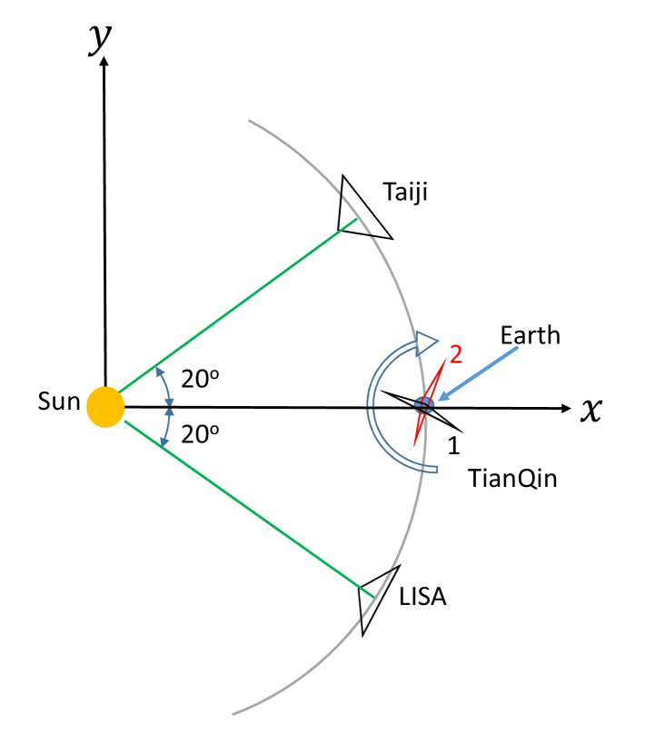
Figure 5: Schematic picture for the configurations of LISA, Taiji and TianQin. We use the frame co-rotating with the Earth. The $x$- and $y$-axes are on the ecliptic plane. The two triangles for LISA and Taiji are effectively fixed in this frame. TianQin is a geocentric project and uses up to 2 triangle units; TianQin1 and TianQin2. Their normal vectors rotate in 1 year period.

V.1 basic geometrical parameters

Fig.5 shows the planned positions of the three projects in the coordinate system co-rotating with the Earth around the Sun. Here the $xy$-plane is the ecliptic plane. As for the orientation of each triangles, considering the argument in section III E, we just need to specify their normal vectors.

LISA is a heliocentric detector at $20^{\circ}$ behind the Earth. In the co-rotating frame, its normal vector is given by

$$\hat{\mbox{\boldmath${e}$}}_{L}=\left(-\frac{\sqrt{3}\cos 20^{\circ}}{2},\frac{\sqrt{3}\sin 20^{\circ}}{2},\frac{1}{2}\right)$$ (56)

with the label $L$ for LISA.

The configuration of Taiji (labeled $J$) is similar to LISA but at $20^{\circ}$ ahead of the Earth. Its normal vector is given by

$$\hat{\mbox{\boldmath${e}$}}_{J}=\left(-\frac{\sqrt{3}\cos 20^{\circ}}{2},-\frac{\sqrt{3}\sin 20^{\circ}}{2},\frac{1}{2}\right).$$ (57)

For comparison, we consider a mirrored image of the Taiji triangle with respect to the ecliptic plane 1821247 . The resultant triangle (labeled $J^{\prime}{}$) can be composed by three heliocentric orbits, and its normal vector is given by

$$\hat{\mbox{\boldmath${e}$}}_{J^{\prime}{}}=\left(-\frac{\sqrt{3}\cos 20^{\circ}}{2},-\frac{\sqrt{3}\sin 20^{\circ}}{2},-\frac{1}{2}\right).$$ (58)

For the $LJ$ pair, we have a virtual sphere that simultaneously contact with the two triangles Seto:2020zxw ; 1821247 . But this is not the case for the $LJ^{\prime}{}$ pair.

TianQin is a geocentric project and is planned to use up to two triangle units; TianQin1 and 2 (respectively with the labels $Q$ and $Q^{\prime}{}$) Huang:2020rjf . The normal vector of TianQin1 is given by

$$\hat{\mbox{\boldmath${e}$}}_{Q}(t)=(-\cos\phi\cos\zeta,\sin\phi\cos\zeta,-\sin\zeta)$$ (59)

that rotates at 1 year period parameterized by

$$\phi\equiv 2\pi\left(\frac{t}{\rm 1yr}\right).$$ (60)

In a non-rotating frame, the normal vector $\hat{\mbox{\boldmath${e}$}}_{Q}$ is fixed and directed to the known binary RX J0806.3+1527 Luo:2015ght ; Huang:2020rjf . Here $\zeta=4.7^{\circ}$ is the small offset angle between the binary and the ecliptic plane.

The normal vector of TianQin2 (in the co-rotating frame) is given by

$$\hat{\mbox{\boldmath${e}$}}_{Q^{\prime}{}}(t)=[-\cos(\phi-\pi/2),\sin(\phi-\pi/2),0]$$ (61)

with the same parametrization as Eq.(60) Huang:2020rjf . We have $\hat{\mbox{\boldmath${e}$}}_{Q^{\prime}{}}(t)\cdot\hat{\mbox{\boldmath${e}$}}_{Q}(t)=0$. Even with the small misalignment angle $\zeta$, we also have $\hat{\mbox{\boldmath${e}$}}_{Q^{\prime}{}}(t+1/4)\simeq\hat{\mbox{\boldmath${e}$}}_{Q}(t)$.

In the original report of TianQin Luo:2015ght , the basic mission parameters are presented for a single triangular unit whose normal vector is identical to $\hat{\mbox{\boldmath${e}$}}_{Q}$. According to the report, the observational windows of the unit might be $2\times(3\,\rm months)$ per one year. This reflects the instrumental design to suppress the mission cost in relation to the solar radiation. If we simply follow this operation schedule, taking into account of the relative direction to the Sun, the duty cycles of TianQin1 and TianQin2 would be at most 50%, without overlapped period. In this case, the possibility of correlation analysis is excluded. Below, we optimistically assume that the two units have 100% duty cycles (thus completely overlapped, see e.g. Huang:2020rjf )

Using the geometrical parameters presented in this subsection, we next evaluate the tensorial factors $X_{ij}$ and the total response functions $Y_{\alpha\beta}(f)$ for some of the detector pairs.

V.2 LISA-Taiji network

The LISA-Taiji network has the separation $d=1{\rm AU}\times 2\sin 20^{\circ}=1.0\times 10^{8}$km with the unit directional vector

$$\mbox{\boldmath${m}$}=(0,1,0)~{}~{}$$ (62)

in the co-rotating frame. Then, using expressions (40)-(45), we have

$$X_{00} = 0.346,X_{11}=0.087,X_{22}=0.043,$$ (63)

$$X_{01} = 0.173,X_{02}=0.087,X_{12}=0.039.$$ (64)

As shown in Eq.(48), we have $X_{11}=X_{02}$ for this symmetric network. We present the total response function $Y_{LJ}$ in Fig.6. We have $Y_{LJ}(f)\ll 1$ around $f\sim 2$mHz, as pointed out in Seto:2020zxw ; 1821247 .

We also evaluate the tensorial factors for the $LJ^{\prime}{}$ pair and obtain

$${X}_{00} = 0.103,{X}_{11}=0.057,{X}_{22}=0.043,$$ (65)

$${X}_{01} = 0.072,{X}_{02}=0.043,{X}_{12}=0.041.$$ (66)

As shown in Fig.6, the asymptotic value $Y_{LJ^{\prime}{}}(f=0)$ is smaller than that of the $LJ$ pair, but we have $Y_{LJ^{\prime}{}}(f)\gg Y_{LJ}(f)$ around 2mHz.

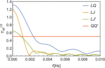
Figure 6: The total response function $Y_{\alpha\beta}(f)$ for the four pairs; LISA-TianQin ($LQ$), LISA-Taiji ($LJ$), its variation ($LJ^{\prime}{}$) and TianQin1-TianQin2 ($QQ^{\prime}{}$).

V.3 LISA-TianQin network

The LISA-TianQin1 ($LQ$) network has the distance $d=1{\rm AU}\times 2\sin 10^{\circ}=5.2\times 10^{7}$km and the unit directional vector

$$\mbox{\boldmath${m}$}=(-\cos 80^{\circ},-\sin 20^{\circ},0).~{}~{}$$ (67)

While the wave factors $b_{i}(y)$ are time independent, the tensorial factors $X_{ij}$ change with time due to the annual rotation of the normal vector $\hat{\mbox{\boldmath${e}$}}_{Q}$ as in Eq.(59). But we can easily take their time averages appropriate for the total signal-to-noise ratio;

$$\bar{X}_{ij}=\frac{1}{2\pi}\int_{0}^{2\pi}X_{ij}d\phi.$$ (68)

We numerically obtain

$$\bar{X}_{00} = 0.432,\bar{X}_{11}=0.095,\bar{X}_{22}=0.045,$$ (69)

$$\bar{X}_{01} = 0.186,\bar{X}_{02}=0.086,\bar{X}_{12}=0.045,$$ (70)

and plot the total response function $Y_{LQ}(f)$ in Fig.6 with

$${Y}_{LQ}=~{}\sum_{i=0}^{2}\sum_{j=0}^{2}b_{i}(y)b_{j}(y){\bar{X}}_{ij}.$$ (71)

Similarly we can evaluate the tensorial factors for the LISA-TianQin2 ($LQ^{\prime}{}$) network. The two networks $LQ$ and $LQ^{\prime}{}$ have slightly different tensorial factors due to the small misalignment angle $\zeta$. But, except for $X_{00}=0.432104$($LQ$) and $X_{00}=0.432617$$(LQ^{\prime}{})$, they have no difference in the significant digits used in Eqs.(69) and (70). From the geometrical symmetry, we also have $Y_{LQ}=Y_{JQ}$ and $Y_{LQ^{\prime}{}}=Y_{JQ^{\prime}{}}$.

V.4 TianQin1-2 network

From Eqs.(55) with $\rm{c_{\alpha\beta}}=\hat{\mbox{\boldmath${e}$}}_{Q}\cdot\hat{\mbox{\boldmath${e}$}}_{Q^{\prime}{}}=0$, we have

$$Y_{QQ^{\prime}{}}=\frac{1}{4}.$$ (72)

VI signal-to-noise ratio

As shown in Eq.(24), for two triangle detectors $\alpha$ and $\beta$, the total signal-to-noise ratio is given by

$$SNR_{\alpha\beta}^{2}=\left(\frac{3H_{0}^{2}}{10\pi^{2}}\right)^{2}T_{\rm obs}\left[2\int_{f_{\rm min}}^{f_{\rm max}}df\frac{\Omega_{\rm GW}(f)^{2}Y_{\alpha\beta}(f)}{f^{6}N_{\alpha}(f)N_{\beta}(f)}\right]$$ (73)

with the total response function $Y_{\alpha\beta}(f)$. In this section, we first present the noise spectra $N_{\alpha}(f)$ for the three projects and then numerically evaluate the total signal-to-noise ratios. Note that, even for the rather complicated LISA-TianQin1 pair, with our formulation based on Eq.(46), we can separately deal with the time and frequency integrals (see also Eq.(68)).

VI.1 instrumental noise spectra

The arm length of LISA is $R_{L}=2.5\times 10^{6}$km with the associated characteristic frequency $f_{L}=c/(2\pi R_{L})=0.019$Hz. The low frequency approximation is efficient in the range $f<f_{L}$. The noise spectrum of LISA’s $A$ and $E$ channels is approximately given by Cornish:2018dyw

$$N_{L}(f) = \frac{4}{3R_{L}^{2}}\left[P_{o1}+2[1+\cos(f/f_{L})^{2}]\frac{P_{a1}}{(2\pi f)^{4}}\right]$$ (74)

$$\times[1+0.6(f/f_{L})^{2}].$$

Here the acceleration noise and the optical path noise are respectively given by

$$P_{a1} = 9.0\times 10^{-30}[1+(4\times 10^{-4}/f)^{2}]$$ (75)

$$\times(1+[f/(8\times 10^{-3})]^{4}){\rm m^{2}s^{-4}Hz^{-1}}$$

$$P_{o1}=2.25\times 10^{-22}[1+(2\times 10^{-3}/f)^{4}]{\rm Hz^{-1}}.$$ (76)

In Eq.(74) we did not include the angular averages for the beam pattern functions (a factor 2/5 times smaller than Cornish:2018dyw ). The noise spectrum $N_{L}(f)$ is presented in Fig.1.

Taiji has the arm length $R_{J}=3.0\times 10^{6}$km with the characteristic frequency $f_{J}=c/(2\pi R_{J})=0.016$Hz. Using the same functional forms as Eqs.(75) and (76), its noise spectrum is given by Wang:2020vkg

$$N_{J}(f) = \frac{4}{3R_{b}^{2}}\left[0.8^{2}P_{o1}+2[1+\cos(f/f_{b})^{2}]\frac{P_{a1}}{(2\pi f)^{4}}\right]$$ (77)

$$\times[1+0.6(f/f_{b})^{2}].$$

We put $N_{J^{\prime}{}}(f)=N_{J}(f)$ for the slightly different configuration.

The triangular units of TianQin have the arm length $R_{Q}=1.7\times 10^{6}$km much smaller than LISA and Taiji. The characteristic frequency for the low frequency approximation is $f_{Q}=c/(2\pi R_{Q})=0.28$Hz. The noise spectrum for its $A$ and $E$ data channels is approximately given by Huang:2020rjf

$$N_{Q}(f) = \frac{4}{3L_{Q}^{2}}\left[P_{o2}+\frac{4P_{a2}}{(2\pi f)^{4}}\left(1+\frac{\rm 0.1mHz}{f}\right)\right]$$ (78)

$$\times[1+0.6(f/f_{Q})^{2}]$$

with $P_{a2}=1.0\times 10^{-30}{\rm m^{2}s^{-4}Hz^{-1}}$ and $P_{o2}=1.0\times 10^{-24}{\rm m^{2}Hz^{-1}}$.

VI.2 numerical results

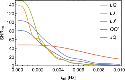
Figure 7: The signal-to-noise ratios $SNR_{\alpha\beta}$ as functions of the low frequency cut-off frequency $f_{\rm min}$. We assume a flat spectrum $\Omega_{GW}=10^{-11}$ and the integration period $T_{obs}=10$yr.

Now we numerically evaluate the total $SNR_{\alpha\beta}$ for some pairs of detectors. As a fiducial model of the background spectrum $\Omega_{GW}(f)$, we use the following flat model

$$\Omega_{GW}=10^{-11}.$$ (79)

In Eq.(73), we take the maximum frequency at $f_{\rm max}=0.1$Hz and fix the integration period at $T_{\rm obs}=10$yr. We set the minimum frequency $f_{\rm min}$ as a free parameter. In reality, the frequency $f_{\rm min}$ should be determined by the subtraction of the Galactic binary foreground, and is closely related to the integration period $T_{\rm obs}$ Cornish:2018dyw . In typical astronomical models, the expected value would be $f_{\rm min}=2\sim$5mHz for observational periods 4-10yr.

In Fig.7, our numerical results are presented as functions of $f_{\rm min}$. Using this figure, we first discuss the validity of the low frequency approximation for our calculations. As mentioned in the previous subsection, this approximation does not work above the characteristic frequency $f_{\alpha}=c/(2\pi R_{\alpha})(\geq f_{J}=16$mHz) determined by the arm length $R_{\alpha}$ of the detector $\alpha$. But as shown in Fig.7, the contributions of the signals above 8mHz are negligible, except for the $QQ^{\prime}{}$-pair. Even in the case of the $QQ^{\prime}{}$-pair, we have only $SNR_{QQ^{\prime}{}}=1.12$ for $f_{\rm min}=30$mHz$\ll f_{Q}=$280mHz, and the contribution from $f\gtrsim f_{Q}$ is negligible. Therefore, in all cases, we can safely apply the low frequency approximation for estimating $SNR_{\alpha\beta}$ presented in Fig.7. The signal-to-noise ratio is given by the frequency integral (73) of the product $Y_{\alpha\beta}(f)\cdot f^{-6}\cdot(N_{\alpha}N_{\beta})^{-1}$ and the factor $f^{-6}$ strongly suppresses the contribution of the high frequency part. Unless the input spectrum $\Omega_{GW}(f)$ is heavily blue tilted, the low frequency approximation works efficiently.

For the combination of a realistic cut-off $f_{\rm min}=2.5$mHz and a somewhat optimistic overlapped time $T_{\rm obs}=10$yr, the signal-to-noise ratios are in a relatively narrow range 50-75. For the threshold $SNR_{\alpha\beta}=10$, the detection limits are roughly given by $\Omega_{GW}\sim 2\times 10^{-12}$.

Next, we discuss the characteristic aspects of individual curves in Fig.7. The result for the $LJ$ pair was already studied in Seto:2020zxw , but we briefly mention its basic profile for comparison with other cases. In Fig.7, for the $LJ$ pair, we can observe a flat region around $f_{\rm min}\sim 2$mHz. This reflects the deep dip of the total response function $Y_{LJ}\ll 1$ at $f\sim 2$mHz (see Fig.6). For the $LJ^{\prime}{}$-pair, we can observe a similar but less prominent modulations around 3mHz, 4mHz and 6mHz, corresponding to the dips of the total response function $Y_{LJ^{\prime}{}}$. On the whole, affected by the difference around 2mHz, we have $SNR_{LJ}<SNR_{LJ^{\prime}{}}$ for $f_{\rm min}\lesssim 2.3$mHz. This inequality might be interesting for planning potential collaboration between LISA and Taiji.

As shown in Fig.7, the $QQ^{\prime}{}$-pair could be a powerful probe for the frequency regime $f\gtrsim$5mHz, compared with other combinations. This curve is for our optimistic assumption with 100% duty cycle in 10 years. Even with the total overlapped time of 2 years, the expected signal-to-nose ratio is obtained by multiplying the factor $0.2^{1/2}=0.45$ to the result $SNR_{QQ^{\prime}{}}$ given in Fig.7. We can still keep the sensitivity level $\Omega_{GW}\lesssim 10^{-11}$.

In Fig.7, except for the overall scaling, the two curves for $SNR_{LQ}$ and $SNR_{JQ}$ are quite similar. Due to the symmetry of the networks $LQ$ and $JQ$, we have $Y_{LQ}=Y_{JQ}$ and the difference between the two curves is determined by the noise spectra $N_{L}(f)$ and $N_{T}(f)$ (especially at $f\lesssim 6$mHz).

VII summary and discussion

In this paper, we discussed the detectability of an isotropic gravitational wave background by correlating multiple triangular detectors such as LISA, TianQin and Taiji. In general network configurations, we still have the rotational symmetry of the data channels (Sec.III D) and, consequently, the tensorial factors $X_{ij}$ are written by the inner products of three unit vectors ${m}$, $\hat{\mbox{\boldmath${e}$}}_{\alpha}$ and $\hat{\mbox{\boldmath${e}$}}_{\beta}$ (see Fig.4). With our expression (46), we can evaluate the total response function $Y_{\alpha\beta}$ without directly dealing with detector tensors.

We evaluated the expected signal-to-noise ratios for various pairs of detectors, including correlation between LISA ($L$) and the slightly different version ($J^{\prime}{}$) of Taiji ($J$). For a cut-off frequency $f_{\rm min}\lesssim 2.3$mHz, we have $SNR_{LJ^{\prime}{}}>SNR_{LJ}$, strongly affected by the dip $Y_{LJ}\ll 1$ around 2mHz (see Fig.6).

We also pointed out that, as shown in Fig.7, the two TianQin units can play unique role to probe a background at the relatively high frequency regime $\gtrsim$5mHz. But we need to simultaneously operate its two units. It would be interesting to consider such feasibility for pursuing the advantage of the TianQin project.

In this paper, we focused our attention on the isotropic intensity of a gravitational wave background, as the most fundamental quantity. To study the background in full detail, we should examine additional properties such as the polarization states. The separation between detectors are essential for probing some of these properties Seto:2020zxw ; 1821247 ; Nishizawa:2009jh . As demonstrated in this paper, we will be able to develop simplified formulations also for the additional properties, using the three vectors characterizing the network geometry.

We have assumed that the correlation of instrumental noises is ignorable for two triangular detectors. But the actual correlation level should be carefully examined by using real data streams. Such studies can be important for the potential follow-on missions such as DECIGO Seto:2001qf ; Kawamura:2011zz and BBO Harry:2006fi .

References

(1)
J. D. Romano and N. J. Cornish,
Living Rev. Rel. 20, no.1, 2 (2017)
doi:10.1007/s41114-017-0004-1
[arXiv:1608.06889 [gr-qc]].
(2)
C. Caprini and D. G. Figueroa,
Class. Quant. Grav. 35, no.16, 163001 (2018)
doi:10.1088/1361-6382/aac608
[arXiv:1801.04268 [astro-ph.CO]].
(3)
N. Christensen,
Phys. Rev. D 46, 5250-5266 (1992)
doi:10.1103/PhysRevD.46.5250
(4)
E. E. Flanagan,
Phys. Rev. D 48, 2389 (1993).
(5)
B. Allen and J. D. Romano,
Phys. Rev. D 59, 102001 (1999).
(6)
R. W. Hellings and G. S. Downs,
Astrophys. J. Lett. 265, L39-L42 (1983)
doi:10.1086/183954
(7)
B. P. Abbott et al. [LIGO Scientific and Virgo],
Phys. Rev. D 100, no.6, 061101 (2019)
doi:10.1103/PhysRevD.100.061101
[arXiv:1903.02886 [gr-qc]].
(8)
Z. Arzoumanian et al. [NANOGrav],
[arXiv:2009.04496 [astro-ph.HE]].
(9)
P. L. Bender et al., LISA Pre-Phase A Report, Second edition, July 1998.
(10)
P. Amaro-Seoane et al.
[arXiv:1702.00786 [astro-ph]].
(11)
T. A. Prince, M. Tinto, S. L. Larson and J. Armstrong,
Phys. Rev. D 66, 122002 (2002)
doi:10.1103/PhysRevD.66.122002
[arXiv:gr-qc/0209039 [gr-qc]].
(12)
M. Tinto, J. Armstrong and F. Estabrook,
Phys. Rev. D 63, 021101 (2001)
doi:10.1103/PhysRevD.63.021101
(13)
C. J. Hogan and P. L. Bender,
Phys. Rev. D 64, 062002 (2001)
doi:10.1103/PhysRevD.64.062002
[arXiv:astro-ph/0104266 [astro-ph]].
(14)
M. R. Adams and N. J. Cornish,
Phys. Rev. D 82, 022002 (2010)
doi:10.1103/PhysRevD.82.022002
[arXiv:1002.1291 [gr-qc]].
(15)
J. Luo et al.,
Class. Quant. Grav. 33, no.3, 035010 (2016)
doi:10.1088/0264-9381/33/3/035010
[arXiv:1512.02076 [astro-ph.IM]].
(16)
W. R. Hu and Y. L. Wu, Natl. Sci. Rev. 4, 685 (2017).
(17)
N. Seto,
[arXiv:2009.02928 [gr-qc]].
(18)
H. Omiya and N. Seto,
[arXiv:2010.00771 [gr-qc]].
(19)
N. J. Cornish,
Phys. Rev. D 65, 022004 (2002)
doi:10.1103/PhysRevD.65.022004
[arXiv:gr-qc/0106058 [gr-qc]].
(20)
W. H. Ruan, C. Liu, Z. K. Guo, Y. L. Wu and R. G. Cai,
[arXiv:1909.07104 [gr-qc]].
(21)
N. Seto,
Phys. Rev. D 69, 123005 (2004)
doi:10.1103/PhysRevD.69.123005
[arXiv:gr-qc/0403014 [gr-qc]].
(22)
S. J. Huang, Y. M. Hu, V. Korol, P. C. Li, Z. C. Liang, Y. Lu, H. T. Wang, S. Yu and J. Mei,
Phys. Rev. D 102, no.6, 063021 (2020)
doi:10.1103/PhysRevD.102.063021
[arXiv:2005.07889 [astro-ph.HE]].
(23)
T. Robson, N. J. Cornish and C. Liu,
Class. Quant. Grav. 36, no.10, 105011 (2019)
doi:10.1088/1361-6382/ab1101
[arXiv:1803.01944 [astro-ph.HE]].
(24)
G. Wang, W. T. Ni, W. B. Han, S. C. Yang and X. Y. Zhong,
Phys. Rev. D 102, no.2, 024089 (2020)
doi:10.1103/PhysRevD.102.024089
[arXiv:2002.12628 [gr-qc]].
(25)
A. Nishizawa, A. Taruya and S. Kawamura,
Phys. Rev. D 81, 104043 (2010)
doi:10.1103/PhysRevD.81.104043
[arXiv:0911.0525 [gr-qc]].
(26)
N. Seto, S. Kawamura and T. Nakamura,
Phys. Rev. Lett. 87, 221103 (2001)
doi:10.1103/PhysRevLett.87.221103
[arXiv:astro-ph/0108011 [astro-ph]].
(27)
S. Kawamura, et al.
Class. Quant. Grav. 28, 094011 (2011)
doi:10.1088/0264-9381/28/9/094011
(28)
G. M. Harry, P. Fritschel, D. A. Shaddock, W. Folkner and E. S. Phinney,
Class. Quant. Grav. 23, 4887-4894 (2006)
[erratum: Class. Quant. Grav. 23, 7361 (2006)]
doi:10.1088/0264-9381/23/15/008