LAMOST Observations in 15 K2 Campaigns: I. Low resolution spectra from LAMOST DR6

Abstract

The LAMOST-K2 (LK2) project, initiated in 2015, aims to collect low-resolution spectra of targets in the K2 campaigns, similar to LAMOST-Kepler project. By the end of 2018, a total of 126 LK2 plates had been observed by LAMOST. After cross-matching the catalog of the LAMOST data release 6 (DR6) with that of the K2 approved targets, we found 160,619 usable spectra of 84,012 objects, most of which had been observed more than once. The effective temperature, surface gravity, metallicity, and radial velocity from 129,974 spectra for 70,895 objects are derived through the LAMOST Stellar Parameter Pipeline (LASP). The internal uncertainties were estimated to be 81 K, 0.15 dex, 0.09 dex and 5 kms^-1, respectively, when derived from a spectrum with a signal-to-noise ratio in the $g$ band (SNR_g) of 10. These estimates are based on results for targets with multiple visits. The external accuracies were assessed by comparing the parameters of targets in common with the APOGEE and GAIA surveys, for which we generally found linear relationships. A final calibration is provided, combining external and internal uncertainties for giants and dwarfs, separately. We foresee that these spectroscopic data will be used widely in different research fields, especially in combination with K2 photometry.

1 Introduction

The Kepler spacecraft, launched by NASA in 2009 March, had as its main scientific goal the discovery of extrasolar Earth-like planets through transit events (Koch et al., 2010). During its prime mission, Kepler collected unprecedented high-precision photometry for about 200,000 stars in a field of 115 square degrees between Cygnus and Lyrae (Borucki, 2016). In 2014, the spacecraft shifted to observe the fields along the ecliptic plane due to pointing problem caused by failure of the second reaction wheel. The data produced by K2, like the prime Kepler mission, were acquired in the short- and long-cadence modes, except that the time baseline was reduced to approximately 80 days for each campaign (Howell et al., 2014).

The K2 mission collected photometry for more than 400,000 stars during 20 campaigns (C0, C1,…, C19). Those light curves are a treasure trove for many research areas, including exoplanets (Montet et al., 2015), asteroseismology (Chen, & Li, 2018; Silvotti et al., 2019), and eclipsing binaries (Skarka et al., 2019). Nevertheless, for many applications, an in-depth exploitation of these data requires the knowledge of precise atmospheric parameters. For instance, optimal seismic models are more reliable and easier to find when the effective temperature ($T_{\rm eff}$), surface gravity ($\log g$) and metallicity ([Fe/H]) have been determined from spectroscopic measurements beforehand (Charpinet et al., 2011; Giammichele et al., 2018). Unfortunately, the Ecliptic Plane Input Catalog (EPIC; Huber et al., 2016) of the K2 sources provides atmospheric parameters derived from multi-band photometry, which do not have a high enough accuracy for the demands of asteroseismology. Therefore, to fully exploit the K2 data, many follow-up programs have been initiated. This includes spectroscopic ones, such as the Mauna Kea Spectroscopic Explorer (MSE; Bergemann et al., 2019) and Twinkle (Joshua et al., 2019) (similar to the Kepler follow-up programs APOGEE (Majewski et al., 2017; Serenelli et al., 2017; Pinsonneault et al., 2018)), the California-Kepler Survey (CKS; Petigura et al., 2017), and the K2-HERMES Survey (Wittenmyer et al., 2018), as well as photometric ones like the SkyMapper (Casagrande et al., 2019).

Based on the experience gained during previous observing campaigns, the Large Sky Area Multi-Object Fiber Spectroscopic Telescope (LAMOST, aka, Gou Shou Jing Telescope) has proved to be an ideal instrument for follow-up spectroscopic observations on targets within the Kepler field (LAMOST-Kepler project, De Cat et al., 2015; Fu et al., 2020; Zong et al., 2018). After two rounds of observations from 2012 to 2017, the LAMOST-Kepler project collected more than 220,000 spectra of 156,390 stars, providing useful parameters for exoplanet statistics (Xie et al., 2016; Dong et al., 2018; Mulders et al., 2016), precise asteroseismology (Deheuvels et al., 2014) and stellar activity (Frasca et al., 2016; Karoff et al., 2016; Yang et al., 2017).

One of the biggest obstacles in carrying out the LAMOST-Kepler project was the fact that the Kepler field is observed mainly during the summer season, when the nights available at the Xinglong Observatory are reduced due to the monsoons and the instrument maintenance. Unlike Kepler, the K2 mission has a much wider sky coverage, consisting of 20 fields identical in size to the Kepler field, uniformly distributed along the ecliptic. This has given more opportunities to observe the K2 fields with LAMOST, excluding only those with a declination lower than $-10$ degrees that are not observable. As a consequence, this has enlarged the research areas of interest from asteroseismology, stellar activity and exoplanet discovery to gravitational lensing, AGN variability, and supernovae (Howell et al., 2014). The LAMOST-K2 (LK2) project, initiated in 2015, aims to collect spectra for as many EPIC stars as possible, with the final goal of producing a very large, homogeneous catalog of atmospheric parameters for stars of various types and in different evolutionary stages, from the pre-main sequence phase to evolved objects like white dwarfs. Moreover, during its regular survey phase, LAMOST had already collected spectra for targets within several K2 campaigns before the LK2-project began. This is very valuable for the study of, for example, pulsating stars and binaries.

In this paper we summarize the main results gained from the analysis of spectra of K2 targets from the LK2project and the sixth LAMOST data release (DR6). The paper is organized as follows. In Sect. 2, we present the observations and the step we have made toward the completion of the LK2 program. Section 3 describes the library of spectra obtained within the LK2 project and during the regular LAMOST survey in the K2 fields. In Sect. 4, we present the atmospheric parameters for the LK2 stars, and discuss their uncertainties and systematics. We propose external and internal calibrations to homogenize these data with those of other spectroscopic surveys. In Sect. 5, we discuss interesting objects identified on the basis of their stellar parameters. We give a final summary in Section 6.

2 Observations

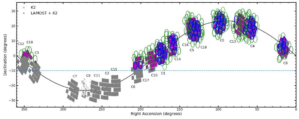
Figure 1: Sky distribution of K2 targets and LAMOST DR6 cross-matched sources in the 20 campaigns of the K2 mission. The gray symbols denote the stars with K2 photometry and the magenta dots refer to the K2 targets observed with LAMOST. The area coverage of the LK2 project and the LAMOST general survey in the K2 fields is indicated by blue and green circles, respectively. The cyan dashed line at $-10\arcdeg$ indicates the declination limit for LAMOST observations. The black solid line indicates the ecliptic plane.

LAMOST, equipped with 4000 fibers on its focal plane, is capable to simultaneously collect spectra for about 3600 targets, with a few hundreds of fibers pointing to the sky. In order to improve the efficiency of these observations, each footprint is advised to contain targets covering a certain range of magnitude. This leads to four types of LAMOST plates, namely, very bright (V), bright (B), medium-brightness (M) and faint (F) plates, respectively, according to the target brightness range (see details in Luo et al., 2012, 2015). The LK2 plates are typically V- and B-plates because K2 photometry has been collected for stars brighter than 16th magnitude. However, because the fields along the ecliptic plane, as observed for the LK2 project, are not crowded, fainter objects needed to be added to fill the fibers. Similar to the LK-project, each of the 20 K2 campaigns is divided into 14 circular fields where the central position is determined by a bright central star ($V<8$). We note that the K2 fields include a few unobserved regions corresponding to failed CCD modules on board of Kepler. No LAMOST plate was assigned in these positions. The plates within the LK2-project have a nomenclature of ’KP’+’RA’+’DEC’+’Plate type’ where ’KP’ denotes the plates belong to the projects related to follow-up observation of Kepler/K2 targets. There has been a revision of nomenclature after 2017 October, i.e. ’KP’ has been replaced by ’KII’ for the LK2-project, in order to distinguish them from those of the LK project.

The first LK2 plate was exposed in 2015 December, and a total of 126 plates has been collected until 2018 January. We acquired 1, 84, 31, and 10 plates during 1, 50, 20, and 9 nights in 2015, 2016, 2017, and 2018, respectively. We have given a higher priority to bright plates, i.e. V- and B-plates with exposures of 3$\times$600 s and 3$\times$1500 s, respectively. Additionally, there are 6 M-plates observed with an exposure time of 3$\times$1800 s each. The total shutter open time is of the order of 100 hours for all the LK2 plates, without taking overhead into account.

LAMOST performs a general regular survey of as many as possible targets across the entire northern hemisphere with declination higher than $-10$ degrees (see, e.g., Luo et al., 2012). Therefore, it is likely that several plates show overlap with some of the K2 campaigns, especially for C0 and C13 where the density of the stellar sources in the regular survey is high. We have also collected the spectra of these common targets in our library, based on the criteria in section 3.1. However, most of them have only a few targets in common. As a consequence, 401 of these 652 plates have a number less than 100 targets with K2 photometry.

Figure 1 shows the sky coverage of all stars observed by LAMOST until DR6 stamped over the K2 photometric targets. We clearly see that the LK2 plates were observed over the campaigns with right ascension lower than 210 degrees, namely C0, C1, C4, C5, C6, C8, C10, C13, C14, C16, C17, and C18. We note that all these LK2 stamped campaigns have stars in common with the LAMOST regular survey and K2 photometry. Another three campaigns, C3, C12 and C19, are also found with common stars.

3 Spectra library

The spectral library of the present paper contains spectra of K2 sources coming from both the LK2-project and other sub-projects of the regular LAMOST survey. All these spectra can be downloaded from the LAMOST DR6 website, which contains about nine million low-resolution spectra. The calibrated spectra were produced through the 2.7.5 version of the LAMOST 2D and 1D pipelines (see Luo et al., 2015, for details).

3.1 Cross-identification

Unlike the Kepler observations that were mainly focused on asteroseismology and exoplanets (Dressing, & Charbonneau, 2013), K2 was approved to cover a wider range of astrophysical topics, including gravitational lensing (Gould, & Horne, 2013), asteroids and comets (Szabó et al., 2017), and AGNs (Edelson et al., 2013). However, we selected only stellar sources observed by the K2 mission as targets for our LAMOST low-resolution spectroscopic observations. There are 15 out of 20 K2 campaigns with a declination higher than $-10$ degree that could be observed with LAMOST (see Figure 1). They include 306 838 out of 406 270 objects collected with K2 photometry.

The cross-match of K2 and LAMOST DR6 catalogs was made with TOPCAT (Taylor, 2005), based on a criterion of distance separation less than 3.7 arcsecs, which is a bit larger than the 3.0 arcsecs of the LAMOST-Kepler project (Zong et al., 2018). This value for the search radius was adopted because the diameter of the fiber is 3.3 arcsecs and the pointing precision is 0.4 arcsecs. We note that the position of the fibers was offset for stars brighter than $V=11^{\rm m}$ to prevent saturation during exposure, but this was taken into account. Besides, we only selected spectra with signal-to-noise ratio in the SDSS $g$ band S/N_g$\geq 6$, which are mentioned as “qualified spectra” in the present paper.

The cross-match produced a final catalog that includes 160 629 low-resolution qualified spectra of 84 012 K2 objects. This amounts to 27.38% of all the observable K2 stars, or 20.68% of all the stars with K2 observations. Table 1 reports information on the observed plates, the number of sources cross-matched with the K2 catalog, and the number of sources with derived parameters. It also includes the number of sources with multiple visits. In total, more than 30,000 sources were observed more than once. The sky position of these objects is depicted in Fig. 1, which shows that almost all the K2 fields with DEC $>-10\arcdeg$ were observed with LAMOST. We note that C3, C12 and C19 can only be observed in summer time, i.e. during the monsoon season. In that period, the observing time for LAMOST is heavily reduced and the telescope is often closed for maintenance. This explains why we have very few data in these fields, as apparent from Fig. 1.

Figure 2 contains all the LK2 targets from LAMOST DR6 cross-matched with the K2 catalog. Figure 2(b) shows the distribution of the angular separation between the coordinates of the LAMOST DR6 and K2 catalogs as a function of the Kp magnitude. The higher the angular separation, the more doubtful is the cross-identification. This distribution is projected to one dimension of angular separation (Figure 2(c)) and Kp (Figure 2(a)), respectively. We find that most of the cross-matched objects ($\sim 94.36\%$) display an angular separation in the range of 0–1 arcsecs. Nevertheless, there is quite a high fraction of bright objects, with brightness in the range of 9^m–11^m, whose input coordinates have larger shifts in RA and DEC. Those targets, flagged with “offset” from DR6 catalog, should be treated with caution. Some of these have been purposely shifted to prevent saturation. If they were removed, the proportion of “large” angular separation will be reduced to a fraction of $\sim 3.6\%$. In general, our cross-identified catalog contains objects with brightness mainly in the range of 10^m–18^m, with the majority found around 12^m-16^m. This is different from the LK-project where there is a sharp decrease in the number of targets with brightness fainter than 14th magnitude (Zong et al., 2018). In the the LK2 project, the collected plates include not only V- but also some B- and M-plates. It changes the faint tail of the distribution of the magnitudes of the observed targets when compared to the LAMOST-Kepler project.

Table 1: General information of the common stars between K2 and LAMOST DR6 catalogs from 2011 to 2018. The bottom lines give the summary of the observations of the LK2-project where we give the number of targets that have been observed one (1$\times$), two (2$\times$), three (3$\times$), four (4$\times$), and at least five (+5$\times$) times.

Year	LK2 Plate	Survey Plate	Spectra	Parameter
2011	-	15	481	312
2012	-	91	15735	11874
2013	-	123	19648	16616
2014	-	130	21635	18849
2015	1	93	18003	15673
2016	84	80	47515	38758
2017	31	70	23129	17037
2018	10	50	14473	10855
Total	126	652	160619	129974
Visits			Sources	Parameter
1$\times$			48280	41634
2$\times$			20877	17445
3$\times$			8392	6827
4$\times$			3404	2753
+5$\times$			3059	2236

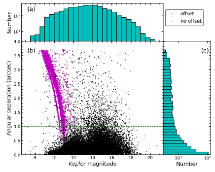
Figure 2: Angular separation between K2 and LAMOST cross-matched sources versus their Kepler magnitude (panel b) and the projected histograms (a and c). The magenta dots denote the bright sources for which the position of the LAMOST fiber was purposely offset, otherwise they are displayed as black dots. The green dashed line marks an angular separation of 1.0 arcsec.

Table 3.1 lists the catalog of the LAMOST low-resolution spectra collected for objects with K2 photometry. In the present paper we print only the first 3 lines as an example. The full table can be downloaded at LAMOST DR6 value added catalogs website, which contains the following columns:
(1) Obsid: a unique identification (ID) of the calibrated spectrum;
(2) EPIC: the cross-identified ID from the EPIC catalog where a coordinate separation of 3.7 arcsec is used as the limit (the nearest star is chosen if more than one star is identified);
(3) RA (2000): the input right ascension (epoch J2000.0) to which the fiber was pointed (in hh:mm:ss.ss);
(4) Dec. (2000): the input declination (epoch J2000.0) to which the fiber was pointed (in dd:mm:ss.ss);
(5) S/N_g: the signal-to-noise ratio (S/N) of the spectrum in SDSS g band, which is an indicator for the quality of the spectrum;
(6) Kp: the Kepler magnitude from Kepler Data Search website.
(7) SpT: the spectral type of the target, calculated by the LAMOST 1D pipeline;
(8) UTC: the Coordinated Universal Time at mid-exposure (in yyyymmddThh:mm:ss);
(9) C: the number of the K2 campaign to which the object belongs;
(10) $\Delta$d: angular separation between the equatorial coordinates of the LAMOST fiber and cross-identified source in the EPIC catalog (in arcsec);
(11) Filename: the name of the corresponding LAMOST 1D fits file.

Table 2: The spectral database of LK2 sample obtained by cross-identification of LAMOST DR6 and K2 catalogs.

Obid	EPIC	RA	Dec	S/Ng	Kp	SpT	UTC	C	$\Delta$d	Filename
		(hh:mm:ss.ss)	(dd:mm:ss.ss)		(mag)		(yyyymmddThh:mm:ss)		(arcsec)
801037	211203556	03:59:23.34	26:32:04.97	1.77	15.40	M1	20111027T18:13:00	4	0.00	spec55862B6210_sp01037.fits
801230	211189643	03:58:28.36	26:12:55.61	2.02	16.14	M0	20111027T18:13:00	4	0.00	spec55862B6210_sp01230.fits
901054	202081906	06:28:37.96	26:23:26.87	3.12	15.70	G8	20111027T20:17:00	0	0.00	spec55862B6212_sp01054.fits
…

Note. — The table has a total of 160 619 entries which can be obtained through the link abcdefgh until we are ready to submit the paper.

3.2 Spectra quality distribution

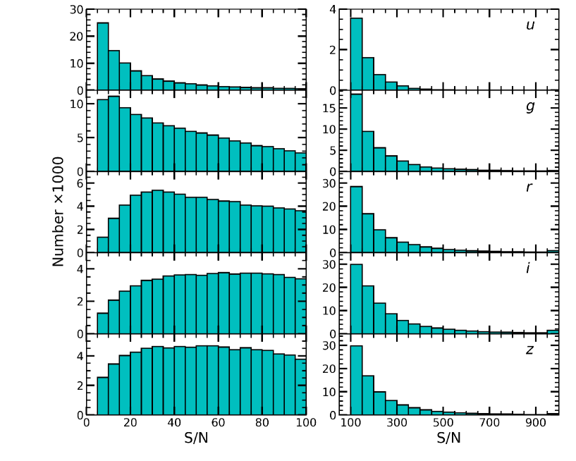
Figure 3: Distributions of the S/N in the SDSS u, g, r, i, and z bands (from top to bottom) for the spectra of LAMOST-K2 common stars. The left and right panels show the S/N ranges 6–100 and 100–1000, with bin sizes 5 and 50, respectively.

A sensitive indicator of the quality of these spectra is their S/N, typically in the SDSS $g$ band (S/N_g). Figure 3 presents the distribution of the S/N of these spectra in the SDSS $u$, $g$, $r$, $i$, and $z$ bands. The left panel shows S/N distributions in the range 6–100 with a bin size of 5, while a ten times wider range (S/N = 100–1000) is shown in the right panel with a bin size of 100. Similar to what we did in the LK-project, a spectrum is investigated by the LASP analysis pipeline for the determination of atmospheric parameters if its S/N_g is larger than 6 if it was obtained in a dark night, or larger than 15 for observations from other nights (see, e.g., Luo et al., 2015; Zong et al., 2018). The entire catalog contains 149 996, 138 880, and 86 949 spectra with S/N_g $\geq 10$, S/N_g $\geq 15$ and S/N_g $\geq 50$ corresponding to a fraction of 93.39%, 86.47% and 54.13%, respectively. This shows that LAMOST has produced a very high percentage of spectra with a good quality for the objects in K2 campaigns.

4 stellar parameters

The standard LASP pipeline was applied to the spectra of our library to derive the atmospheric parameters and radial velocities if their S/N_g was higher than the threshold values, essentially depending on spectral type. LASP incorporates two modes, the Correlation Function Interpolation (CFI, Du et al., 2012) method and the Université de Lyon Spectroscopic analysis Software (ULyss, Koleva et al., 2009; Wu et al., 2011) to determine stellar parameters. In practice, the spectral type from the LAMOST 1D pipeline is used for the first evaluation of the input spectrum. If the star is too hot or too cold (spectral type before late-A and after K), then the atmospheric parameters are not determined by LASP. For input spectra of stars with a spectral type of late-A, F, G, or K, CFI is applied to obtain initial values of $T_{\rm eff}$, $\log g$, and [Fe/H] in the following way. First, $T_{\rm eff}$ of the input spectrum is determined by comparison with synthetic spectra calculated for a grid of values of $T_{\rm eff}$. The resulting $T_{\rm eff}$-value is fixed before searching for the optimal solution in the parameter space of $\log g$ and [Fe/H]. The values with the highest reliability given by CFI are used as initial input parameters for the application of ULySS. The final LASP parameters are those giving the smallest squared difference between the observation and the model (see details in Luo et al., 2015).

A final number of 129,974 atmospheric parameters for 70,895 stars were produced with the LASP pipeline (v.2.9.7), which corresponds to a fraction of 81 % and 84 % for spectra and objects, respectively. We now count $\sim 28$ % of the observable K2 targets with homogeneously derived parameters with the same instrument and derived from the same pipeline. This is currently the largest homogeneous catalog of spectroscopically derived parameters for those targets. To properly use these data, it is necessary to do a quality control, i.e. an evaluation of the precision and accuracy of the derived parameters. To this aim we made both ”internal” tests, essentially based on the objects with multiple observations, and ”external” checks based on the comparison with parameters from the literature coming from other large spectroscopic surveys. The atmospheric parameters of some variable stars vary significantly during the period, such as eclipsing binaries, RR Lyrae stars, and other variable stars listed by Samus’ et al. (2017) and Armstrong et al. (2016). Those stars have been flagged in Table 4 in this paper. Finally, 92,853 spectra of 53,421 non-variable targets with LAMOST stellar parameters were used for the external comparison, while the internal uncertainty is estimated from 21,118 stars observed twice or more. Our data of the LK2 sample are contained in Table 4, which reports the entire catalog of parameters derived with the LASP pipeline. It contains the following columns:
(1)–(4): Same as Table 3.1,
(5) $T_{\rm eff}$: the effective temperature (in K);
(6) $\log g$: the surface gravity (in dex);
(7) [Fe/H]: the metallicity (in dex);
(8) RV: the heliocentric radial velocity (in km s^-1);
(9) Comment: Special star candidate labels, including metal-poor stars (MPs), very metal-poor stars (VMPs), high-velocity stars (HVs; cf. Section 5 for details) and the types of variable star.
All the uncertainties are provided by the LASP pipeline.

Table 3: The LK2 stellar parameter database obtained through the LASP pipeline.

Obsid	EPIC	RA	Dec	$T_{\rm eff}$	$\log g$	[Fe/H]	RV	Comment
		(hh:mm:ss.ss)	(dd:mm:ss.ss)	(K)	(dex)	(dex)	(km s-1)
407004121	201176436	11:30:41.60	04:39:42.00	4250 $\pm$ 55	4.73 $\pm$ 0.09	0.53 $\pm$ 0.05	22 $\pm$ 4	-
558704121	201176436	11:30:41.60	04:39:42.00	4232 $\pm$ 56	4.71 $\pm$ 0.09	0.51 $\pm$ 0.05	20 $\pm$ 4	-
499814067	201238068	11:36:19.20	03:23:24.00	4170 $\pm$ 55	4.67 $\pm$ 0.09	0.33 $\pm$ 0.05	7 $\pm$ 4	-
…	…	…	…	…	…	…	…	…

Note. — The table has a total of 129 974 lines, only a part is given here, the complete table is available on the data release website.

4.1 Internal uncertainties

As mentioned above, LAMOST observed a fraction of targets two or more times (see Table 1). Those objects are useful to estimate the internal uncertainties of the atmospheric parameters and RV, if we treat the values coming from different spectra of the same star as fully independent measurements randomly distributed around the mean. An unbiased way to estimate the internal errors is based on the following equations:

$$\Delta P_{i}=\sqrt{n/(n-1)}(P_{i}-\overline{P}),$$ (1)

where $i\in[0,n]$ and $n$ represent the $i$th set of values of the parameter $P_{i}$ and the total number of measurements for the same star, respectively. $\overline{P}$ denotes the average value for a given object. Equation 1 was applied to each parameter for obtaining the unbiased internal uncertainties of $\Delta$$T_{\rm eff}$, $\Delta$$\log g$, $\Delta$[Fe/H], and $\Delta$RV.

Figure 4 shows the deviations of each parameter from the average as a function of S/N_g. As expected, the deviation clearly decreases with increasing S/N_g for all parameters up to S/N_g $\sim 100$. For larger S/N_g values, the scatter seems to attain an almost constant value for all the derived quantities. We use a reciprocal function to fit those parameters and RV, in the range of S/N_g $\in[6,200]$, as

$$|\Delta P|=a_{1}\centerdot{\rm S/N}_{g}^{-1}+b_{1},$$ (2)

with a bin size of S/N_g $=10$. The coefficients, $a_{1}$ and $b_{1}$, of the best fit for each parameter are given in Table 4. According to these fitting curves, the internal errors of $T_{\rm eff}$, $\log g$, [Fe/H], and RV are 81 K, 0.0.15 dex, 0.09 dex and 5 km s^-1 when S/N_g $=10$, respectively. For S/N_g $\geq 50$, the curves tend to nearly constant uncertainties of about 28 K, 0.05 dex, 0.03 dex and 3 km s^-1 for $T_{\rm eff}$, $\log g$, [Fe/H], and RV, respectively.

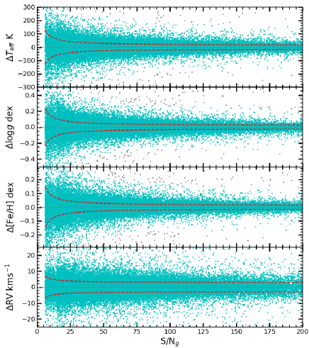
Figure 4: Scatter plots of the deviation from the mean as a function of the signal-to-noise ratio S/N_g for $T_{\rm eff}$, $\log g$, [Fe/H], and RVs (from top to bottom) for the LK2 targets with multiple visits (dots). The dashed lines represent the best fits to these data with a function of the type of Eq. 2. The gray points indicate that the outliers in the bin are beyond 6$\sigma$, and the cyan points are used for fitting.

Table 4: The coefficients of the optimal fittings for each parameters and RV.

	$T_{\rm eff}$	$\log g$	[Fe/H]	RV
$a_{1}$	668.38	1.25	0.79	23.37
$b_{1}$	14.53	0.02	0.01	2.89

4.2 External accuracy

A comparison with results of other spectroscopic surveys can help to estimate the accuracy of our parameter determination. The atmospheric parameters for K2 campaigns C0–C8 were collected from a variety of catalogs by Huber et al. (2016). However, K2 finally released 20 campaigns before it retired. We found two large surveys that contains suitable volume to compare with our data, namely the APOGEE (Apache Point Observatory Galactic Evolution Experiment: SDSS DR16 Jönsson et al., 2020) and GAIA DR2 (Gaia Collaboration et al., 2018) For our stars with multiple observations, we adopted the parameters derived from the LAMOST spectrum with the largest S/N_g. We divide non-variable targets into two samples by a sharp cut at $\log{g}_{\rm LAMOST}=3.5$ dex, where stars with $\log{g}_{\rm LAMOST}<3.5$ dex are classified as giants and the others as dwarfs. In their recent paper, Zong et al. (2020) show that the $T_{\mathrm{eff}}$ values from Gaia, which typical uncertainty is 300 K, become doubtful for stars with high extinction ($A_{G}>0.8$). Therefore, in our external comparisons we include only the RV values measured by Gaia. We found that 4,017 and 51,259 targets are overlapping with the LK2 non-variable target in APOGEE and GAIA, respectively, within 3.7 arcsec errors. We selected targets with S/N_g $>$ 15 to do a reliable comparison. Finally, we found 1,307 giant and 2,519 dwarf stars in common with APOGEE, and 20,020 stars in common with GAIA DR2.

Figure LABEL:comp shows the results of the external comparisons with other data samples: i.e. the comparison of atmospheric parameters and radial velocities between the LK2 non-variable target and APOGEE (panels a–g) and GAIA (panel h). We clearly see that $T_{\rm eff}$ agrees well between the different catalogs (panels a and b). Both the giants and dwarfs are located around the bisector for $T_{\rm eff}$. The residuals, defined here as

$$\Delta P=P_{\rm LAMOST}-P_{\rm APOGEE/GAIA},$$ (3)

are found with a bias value of $\mu=2$ and 38 K, and a standard deviation of $\sigma=83$ and 118 K for the giants and dwarfs, respectively. A linear regression, expressed as $y=a_{2}x+b_{2}$, was also applied to these plots, with the best-fit values listed in Table 5. The coefficients confirm the good agreement between the $T_{\rm eff}$ values of LK2 and APOGEE. We note there are also a few outliers whose residuals deviate more than 3$\sigma$ from the mean level. The comparison of $\log g$ values is presented in Figs. LABEL:comp(c) and (d) for giant and dwarf stars, respectively. The giants, compared to APOGEE, show consistent results in general, as further indicated by the best-fit coefficient $a_{2}=0.95$ being very close to unity. However, the $\log g$ values from LAMOST are slightly higher than those from APOGEE, with a bias of $\mu=0.12$ dex and a deviation of $\sigma=0.16$ dex. We note that the scatter becomes larger for $\log g\,\leq 2.0$ dex. The $\log g$ comparison for dwarf stars shows a slightly larger scatter. In addition, the fitting coefficient, $a_{2}=0.92$, is slightly lower than the one for the giant stars. This is evident from the slope of the residuals, which is smaller than the bisector. The results for [Fe/H] are better than those for $\log g$. We see a good agreement for [Fe/H] of giants (Fig. LABEL:comp(e)), confirmed by the best-fit coefficient $a_{2}=1.00$. The [Fe/H] comparison for dwarfs displays a linear relation with a slope of $a_{2}=1.05$. All the linear fitting coefficients are provided in Table 5. Fig. LABEL:comp(g) and LABEL:comp(h) show the RV comparison for stars in common with the APOGEE and GAIA DR2 catalogs, respectively.

The following equation provides a linear regression for RV data:

$$\left\{\begin{array}[]{l}{\rm RV}_{\rm LAMOST}=(1.00\pm 0.01)\times{\rm RV}_{\rm APOGEE}-(5\pm 1)\ {\rm km\,s}^{-1},\\ {\rm RV}_{\rm LAMOST}=(1.00\pm 0.01)\times{\rm RV}_{\rm GAIA}-(5\pm 1)\ {\rm km\,s}^{-1}.\end{array}\right.$$ (6)

It is clear that these best-fit lines are parallel to the bisectors but with a bias value of 5 km s^-1. In general, the external comparison between LK2 and APOGEE shows a good agreement for both the atmospheric parameters and RV.

Table 5: External calibration parameters.

	Giant				Dwarf
	$T_{\rm eff}$	$\log g$	[Fe/H]		$T_{\rm eff}$	$\log g$	[Fe/H]
$a_{2}$	0.97 $\pm$ 0.01	0.95 $\pm$ 0.01	1.00 $\pm$ 0.01		1.13 $\pm$ 0.01	0.92 $\pm$ 0.01	1.05 $\pm$ 0.01
$b_{2}$	147 $\pm$ 55	0.24 $\pm$ 0.02	-0.02 $\pm$ 0.01		-658 $\pm$ 28	0.35 $\pm$ 0.04	0.02 $\pm$ 0.01
$\sigma_{ex}$	83	0.16	0.07		118	0.13	0.08
$\mu_{ex}$	2	0.12	-0.01		38	0.01	0.01

4.3 Calibration of LAMOST parameters

In Sects. 4.1 and 4.2, we estimated the internal uncertainties of the atmospheric parameters and RVs derived from LK2 spectra and compared the results to two external surveys APOGEE and GAIA. On the basis of those comparisons, here we put forward calibration relations that can be used to put the LAMOST parameters on the same scale of APOGEE and GAIA data. Moreover, the linear regressions discussed in Section 4.2 provide the associated uncertainties with the propagation errors, from the following equations:

$$\left\{\begin{array}[]{l}P_{i}=(P_{i,\rm{LAMOST}}-b_{2})/a_{2},\\ \sigma_{i}=\sqrt{\sigma_{\rm{in}}^{2}+\sigma_{\rm{ex}}^{2}}.\end{array}\right.$$ (9)

where, as before, the index $i\in[1,N]$ indicates the $i$th measurement, $P_{i}$ denotes the calibrated parameters, $P_{i,\rm{\rm LAMOST}}$ represents the LAMOST parameters, and $a_{2}$ and $b_{2}$ represent the slope and the zero-point of the linear regressions whose values are reported in Table 5, $\sigma_{\rm{in}}$ is the unbiased internal error that can be calculated for each S/N_g value through Eq. (2), and $\sigma_{\rm{ex}}$ is the external deviation of the each parameter as shown in Figure LABEL:comp.

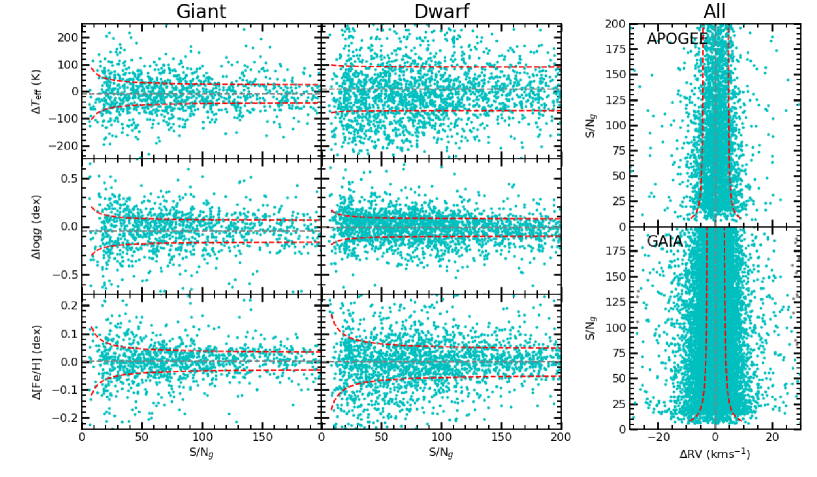
Figure 6: Distribution of the differences between LAMOST and literature parameters, $\Delta P$, after the application of both internal and external calibrations. The left panels refer to giants and dwarf, while right panels are all targets’ RVs for APOGEE and GAIA. The mean values are all close to zero and are indicated by the horizontal lines. The red dashed curves in each box represent the 1$\sigma$ levels of the best fits as a function of the S/N_g derived by means of Eq. 2. The gray points indicate that the outliers in the bin are beyond 6$\sigma$, and the cyan points are used for fitting.

The calibration is applied for each parameter independently for two groups of stars, i.e., the giants and dwarfs, distinguished on the basis of their LAMOST $\log g$ value, as explained in Section 4.2. The left panels of Figure 6 show the distributions of the differences between the calibrated LAMOST values of the atmospheric parameters ($T_{\rm eff}$, $\log g$, and [Fe/H]) and their corresponding ones in the APOGEE catalog for the giants and dwarfs while the right panels show the same for the calibrated LAMOST RV values for the stars in common with the APOGEE (top) and GAIA DR2 (bottom) catalogs. The mean values of these differences are very small for most of the derived physical quantities, which supports the good agreement between the two data sets after application of the calibrations (Eq. 9). The dispersion of the final errors are fitted with a reciprocal relation of the form of Equation 2 but with coefficients $a_{3}$ and $b_{3}$. Their best-fit values are reported in Table 6 along with $\mu$, referring to the mean values of the residuals.

Table 6: Calibration parameters.

	Giant					Dwarf
	$T_{\rm eff}$	$\log g$	[Fe/H]	RV		$T_{\rm eff}$	$\log g$	[Fe/H]	RV
$a_{3}$	519.77	1.15	0.75	35.71		64.71	0.76	1.00	51.31
$b_{3}$	31.02	0.11	0.03	4.22		80.46	0.09	0.04	2.78
$\mu$	-9	-0.05	0.00	0		9	-0.09	-0.04	0

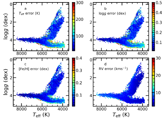
Figure 7: The Kiel ($T_{\rm eff}$ v.s. $\log g$) diagram of the LK2 samples. Note that the colors on the panels represent the calculated errors of atmospheric parameters ($T_{\rm eff}$, $\log g$, and [Fe/H]) and RV in each bin (see text for details).

Figure  7 shows the distributions of derived errors associated with atmospheric parameters across the Kiel diagram. The entire diagram are divided by a 100$\times$100 bin grid. We calculated the mean errors in each bin individually whose values are indicated by their colors. We can clearly see the errors of the stellar parameters derived with LASP are almost homogeneously distributed on the Kiel diagram, except a few values along the edge.

5 Statistical analysis of stellar parameters

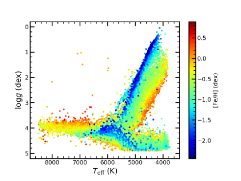
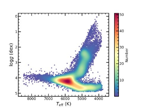
Figure 8: The Kiel diagram of the LAMOST parameters derived from the 53,421 qualified spectra of the LK2 sample. Note that the colors on the left and right panels represent [Fe/H] and density number respectively.

So far, the LAMOST-K2 project has produced 160,619 low-resolution LAMOST spectra of 84,012 stars, including 70,895 objects with derived atmospheric parameters. More than 30,000 stars were observed at multiple epochs. As shown in Figure 4, the internal uncertainties of the parameters decrease as their S/N_g increases. For objects observed more than once, we adopt the parameters derived for the spectrum with the highest S/N_g. Figure 8 shows the $\log g$ - $T_{\rm eff}$ plane (Kiel diagram) for the sources in the LK2 sample. It is apparent how most of the objects are situated on the main sequence and the giant branch, among which the main sequence is indeed the longest phase in the lifetime of a star.

As the LASP pipeline works properly for AFGK-type stars only, the $T_{\rm eff}$ values are found in the range from 3800 K to 8400 K. The values of $\log g$ are found in the range of [0, 5.0] dex. The majority of the stars have an [Fe/H] value that is close to solar, but low-metallicity stars are also present in our sample. Similar to Zong et al. (2018), the giant branch correctly displaces toward higher temperatures as [Fe/H] decreases. We also note that a slight upward trend was found in the range of low temperature on the main sequence.

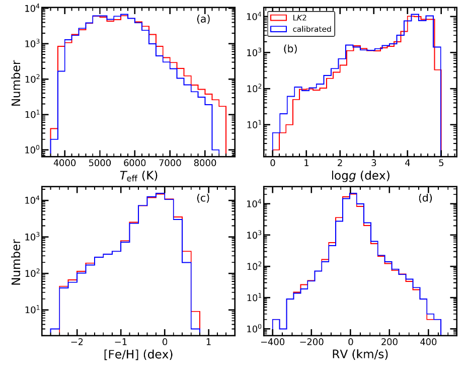
Figure 9: Distributions of stellar parameters: $T_{\rm eff}$ (a), $\log g$ (b), [Fe/H] (c), and RV (d). Original LK2 and calibrated data are represented with red and blue histograms, respectively, as indicated in the legend.

The histograms plotted in Figure 9 shows the distributions of atmospheric parameters ($T_{\rm eff}$, $\log g$, and [Fe/H]) and radial velocity (RV) before and after calibration. $T_{\rm eff}$ displays two peaks around 4800 K and 5600 K, respectively, in both data sets, which is likely the result of the projection on the $T_{\rm eff}$ axis of the main-sequence and red giant branch. The two $T_{\rm eff}$ distributions are similar to each other, but the corrected one is slightly displaced towards cool temperatures. The histogram of $\log g$ reveals a bimodal distribution with peaks around 2.4 dex and 4.2 dex, which, as before, could be the fingerprint of data clustering around the main sequence and giant branch. However, the lower peak at 2.4 dex and 0.8 dex becomes slightly clearer after applying the calibration. This might be due to the correction made by the linear relation with a small slope that smooths out the peaks.

There is hardly any difference between the distributions of [Fe/H] before and after the calibration. Most stars have a close-to solar metallicity. The two distributions of RV, before and after calibration, are very similar. They are centered around 0 km s^-1. There are few stars with $|RV|>300$ km s^-1 that can be classified as candidate high-velocity stars. In general, the distributions of the stellar parameters derived from our sample are similar to those shown by De Cat et al. (2015) and Zong et al. (2018).

6 Summary

The K2 mission has collected high-precision photometry for more than 400,000 stars with a time span of $\sim 80$ days for each source. These high-quality data pave the pathway to many different fields of astrophysics, such as asteroseismology, stellar activity and exoplanet research (Stello et al., 2015; Foreman-Mackey et al., 2015; Kennedy et al., 2018). Even though Huber et al. (2016) provide a catalog of stellar parameters for the objects in the first eight K2 campaigns, they use different methods to deduce the values of parameters and from different instruments. In the present work we report on the largest homogeneous spectroscopic dataset for the LK2 sources that is based on LAMOST spectra. Compared to the Kepler field (Zong et al., 2018), the K2 campaigns are better suited for observations with LAMOST because the even distribution of the K2 fields on the ecliptic plane fits better with the observing constraints of LAMOST, with the exception of the K2 fields with a very low declination (DEC $<\ -10\arcdeg$).

The LK2 project started in 2015 and has observed 126 plates across 15 K2 campaigns up to 2018 February. Thanks to the wide distribution of K2 fields in right ascension, there are many objects in common with other LAMOST surveys. After cross-matching the catalogs, we have collected a total of 160,619 spectra of 84,012 K2 sources from LAMOST DR6. The cross-match is based on a search radius of at maximum 3.7 arcsecs around the observed equatorial coordinates. However, the angular separation of 94.36% of the sources in the two catalogs is less than 1.0 arcsec (Figure 2). Our catalog now covers 20.68 % K2 objects spread over all the K2 campaigns observable with LAMOST. As LAMOST can only point to targets with declination higher than $-10$ degrees, the fraction of observed targets increases to 27.38 % of the all the K2 objects observable with LAMOST. The atmospheric parameters and the radial velocities provided in this paper have been derived through the LASP pipeline for 80.92% of the LK2 spectra, covering 70,895 individual K2 targets. We note, however, that the LASP works only for stars of the A, F, G, or K spectral type, and does not deliver atmospheric parameters for the O, B, and M-type stars. That is unfortunate because the latter stars are subjects of many different types of research, ranging from the search of exoplanets in the habitable zones of M-type dwarfs (Gillon et al., 2017) through the study of the internal structure of pulsating hot OB sub-dwarfs. Since those investigations rely heavily on the stars’ atmospheric parameters, it is very important to derive their values also for those stars observed in the framework of the LK2 projects which fall outside the limits of the LASP using other methods (see, e.g., Lei et al., 2019; Luo et al., 2019). That is, however, beyond the scope of this paper.

We estimated the internal uncertainties for the $T_{\rm eff}$, $\log g$, [Fe/H], and RV through the results obtained for objects with multiple visits. We found average uncertainties of 28 K, 0.05 dex, 0.03 dex and 3 km s^-1 for $T_{\rm eff}$, $\log g$, [Fe/H], and RV at S/N_g $\sim 50$, respectively. The precision improves as S/N_g increases. This result is half that of Ren et al. (2016), who found a precision of 68 K, 0.08 dex and 0.06 dex for $T_{\rm eff}$, $\log g$, and [Fe/H] at S/N_g $\sim 50$. The external accuracies of the stellar parameters of the targets of the LK2 sample are evaluated by comparison to APOGEE and GAIA DR2 catalogs, respectively. We found that, in general, our stellar parameters for giant and dwarf stars agree well with those provided by the APOGEE survey as their values are closely following a one-to-one relation.

This is possibly the result of the large errors of the dwarf values of $\log g$ and [Fe/H] in common with LK2 compared to APOGEE. These fitting slopes are likely responsible for the differences of the distributions of $T_{\rm eff}$ and $\log g$ before and after correction (see Figure 6).

In addition to the LASP pipeline, there are other codes that have been applied on the LK2 spectra, such as MKCLASS (Gray, & Corbally, 2014) and ROTFIT (Frasca et al., 2016), to derive spectral types, stellar parameters and RVs. The comparison between ROTFIT and LASP (v.2.7.5) showed that the results of both methods are in general consistent with each other (Frasca et al., 2016). As the low-resolution spectra cover almost all the visible wavelengths, they can also be used to calculate indexes of stellar activity from the equivalent width of Ca ii H and K lines (see, e.g., West et al., 2008; Karoff et al., 2016), Ca ii IRT, and H$\alpha$ (see, e.g., Frasca et al., 2016).

We recall that the LK2 program will continue in the next few years. All the spectra will be publicly available from 2021 onwards . The experiences gained from this project inspired us to initiate phase II of the LAMOST-Kepler/K2 survey, which is a new parallel program to observe time series of medium-resolution LAMOST spectra for a selection of 20 footprints distributed over the Kepler field and K2 campaigns (Zong et al., 2020). For the stars in common, the LAMOST observations with two different spectral resolutions can be analysed simultaneously for a better understanding of these sources and to study other astrophysical phenomena, such as the orbits of binaries and the short-term evolution of stellar activity. We foresee a wide usage of the spectra of the LK2 project in the near future.

References

- Armstrong et al. (2016) Armstrong, D. J., Kirk, J., Lam, K. W. F., et al. 2016, MNRAS, 456, 2260
- Bergemann et al. (2019) Bergemann, M., Huber, D., Adibekyan, V., et al. 2019, arXiv e-prints, arXiv:1903.03157
- Blanco-Cuaresma et al. (2014) Blanco-Cuaresma, S., Soubiran, C., Heiter, U., et al. 2014, A&A, 569, A111
- Borucki (2016) Borucki, W. J. 2016, Reports on Progress in Physics, 79, 036901
- Buder et al. (2018) Buder, S., Asplund, M., Duong, L., et al. 2018, MNRAS, 478, 4513
- Casagrande et al. (2019) Casagrande, L., Wolf, C., Mackey, A. D., et al. 2019, MNRAS, 482, 2770
- Charpinet et al. (2011) Charpinet, S., Van Grootel, V., Fontaine, G., et al. 2011, A&A, 530, A3
- Chen, & Li (2018) Chen, X., & Li, Y. 2018, ApJ, 866, 147
- De Cat et al. (2015) De Cat, P., Fu, J. N., Ren, A. B., et al. 2015, ApJS, 220, 19
- Deheuvels et al. (2014) Deheuvels, S., Doğan, G., Goupil, M. J., et al. 2014, A&A, 564, A27
- Dong et al. (2018) Dong, S., Xie, J.-W., Zhou, J.-L., et al. 2018, Proceedings of the National Academy of Science, 115, 266
- Dressing, & Charbonneau (2013) Dressing, C. D., & Charbonneau, D. 2013, ApJ, 767, 95
- Du et al. (2012) Du, B., Luo, A., Zhang, J., et al. 2012, Proc. SPIE, 8451, 845137
- Edelson et al. (2013) Edelson, R., Mushotzky, R., Vaughan, S., et al. 2013, ApJ, 766, 16
- Foreman-Mackey et al. (2015) Foreman-Mackey, D., Montet, B. T., Hogg, D. W., et al. 2015, ApJ, 806, 215
- Frasca et al. (2016) Frasca, A., Molenda-Żakowicz, J., De Cat, P., et al. 2016, A&A, 594, A39
- Fu et al. (2020) Fu, J. N., De Cat, P., Zong, W., et al. 2020, arXiv:2008.10776
- Gaia Collaboration et al. (2018) Gaia Collaboration, Brown, A. G. A., Vallenari, A., et al. 2018, A&A, 616, A1
- Gray, & Corbally (2014) Gray, R. O., & Corbally, C. J. 2014, AJ, 147, 80
- Giammichele et al. (2018) Giammichele, N., Charpinet, S., Fontaine, G., et al. 2018, Nature, 554, 73
- Gillon et al. (2017) Gillon, M., Triaud, A. H. M. J., Demory, B.-O., et al. 2017, Nature, 542, 456
- Gould, & Horne (2013) Gould, A., & Horne, K. 2013, ApJ, 779, L28
- Howard et al. (2012) Howard, A., Marcy, G. W., Johnson, J. A., et al. 2012, American Astronomical Society Meeting Abstracts #219 219, 405.01
- Howell et al. (2014) Howell, S. B., Sobeck, C., Haas, M., et al. 2014, PASP, 126, 398
- Huber et al. (2016) Huber, D., Bryson, S. T., Haas, M. R., et al. 2016, ApJS, 224, 2
- Joshua et al. (2019) Joshua, M., Tessenyi, M., Tinetti, G., et al. 2019, Lunar and Planetary Science Conference, 1388
- Jönsson et al. (2020) Jönsson, H., Holtzman, J. A., Prieto, C. A., et al. 2020, AJ, 160, 120
- Karoff et al. (2016) Karoff, C., Knudsen, M. F., De Cat, P., et al. 2016, Nat. Commun., 7, 11058
- Koleva et al. (2009) Koleva, M., Prugniel, P., Bouchard, A., et al. 2009, A&A, 501, 1269
- Kennedy et al. (2018) Kennedy, M. R., Clark, C. J., Voisin, G., et al. 2018, MNRAS, 477, 1120
- Koch et al. (2010) Koch, D. G., Borucki, W. J., Basri, G., et al. 2010, ApJ, 713, L79
- Kunder et al. (2017) Kunder, A., Kordopatis, G., Steinmetz, M., et al. 2017, AJ, 153, 75
- Lei et al. (2019) Lei, Z., Zhao, J., Németh, P., et al. 2019, ApJ, 881, 135
- Luo et al. (2012) Luo, A.-L., Zhang, H.-T., Zhao, Y.-H., et al. 2012, Research in Astronomy and Astrophysics, 12, 1243
- Luo et al. (2015) Luo, A.-L., Zhao, Y.-H., Zhao, G., et al. 2015, Research in Astronomy and Astrophysics, 15, 1095
- Luo et al. (2019) Luo, Y., Németh, P., Deng, L., et al. 2019, ApJ, 881, 7
- Majewski et al. (2017) Majewski, S. R., Schiavon, R. P., Frinchaboy, P. M., et al. 2017, AJ, 154, 94
- Montet et al. (2015) Montet, B. T., Morton, T. D., Foreman-Mackey, D., et al. 2015, ApJ, 809, 25
- Mulders et al. (2016) Mulders, G. D., Pascucci, I., Apai, D., Frasca, A., Molenda-Żakowicz, J. 2016, AJ, 152, 187
- Petigura et al. (2017) Petigura, E. A., Howard, A. W., Marcy, G. W., et al. 2017, AJ, 154, 107
- Pinsonneault et al. (2018) Pinsonneault, M. H., Elsworth, Y. P., Tayar, J., et al. 2018, ApJS, 239, 32
- Ren et al. (2016) Ren, A., Fu, J., De Cat, P., et al. 2016, ApJS, 225, 28
- Samus’ et al. (2017) Samus’, N. N., Kazarovets, E. V., Durlevich, O. V., et al. 2017, Astronomy Reports, 61, 80
- Serenelli et al. (2017) Serenelli, A., Johnson, J., Huber, D., et al. 2017, ApJS, 233, 23
- Silvotti et al. (2019) Silvotti, R., Uzundag, M., Baran, A. S., et al. 2019, MNRAS, 489, 4791
- Skarka et al. (2019) Skarka, M., Kabáth, P., Paunzen, E., et al. 2019, MNRAS, 487, 4230
- Stello et al. (2015) Stello, D., Huber, D., Sharma, S., et al. 2015, ApJ, 809, L3
- Szabó et al. (2017) Szabó, G. M., Pál, A., Kiss, C., et al. 2017, A&A, 599, A44
- Taylor (2005) Taylor, M. B. 2005, Astronomical Data Analysis Software and Systems XIV, 29
- West et al. (2008) West, A. A., Hawley, S. L., Bochanski, J. J., et al. 2008, AJ, 135, 785
- Wittenmyer et al. (2018) Wittenmyer, R. A., Sharma, S., Stello, D., et al. 2018, AJ, 155, 84
- Wu et al. (2011) Wu, Y., Singh, H. P., Prugniel, P., et al. 2011, A&A, 525, A71
- Xie et al. (2016) Xie, J.-W., Dong, S., Zhu, Z., et al. 2016, Proceedings of the National Academy of Science, 113, 11431
- Yang et al. (2017) Yang, H., Liu, J., Gao, Q., et al. 2017, ApJ, 849, 36
- Zong et al. (2018) Zong, W., Fu, J.-N., De Cat, P., et al. 2018, ApJS, 238, 30
- Zong et al. (2020) Zong, W., Fu, J.-N., De Cat, P., et al. 2020, arXiv:2009.06843