Minimax Q-learning Control for Linear Systems Using the Wasserstein Metric

Abstract

Stochastic optimal control usually requires an explicit dynamical model with probability distributions, which are difficult to obtain in practice. In this work, we consider the linear quadratic regulator (LQR) problem of unknown linear systems and adopt a Wasserstein penalty to address the distribution uncertainty of additive stochastic disturbances. By constructing an equivalent deterministic game of the penalized LQR problem, we propose a Q-learning method with convergence guarantees to learn an optimal minimax controller.

, [cor]Corresponding author

1 Introduction

Stochastic control is a well-studied framework for dynamical systems with known probability distributions of uncertain variables (Åström, 2012), which is usually difficult to obtain in practice. Directly using an approximated distribution is not always reliable and may even lead to system instability (Nilim & El Ghaoui, 2005). To tackle distribution errors, it is natural to use the idea of distributionally robust (DR) optimization with an appropriate distribution metric (Gao & Kleywegt, 2022; Wiesemann et al., 2014). Since the Wasserstein metric can well combine the distribution prior knowledge and sampled data (Chen & Paschalidis, 2020), it has been recently adopted to the stochastic control. Unfortunately, they require an explicit dynamical model of the control system (Yang, 2021; Kim & Yang, 2020, 2021).

Reinforcement learning (RL), as a learning-based method to approximately solve Markov decision processes (MDPs), has achieved tremendous progresses in the continuous control (Lillicrap et al., 2016). Since the RL based controller is usually trained over a simulator, it may fail to generalize to practical applications if the simulator cannot generate samples with probability distributions that correctly reflect the physical system. To tackle it, robust RL algorithms are devised to enhance the robustness of the resulting control policy (Pinto et al., 2017; Abdullah et al., 2019). For example, Abdullah et al. (2019) uses the idea of over-fitting to training environments by minimizing a long-term cost function over a Wasserstein ambiguity set. However, they only focus on the generic MDPs and may require a large number of samples, and the stability of the closed-loop system cannot be guaranteed.

This work takes advantages of both the DR optimization and RL to address the distribution uncertainty in an empirical measure of disturbance samples for unknown linear stochastic systems. Without explicitly identifying the explicit linear model, we aim to solve the minimax linear quadratic regulator (LQR) problem with a Wasserstein penalty via Q-learning. The major challenge lies in that the Q-function cannot be directly evaluated as it involves an expectation over the random disturbance, which is resolved by proposing an equivalent deterministic zero-sum game. Then, we apply Al-Tamimi et al. (2007, Section 3) to design an efficient Q-learning method with convergence guarantees to learn an optimal minimax controller.

The rest of the presentation is structured as follows. In Section 2, we describe the minimax control problem with a Wasserstein penalty and provide its closed-form solution. Section 3 designs a Q-learning algorithm to learn the minimax controller by establishing an equivalent deterministic game. Section 4 validates the convergence of the Q-learning algorithm via simulations. We draw some concluding remarks in Section 5.

2 Wasserstein minimax control

In this section, we formulate the LQR problem with a Wasserstein penalty and provide its closed-form solution.

2.1 Problem formulation

We consider a time-invariant linear stochastic system

$$x_{k+1}=Ax_{k}+Bu_{k}+Ew_{k}$$ (1)

where $(A,B,E)$ are unknown model parameters, $x_{k}\in\mathbb{R}^{n}$ is the state and $u_{k}\in\mathbb{R}^{m}$ is the control. The disturbance $\{w_{k}\}\subseteq\mathbb{R}^{d}$ is i.i.d. with an unknown probability distribution $\bf\nu$. Moreover, we have collected a finite number of disturbance samples $\{v^{j}\}_{j=1}^{N}$. Then, it is natural to use the empirical distribution, i.e., ${\nu}=\frac{1}{N}\sum_{j=1}^{N}\delta_{v^{j}}$ where the Dirac delta measure $\delta_{v^{j}}$ is concentrated at $v^{j}$.

To measure the distance between two probability distributions, we adopt the following Wasserstein metric (Gao & Kleywegt, 2022)

$$W(\mu_{1},\mu_{2})=\inf_{\kappa}\left(\int_{\mathbb{R}^{d}\times\mathbb{R}^{d}}\left\|w_{1}-w_{2}\right\|^{2}\kappa\left(\mathrm{d}w_{1},\mathrm{d}w_{2}\right)\right)^{{1}/{2}},$$

where $\|\cdot\|$ denotes the standard $l_{2}$-norm, $\kappa\in\Gamma(\mu_{1},\mu_{2})$, and $\Gamma(\mu_{1},\mu_{2})$ denotes the set of the joint distributions with marginal distributions $\mu_{1}$ and $\mu_{2}$.

To address the distributional uncertainty in ${\nu}$, we consider a zero-sum Markov game where the controller is the minimizing player and the disturbance is the maximizing player with distributions as inputs to the game. Particularly, we only focus on the deterministic policies. Let the control policy be $\{\pi_{k}\}$ that maps the history trajectory $h_{k}=\{x_{0},u_{0},\dots,x_{k}\}$ to the control input, i.e., $u_{k}=\pi_{k}(h_{k})$. Let the adversarial policy (distribution) be $\{\gamma_{k}\}$ which maps $h_{k}$ and $u_{k}$ to a distribution $\mu_{k}$, i.e., $\mu_{k}=\gamma_{k}(h_{k},u_{k})$.

Without identifying model $(A,B,E)$, this work aims to design a Q-learning algorithm via the simulator in Fig. 1 to solve a minimax control problem (Yang, 2021)

$$\min_{\{\pi_{k}\}}\max_{\{\gamma_{k}\}}\mathbb{E}^{\{\pi_{k}\},\{\gamma_{k}\}}\big{[}\sum_{k=0}^{\infty}\alpha^{k}c(x_{k},u_{k},\mu_{k})\big{]},$$ (2)

where $0<\alpha<1$ is a discount factor and $c(x_{k},u_{k},\mu_{k})=x_{k}^{\top}Qx_{k}+u_{k}^{\top}Ru_{k}-\lambda\cdot W^{2}\left(\mu_{k},{\nu}\right)$ with $Q\geq 0$ and $R>0$. The tunable hyperparameter $\lambda>0$ reflects our confidence in the empirical distribution ${\nu}$. Specifically, the larger $\lambda$, the more we trust ${\nu}$.

Figure 1: The simulator (a black-box to the control designer) produces the output of (1), which together with the input serve as samples for our learning algorithm.

2.2 Wasserstein minimax controller

In this work, we make the following assumptions.

Assumption 1.

$\Lambda=BR^{-1}B^{\top}-EE^{\top}/\lambda>0$, and $(A,\sqrt{Q})$ is observable.

Assumption 2.

$\lambda>\underline{\lambda}$ where $\underline{\lambda}=\inf\{\lambda|\lambda I-\alpha E^{\top}PE>0\},$ where $P$ is a positive semi-definite solution to

$$P=H_{xx}-\begin{bmatrix}H_{xu}&H_{xw}\end{bmatrix}\begin{bmatrix}H_{uu}&H_{uw}\\ *&H_{ww}\end{bmatrix}^{-1}\begin{bmatrix}H_{xu}^{\top}\\ H_{xw}^{\top}\end{bmatrix}$$ (3)

with $H_{xx}=Q+\alpha A^{\top}PA,H_{xu}=\alpha A^{\top}PB,H_{xw}=\alpha A^{\top}PE,H_{uu}=R+\alpha B^{\top}PB,H_{uw}=\alpha B^{\top}PE,H_{ww}=\alpha E^{\top}PE-\lambda I$.

For simplicity, define $g$ and $z$ as

$$g=G_{x}-\begin{bmatrix}H_{xu}&H_{xw}\end{bmatrix}\begin{bmatrix}H_{uu}&H_{uw}\\ *&H_{ww}\end{bmatrix}^{-1}\begin{bmatrix}G_{u}\\ G_{w}\end{bmatrix},$$ (4)

$$z=\alpha z-\lambda\|\bar{w}\|^{2}-\text{tr}\{H_{ww}^{-1}(\lambda^{2}\Sigma+\frac{1}{4}G_{w}G_{w}^{\top})\}$$

$$-\frac{1}{4}(G_{u}^{\top}-G_{w}^{\top}H_{ww}^{-1}H_{uw}^{\top})(H_{uu}-H_{uw}H_{ww}^{-1}H_{uw}^{\top})^{-1}$$

$$\times(G_{u}-H_{uw}H_{ww}^{-1}G_{w})$$

with $G_{x}=\alpha A^{\top}g,G_{u}=\alpha B^{\top}g,G_{w}=\alpha E^{\top}g+2\lambda\bar{w}$, $G_{w}^{j}=\alpha E^{\top}g+2\lambda v^{j}$.

Via a simple extension of Kim & Yang (2020), we then obtain a closed-form solution to (2).

Lemma 3.

(a) The value function $V(x)=x^{\top}Px+g^{\top}x+z$ solves the following Bellman equation

$$V(x_{k})=\min_{\{\pi_{k}\}}\max_{\{\gamma_{k}\}}\mathbb{E}^{\{\pi_{k}\},\{\gamma_{k}\}}[c(x_{k},u_{k},\mu_{k})+\alpha V(x_{k+1})].$$

(b) The minimax controller for (2) is stationary and has an affine structure, i.e., $\pi_{k}(x)=Kx+r$ where

$$K=(H_{uu}-H_{uw}H_{ww}^{-1}H_{uw}^{\top})^{-1}(H_{uw}{H_{ww}^{-1}}H_{xw}^{\top}-H_{ux}^{\top}),$$ (5)

$$r=-\frac{1}{2}(H_{uu}-H_{uw}H_{ww}^{-1}H_{uw}^{\top})^{-1}(G_{u}-H_{uw}H_{ww}^{-1}G_{w}).$$

(c) One of the least favorable adversarial policy to solve (2) is discrete and stationary. Specifically, let $w^{j}(x)=Lx+l^{j}$ with

$$L=(H_{ww}-H_{uw}^{\top}H_{uu}^{-1}H_{uw})^{-1}(H_{uw}^{\top}H_{uu}^{-1}H_{xu}^{\top}-H_{xw}^{\top}),$$ (6)

$$l^{j}=\frac{1}{2N}(H_{ww}-H_{uw}^{\top}H_{uu}^{-1}H_{uw})^{-1}(H_{uw}^{\top}H_{uu}^{-1}G_{u}-G^{j}_{w}).$$

Then, $\gamma_{k}(x,u)=\frac{1}{N}\sum_{j=1}^{N}\delta_{w^{j}}$ is a least favorable adversarial policy.

For a sufficiently large discount factor $\alpha$, it can be shown that the minimax controller in (5) can also stabilize the system; see e.g., Başar & Bernhard (2008).

Computing the minimax controller in (5) explicitly requires to know the model matrices $(A,B)$. In the sequel, we design a Q-learning algorithm to learn it via the simulator in Fig. 1.

3 The Q-learning method and convergence

In this section, we first propose a new deterministic game which has the same minimax controller as (5). Then, we develop a Q-learning algorithm with convergence guarantees to learn the minimax controller by solving the proposed deterministic game.

3.1 An equivalent deterministic game

The Q-function $Q(x_{k},u_{k},\mu_{k})$ of (2) is given by

$$Q(x_{k},u_{k},\mu_{k}) =x_{k}^{\top}Qx_{k}+u_{k}^{\top}Ru_{k}-\lambda W^{2}(\mu_{k},{\nu})$$ (7)

$$+\alpha\mathbb{E}_{w_{k}\sim\mu_{k}}[V(x_{k+1})].$$

Once Q-function is determined, an optimal controller can be easily obtained. However, it is ineffective to evaluate $Q(x_{k},u_{k},\mu_{k})$ in (7) as it involves an expectation operator. We use the Kantorovich duality (Gao & Kleywegt, 2022) and the quadratic form of $V(x)$ to resolve it. Since

$$\min_{u_{k}}\max_{\mu_{k}}Q(x_{k},u_{k},\mu_{k})=\min_{u_{k}}\{x_{k}^{\top}Qx_{k}+u_{k}^{\top}Ru_{k}$$ (8)

$$+\frac{1}{N}\sum_{j=1}^{N}\max_{w}\{\alpha V(x_{k+1})-\lambda\|w-v^{j}\|^{2}\}\}$$

$$=\min_{u_{k}}\{x_{k}^{\top}Qx_{k}+u_{k}^{\top}Ru_{k}+\max_{w_{k}}\{\alpha V(x_{k+1})$$

$$~{}~{}~{}-\lambda\|w_{k}-\bar{w}\|^{2}\}\}+z_{0}$$

where $z_{0}$ is a constant, the expectation issue in (7) can be avoided via the following deterministic zero-sum game

$$\min_{\{\tilde{\pi}_{k}\}}\max_{\{\tilde{\gamma}_{k}\}}\sum_{k=0}^{\infty}\alpha^{k}(x_{k}^{\top}Qx_{k}+u_{k}^{\top}Ru_{k}-\lambda\|w_{k}-\bar{w}\|^{2}),$$ (9)

where $\{\widetilde{\pi}_{k}\}$ is a control policy sequence in the form $u_{k}=\widetilde{\pi}_{k}(h_{k})$ and $\{\widetilde{\gamma}_{k}\}$ is a disturbance policy sequence in the form $w_{k}=\widetilde{\gamma}_{k}(h_{k},u_{k})$.

Particularly, we show in the following theorem that the minimax controller of (2) and (9) are the same.

Theorem 4.

Consider the deterministic zero-sum game in (9). We obtain the following results.

(a) The value function $V^{d}(x_{k})=\min_{u_{k}}\max_{w_{k}}(x_{k}^{\top}Qx_{k}+u_{k}^{\top}Ru_{k}-\lambda\|w_{k}-\bar{w}\|^{2}+\alpha V^{d}(x_{k+1}))$ is given by

$$\begin{array}[]{lll}V^{d}(x)&=x^{\top}Px+g^{\top}x+z-z_{0},&\\ \end{array}$$

where $P$, $g$ and $z$ are defined in (3) and (4).

(b) The Q-function $Q(x_{k},u_{k},w_{k})=x_{k}^{\top}Qx_{k}+u_{k}^{\top}Ru_{k}-\lambda\|w_{k}-\bar{w}\|^{2}+\alpha V^{d}(x_{k+1})$ is given by

$$Q(x,u,w)= \begin{bmatrix}x\\ u\\ w\end{bmatrix}^{\top}H\begin{bmatrix}x\\ u\\ w\end{bmatrix}+G^{\top}\begin{bmatrix}x\\ u\\ w\end{bmatrix}+s,$$ (10)

where $s$ is a constant scalar,

$$H =\begin{bmatrix}H_{xx}&H_{xu}&H_{xw}\\ &H_{uu}&H_{uw}\\ *&&H_{ww}\end{bmatrix},~{}\text{and}~{}G^{\top}=\begin{bmatrix}G_{x}^{\top},G_{u}^{\top},G_{w}^{\top}\end{bmatrix}.$$

(c) A minimax controller of (9) is given by (5) and a maximizing policy is given by $w(x)=Lx+l,$ where $L$ is given by (6) and

$$l=\frac{1}{2}(H_{ww}-H_{uw}^{\top}H_{uu}^{-1}H_{uw})^{-1}(H_{uw}^{\top}H_{uu}^{-1}G_{u}-G_{w}).$$

The proof is similar to that of Başar & Bernhard (2008, Theorem 3.7) and is omitted for saving space.  

The major advantage of (9) lies in that the adversarial input is no longer a sequence of distributions.

3.2 Online Q-learning algorithm to solve (2)

By (7)-(10), we now apply the results in Al-Tamimi et al. (2007, Section 3) to provide a Q-learning algorithm to learn $Q(x,u,w)$ in (10) via the simulator in Fig. 1. We first reformulate $Q(x,u,w)$ as a linear function with a parameter vector $\theta$. Let $e=[x^{\top},u^{\top},w^{\top}]^{\top}\in\mathbb{R}^{q}$ with $q=n+m+d$, $\bar{e}=[e_{1}^{2},\cdots,e_{1}e_{q},e_{2}^{2},e_{2}e_{3},\cdots,e_{q-1}e_{q},e_{q}^{2}]^{\top}$, $h$ be the vector formed by stacking the columns of $H$ and then removing the redundant terms introduced by the symmetry of $H$. Then, the Q-function can be written as

$$Q(x,u,w|\theta)=[h^{\top},G^{\top},s][\bar{e}^{\top},e^{\top},1]^{\top}=\theta^{\top}\tilde{e}$$ (11)

with $\theta=[h^{\top},G^{\top},s]^{\top}$ and $\tilde{e}=[\bar{e}^{\top},e^{\top},1]^{\top}.$

Let $d(x_{k},\theta)=x_{k}^{\top}Qx_{k}+u_{k}^{*\top}Ru^{*}_{k}-\lambda\|w^{*}_{k}-\bar{w}\|^{2}+\alpha Q(x_{k+1},u^{*}_{k+1},w^{*}_{k+1}|\theta)$, which can be computed via the sample $\{x_{k},u^{*}_{k},w^{*}_{k},x_{k+1}\}$ from the simulator. Then, it follows from the Bellman equation that

$$Q(x_{k},u^{*}_{k},w^{*}_{k}|\theta)=d(x_{k},\theta).$$ (12)

Next, we find $\theta$ by designing an iterative learning algorithm to solve (12). Suppose that at the $i$-th iteration, the parameter vector is denoted as $\theta_{i}$ and the resulting pair of policies are $u^{i}(x)=K_{i}x+r_{i},w^{i}(x)=L_{i}x+l_{i}$. With the sampled trajectory $\{x_{k}^{i},u^{i}_{k},w^{i}_{k},x_{k+1}^{i}\}_{k=0}^{M-1}$ of length $M$ from the simulator, $\theta_{i+1}$ is obtained by solving a least-squares problem

$$\theta_{i+1} =\arg\min_{\theta}\sum_{k=0}^{M-1}|Q(x_{k}^{i},u^{i}_{k},w^{i}_{k}|\theta)-d(x_{k}^{i},\theta_{i})|^{2}$$ (13)

$$=\arg\min_{\theta}\sum_{k=0}^{M-1}|{\theta}^{\top}\tilde{e}(x_{k}^{i})-d(x_{k}^{i},\theta_{i})|^{2}.$$

Since $u^{i}_{k}$ and $w^{i}_{k}$ are linearly dependent on $[x_{k}^{i\top}~{}~{}1]^{\top}$, solving (13) yields an infinite number of solutions. To this end, we manually add exploration noises to the control and disturbance inputs, i.e., ${u}^{i}_{k}=K_{i}x_{k}+r_{i}+o_{k}^{1},~{}~{}{w}^{i}_{k}=L_{i}x_{k}+l_{i}+o_{k}^{2},$ where $o_{k}^{1}\sim\mathcal{N}(0,I_{m})$ and $o_{k}^{2}\sim\mathcal{N}(0,I_{d})$. This ensures that if $M>\frac{1}{2}(q+1)(q+2)$, there is a unique solution to (13), i.e.,

$$\theta_{i+1}=(\sum_{k=0}^{M-1}\tilde{e}(x_{k}^{i})\tilde{e}(x_{k}^{i})^{\top})^{-1}\sum_{k=0}^{M-1}\tilde{e}(x_{k}^{i})d(x_{k}^{i},\theta_{i}).$$ (14)

We provide the detailed Q-learning algorithm in Algorithm 1 which terminates if the increment of ${\theta}_{i}$ is smaller than a user-defined threshold.

Algorithm 1 The Q-learning algorithm

1:Penalty parameter $\lambda$, discount factor $\alpha$, disturbance samples $\{v^{j}\}_{j=1}^{N}$, length of a trajectory $M$.

2:a minimax controller $u(x)=K_{\infty}x+r_{\infty}$.

3:Initialize ${\theta}_{0}=0$, $K_{0}=0$, $r_{0}=0$, $L_{0}=0$ and $l_{0}=0$.

4:for $i=0,1,\cdots$ do

5:     Sample a trajectory $\{x_{k}^{i},u^{i}_{k},w^{i}_{k},x_{k+1}^{i}\}_{k=0}^{M-1}$ …..with a fixed initial state $x_{0}$ from the simulator.

6:     Update $\theta_{i+1}$ by (14).

7:     Update the policy pair $(K_{i+1},r_{i+1})$ and ……$(L_{i+1},l_{i+1})$ from $\theta_{i+1}$.

8:end for

For simplicity, let $W=\text{diag}(Q,R,-\lambda I)$, $c_{i}=[0,r_{i}^{\top},l_{i}^{\top}]^{\top}$ and $U_{i}=[I,K_{i}^{\top},L_{i}^{\top}]^{\top}$. Then, we prove the convergence of Algorithm 1.

Theorem 5.

If $M>\frac{1}{2}(q+1)(q+2)$, then $\{\theta_{i}\}$ in Algorithm 1 converges to $\theta$.

We first show that $\theta_{i+1}=[h_{i+1}^{\top}~{}G_{i+1}^{\top}~{}s_{i+1}]^{\top}$ in (14) is given by

$$H_{i+1} =W+\alpha\begin{bmatrix}A&B&E\\ K_{i}A&K_{i}B&K_{i}E\\ L_{i}A&L_{i}B&L_{i}E\end{bmatrix}^{\top}H_{i}\begin{bmatrix}A&B&E\\ K_{i}A&K_{i}B&K_{i}E\\ L_{i}A&L_{i}B&L_{i}E\end{bmatrix},$$ (15)

$$G_{i+1}^{\top} =\alpha(G_{i}^{\top}+2c_{i}^{\top}H_{i})U_{i}[A,B,E]+[0,0,2\lambda\bar{w}^{\top}],$$ (16)

$$s_{i+1} =\alpha(s_{i}+G_{i}^{\top}c_{i}+c_{i}^{\top}H_{i}c_{i})-\lambda\|\bar{w}\|^{2}.$$

To this end, define $V_{i}=[\tilde{e}(x_{0}^{i}),\tilde{e}(x_{1}^{i}),\cdots,\tilde{e}(x_{M-1}^{i})]$ and $Y_{i}=[d(x_{0}^{i},\theta_{i}),d(x_{1}^{i},\theta_{i}),\cdots,d(x_{M-1}^{i},\theta_{i})]^{\top}$. It follows from (14) that $\theta_{i+1}=(V_{i}V_{i}^{\top})^{-1}V_{i}Y_{i}$. Next, we show that $Y_{i}=V_{i}^{\top}y(\theta_{i})$, where $y(\theta_{i})$ is a function of $\theta_{i}$. By the definition of $d(x_{k},\theta_{i})$, we obtain

$$d(x_{k},\theta_{i}) =e(x_{k})^{\top}We(x_{k})+[0,0,2\lambda\bar{w}^{\top}]e(x_{k})-\lambda\|\bar{w}\|^{2}$$ (17)

$$+\alpha(e(x_{k+1})^{\top}H_{i}e(x_{k+1})+G_{i}^{\top}e(x_{k+1})+s_{i}).$$

Moreover, the term $e(x_{k+1})$ in (17) can be written as

$$e(x_{k+1}) =e\left([A,B,E]e(x_{k})\right)$$ (18)

$$=e([A,B,E](U_{i}x_{k}+c_{i}))$$

$$=U_{i}[A,B,E](U_{i}x_{k}+c_{i})+c_{i}$$

$$=U_{i}[A,B,E]e(x_{k})+c_{i}.$$

Inserting (18) into (17), $d(x_{k},\theta_{i})$ can be written as a quadratic function with respect to $e(x_{k})$. Hence, $d(x_{k},\theta_{i})$ is linear in $\tilde{e}(x_{k})$ by the definition of $\tilde{e}$, i.e., $d(x_{k},\theta_{i})=\tilde{e}^{\top}(x_{k})y(\theta_{i})$. Then, we have that $\theta_{i+1}=(V_{i}V_{i}^{\top})^{-1}V_{i}Y_{i}=y(\theta_{i})$. Based on the derivation in (17) and (18), it is straightforward to write the expression of $y(\theta_{i})$, which leads to (15) and (16).

Then, define $P_{i}=U_{i}^{\top}H_{i}U_{i}$. We note that (15) can be written as

$$H_{i+1}=W+[A,B,E]^{\top}P_{i}[A,B,E]$$ (19)

$$=\begin{bmatrix}\alpha A^{\top}P_{i}A+Q&\alpha A^{\top}P_{i}B&\alpha A^{\top}P_{i}E\\ &\alpha B^{\top}P_{i}B+R&\alpha B^{\top}P_{i}E\\ *&&\alpha E^{\top}P_{i}E-\lambda I\end{bmatrix}.$$

Similarly, define $g_{i}^{\top}=(G_{i}^{\top}+2c_{i}^{\top}H_{i})U_{i}$ and $z_{i}=s_{i}+G_{i}^{\top}c_{i}+c_{i}^{\top}H_{i}c_{i}$. Then, (16) can be written as

$$G_{i+1}^{\top} =\left[\alpha g_{i}^{\top}A,\alpha g_{i}^{\top}B,\alpha g_{i}^{\top}E+2\lambda\bar{w}^{\top}\right],$$ (20)

$$s_{i+1} =\alpha z_{i}-\lambda\|\bar{w}\|^{2}.$$

By the definition of $P_{i}$, we have that

$$P_{i+1}=U_{i+1}^{\top}H_{i+1}U_{i+1}.$$ (21)

Inserting (19) into (21), it is straightforward to show that the iteration (21) on $P_{i}$ converges to the solution of (3) as $i$ tends to infinity, i.e., $\lim_{i\rightarrow\infty}P_{i}=P$ with $P$ given by (3). The iterations on $g_{i+1}$ and $z_{i+1}$ can be analogously derived. Thus, the parameters $\theta_{i}$ converge to a solution determined by (3) and (4). Specifically,

$$\lim\limits_{i\rightarrow\infty}H_{i}=\begin{bmatrix}\alpha A^{\top}PA+Q&\alpha A^{\top}PB&\alpha A^{\top}PE\\ &\alpha B^{\top}PB+R&\alpha B^{\top}PE\\ *&&\alpha E^{\top}PE-\lambda I\end{bmatrix}$$

$$\lim\limits_{i\rightarrow\infty}G_{i}^{\top}=\left[\alpha g^{\top}A,\alpha g^{\top}B,\alpha g^{\top}E+2\lambda\bar{w}^{\top}\right]$$

$$\lim\limits_{i\rightarrow\infty}s_{i}=\alpha z-\lambda\|\bar{w}\|^{2},$$

where $P,g,z$ are given by (3) and (4). The proof is completed.  

4 Numerical examples

This section validates the convergence of the proposed Q-learning method via a numerical example.

Consider a quadrotor that operates on a 2-D horizontal plane with the following dynamics

$$x_{k+1}=\begin{bmatrix}1&0&T&0\\ 0&1&0&T\\ 0&0&1&0\\ 0&0&0&1\end{bmatrix}x_{k}+\begin{bmatrix}\frac{T^{2}}{2}&0\\ 0&\frac{T^{2}}{2}\\ T&0\\ 0&T\end{bmatrix}\left(u_{k}+w_{k}\right),$$

where $T=0.1$, $[x_{k,1},x_{k,2}]$ denotes the position coordinates, $[x_{k,3},x_{k,4}]$ is the corresponding velocities, and the input $u_{k}$ is the acceleration. The disturbance $w_{k,1}$ is subject to a Gaussian mixture distribution of $\mathcal{N}(1,0.1)$ and $\mathcal{N}(0.6,0.1)$ with equal weights. The independent noise $w_{k,2}$ is sampled from $\mathcal{N}(0,0.1)$. We set $Q=I~{}\text{and}~{}R=0.2I.$ The discount factor $\alpha$ is set to $\alpha=0.99$. The length of the sampled trajectory is set to $M=900$. We randomly generate a set of samples $\{v^{j}\}_{j=1}^{10}$ from its groundtruth distribution and obtain the sample mean $\bar{w}=[0.681,0.132]^{\top}$.

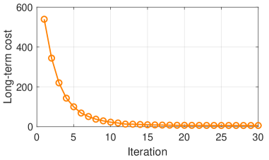
Figure 2: The long-term cost $J_{i}$ converges within 30 iterations.

By Assumption 2, the penalty factor should satisfy $\lambda I-\alpha E^{\top}PE>0$, which in our experiments is $\lambda>0.22$. For demonstration, we select the penalty factor to $\lambda=0.9$ and apply Algorithm 1 to learn a minimax controller. We select the long-term cost at the $i$-th iteration

$$J_{i}=\sum_{k=0}^{M-1}\alpha^{k}((x_{k}^{i})^{\top}Qx_{k}^{i}+(u_{k}^{i})^{\top}Ru_{k}^{i}-\lambda\|w_{k}^{i}-\bar{w}\|^{2})$$

as an indicator for convergence, where $u_{k}^{i}=K_{i}x_{k}^{i}+r_{i}$ and $w_{k}^{i}=L_{i}x_{k}^{i}+l_{i}$ are the pair of optimal solutions at the $i$-th iteration. The result is displayed in Fig. 2. As indicated by Theorem 5, $J_{i}$ converges exponentially, which implies that the Algorithm 1 returns an optimal Q-function.

5 Conclusion

We have proposed a Q-learning algorithm with convergence guarantees to learn a minimax controller with robustness to disturbance distribution errors. Recent years have witnessed the tremendous success in the policy gradient methods, which can be used to solve the zero-sum game (Zhang et al., 2019). We shall study this topic in the future work.

References

• (1)
• Abdullah et al. (2019) Abdullah, M. A., Ren, H., Ammar, H. B., Milenkovic, V., Luo, R., Zhang, M. & Wang, J. (2019), ‘Wasserstein robust reinforcement learning’, arXiv preprint arXiv:1907.13196 .
• Al-Tamimi et al. (2007) Al-Tamimi, A., Lewis, F. L. & Abu-Khalaf, M. (2007), ‘Model-free Q-learning designs for linear discrete-time zero-sum games with application to $\mathcal{H}_{\infty}$ control’, Automatica 43(3), 473–481.
• Åström (2012) Åström, K. J. (2012), Introduction to stochastic control theory, Courier Corporation.
• Başar & Bernhard (2008) Başar, T. & Bernhard, P. (2008), $\mathcal{H}_{\infty}$ optimal control and related minimax design problems: a dynamic game approach, Springer Science & Business Media.
• Chen & Paschalidis (2020) Chen, R. & Paschalidis, I. C. (2020), ‘Distributionally robust learning’, Foundations and Trends® in Optimization 4(1-2), 1–243.
• Gao & Kleywegt (2022) Gao, R. & Kleywegt, A. J. (2022), ‘Distributionally robust stochastic optimization with wasserstein distance’, Mathematics of Operations Research .
• Kim & Yang (2020) Kim, K. & Yang, I. (2020), Minimax control of ambiguous linear stochastic systems using the wasserstein metric, in ‘59th IEEE Conference on Decision and Control (CDC)’, pp. 1777–1784.
• Kim & Yang (2021) Kim, K. & Yang, I. (2021), ‘Distributional robustness in minimax linear quadratic control with wasserstein distance’, arXiv preprint arXiv:2102.12715 .
• Lillicrap et al. (2016) Lillicrap, T. P., Hunt, J. J., Pritzel, A., Heess, N., Erez, T., Tassa, Y., Silver, D. & Wierstra, D. (2016), Continuous control with deep reinforcement learning., in ‘International Conference on Learning Representations’.
• Nilim & El Ghaoui (2005) Nilim, A. & El Ghaoui, L. (2005), ‘Robust control of markov decision processes with uncertain transition matrices’, Operations Research 53(5), 780–798.
• Pinto et al. (2017) Pinto, L., Davidson, J., Sukthankar, R. & Gupta, A. (2017), Robust adversarial reinforcement learning, in ‘International Conference on Machine Learning’, PMLR, pp. 2817–2826.
• Wiesemann et al. (2014) Wiesemann, W., Kuhn, D. & Sim, M. (2014), ‘Distributionally robust convex optimization’, Operations Research 62(6), 1358–1376.
• Yang (2021) Yang, I. (2021), ‘Wasserstein distributionally robust stochastic control: A data-driven approach’, IEEE Transactions on Automatic Control 66(8), 3863–3870.
• Zhang et al. (2019) Zhang, K., Yang, Z. & Basar, T. (2019), Policy optimization provably converges to nash equilibria in zero-sum linear quadratic games, in ‘Advances in Neural Information Processing Systems’, pp. 11598–11610.