Vokenization: Improving Language Understanding with
Contextualized, Visual-Grounded Supervision

Abstract

Humans learn language by listening, speaking, writing, reading, and also, via interaction with the multimodal real world. Existing language pre-training frameworks show the effectiveness of text-only self-supervision while we explore the idea of a visually-supervised language model in this paper. We find that the main reason hindering this exploration is the large divergence in magnitude and distributions between the visually-grounded language datasets and pure-language corpora. Therefore, we develop a technique named “vokenization” that extrapolates multimodal alignments to language-only data by contextually mapping language tokens to their related images (which we call “vokens”). The “vokenizer” is trained on relatively small image captioning datasets and we then apply it to generate vokens for large language corpora. Trained with these contextually generated vokens, our visually-supervised language models show consistent improvements over self-supervised alternatives on multiple pure-language tasks such as GLUE, SQuAD, and SWAG.

1 Introduction

Most humans learn language understanding from multiple modalities rather than only from the text and audio, especially using the visual modality. As claimed in Bloom (2002), visual pointing is an essential step for most children to learn meanings of words. However, existing language pre-training frameworks are driven by contextual learning which only takes the language context as self-supervision. For example, word2vec Mikolov et al. (2013) takes surrounding bag-of-words; ELMo Peters et al. (2018) and GPT Radford et al. (2018) take succeeding contexts; and BERT Devlin et al. (2019) takes randomly masked tokens. Although these self-supervised frameworks have achieved strong progress towards understanding human language, they did not borrow grounding information from the external visual world (see related motivations in recent work by Bender and Koller (2020) and Bisk et al. (2020)).

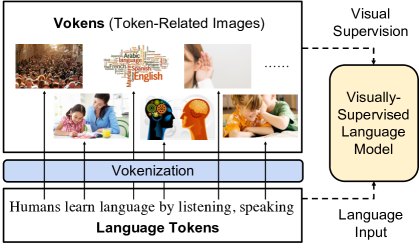
Figure 1: We visually supervise the language model with token-related images. We call these images vokens (visualized tokens) and develop a vokenization process to contextually generate them.

In this paper, we introduce the visually-supervised language model that simulates human language learning with visual pointing Bloom (2002). As shown in Fig. 1, this model takes language tokens as input and uses token-related images as visual supervision. We name these images as vokens (i.e., visualized tokens), since they act as visualizations of the corresponding tokens. Assuming that a large aligned token-voken dataset exists, the model could learn from these vokens via voken-prediction tasks.

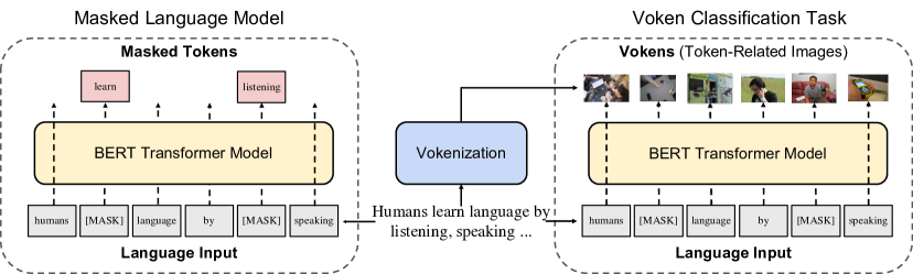
Figure 2: Illustration of the BERT transformer model trained with a visually-supervised language model with two objectives: masked language model (on the left) and voken classification (on the right). The first objective (used in original BERT pre-training) predicts the masked tokens as self-supervision while the second objective predicts the corresponding vokens (contextually generated by our vokenization process) as external visual supervision. Since the inputs are the same, we optimize the two objectives simultaneously and share the model weights.

Unfortunately, such an aligned token-voken dataset is currently unavailable and hence there are two main challenges in creating it from visually-grounded language datasets. First, there is a large discrepancy between visually-grounded language (which provides innate visual grounding supervision) and other types of natural language. For example, about 120M tokens are available in visually-grounded language datasets Tan and Bansal (2019); Chen et al. (2019), which is far less compared to the 3,300M tokens in BERT training data and 220B tokens in T5 Raffel et al. (2019). Grounded language also prefers short and instructive descriptions, and thus has different distributions of sentence lengths and active words to other language types. Second, most of the words in natural language are not visually grounded, hence this challenges the premise in creating visual supervision. With an approximate estimation, the ratio of grounded tokens is only about $28\%$ in English Wikipedia. This low grounding ratio leads to low coverage of visual supervision in previous approaches Frome et al. (2013); Kiela et al. (2018).

To resolve the above two challenges, we propose our vokenization method (as shown in Fig. 1) that contextually maps the tokens to the visualized tokens (i.e., vokens) by retrieval. Instead of directly supervising the language model with visually grounded language datasets (e.g., MS COCO Lin et al. (2014)), we use these relative small datasets to train the vokenization processor (i.e., the vokenizer). We then generate vokens for large language corpora (e.g., English Wikipedia), and our visually-supervised language model will take the input supervision from these large datasets, thus bridging the gap between different data sources, which solves the first challenge. The second challenge of low grounding ratio seems to be an inherent characteristic of language; however, we observe that some non-visually-grounded tokens can be effectively mapped to related images when considering its context, e.g., the abstract word “angry” in the sentence “an angry cat lies on my leg”. This observation is realized by our contextual token-image matching model (defined in Sec. 3.2) inside our vokenization processor, where we map tokens to images by viewing the sentence as the context.

Using our proposed vokenizer with a contextualized token-image matching model, we generate vokens for English Wikipedia. Supervised by these generated vokens, we show consistent improvements upon a BERT model on several diverse NLP tasks such as GLUE Wang et al. (2019), SQuAD Rajpurkar et al. (2016), and SWAG Zellers et al. (2018). We also show the transferability of our vokens to other frameworks (i.e., RoBERTa).

Dataset	# of Tokens	# of Sents	Vocab. Size	Tokens #/ Sent.	1-Gram JSD	2-Gram JSD	Grounding Ratio
MS COCO	7.0M	0.6M	9K	11.8	0.15	0.27	54.8%
VG	29.2M	5.3M	13K	5.5	0.16	0.28	57.6%
CC	29.9M	2.8M	17K	10.7	0.09	0.20	41.7%
Wiki103	111M	4.2M	29K	26.5	0.01	0.05	26.6%
Eng Wiki	2889M	120M	29K	24.1	0.00	0.00	27.7%
CNN/DM	294M	10.9M	28K	26.9	0.04	0.10	28.3%

Table 1: Statistics of image-captioning dataset and other natural language corpora. VG, CC, Eng Wiki, and CNN/DM denote Visual Genome, Conceptual Captions, English Wikipedia, and CNN/Daily Mail, respectively. JSD represents Jensen–Shannon divergence to the English Wikipedia corpus. A large discrepancy exists between the visually grounded captioning and general language corpora.

2 Visually-Supervised Language Models

Contextual language representation learning is driven by self-supervision without considering explicit connections (grounding) to the external world. In this section, we illustrate the idea of a visually-supervised language model and discuss the challenges of creating its visual supervision.

2.1 Vokens: Visualized Tokens

To provide visual supervision to the language model, we assume a text corpus where each token is aligned with a related image (although these voken annotations currently do not exist, we will try to generate vokens next in Sec. 3 by the vokenization process). Hence, these images could be considered as visualizations of tokens and we name them as ‘vokens’. Based on these vokens, we propose a new pre-training task for language: voken classification.

2.2 The Voken-Classification Task

Most language backbone models (e.g., ELMo Peters et al. (2018), GPT Radford et al. (2018), BERT Devlin et al. (2019)) output a localized feature representation $\{\bm{h}_{i}\}$ for each token in a sentence $s=\{w_{i}\}$. Thus it allows adding a token-level classification task without modifying the model architecture. Suppose the vokens come from a finite set $\mathbb{X}$, we convert the hidden output $\bm{h}_{i}$ to a probability distribution $p_{i}$ with a linear layer and a softmax layer, then the voken classification loss is the negative log probability of all corresponding vokens:

$$\bm{h}_{1},\bm{h}_{2},\ldots,\bm{h}_{l} =\mathrm{lm}(w_{1},w_{2},\ldots,w_{l})$$

$$p_{i}(v\mid s) =\mathrm{softmax}_{v}\{W\,\bm{h}_{i}+b\}$$

$$\mathcal{L}_{\textsc{voken-cls}}(s) =-\sum_{i=1}^{l}\log p_{i}\left(v(w_{i};s)\mid s\right)$$

This task could be easily integrated into current language pre-training frameworks, and we next show an example.

Example: Visually-Supervised BERT

Fig. 2 shows an example realization of the voken-classification task that provides visual supervision to BERT Devlin et al. (2019). The original BERT pre-training mainly relies on the task of masked language model (illustrated on the left side of Fig. 2): tokens are randomly masked and the model needs to predict these missing tokens from language context. For simplicity, we use $s$ and $\hat{s}$ to denote the set of tokens and masked tokens, separately. The unmasked tokens are the set difference $s\setminus\hat{s}$. Suppose $q_{i}$ is the conditional probability distribution of the $i$-th token, the Masked Language Model (MLM) loss is the negative log-likelihood of the masked tokens:

$$\mathcal{L}_{\textsc{mlm}}(s,\hat{s})=-\sum_{w_{i}\in\hat{s}}\log q_{i}\left(w_{i}\mid s\setminus\hat{s}\right)$$

Without changing the model and model’s inputs, we calculate the voken-classification loss for all tokens (illustrated on the right side of Fig. 2):

$$\mathcal{L}_{\textsc{voken-cls}}(s,\hat{s})=-\sum_{w_{i}\in s}\log p_{i}\left(v(w_{i};s)\mid s\setminus\hat{s}\right)$$

The visually-supervised masked language model takes the sum of these two losses with a ratio $\lambda$.

$$\mathcal{L}_{\textsc{vlm}}(s,\hat{s})=\mathcal{L}_{\textsc{voken-cls}}(s,\hat{s})+\lambda\mathcal{L}_{\textsc{mlm}}(s,\hat{s})$$ (1)

2.3 Two Challenges in Creating Vokens

Previous sections illustrate the potential external supervision by assuming the existence of vokens. However, we are currently lacking the dense annotations from tokens to images. The most similar concept to vokens is phrase localization (e.g., in Flickr30K entities Young et al. (2014); Plummer et al. (2017)). Because the process of collecting phrase localization is costly, the coverage and the amount of annotations cannot meet our requirements. Apart from phrase localization, the most promising data source is image captioning datasets with sentence-to-image mappings (or discovered from multimodal documents, as in Hessel et al. (2019)). Image captions belong to a specific type of language called grounded language Roy and Pentland (2002); Hermann et al. (2017), which has an explicit grounding to external existence or physical actions. However, grounded language has a large discrepancy to other types of natural language (e.g., News, Wiki, and Textbooks). To illustrate this, we list key statistics of three image-captioning dataset (i.e., MS COCO Lin et al. (2014), Visual Genome Krishna et al. (2017), and Conceptual Captions Sharma et al. (2018)) and three language corpora of other language types (i.e., Wiki103 Merity et al. (2017), English Wiki, and CNN/Daily Mail See et al. (2017)) in Table 1. This discrepancy between grounded language and other types of natural language leads to two challenges:

A. Different Distributions between Grounded Language and Other Natural Language Corpora.  Sentences belonging to grounded language are usually short and informative, e.g., the average sentence length in MS COCO is $11.8$, which is much shorter than the average sentence length of $24.1$ in English Wiki. The vocabulary of MS COCO only covers around one-third of token types Smith (2019) in English Wiki. There is also a large divergence of the 1-Gram and 2-Gram distributions (measured by Jensen–Shannon divergence) between grounded language dataset and the English Wikipedia. Lastly, the amount of tokens in grounded language corpora are also orders of magnitude smaller than commonly-used Wikipedia.

B. Low Grounding Ratio in Natural Language.  The grounding ratio is defined as the percentage of visually grounded tokens in the dataset. Visually grounded tokens (e.g., concrete nouns) are the token types that are naturally related to specific visual contents (e.g., ‘cat’, ‘cake’, ‘clock’). Since a precise list of such token types is hard to define, we thus estimate the grounding ratio based on existing grounded language corpora. Specifically, we consider a token type with more than $100$ occurrences in MS COCO (after removing all stop words) as visually-grounded. A sample of these token types could be found in the Appendix. As shown in the last column of Table 1, the grounding ratio of English Wiki is $27.7\%$, which is almost half of that in Visual Genome.

To address these two challenges, we propose a vokenizer with contextual token-image matching models next in Sec. 3.

3 Vokenization

In the previous section, we discuss the potential of using vokens (i.e., visualized tokens) as visual supervision to the language model, and also demonstrate the large gap between currently available resources (i.e., annotated dataset) and the desired requirements. Hence, in this section, we develop a framework that can generate vokens. As shown in Fig. 2, the general idea is that we learn a “vokenizer” from image-captioning dataset and use it to annotate large language corpora (i.e., English Wiki), thus bridging the gap between grounded language and other types of natural language. We start by illustrating the vokenization process and then describe how we implement it.

3.1 The Vokenization Process

As shown in Fig. 1 and Fig. 2, vokenization is the process to assign each token $w_{i}$ in a sentence $s=(w_{1},w_{2},\ldots,w_{l})$ with a relevant image $v(w_{i};s)$. We call this image $v(w_{i};s)$ as a ‘voken’ (visualized token). Instead of creating this image with generative models, we retrieve an image from a set of images $\mathbb{X}=\{x_{1},x_{2},\ldots,x_{n}\}$ regarding a token-image-relevance scoring function $r_{\theta}(w_{i},x;s)$. This scoring function $r_{\theta}(w_{i},x;s)$, parameterized by $\theta$, measures the relevance between the token $w_{i}$ in the sentence $s$ and the image $x$. We here assume that the optimal parameter of this function is $\theta^{*}$ and will discuss the details of formulations later. The voken $v(w_{i};s)$ related to a token $w_{i}$ in the sentence $s$ is realized as the image $x\in\mathbb{X}$ that maximizes their relevance score $r_{\theta^{*}}$:

$$v(w_{i};s)=\arg\max\nolimits_{x\in\mathbb{V}}\,r_{{\theta}^{*}}(w_{i},x;s)$$

Since the image set $\mathbb{X}$ indeed builds a finite vocabulary for vokens, we could utilize the voken-classification task (formulated in Sec. 2.2) to visually supervise the language model training. We next talk about the detailed implementation of this vokenization process.

3.2 Contextual Token-Image Matching Model

Lying in the core of the vokenization process is a contextual token-image matching model. The model takes a sentence $s$ and an image $x$ as input, and the sentence $s$ is composed of a sequence of tokens $\{w_{1},w_{2},\ldots,w_{l}\}$. The output $r_{\theta}(w_{i},x;s)$ is the relevance score between the token $w_{i}\in s$ and the image $x$ while considering the whole sentence $s$ as a context.

Modeling

To model the relevance score function $r_{\theta}(w_{i},x;s)$, we factorize it as an inner product of the language feature representation $\bm{f}_{\theta}(w_{i};s)$ and the visual feature representation $\bm{g}_{\theta}(x)$:

$$r_{\theta}(w_{i},x;s)=\bm{f}_{\theta}(w_{i};s)^{\intercal}\bm{g}_{\theta}(x)$$

These two feature representations are generated by language and visual encoders respectively. The language encoder first uses a pre-trained $\text{BERT}_{\text{BASE}}$ Devlin et al. (2019) model to contextually embed the discrete tokens $\{w_{i}\}$ into hidden-output vectors $\{\bm{h}_{i}\}$:

$$\bm{h}_{1},\bm{h}_{2},\ldots,\bm{h}_{l}=\mathit{bert}(w_{1},w_{2},\ldots,w_{l})$$

Then we apply a multi-layer perceptron (MLP) $\mathit{w\mbox{\_}mlp}_{\theta}$ to down project the hidden output $\bm{h}_{i}$. In order to simplify the retrieval process in Sec. 3.1, the final language features are normalized to norm-1 vectors by dividing their Euclidean norms:

$$\bm{f}_{\theta}(w_{i};s)=\frac{\mathit{w\mbox{\_}mlp}_{\theta}(\bm{h}_{i})}{\|\mathit{w\mbox{\_}mlp}_{\theta}(\bm{h}_{i})\|}$$

On the other side, the visual encoder first extracts the visual embedding $e$ from a pre-trained ResNeXt Xie et al. (2017). Similar to the language encoder, an MLP layer $\mathit{x\mbox{\_}mlp}_{\theta}$ and an L2-normalization layer are applied subsequently:

$$\bm{e} =\mathrm{ResNeXt}(x)$$

$$\bm{g}_{\theta}(x) =\frac{\mathit{x\mbox{\_}mlp}_{\theta}(\bm{e})}{\|\mathit{x\mbox{\_}mlp}_{\theta}(\bm{e})\|}$$

Training

Since the dense annotations from tokens to images are lacking and hard to generate (illustrated in Sec. 2.3), we thus alternatively train the token-image matching model from weak supervision in image-captioning datasets (e.g., MS COCO Lin et al. (2014)). These datasets are comprised of sentence-image pairs $\{(s_{k},x_{k})\}$ where the sentence $s_{k}$ describes the visual content in image $x_{k}$. To build alignments between tokens and images, we pair all tokens in a sentence $s_{k}$ with the image $x_{k}$. The model is then optimized by maximizing the relevance score of these aligned token-image pairs over unaligned pairs.

Without loss of generality, assuming $(s,x)$ is an image-captioning data point, we randomly sample another image $x^{\prime}$ with the condition $x^{\prime}\neq x$. We then use hinge loss to optimize the weight $\theta$ so that the score of the positive token-image pair $r_{\theta}(w_{i},x;s)$ aims to be larger than the negative pair $r_{\theta}(w_{i},x^{\prime};s)$ by at least a margin $M$.

$$\vspace{-5pt}\mathcal{L}_{\theta}(s,x,x^{\prime})=\sum_{i=1}^{l}\max\{0,M -r_{\theta}(w_{i},x;s)$$

$$+r_{\theta}(w_{i},x^{\prime};s)\}$$

Intuitively, minimizing this hinge loss $\max\{0,$ $M-\mathit{pos}+\mathit{neg}\}$ will try to increase the score of the positive pair and decrease the score of the negative pair when the score difference is smaller than the margin $M$. Otherwise (if the difference is $\geq$ margin $M$), the two scores remain unchanged.

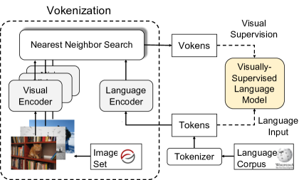
Figure 3: Implementation of our vokenization process. For the tokens in language corpora, we contextually retrieved images (with nearest neighbor search) from the image set as vokens. These generated vokens are then used as the visual supervision to the language model.

Inference

Given that the relevance score is factorized as the inner product of feature representations $\bm{f}_{\theta}(w_{i};s)$ and $\bm{g}_{\theta}(v)$, the retrieval problem in Sec. 3.1 could be formulated as Maximum Inner Product Search Mussmann and Ermon (2016)). Moreover, since the vectors are norm-1, the vector with the maximum inner product is identical to the closest vector in the Euclidean space (i.e., Nearest Neighbor Knuth (1973)). We illustrate the detailed implementation in Fig. 3.

3.3 Revokenization

A constraint of the vokenization process in Sec. 3.1 is that the vokens depend on the actual tokenizer of the language encoder in Sec. 3.2. Since different frameworks utilize a various range of tokenizers, this constraint limits the transferability of vokens between different frameworks. Instead of binding our vokenizer to a specific pre-training framework (e.g., BERT), we want to enable its extensibility to other frameworks (e.g., RoBERTa). Thus, we introduce a “revokenization” technique to address this limitation.

Given two different tokenizers $T_{1}$ and $T_{2}$, they tokenize a sentence $s$ into two different sequences of tokens: $T_{1}(s)=\left(w_{1},w_{2},\ldots,w_{l}\right)$ and $T_{2}(s)=\left(u_{1},u_{2},\ldots,u_{m}\right)$. Without loss of generality, assuming the vokenizer is built based on the first tokenizer $T_{1}$, the standard vokenization process will generate a sequence of vokens $\{v(w_{i};s)\}_{i=1}^{l}$ which are one-to-one aligned with the tokens $\{w_{i}\}_{i=1}^{l}$. Our goal is to transfer these $w$-related vokens to the $u$-related vokens generated by $T_{2}$. We adapt the idea of “nearest neighbor algorithm” Altman (1992) here. For a given token $u_{j}$, among all $w$’s, we select the one that overlaps the most with $u_{j}$ and record it as $w_{\mathit{ind}(j)}$. The voken for $u_{j}$ is defined as the voken for its “nearest neighbor” $w_{\mathit{ind}(j)}$:

$$v(u_{j};s):=v(w_{\mathit{ind}(j)};s)$$

$$\mathit{ind}(j) =\arg\max\nolimits_{i=1}^{l}\mathrm{overlap}(w_{i},u_{j})\vspace{-5pt}$$

The overlapping of two tokens are further quantified by the intersection-over-union (i.e., Jaccard index, defined as $\mathrm{IoU}(A,B)\mbox{=}\frac{|A\cap B|}{|A\cup B|}$) of their ranges in the raw sentence $s$.

Method	SST-2	QNLI	QQP	MNLI	SQuAD v1.1	SQuAD v2.0	SWAG	Avg.
$\text{BERT}_{\text{6L/512H}}$	88.0	85.2	87.1	77.9	71.3/80.2	57.2/60.8	56.2	75.6
$\text{BERT}_{\text{6L/512H}}$ + Voken-cls	89.7	85.0	87.3	78.6	71.5/80.2	61.3/64.6	58.2	76.8
$\text{BERT}_{\text{12L/768H}}$	89.3	87.9	83.2	79.4	77.0/85.3	67.7/71.1	65.7	79.4
$\text{BERT}_{\text{12L/768H}}$ + Voken-cls	92.2	88.6	88.6	82.6	78.8/86.7	68.1/71.2	70.6	82.1
$\text{RoBERTa}_{\text{\,6L/512H}}$	87.8	82.4	85.2	73.1	50.9/61.9	49.6/52.7	55.1	70.2
$\text{RoBERTa}_{\text{\,6L/512H}}$ + Voken-cls	87.8	85.1	85.3	76.5	55.0/66.4	50.9/54.1	60.0	72.6
$\text{RoBERTa}_{\text{\,12L/768H}}$	89.2	87.5	86.2	79.0	70.2/79.9	59.2/63.1	65.2	77.6
$\text{RoBERTa}_{\text{\,12L/768H}}$ + Voken-cls	90.5	89.2	87.8	81.0	73.0/82.5	65.9/69.3	70.4	80.6

Table 2: Fine-tuning results of different pre-trained models w/ or w/o the voken classification task (denoted as “Voken-cls”). SQuAD results are “exact match”/“F1”. The results which significantly outperform the second-best ones are marked in bold. The averages of metrics (denoted as “Avg.”) show improvement from voken supervisions.

4 Experimental Setups and Results

4.1 Pre-training Data and Fine-tuning Tasks

We train our model on English Wikipedia  and its featured subset Wiki103 Merity et al. (2017). We use our vokenizer to generate vokens for these two datasets as well. The pre-trained models are then fine-tuned on GLUE Wang et al. (2019), SQuAD Rajpurkar et al. (2016, 2018), and SWAG Zellers et al. (2018) to assess the pre-training performance. Since some smaller tasks in GLUE are reported as unstable Dodge et al. (2020), recent papers (e.g., Li et al. (2020b)) only report on selected tasks. We follow this trend and evaluate on the four largest datasets (i.e., SST-2 Socher et al. (2013), QNLI Rajpurkar et al. (2016), QQP Iyer et al. (2017), MNLI Williams et al. (2018))..

4.2 Implementation Details

We train our contextual token-image matching model (in Sec. 3.2) on MS COCO image captioning dataset for $20$ epochs. The concatenation of the last 4 layers of BERT outputs and $\mathrm{ResNeXt\mbox{-}101\mbox{-}32x8d}$ features are used as language hidden states and visual embedding, respectively. Both multi-layer perceptrons $\mathit{w\mbox{\_}mlp}_{\theta}$ and $\mathit{x\mbox{\_}mlp}_{\theta}$ have two fully-connected layers with $256$-dimensional intermediate outputs (followed by ReLU activation) and $64$-dimensional final outputs. The two backbone models BERT Devlin et al. (2019) and ResNeXt Xie et al. (2017) are not fine-tuned. We set the hinge loss margin $M$ to $0.5$. During the vokenization process of English Wikipedia and Wiki103, we use the faiss Johnson et al. (2019) library to speed up the nearest neighbor search. The vokens are retrieved from the Visual Genome images that are not used in MS COCO. We fix a voken size of $50000$.

When pre-training the model on pure language corpus, we unify the training protocols to avoid possible side effects. We follow previous works to conduct two simplifications: 1. Removing the next-sentence-prediction task Liu et al. (2019) 2. Using fixed sequence length Conneau et al. (2020) of $128$. We take the $12$-layer $\text{BERT}_{\text{BASE}}$ model of $768$ hidden dimensions and train it on English Wikipedia for $200$K steps from scratch. We also take a reduced $6$-layer model and train it on Wiki103 for $40$ epochs ($160$K steps) because this reduced model could not fit the full English Wikipedia dataset.

Since we only use the vokens in the supervision, the voken-classification task does not bring additional parameters to the language model but needs more computations. We thus adjust the training steps for pure masked-language-model (MLM) training accordingly for a fair comparison. The loss ratio $\lambda\mbox{=}1.0$ in Eqn. 1 is not tuned because of limited budget. All pre-training processes take batch sizes of $256$ and learning rates of $2e\mbox{-}4$. For fine-tuning tasks, we report the results on the validation sets. We train $3$ epochs with a learning rate of $1e\mbox{-}4$ and a batch-size of $32$ for all tasks in GLUE. The hyper-parameters for SQuAD, SWAG are borrowed from BERT.

Model	Init. with BERT?	Diff. to BERT Weight	SST-2	QNLI	QQP	MNLI
ViLBERT Lu et al. (2019)	Yes	0.0e-3	90.3	89.6	88.4	82.4
VL-BERT Su et al. (2020)	Yes	6.4e-3	90.1	89.5	88.6	82.9
VisualBERT Li et al. (2019)	Yes	6.5e-3	90.3	88.9	88.4	82.4
Oscar Li et al. (2020a)	Yes	41.6e-3	87.3	50.5	86.6	77.3
LXMERT Tan and Bansal (2019)	No	42.0e-3	82.4	50.5	79.8	31.8
$\text{BERT}_{\text{BASE}}$ Devlin et al. (2019)	-	0.0e-3	90.3	89.6	88.4	82.4
$\text{BERT}_{\text{BASE}}$ + Weight Noise	-	6.5e-3	89.9	89.9	88.4	82.3

Table 3: Results of vision-and-language pre-trained models on GLUE tasks. We also provide BERT models w/ and w/o weight noise as baselines.

Pre-trained on	SST-2	QNLI	QQP	MNLI
MS COCO	83.7	60.6	82.1	69.3
Wiki103*	85.8	77.9	84.8	73.9
No Pre-train	77.1	50.5	31.6	31.8

Table 4: Results of BERT models pre-trained on captions in MS COCO and a reduced version of Wiki103 dataset (denoted as Wiki103*). Models without pre-training are taken as a baseline.

4.3 Results

As reported in Table 2, we fine-tune the pre-trained models on different natural-language tasks. The models are either pre-trained with masked language model (e.g., “$\text{BERT}_{\text{6L/512H}}$”) or pre-trained with masked language model with an additional voken-classification task (e.g., “$\text{BERT}_{\text{6L/512H}}$+Voken-cls”) following Eqn. 1. The default metric is accuracy. Following Wang et al. (2019), we report the average of F1 and accuracy for QQP. For SQuAD, we report the exact matching and F1 score respectively. We also compute macro-averages for evaluated tasks (denoted as “Avg.” in the last column) as a general indicator. Although the different architectures of models (i.e., 6L/512H and 12L/768H) affect the fine-tuning results, the voken-classification task consistently improves the downstream tasks’ performance and achieves large average gains. We also show the transferability of our vokenizer to the RoBERTa model and observe the same phenomenon as that in BERT.

Method	Retrieval	Supervision	SST-2	QNLI	QQP	MNLI
SentLabel	Sent-level	Sent-level	88.3	86.1	86.9	78.0
Propagated	Sent-level	Token-level	88.9	87.9	88.1	80.2
Term Frequency	Token-level	Token-level	89.0	86.9	85.5	79.8
Vokens	Contextual Token-level	Token-level	92.2	88.6	88.6	82.6

Table 5: Comparisons of sentence-level (denoted as “Sent-level”) and token-level approaches. Token-level approaches outperform the sentence-level approaches from both retrieval-method and supervision perspective.

5 Analysis

5.1 Limit of Visually-Grounded Language

In Sec. 2.3, we illustrated the differences between (visually-)grounded-language datasets and other natural-language corpora by demonstrating their contrasting statistics. In this section, we study the models trained with grounded language and show their ineffectiveness on pure-language tasks. We first investigate vision-and-language pre-training frameworks, which succeed on multimodal tasks. As shown in Table 3, when fine-tuning them on pure-language tasks, the results are generally lower than the pre-trained BERT model. Although these frameworks are different in multiple ways, the only remarkable factor to the fine-tuning results is the BERT-weight initialization. Moreover, we also show that these models are similar to a BERT model with a random weight noise of the same magnitude. We thus claim that vision-and-language pre-training on visually-grounded language dataset currently might not help the pure-language tasks. Note that the BERT results in Table 2 are not fairly comparable to the results in Table 3 because the original BERT model Devlin et al. (2019) also uses Toronto Books Corpus Zhu et al. (2015). Unfortunately, this dataset is not publicly available and hence we exclude it. According to Raffel et al. (2019), the exclusion of Toronto Books Corpus downgrades the results and we observe the same tendency here (comparing $\text{BERT}_{\text{12L/768H}}$ in Table 2 and $\text{BERT}_{\text{BASE}}$ in Table 3).

Besides these existing models, we next investigate the BERT models trained with masked language model on grounded language data (i.e., MS COCO). A control experiment is built by shrinking the Wiki103 to the same token amount as MS COCO. We also provide the BERT model trained from scratch as a baseline. As shown in Table 4, the model trained with MS COCO is significantly worse than the model trained with Wiki103 on all downstream tasks. The reason might be the large discrepancy between visually-grounded language and other types of language as shown in Sec. 2.3.

5.2 Token-Level vs. Sentence-Level Approaches

In Sec. 1, we stated the drawbacks of the purely sentence-level and token-level approaches, then introduce the contextual token-level approach (i.e., the contextual token-image matching model in Sec. 3.2) which combines these two approaches. In this section, we demonstrate a careful comparison between our vokenization process and the other two approaches from two perspectives: the retrieval methods and the supervision types. Experiments are conducted with the same hyper-parameters and dataset as “$\text{BERT}_{\text{12L/768H}}$+Voken-cls” in Table 2.

Sentence-Level Retrieval

To conduct sentence-level retrieval, we first adapt the contextual token-image matching model in Sec. 3.2 to a sentence-image matching model (details in Appendix). We then retrieve a related image for each sentence. As shown in Table 5, these retrieved images are used as two kinds of supervisions by putting classifiers at different places: in the row “SentLabel”, we provide sentence-level supervision by using the classifier to predict the label for the whole sentence (similar to the BERT’s “next-sentence prediction” (NSP) task); and in the row “Propagated”, we provide token-level supervision by propagating sentence-level labels to all tokens in the sentences, and apply the classifier at each token (similar to our voken-classification task). The results of both kinds of supervisions are lower than our proposed vokens (in the row “Vokens”). One possible reason for these lower results is that finding an image that conveys the meaning of the whole sentence is hard. We also find that dense token-level supervision also outperforms the sentence-level supervision.

Token-level Retrieval

Our proposed vokenization process is viewed as contextual token-level retrieval, which grounds tokens with whole sentences as context. We here consider a purely token-level retrieval method regarding term frequencies. The term frequency $\mathit{tf}(\mathit{tok},x_{i})$ Manning et al. (2008) is calculated based on the occurrence $\#(\mathit{tok},x_{i})$ of the token $\mathit{tok}$ in the image $x_{i}$’s captions.

$$\vspace{-5pt}\mathit{tf}(\mathit{tok},x_{i})=\frac{\#(\mathit{tok},x_{i})}{\sum_{\mathit{tok}^{\prime}}\#(\mathit{tok}^{\prime},x_{i})}$$

We then convert this term frequency to the conditional distribution via Boltzmann distribution:

$$p(x_{i}\mid\mathit{tok})=\frac{\exp{\left(\mathit{tf}(\mathit{tok},x_{i})/\gamma\right)}}{\sum_{x^{\prime}}\exp{\left(\mathit{tf}(\mathit{tok},x^{\prime})/\gamma\right)}}$$

where $\gamma$ is temperature. We stochastically map the tokens to images with this conditional distribution $p(x_{i}\mid\mathit{tok})$. The results trained with these special vokens are shown in Table 5 as “Term Frequency”. Overall, token-level supervision is still better than the sentence-level supervision (as in the row “SentLabel”). However, among the models trained with token-level supervision, this token-level retrieval method neglects the contextual information thus is worse compared with sentence-level (in the row “Propagated”) and contextual token-level retrieval methods (in the row “Voken”) .

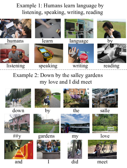
Figure 4: Visualization of model-generated vokens. Example 1 takes the leading sentence of this paper while Examples 2 takes Yeats’s poet.

5.3 Visualization of Vokens

In Fig. 4, we visualize our generated vokens. The first example takes the leading sentence in our paper (without commas), which is also used in the imaginary example in Fig. 1. We also vokenize another sentence from William Yeats’s poet “Down by the Salley Gardens” in Fig. 4. Although the vokenizer is trained on image-captioning datasets without localizing token-to-image annotations, the vokenizer shows a strong selectivity: different images are selected w.r.t the tokens. The contextual token-level retrieval could also disambiguate certain tokens (e.g., “down” in Example 2) with the help of its context. When the unique related image is hard to define, our vokenizer aims to ground the non-concrete tokens (e.g., “by”/“and”/“the”) to relevant images: the voken for the token “by” in Example 2 (of Fig. 4) is better aligned with the [centering token, context] pair than the voken for the same token “by” in Example 1. This related visual information helps understand the language and leads to the improvement in Table 2. On the other hand, some tokens are not faithfully grounded (e.g., “writing” in Example 1) and we also observe a shift in alignment (e.g., the relevant image for the phrase “my love” in Example 2 is aligned to “my” instead of “love”). These misalignments are possibly caused by the limitations of sentence-image weak supervision in our training data since the strong token-image annotations are not available.

6 Related Work

Language (Model) Pre-training

Language pre-training has moved from token-level pre-training Mikolov et al. (2013); Pennington et al. (2014) to sentence-level pre-training Le and Mikolov (2014); Kiros et al. (2015); Conneau et al. (2017); Dai and Le (2015). Recently, a set of works Peters et al. (2018); Radford et al. (2018); Devlin et al. (2019); Yang et al. (2019); Liu et al. (2019); Clark et al. (2019); Lan et al. (2019) bring back token-level supervision with contextual language encoders (e.g., based on an LSTM Hochreiter and Schmidhuber (1997) and Transformers Vaswani et al. (2017)). This tendency inspires the design of our vokenizer in merging previous sentence-level Frome et al. (2013) and token-level Kiela et al. (2018) approaches into a contextual token-level approach.

Vision-and-Language Pre-training

Since language models are trained with self-supervision without knowing the connection to the visual world, vision-and-language pre-training Li et al. (2019); Lu et al. (2019); Tan and Bansal (2019); Chen et al. (2019); Su et al. (2020); Zhou et al. (2020) aims to build joint cross-modal representations and focuses on vision-and-language tasks. Due to particularity of grounded language, these models are not able to improve pure language tasks as shown in Sec. 5.1.

Visually-Aided Language Learning

Previous works use visual information to improve specific language tasks such as coreference resolution Kong et al. (2014), machine translation Elliott et al. (2016); Ive et al. (2019); Wu et al. (2019); Zhang et al. (2020), semantic parsing Christie et al. (2016); Shi et al. (2019); Kojima et al. (2020), and bilingual lexicon learning Kiela et al. (2015); Vulić et al. (2016). Our work has a focus on building a visually-supervised language pre-training frameworks to improve general language understanding. Similar to our work, Frome et al. (2013); Lazaridou et al. (2015); Collell et al. (2017); Kiela et al. (2018); Bordes et al. (2019) aim to improve language representation with visual information; however, most of these works focus on grounded language and hence might suffer from the large discrepancy that we discuss in Sec. 2.3.

7 Conclusion

In this paper, we explored the possibility of utilizing visual supervision to language encoders. In order to overcome the challenges in grounded language, we develop the vokenizer with contextual token-image matching models and use it to vokenize the language corpus. Supervised by these generated vokens, we observe a significant improvement over the purely self-supervised language model on multiple language tasks.

Appendix A Appendices

A.1 Full Implementation Details

We train our contextual token-image matching model (in Sec. 3.1) on MS COCO image captioning dataset for $20$ epochs. The concatenation of the last 4 layers of BERT outputs (following Devlin et al. (2019)) and mean pooling of $\mathrm{ResNeXt\mbox{-}101\mbox{-}32x8d}$ feature maps are used as features for tokens and the images. For both multi-layer perceptrons $\mathit{w\mbox{\_}mlp}_{\theta}$ and $\mathit{x\mbox{\_}mlp}_{\theta}$, we use two fully-connected layers with ReLU activation, where the output dimensions of the two layers are $256$ and $64$, accordingly. We only train the modules marked with $\theta$, i.e., the two backbone models BERT Devlin et al. (2019) and ResNeXt Xie et al. (2017) are not fine-tuned. Since we normalize the features $g(w_{i};s)$ and $f(v)$ to be norm-1 vectors, the relevance score thus takes the range from $[-1,1]$ (from the Cauchy Inequality). The margin $M$ in hinge loss is set to $0.5$.

During the vokenization process, we use the faiss Johnson et al. (2019) library to speed up the nearest neighbor search. The vokenization runs at a speed of 100K tokens / second with 4 Titan V100 GPU. Thus the vokenization of the full Wikipedia is finished in 8 hours. When transferring vokens to other pre-training frameworks, revokenization does not need the GPU computation and runs as fast as the tokenization. The vokens are retrieved from the Visual Genome images which are not used in MS COCO (our training dataset). We take a voken size of $50000$.

When pre-training the model on pure language corpus, we unify the training process to avoid possible side effects from different training protocols. We follow previous work to conduct two simplifications: 1. Removing the next-sentence-prediction task Liu et al. (2019) 2. Using fixed sequence length Conneau et al. (2020) of $128$. We take the $12$-layer $\text{BERT}_{\text{BASE}}$ model of $768$ hidden dimensions and train it on English Wikipedia for $200$K steps from scratch. We also take a reduced $6$-layer model and train it on Wiki103 for $40$ epochs ($160$K steps) from scratch because this reduced model does not fit well on the full Wikipedia dataset. The voken classification task will not bring additional parameters to the language encoder (with $110$M parameters) but need more computations, we thus adjust the training steps for pure masked-language-model (MLM) training for a fair comparison. It results in around $10$% more training steps in pure MLM training. All models take batch sizes of $256$ and a learning rate of $2e\mbox{-}4$.

For fine-tuning tasks, instead of high-cost hyper-parameter sweeping in BERT Devlin et al. (2019), we train $3$ epochs with a learning rate of $1e\mbox{-}4$ and a batch-size of $32$ for all tasks in GLUE. The hyper-parameters for SQuAD and SWAG are borrowed from the BERT paper Devlin et al. (2019). On SQuAD v1.1, we fine-tune for $3$ epochs with a learning rate of $5e\mbox{-}5$ and a batch size of $32$. On SQuAD v2.0, we fine-tune for $2$ epochs with a learning rate of $5e\mbox{-}5$ and a batch size of $48$. On SWAG, we fine-tune for $3$ epochs with a learning rate of $2e\mbox{-}5$ and a batch size of $16$.

The whole framework is built on PyTorch Paszke et al. (2019). The implementations of BERT Devlin et al. (2019) and RoBERTa Liu et al. (2019) are borrowed from PyTorch Transformers Wolf et al. (2019). All evaluation code is from the PyTorch Transformers as well.

A.2 Visually Grounded Token Types

In Sec.2.3, we estimate the visually grounded token types with the help of MS COCO Lin et al. (2014) dataset. We here randomly sample a list of the $2406$ grounded tokens used in the estimation:

photograph, tv, skyscraper, ##bery, wooded, little, stands, away, storage, mound, pouring, rail, ##fl, eye, ##ke, flown, skiing, plate, movie, dead, tossing, couple, racing, dust, licking, palm, stroll, granite, bananas, ledge, chained, monument, individuals, part, exhibit, softball, second, bow, ones, shop, beverages, sandy, sink, angle, ##ia, gives, music, leading, carrying, cookies, reading, faced, ##k, kid, ##ged, playing, winds, saddle, stunts, squat, cabinets, rusty, matching, biker, let, standing, pan, smiles, train, sky, passing, woman, military, feeder, lot, hydra, party, ##l, furnished, rides, strip, ##field, tin, crouched, courtyard, nicely, screens, us, lie, waving, process, equipment, structure, fore, barrier, ##li, beside, toast, catching, tracks

A.3 Maximum Inner Product Search of Norm-1 Vectors

In Sec. 3.1, we normalize the vector to norm-1 vectors thus the Maximum Inner Product Search Mussmann and Ermon (2016) is equivalent to Nearest Neighbor Knuth (1973). Here, we give a simple proof. Suppose $\bm{x}$ and $\bm{y}$ are two vectors of the same dimension, we have

$$\|\bm{x}-\bm{y}\|^{2} =\|\bm{x}\|^{2}+\|\bm{y}\|^{2}-2\bm{x}^{\intercal}\bm{y}$$ (2)

$$=2-2\bm{x}^{\intercal}\bm{y}$$ (3)

Without loss of generality, we assume that there is a unique vector $\bm{\hat{}}{y}\in\mathbb{Y}$ with the maximum inner product and thus

$$\bm{\hat{}}{y}=\arg\min_{x}\|\bm{x}-\bm{y}\|=\arg\max_{x}\bm{x}^{\intercal}\bm{y}$$ (4)

A.4 Details of Sentence-level Retrieval in Analysis

In Sec. 3.1, we consider a contextual token-image matching model with relevance score $r_{\theta}(w,x;s)$. To do sentence-level retrieval, we modify it into a sentence-image matching score $r^{\prime}_{\theta}(x,s)$, and trained it with:

$$\tilde{\mathcal{L}}_{\theta}(s,x,x^{\prime})=\max\{0,M -r^{\prime}_{\theta}(x,s)$$

$$+r^{\prime}_{\theta}(x^{\prime},s)\}$$

The score is also factorized as the dot product of the visual representation and the language representation. However, the language representation here is the sentence embedding (the output for the first token CLS).

We retrieve the image from the same image set $\mathbb{V}$ as vokenization and with the similar Maximum Inner Product Search method:

$$v(s)=\arg\max\nolimits_{x\in\mathbb{V}}\,r^{\prime}_{\theta^{*}}(x,s)$$

These retrieved images as used as the label for the whole sentence.

Voken Type	SST-2	QNLI	QQP	MNLI
Alternative Choices
Random	89.1	87.6	86.6	80.0
Shuffle	89.2	87.3	86.1	80.2
Tokens	89.7	88.8	87.2	80.8
Reference Models
Voken Only	89.8	87.8	86.2	81.7
No Voken	89.3	87.9	83.2	79.4
Voken	92.2	88.6	88.6	82.6

Table 6: Results of different strategies that replace the standard vokenization process.

A.5 Details of Token-level Retrieval in Analysis

In the purely token-level retrieval, we consider the image-captioning sentences as documents and uses traditional IR methods to index them. In order to increase the size of ‘documents’, we aggregate the data from VQA Antol et al. (2015) and Visual Genome Krishna et al. (2017), besides the existing MS COCO Lin et al. (2014) dataset. We also find that the temperature $\gamma\mbox{=}0.01$ gives a reasonable retrieval distribution and use it in our experiment.

A.6 Voken Ablation Studies

In Table 6, we show several approaches that provide alternative voken-like labels to our model.

Random

We replace the vokens with random int from $\{1\ldots\|\mathbb{V}\|\}$, where $\mathbb{V}$ is the “vocabulary” of all vokens.

Shuffle

In order to prove that the order of vokens would affect the results, we shuffle the vokens in each batch and use it as supervision.

Tokens

We here directly use the original tokens in replace of the vokens to see whether any dense supervision could improve the model.

As shown in Table 6, all these results are lower than the reference vokenization strategy.

A.7 Correlations between Improvements and Grounding Ratio

In order to understand where the improvements in the performance are coming from, we also study the correlation between the improvement in results and the visual grounding ratio (approximately measured in the same way as Sec. 2.3). We found that the datasets with higher grounding ratio (e.g., MNLI Williams et al. (2018)) get significant improvements while the datasets (e.g., QNLI Rajpurkar et al. (2016)) with relatively lower grounding ratio do not benefit much from the visual supervision. The dataset MNLI is built from multiple genre (the original SNLI dataset is in fact built from the Flickr images thus has a strong visual connection) and QNLI is purely based on English Wikipedia (The same as SQuAD Rajpurkar et al. (2016)). These correlations may indicate that the visual supervision helps build a better understanding of visually grounded tokens. Although we used contextual information to map non-grounded words to related images through vokenization, the effectiveness of this mapping relies on the original grounding ratio of the data.

References

- Altman (1992) NS Altman. 1992. An introduction to kernel and nearest-neighbor nonparametric regression. The American statistician, 46(3):175–184.
- Antol et al. (2015) Stanislaw Antol, Aishwarya Agrawal, Jiasen Lu, Margaret Mitchell, Dhruv Batra, C Lawrence Zitnick, and Devi Parikh. 2015. Vqa: Visual question answering. In Proceedings of the IEEE international conference on computer vision, pages 2425–2433.
- Bender and Koller (2020) Emily M Bender and Alexander Koller. 2020. Climbing towards nlu: On meaning, form, and understanding in the age of data. In ACL.
- Bisk et al. (2020) Yonatan Bisk, Ari Holtzman, Jesse Thomason, Jacob Andreas, Yoshua Bengio, Joyce Chai, Mirella Lapata, Angeliki Lazaridou, Jonathan May, Aleksandr Nisnevich, Nicolas Pinto, and Joseph Turian. 2020. Experience grounds language. In EMNLP.
- Bloom (2002) Paul Bloom. 2002. How children learn the meanings of words. MIT press.
- Bordes et al. (2019) Patrick Bordes, Éloi Zablocki, Laure Soulier, Benjamin Piwowarski, and Patrick Gallinari. 2019. Incorporating visual semantics into sentence representations within a grounded space. In EMNLP.
- Chen et al. (2019) Yen-Chun Chen, Linjie Li, Licheng Yu, Ahmed El Kholy, Faisal Ahmed, Zhe Gan, Yu Cheng, and Jingjing Liu. 2019. Uniter: Learning universal image-text representations. arXiv preprint arXiv:1909.11740.
- Christie et al. (2016) Gordon Christie, Ankit Laddha, Aishwarya Agrawal, Stanislaw Antol, Yash Goyal, Kevin Kochersberger, and Dhruv Batra. 2016. Resolving language and vision ambiguities together: Joint segmentation & prepositional attachment resolution in captioned scenes. In Proceedings of the 2016 Conference on Empirical Methods in Natural Language Processing, pages 1493–1503.
- Clark et al. (2019) Kevin Clark, Minh-Thang Luong, Quoc V Le, and Christopher D Manning. 2019. Electra: Pre-training text encoders as discriminators rather than generators. In International Conference on Learning Representations.
- Collell et al. (2017) Guillem Collell, Ted Zhang, and Marie-Francine Moens. 2017. Imagined visual representations as multimodal embeddings. In Thirty-First AAAI Conference on Artificial Intelligence.
- Conneau et al. (2020) Alexis Conneau, Kartikay Khandelwal, Naman Goyal, Vishrav Chaudhary, Guillaume Wenzek, Francisco Guzmán, Edouard Grave, Myle Ott, Luke Zettlemoyer, and Veselin Stoyanov. 2020. Unsupervised cross-lingual representation learning at scale. In ACL.
- Conneau et al. (2017) Alexis Conneau, Douwe Kiela, Holger Schwenk, Loïc Barrault, and Antoine Bordes. 2017. Supervised learning of universal sentence representations from natural language inference data. In Proceedings of the 2017 Conference on Empirical Methods in Natural Language Processing, pages 670–680.
- Dai and Le (2015) Andrew M Dai and Quoc V Le. 2015. Semi-supervised sequence learning. In Advances in neural information processing systems, pages 3079–3087.
- Devlin et al. (2019) Jacob Devlin, Ming-Wei Chang, Kenton Lee, and Kristina Toutanova. 2019. Bert: Pre-training of deep bidirectional transformers for language understanding. In Proceedings of the 2019 Conference of the North American Chapter of the Association for Computational Linguistics: Human Language Technologies, Volume 1 (Long and Short Papers), pages 4171–4186.
- Dodge et al. (2020) Jesse Dodge, Gabriel Ilharco, Roy Schwartz, Ali Farhadi, Hannaneh Hajishirzi, and Noah Smith. 2020. Fine-tuning pretrained language models: Weight initializations, data orders, and early stopping. arXiv preprint arXiv:2002.06305.
- Elliott et al. (2016) Desmond Elliott, Stella Frank, Khalil Sima’an, and Lucia Specia. 2016. Multi30k: Multilingual english-german image descriptions. In Proceedings of the 5th Workshop on Vision and Language, pages 70–74.
- Frome et al. (2013) Andrea Frome, Greg S Corrado, Jon Shlens, Samy Bengio, Jeff Dean, Marc’Aurelio Ranzato, and Tomas Mikolov. 2013. Devise: A deep visual-semantic embedding model. In Advances in neural information processing systems, pages 2121–2129.
- Hermann et al. (2017) Karl Moritz Hermann, Felix Hill, Simon Green, Fumin Wang, Ryan Faulkner, Hubert Soyer, David Szepesvari, Wojciech Marian Czarnecki, Max Jaderberg, Denis Teplyashin, et al. 2017. Grounded language learning in a simulated 3d world. arXiv preprint arXiv:1706.06551.
- Hessel et al. (2019) Jack Hessel, Lillian Lee, and David Mimno. 2019. Unsupervised discovery of multimodal links in multi-image, multi-sentence documents. In EMNLP.
- Hochreiter and Schmidhuber (1997) Sepp Hochreiter and Jürgen Schmidhuber. 1997. Long short-term memory. Neural computation, 9(8):1735–1780.
- Ive et al. (2019) Julia Ive, Pranava Madhyastha, and Lucia Specia. 2019. Distilling translations with visual awareness. In ACL.
- Iyer et al. (2017) Shankar Iyer, Nikhil Dandekar, and Kornél Csernai. 2017. First quora dataset release: Question pairs. data. quora. com.
- Johnson et al. (2019) Jeff Johnson, Matthijs Douze, and Hervé Jégou. 2019. Billion-scale similarity search with gpus. IEEE Transactions on Big Data.
- Karpathy and Fei-Fei (2015) Andrej Karpathy and Li Fei-Fei. 2015. Deep visual-semantic alignments for generating image descriptions. In Proceedings of the IEEE conference on computer vision and pattern recognition, pages 3128–3137.
- Kiela et al. (2018) Douwe Kiela, Alexis Conneau, Allan Jabri, and Maximilian Nickel. 2018. Learning visually grounded sentence representations. In Proceedings of the 2018 Conference of the North American Chapter of the Association for Computational Linguistics: Human Language Technologies, Volume 1 (Long Papers), pages 408–418.
- Kiela et al. (2015) Douwe Kiela, Ivan Vulic, and Stephen Clark. 2015. Visual bilingual lexicon induction with transferred convnet features. In Proceedings of the 2015 Conference on Empirical Methods in Natural Language Processing (EMNLP 2015). ACL; East Stroudsburg, PA.
- Kiros et al. (2015) Ryan Kiros, Yukun Zhu, Russ R Salakhutdinov, Richard Zemel, Raquel Urtasun, Antonio Torralba, and Sanja Fidler. 2015. Skip-thought vectors. In Advances in neural information processing systems, pages 3294–3302.
- Knuth (1973) Donald E Knuth. 1973. The art of computer programming, volume 3: Searching and sorting. Addison-Westley Publishing Company: Reading, MA.
- Kojima et al. (2020) Noriyuki Kojima, Hadar Averbuch-Elor, Alexander M Rush, and Yoav Artzi. 2020. What is learned in visually grounded neural syntax acquisition. In ACL.
- Kong et al. (2014) Chen Kong, Dahua Lin, Mohit Bansal, Raquel Urtasun, and Sanja Fidler. 2014. What are you talking about? text-to-image coreference. In Proceedings of the IEEE conference on computer vision and pattern recognition, pages 3558–3565.
- Krishna et al. (2017) Ranjay Krishna, Yuke Zhu, Oliver Groth, Justin Johnson, Kenji Hata, Joshua Kravitz, Stephanie Chen, Yannis Kalantidis, Li-Jia Li, David A Shamma, et al. 2017. Visual genome: Connecting language and vision using crowdsourced dense image annotations. International Journal of Computer Vision, 123(1):32–73.
- Lample and Conneau (2019) Guillaume Lample and Alexis Conneau. 2019. Cross-lingual language model pretraining. Advances in Neural Information Processing Systems (NeurIPS).
- Lan et al. (2019) Zhenzhong Lan, Mingda Chen, Sebastian Goodman, Kevin Gimpel, Piyush Sharma, and Radu Soricut. 2019. Albert: A lite bert for self-supervised learning of language representations. In International Conference on Learning Representations.
- Lazaridou et al. (2015) Angeliki Lazaridou, Marco Baroni, et al. 2015. Combining language and vision with a multimodal skip-gram model. In Proceedings of the 2015 Conference of the North American Chapter of the Association for Computational Linguistics: Human Language Technologies, pages 153–163.
- Le and Mikolov (2014) Quoc Le and Tomas Mikolov. 2014. Distributed representations of sentences and documents. In International conference on machine learning, pages 1188–1196.
- Li et al. (2019) Liunian Harold Li, Mark Yatskar, Da Yin, Cho-Jui Hsieh, and Kai-Wei Chang. 2019. Visualbert: A simple and performant baseline for vision and language. arXiv preprint arXiv:1908.03557.
- Li et al. (2020a) Xiujun Li, Xi Yin, Chunyuan Li, Xiaowei Hu, Pengchuan Zhang, Lei Zhang, Lijuan Wang, Houdong Hu, Li Dong, Furu Wei, et al. 2020a. Oscar: Object-semantics aligned pre-training for vision-language tasks. arXiv preprint arXiv:2004.06165.
- Li et al. (2020b) Zhuohan Li, Eric Wallace, Sheng Shen, Kevin Lin, Kurt Keutzer, Dan Klein, and Joseph E Gonzalez. 2020b. Train large, then compress: Rethinking model size for efficient training and inference of transformers. In ICML.
- Lin et al. (2014) Tsung-Yi Lin, Michael Maire, Serge Belongie, James Hays, Pietro Perona, Deva Ramanan, Piotr Dollár, and C Lawrence Zitnick. 2014. Microsoft coco: Common objects in context. In European conference on computer vision, pages 740–755. Springer.
- Liu et al. (2019) Yinhan Liu, Myle Ott, Naman Goyal, Jingfei Du, Mandar Joshi, Danqi Chen, Omer Levy, Mike Lewis, Luke Zettlemoyer, and Veselin Stoyanov. 2019. Roberta: A robustly optimized bert pretraining approach. arXiv preprint arXiv:1907.11692.
- Lu et al. (2019) Jiasen Lu, Dhruv Batra, Devi Parikh, and Stefan Lee. 2019. Vilbert: Pretraining task-agnostic visiolinguistic representations for vision-and-language tasks. In Advances in Neural Information Processing Systems, pages 13–23.
- Manning et al. (2008) Christopher D Manning, Prabhakar Raghavan, and Hinrich Schütze. 2008. Introduction to information retrieval. Cambridge university press.
- Merity et al. (2017) Stephen Merity, Caiming Xiong, James Bradbury, and Richard Socher. 2017. Pointer sentinel mixture models. In ICLR.
- Mikolov et al. (2013) Tomas Mikolov, Ilya Sutskever, Kai Chen, Greg S Corrado, and Jeff Dean. 2013. Distributed representations of words and phrases and their compositionality. In Advances in neural information processing systems, pages 3111–3119.
- Mussmann and Ermon (2016) Stephen Mussmann and Stefano Ermon. 2016. Learning and inference via maximum inner product search. In International Conference on Machine Learning, pages 2587–2596.
- Paszke et al. (2019) Adam Paszke, Sam Gross, Francisco Massa, Adam Lerer, James Bradbury, Gregory Chanan, Trevor Killeen, Zeming Lin, Natalia Gimelshein, Luca Antiga, et al. 2019. Pytorch: An imperative style, high-performance deep learning library. In Advances in Neural Information Processing Systems, pages 8024–8035.
- Pennington et al. (2014) Jeffrey Pennington, Richard Socher, and Christopher D Manning. 2014. Glove: Global vectors for word representation. In Proceedings of the 2014 conference on empirical methods in natural language processing (EMNLP), pages 1532–1543.
- Peters et al. (2018) Matthew Peters, Mark Neumann, Mohit Iyyer, Matt Gardner, Christopher Clark, Kenton Lee, and Luke Zettlemoyer. 2018. Deep contextualized word representations. In Proceedings of the 2018 Conference of the North American Chapter of the Association for Computational Linguistics: Human Language Technologies, Volume 1 (Long Papers), pages 2227–2237.
- Plummer et al. (2017) Bryan A. Plummer, Liwei Wang, Christopher M. Cervantes, Juan C. Caicedo, Julia Hockenmaier, and Svetlana Lazebnik. 2017. Flickr30k entities: Collecting region-to-phrase correspondences for richer image-to-sentence models. IJCV, 123(1):74–93.
- Pont-Tuset et al. (2019) Jordi Pont-Tuset, Jasper Uijlings, Soravit Changpinyo, Radu Soricut, and Vittorio Ferrari. 2019. Connecting vision and language with localized narratives. arXiv preprint arXiv:1912.03098.
- Radford et al. (2018) Alec Radford, Karthik Narasimhan, Tim Salimans, and Ilya Sutskever. 2018. Improving language understanding by generative pre-training. URL https://s3-us-west-2. amazonaws. com/openai-assets/researchcovers/languageunsupervised/language understanding paper. pdf.
- Raffel et al. (2019) Colin Raffel, Noam Shazeer, Adam Roberts, Katherine Lee, Sharan Narang, Michael Matena, Yanqi Zhou, Wei Li, and Peter J Liu. 2019. Exploring the limits of transfer learning with a unified text-to-text transformer. arXiv preprint arXiv:1910.10683.
- Rajpurkar et al. (2018) Pranav Rajpurkar, Robin Jia, and Percy Liang. 2018. Know what you don’t know: Unanswerable questions for squad. In Proceedings of the 56th Annual Meeting of the Association for Computational Linguistics (Volume 2: Short Papers), pages 784–789.
- Rajpurkar et al. (2016) Pranav Rajpurkar, Jian Zhang, Konstantin Lopyrev, and Percy Liang. 2016. Squad: 100,000+ questions for machine comprehension of text. In Proceedings of the 2016 Conference on Empirical Methods in Natural Language Processing, pages 2383–2392.
- Roy and Pentland (2002) Deb K Roy and Alex P Pentland. 2002. Learning words from sights and sounds: A computational model. Cognitive science, 26(1):113–146.
- See et al. (2017) Abigail See, Peter J Liu, and Christopher D Manning. 2017. Get to the point: Summarization with pointer-generator networks. In ACL.
- Sharma et al. (2018) Piyush Sharma, Nan Ding, Sebastian Goodman, and Radu Soricut. 2018. Conceptual captions: A cleaned, hypernymed, image alt-text dataset for automatic image captioning. In Proceedings of ACL.
- Shi et al. (2019) Haoyue Shi, Jiayuan Mao, Kevin Gimpel, and Karen Livescu. 2019. Visually grounded neural syntax acquisition. In Proceedings of the 57th Annual Meeting of the Association for Computational Linguistics.
- Smith (2019) Noah A Smith. 2019. Contextual word representations: A contextual introduction. arXiv preprint arXiv:1902.06006.
- Socher et al. (2013) Richard Socher, Alex Perelygin, Jean Wu, Jason Chuang, Christopher D Manning, Andrew Y Ng, and Christopher Potts. 2013. Recursive deep models for semantic compositionality over a sentiment treebank. In Proceedings of the 2013 conference on empirical methods in natural language processing, pages 1631–1642.
- Su et al. (2020) Weijie Su, Xizhou Zhu, Yue Cao, Bin Li, Lewei Lu, Furu Wei, and Jifeng Dai. 2020. Vl-bert: Pre-training of generic visual-linguistic representations. In ICLR.
- Tan and Bansal (2019) Hao Tan and Mohit Bansal. 2019. Lxmert: Learning cross-modality encoder representations from transformers. In Proceedings of the 2019 Conference on Empirical Methods in Natural Language Processing and the 9th International Joint Conference on Natural Language Processing (EMNLP-IJCNLP), pages 5103–5114.
- Vaswani et al. (2017) Ashish Vaswani, Noam Shazeer, Niki Parmar, Jakob Uszkoreit, Llion Jones, Aidan N Gomez, Łukasz Kaiser, and Illia Polosukhin. 2017. Attention is all you need. In Advances in neural information processing systems, pages 5998–6008.
- Vulić et al. (2016) Ivan Vulić, Douwe Kiela, Stephen Clark, and Marie Francine Moens. 2016. Multi-modal representations for improved bilingual lexicon learning. In Proceedings of the 54th Annual Meeting of the Association for Computational Linguistics (Volume 2: Short Papers), pages 188–194.
- Wang et al. (2019) Alex Wang, Amanpreet Singh, Julian Michael, Felix Hill, Omer Levy, and Samuel Bowman. 2019. Glue: A multi-task benchmark and analysis platform for natural language understanding. In ICLR.
- Williams et al. (2018) Adina Williams, Nikita Nangia, and Samuel Bowman. 2018. A broad-coverage challenge corpus for sentence understanding through inference. In Proceedings of the 2018 Conference of the North American Chapter of the Association for Computational Linguistics: Human Language Technologies, Volume 1 (Long Papers), pages 1112–1122.
- Wolf et al. (2019) Thomas Wolf, Lysandre Debut, Victor Sanh, Julien Chaumond, Clement Delangue, Anthony Moi, Pierric Cistac, Tim Rault, R’emi Louf, Morgan Funtowicz, and Jamie Brew. 2019. Huggingface’s transformers: State-of-the-art natural language processing. ArXiv, abs/1910.03771.
- Wu et al. (2019) Zixiu Wu, Julia Ive, Josiah Wang, Pranava Madhyastha, and Lucia Specia. 2019. Predicting actions to help predict translations. In ICML The How2 Challenge: New Tasks for Vision and Language Workshop.
- Xie et al. (2017) Saining Xie, Ross Girshick, Piotr Dollár, Zhuowen Tu, and Kaiming He. 2017. Aggregated residual transformations for deep neural networks. In Proceedings of the IEEE conference on computer vision and pattern recognition, pages 1492–1500.
- Yang et al. (2019) Zhilin Yang, Zihang Dai, Yiming Yang, Jaime Carbonell, Russ R Salakhutdinov, and Quoc V Le. 2019. Xlnet: Generalized autoregressive pretraining for language understanding. In Advances in neural information processing systems, pages 5754–5764.
- Young et al. (2014) Peter Young, Alice Lai, Micah Hodosh, and Julia Hockenmaier. 2014. From image descriptions to visual denotations: New similarity metrics for semantic inference over event descriptions. TACL, 2:67–78.
- Zellers et al. (2018) Rowan Zellers, Yonatan Bisk, Roy Schwartz, and Yejin Choi. 2018. Swag: A large-scale adversarial dataset for grounded commonsense inference. In Proceedings of the 2018 Conference on Empirical Methods in Natural Language Processing (EMNLP).
- Zhang et al. (2020) Zhuosheng Zhang, Kehai Chen, Rui Wang, Masao Utiyama, Eiichiro Sumita, Zuchao Li, and Hai Zhao. 2020. Neural machine translation with universal visual representation. In International Conference on Learning Representations.
- Zhou et al. (2020) Luowei Zhou, Hamid Palangi, Lei Zhang, Houdong Hu, Jason J Corso, and Jianfeng Gao. 2020. Unified vision-language pre-training for image captioning and vqa. In AAAI.
- Zhu et al. (2015) Yukun Zhu, Ryan Kiros, Rich Zemel, Ruslan Salakhutdinov, Raquel Urtasun, Antonio Torralba, and Sanja Fidler. 2015. Aligning books and movies: Towards story-like visual explanations by watching movies and reading books. In Proceedings of the IEEE international conference on computer vision, pages 19–27.