Electron microscopy and spectroscopic study of structural changes, electronic properties and conductivity in annealed Li_xCoO₂

Abstract

Chemically exfoliated nanoscale few-layer thin Li_xCoO₂ samples are studied as function of annealing at various temperatures, using transmission electron microscopy (TEM) and Electron Energy Loss Spectroscopies (EELS) in various energy ranges, probing the O-$K$ and Co-$L_{2,3}$ spectra as well as low energy interband transitions. These spectra are compared with first-principles density functional theory (DFT) calculations. A gradual disordering of the Li and Co cations in the lattice is observed starting from a slight distortion of the pure LiCoO₂ $R\bar{3}m$ to $C2/m$ due to the lower Li content, followed by a $P2/m$ phase forming at $\sim$200^∘C indicative of Li-vacancy ordering, formation of a spinel type $Fd\bar{3}m$ phase around 250^∘C and ultimately a rocksalt type $Fm\bar{3}m$ phase above 350^∘C. This disordering leads to a lowering of the band gap as established by low energy EELS. The Co-$L_{2,3}$ spectra indicate a change of average Co-valence from an initial value of about 3.5 consistent with Li-deficiency related Co⁴⁺, down to 2.8 and 2.4 in the $Fd\bar{3}m$ and $Fm\bar{3}m$, indicative of the increasing presence of Co²⁺ in the higher temperature phases. The O-$K$ spectra of the rocksalt phase are only reproduced by a calculation for pure CoO and not for a model with random distribution of Li and Co. This indicates that there may be a loss of Li from the rocksalt regions of the sample at these higher temperatures. The conductivity measurements indicate a gradual drop in conductivity above 200^∘C. This loss in conductivity is clearly related to the more Li-Co interdiffused phases, in which a low-spin electronic structure is no longer valid and stronger correlation effects are expected. Calculations for these phases are based on DFT+U with Hubbard-U terms with a random distribution of magnetic moment orientations, which lead to a gap even in the paramagnetic phase of CoO.

I Introduction

The discovery of graphene and its associated ultrahigh electron mobilityNovoselov et al. (2004); Rahimi et al. (2014) led to interest in fundamental and applied research on other two-dimensional (2D) atomically thin materials, such as transition metal dichalcogenides,Mak et al. (2010); Radisavljevic et al. (2011) black phosphorus,Li et al. (2014) antimonene.Ares et al. (2016) 2D oxides have received relatively less attention thus far,Yang et al. (2019) although many oxides exist in layered forms which might be amenable to exfoliation. Furthermore, the formation of a two-dimensional electron gas (2DEG), the prime playing ground for high-electron mobility, has been found possible at oxide surfaces and interfaces.Altfeder et al. (2016); Wang et al. (2014); Gonzalez et al. (2017); Radha and Lambrecht (2020) Two dimensional oxides may also be expected to be more stable in extreme environments and have a multitude of functionalities, from catalysis to varying types of magnetic and ferro-electric ordering, superconductivity and metal-insulator transitions.Marianetti et al. (2004); Nguyen et al. (2019); Takada et al. (2003); Iwaya et al. (2013) However, their potential for high-speed ultrathin transistors has not yet been established. While some 2D oxides, such as MoO₃ and V₂O₅ exhibit van der Waals bonded neutral layers and can be mechanically exfoliated,Sucharitakul et al. (2017); Zhang et al. (2017) they require doping or intercalation to increase the conductivity. Other oxides such as LiCoO₂ exhibit a layering of the two cations with alternating CoO${}_{2}^{-1}$ and Li⁺¹ layers which are electrostatically bonded. Such materials can be exfoliated by a combination of chemical and mechanical exfoliation techniques to achieve nanosize few atomic layer thin flakes. While the properties of bulk Li_xCoO₂ as function of Li concentration have been amply studied in the context of LiCoO₂ based batteries,Iwaya et al. (2013); Miyoshi et al. (2018); Wu et al. (2014) the properties of nanoflakes are still not well known.

Recently, a chemical exfoliation procedure was established for LiCoO₂.Pachuta et al. (2019, 2020); Masuda et al. (2006) Using additional mechanical exfoliation it becomes possible to also study the conductive properties of such ultrathin nanoscale samples.Crowley et al. (2020) However, preparing contacts to these nanoscale structures requires annealing and the properties of these materials as function of temperature therefore need to be understood. This article focuses on LiCoO₂ nanoflakes with the study of their crystallographic structure, electronic structure and conductive properties. The electronic structure is probed using various forms of Electron Energy Loss Spectroscopy (EELS) and the structure and morphology are studied using Selected Area Diffraction (SAED) in a transmission electron microscope (TEM). The spectra are interpreted with various types of first-principles electronic structure calculations and trends are established as function of temperature and correlated with the structural evolution of the samples.

II Experimental Methods

The Li_0.37CoO₂ nanoflakes were obtained by exfoliation in three steps. First, Li⁺ was substituted by H⁺ in a 1M HCl aqueous solution. Then, H⁺ was replaced by larger molecules of tetramethylammonium hydroxide (N(CH₃)₄-OH, TMAOH) to expand the space between CoO₂ layers. The H associates with the OH group and leaves the same as H₂O while the TMA⁺ ions replace the initial Li⁺. Due to the increased interlayer distance, the CoO${}_{2}^{-1}$ nanosheets then enter the solution but will there still associate with positive ions, which depend on which salts are present in the solution. Finally, the nanosheets were re-precipitated by adding Li⁺ ions to the solution in the form of LiCl. Other salts, such as NaCl, KCl etc. can be used in this step but here we use Li exclusively. The nanoflakes of Li_xCoO₂ had thicknesses, ranging from 30 to 160 nm as measured by Atomic Force Microscopy (AFM) and Electron Energy Loss Spectroscopy (EELS). Note that the conventional cell of $R\bar{3}m$ has a hexagonal $c$-axis of $\sim$1.4 nm and contains three CoO₂ layers so that the thinnest flakes are still about 60 CoO₂ layers thick. The composition Li_0.37CoO₂ was determined by inductively coupled plasma mass spectroscopy (ICPMS). The Li_0.37CoO₂ nanoflakes were deposited in a drop of aqueous chemical solution on top of a degenerately doped Si wafer with a 300 nm SiO₂ surface layer. There were two batches: one for electronic transport properties, and another one for Transmission Electron Microscopy (TEM) and EELS. For conductivity measurements, individual devices based on Li_0.37CoO₂ nanoflakes were obtained by sputtering nickel contacts ($\sim$ 90 nm thick) and electron beam lithography. The current-voltage response was measured on $\sim$45-160 nm nanoflakes, using a Physical Property Measurement System (Quantum Design Inc.). High-temperature annealing at 150, 200, 250, 300, and 350°C for $\sim$30 minutes were performed in vacuum, followed by a gradual cooling ($<10$ K/min).

The ex-situ TEM was performed by transferring annealed nanoflakes onto TEM holey carbon films supported by Cu grids. The FEG-TEM analysis was performed on a Tecnai F20ST (FEI) operating at 200 kV and equipped with GIF 2000, Gatan, for Energy Filtered TEM (EFTEM) and parallel EELS. The Selected Area Electron Diffraction (SAED), Bright field (BF)/Dark Field (DF) images, energy-filtered HRTEM, and EELS spectra were acquired from individual flakes. The spectra were acquired in diffraction mode, with a camera length of 62 mm and a GIF entrance aperture of 0.6 mm leading to collection semi-angle of 2.8 mrad. The dispersion was set to 0.1 eV/channel, and a FWHM of the zero loss electrons peak of $\sim$0.6 eV was obtained. The spectra were acquired, as close to the $(000)$ transmitted beam as possible, with the probe radius of 1.15 nm-1 in the horizontal section of reciprocal space, which is represented by a TEM diffraction pattern. This probe radius is $~{}\sim 2-4$ times smaller than the $1/d_{hkl}$ reciprocal space distances from $(000)$ to neighboring Brillouin zone centers (neighboring diffraction reflections). This allowed to probe electron transitions with ${\bf q}\approx 0$ momentum transfer. Essentially one measures the longitudinal ${\bf q}=0$ response of the system in this manner, which is theoretically represented by $-\mathrm{Im}[\varepsilon^{-1}({\bf q}\approx 0,\omega)]$. The spectra were corrected for background and multiple scattering events, and low-loss spectra were deconvoluted by zero-loss (ZL) peak recorded in vacuum, using softwares Digital Micrograph and PEELS (ref P.Fallon, C.A. Walsh, PEELS Program,University of Cambridge, UK, 1996). Fityk was used for fits. The VESTA softwareVES was used for crystal structure visualization.

III Computational Methods

The underlying approach for our calculations is density functional theory (DFT) in the generalized gradient approximation (GGA) in the Perdew-Burke-Ernzerhof (PBE) parametrizationPerdew et al. (1996). Calculations of the band structure and partial densities of states were done using the full-potential linearized muffin-tin-orbital (FP-LMTO) method as implemented in questaal.que ; Pashov et al. (2019) Convergence parameters for the LMTO calculations were chosen as follows: basis set $spdf-spd$ spherical wave envelope functions plus augmented plane waves with a cut-off of 3 Ry, augmentation cutoff $l_{max}=4$, k-point mesh, $12\times 12\times 12$. We used experimental lattice constants but relaxed the internal structural parameters.

Because some of the materials considered, such as CoO and Co₃O₄ are incorrectly found to be metals within GGA, we also use the DFT+U approach in which on-site Coulomb terms are added for the Co-$3d$ orbitals as Hubbard-U parameters. We used the same value of $U=5$ eV as in Trimarchiet al. .Trimarchi et al. (2018) In LiCoO₂ in the $R\bar{3}m$ structure, this shifts the already empty $d$-$e_{g}$ band up relative to the filled bands but keeps the low-spin configuration. In CoO and Co₃O₄ this splits up and down spin orbitals and creates a local magnetic moment. In Co₃O₄ we just use the primitive cell and obtain a ferromagnetic solution. In paramagnetic CoO, he situation is more subtle. We use a special quasirandom structure (SQS) approachZunger et al. (1990); Trimarchi et al. (2018); Zhang et al. (2020) in a 64 atom cubic supercell, in which up and down spin Co sites are randomly placed. More precisely they are placed such that the pair-correlations between these sites mimic the fully random ones. This is called a polymorphous description of the magnetic moment disorder. Unlike the approach of Trimarchi et al. Trimarchi et al. (2018) we here do not displace the atoms in random local fluctuations. Our solution may thus be somewhat different but is similar in spirit. We do not claim here that such fluctuations in position do not occur in response to the random spin directions. Our main goals is to have a qualitatively correct description of the electronic structure with a gap induced by magnetic moment formation.

To describe the O-$K$ spectra we use the selection rule that for small momentum transfer, transitions from the O-$1s$ core state to the empty bands are essentially proportional to the O-$p$ like partial density of states (PDOS). One should note, however, that for high energy states, this does not necessarily correspond to the atomic O-$2p$ states but rather higher excited atomic states or merely the tails of surrounding atom wave functions expanded in spherical harmonics inside the O-sphere. It is well known that the O-$1s$ core hole presence may modify the higher state O-$p$ like PDOS and hence we include the core-hole explicitly in the calculation. This is known as the final state rule in X-ray absorption spectroscopy but the same applies in EELS. Core holes are created in a randomly chosen oxygen site in a supercell, after which the total electron density is iterated to self consistency. Using this new self-consistent wave function, the spectrum is calculated including the effect of the momentum or dipole matrix elements,

$$S(\epsilon)\propto\sum_{n{\bf k}}|\left\langle\psi_{c}|\mathbf{p}|\psi_{n{\bf k}}\right\rangle|^{2}(1-f_{n{\bf k}})\delta(\epsilon-\epsilon_{n{\bf k}}+\epsilon_{c}),$$ (1)

with $\epsilon_{n{\bf k}}$, $\psi_{n{\bf k}}$ the band Kohn-Sham eigenvalue and the corresponding wavefunction, $\epsilon_{c}$, $\psi_{c}$ the core energy and wave function, and $f_{n{\bf k}}$ the Fermi-Dirac occupation factor. Because we do not attempt to calculate the absolute core-level spectrum edge, the $\epsilon_{c}$ is not actually calculated and set to zero and the first peak is aligned with the experimental spectra. For the $R\bar{3}m$ structure a $3\times 3\times 3$ supercell is used. Similar size supercells are used in the other cases. A Gaussian broadening of $\sim$1 eV is applied to these spectra to represent instrumental broadening for easier comparison with the experiment. We have checked that including the core-hole is not crucial to represent the shape of the spectra and even a simple $p$-PDOS gives actually similar results. Thus we use the latter for the SQS representing the rocksalt paramagnetic CoO for which it was difficult to find a converged solution using the FP-LMTO code. Instead we used the GPAW code with an LCAO basis set which is also used for the EELS, as described next.

The measured low energy EELS are compared with calculations of the loss-function $-\mathrm{Im}[\varepsilon^{-1}({\bf q},\omega)$ at small finite q. These calculations are performed within the generalized random phase approximation (RPA) using GPAWGPA ; Mortensen et al. (2005); Enkovaara et al. (2010) which uses the projector augmented wave (PAW) method Blöchl (1994). The kinetic energy cut-off for the plane wave basis set is taken to be 700 eV with a k-point grid of $20\times 20\times 20$. The band structures obtained with this method were checked to be in excellent agreement with the all-electron FP-LMTO results.

To calculate the loss function, we start from the non-interacting charge-charge response function ($\chi_{\mathbf{G}\mathbf{G}^{\prime}}^{0}(\mathbf{q},\omega)$) obtained from the Adler-Wiser formula Adler (1962); Wiser (1963)

$$\chi_{\mathbf{G}\mathbf{G}^{\prime}}^{0}(\mathbf{q},\omega) = \frac{1}{\Omega}\sum_{\mathbf{k}}\sum_{n,n^{\prime}}\frac{f_{n\mathbf{k}}-f_{n^{\prime}\mathbf{k}+\mathbf{q}}}{\omega+\epsilon_{n\mathbf{k}}-\epsilon_{n^{\prime}\mathbf{k}+\mathbf{q}}+i\eta}$$ (2)

$$\left\langle\psi_{n\mathbf{k}}\left|e^{-i(\mathbf{q}+\mathbf{G})\cdot\mathbf{r}}\right|\psi_{n^{\prime}\mathbf{k}+\mathbf{q}}\right\rangle_{\Omega_{\mathrm{cell}}}$$

$$\left\langle\psi_{n\mathbf{k}}\left|e^{i\left(\mathbf{q}+\mathbf{G}^{\prime}\right)\cdot\mathbf{r}^{\prime}}\right|\psi_{n^{\prime}\mathbf{k}+\mathbf{q}}\right\rangle_{\Omega_{\mathrm{cell}}},$$

where $\Omega$ is the crystal volume. Here, G and q are the reciprocal lattice vector and the wave vector of the charge density perturbation respectively.

Within Time Dependent Density Functional Theory (TDDFT), one can write the interacting charge-charge response function by solving a Dyson equation of the form

$$\chi_{\mathbf{GG}^{\prime}}(\mathbf{q},\omega)= \chi_{\mathbf{GG}^{\prime}}^{0}(\mathbf{q},\omega)+$$ (3)

$$\sum_{\mathbf{G}_{1}\mathbf{G}_{2}}\chi_{\mathbf{GG}_{1}}^{0}(\mathbf{q},\omega)K_{\mathbf{G}_{1}\mathbf{G}_{2}}(\mathbf{q})\chi_{\mathbf{G}_{2}\mathbf{G}^{\prime}}(\mathbf{q},\omega).$$

Here the kernel $K_{\mathbf{G}_{1}\mathbf{G}_{2}}$ is treated in the random phase approximation (RPA) and hence only includes the Coulomb part.

$$K_{\mathbf{G}_{1}\mathbf{G}_{2}}(\textbf{q})=\frac{4\pi}{\absolutevalue{\textbf{q}+\textbf{G}_{1}}^{2}}\delta_{\textbf{G}_{1}\textbf{G}_{2}}$$ (4)

Using $\chi_{\mathbf{G}\mathbf{G}^{\prime}}(\mathbf{q},\omega)$, the macroscopic dielectric function $\epsilon_{M}$ is obtained to be

$$\varepsilon_{M}^{-1}(\mathbf{q},\omega)=1+\frac{4\pi}{|{\bf q}+{\bf G}|^{2}}\chi_{\mathbf{G}=\mathbf{0},\mathbf{G}^{\prime}=\mathbf{0}}(\mathbf{q},\omega)$$ (5)

The ${\bf q}$ dependent dynamical loss function can be directly related to the loss function which is calculated as

$$\mathcal{A}_{\operatorname{EELS}}(\mathbf{q},\omega)=-\text{Im}\left[\varepsilon_{M}^{-1}({\bf q},\omega)\right]$$ (6)

In addition, we may neglect local field effects (LFE), in which case

$$\varepsilon^{NLFE}_{{\bf G},{\bf G}^{\prime}}({\bf q},\omega)=\delta_{{\bf G},{\bf G}^{\prime}}-\frac{4\pi}{|{\bf q}+{\bf G}|^{2}}\chi^{0}_{{\bf G},{\bf G}^{\prime}}({\bf q},\omega)$$ (7)

and

$$\varepsilon_{M}^{-1}({\bf q},\omega)\approx 1/\varepsilon^{NLFE}_{{\bf G}={\bf 0},{\bf G}^{\prime}={\bf 0}}({\bf q},\omega)]$$ (8)

IV Results

IV.1 TEM diffraction observations

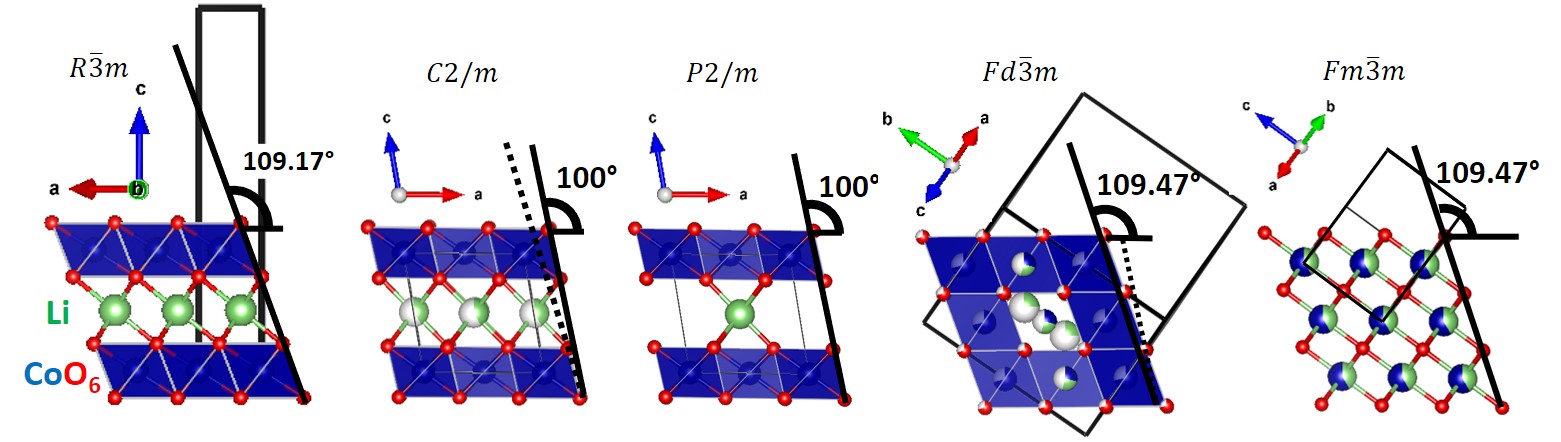
(a) Schematic crystal structures.

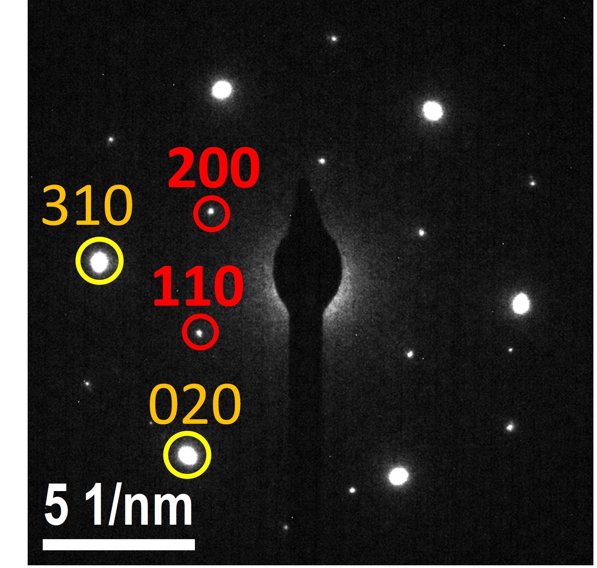
(b) 20^∘C $R\bar{3}m+C2/m$ $\langle 001\rangle$.

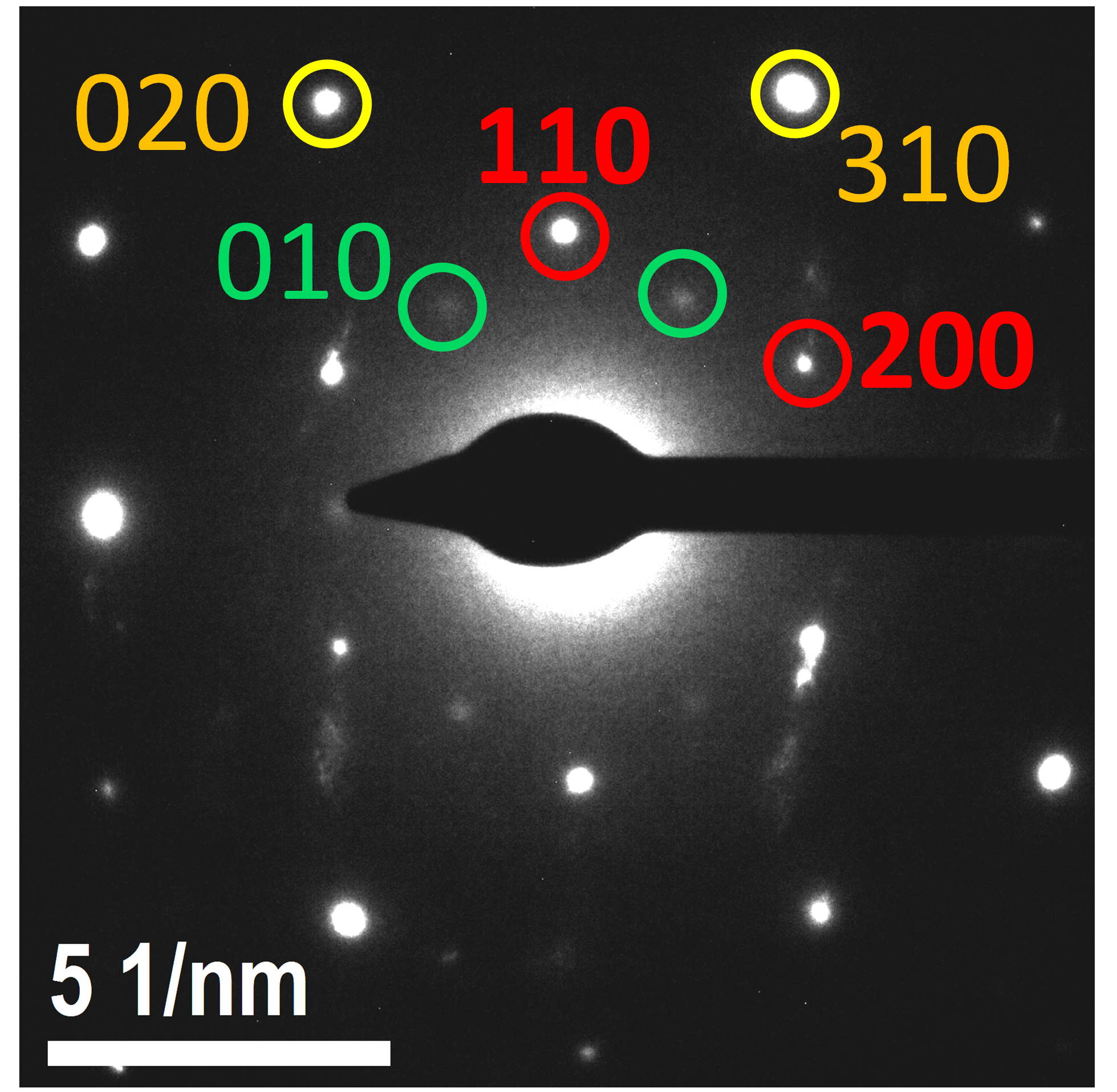
(c) 150^∘C $R\bar{3}m+C2/m$ $\langle 001\rangle$.

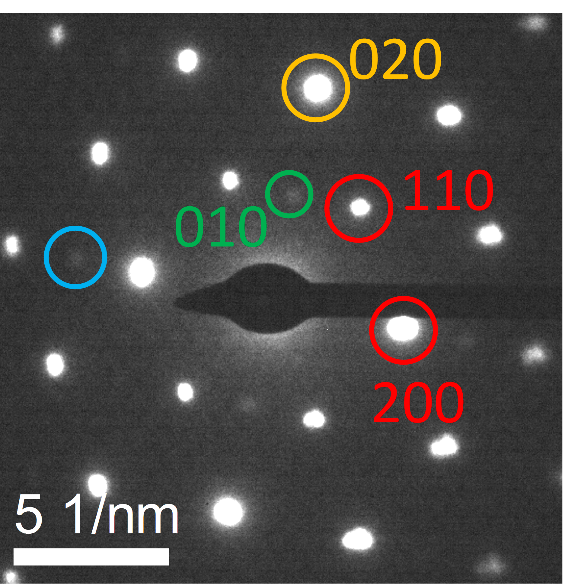
(d) 200^∘C
$R\bar{3}m$+$C2/m$+$P2/m$
$\langle 001\rangle$.

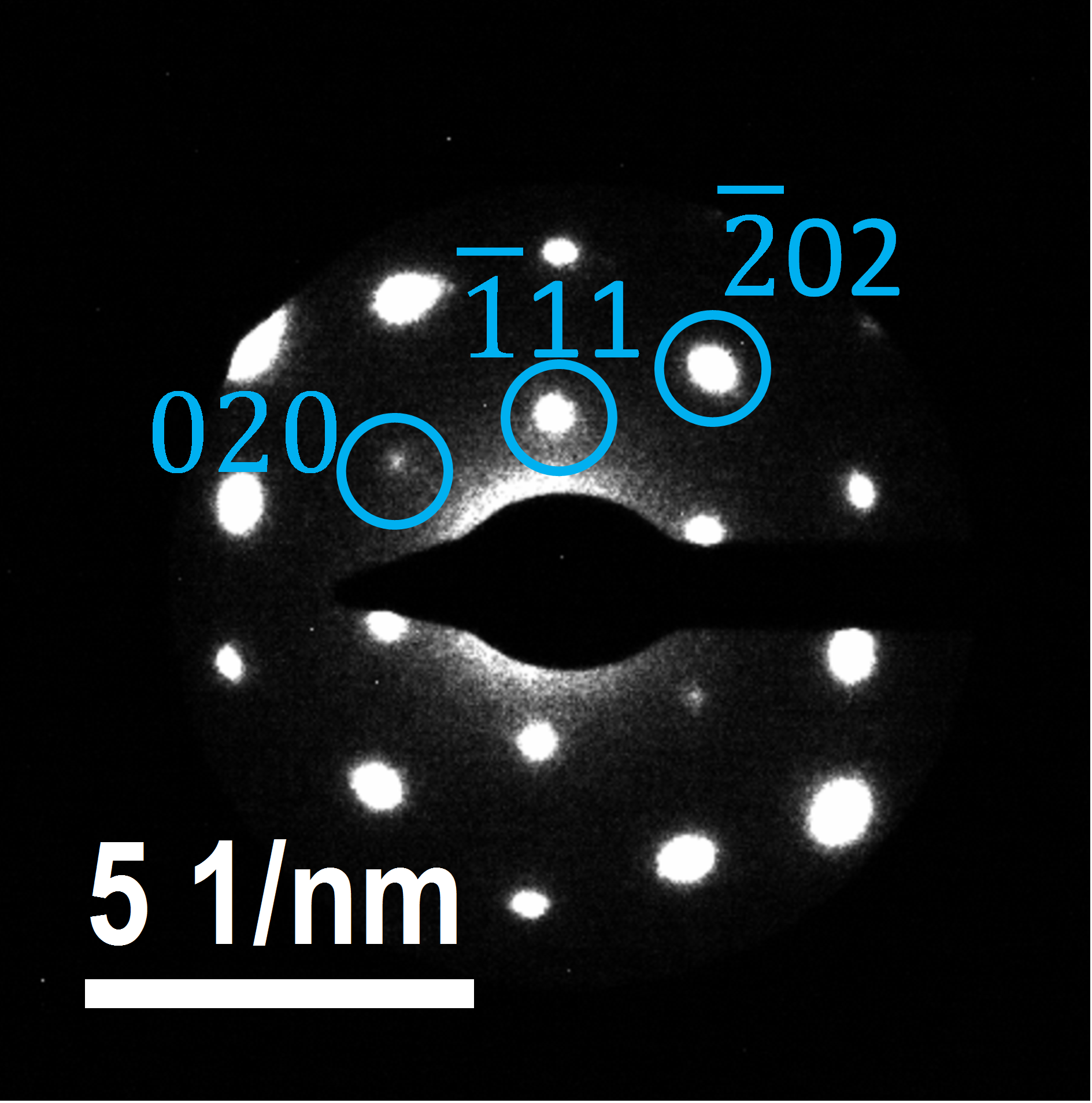
(e) 250^∘C
$Fd\bar{3}{m}$
$\langle 101\rangle$.

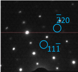
(f) 250^∘C
$Fd\bar{3}{m}$
$\langle 112\rangle$.

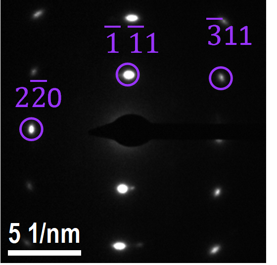
(g) 350^∘C
$Fm\bar{3}{m}$
$\langle 112\rangle$.

Fig. 1: Structure evolution upon annealing: (a) the schematic shows a repeatable part of structure which is preserved on phase transformations (not a unit cell). The pure CoO₆ atomic columns consist of blue octahedra. (b-g)SAED patterns for different annealing temperatures.

Fig. 1 illustrates the structure evolution of the Li_xCoO₂ nanoflakes with temperature, determined through the changes of TEM SAED patterns. The nanosheets typically were found lying with their octahedral sheets parallel to the carbon film. Before annealing, the diffraction pattern of a flake (Fig. 1(b)) showed two arrays of spots, an intense one circled in yellow that corresponds to a single crystal with $R\bar{3}m$ symmetry observed in the $[0001]$ zone axis, and a fainter array of spots circled in red, that corresponds to the formation of coherent nano-domains with the $C2/m$ symmetry. The latter is due to the slight distortion of the cell due to the loss of lithium (Fig. 1(a)) and the resulting repulsion between the CoO₂ layers. This structure corresponds to a random distribution of vacancies on the Li sites. It was shown before Motohashi et al. (2009); Chang et al. (2013) that the “O3”-type $C2/m$ phase (Fig. 1(a)) was stabilized for $x\approx 0.2-0.5$. A unique crystal orientation relationship with the $R\bar{3}m$ matrix was found, described as $[0001]\parallel[001]$, $(11\bar{2}0)\parallel(020)$. For more structural details, see Supplementary Table ST1.SM

After annealing at 150^∘C, the monoclinic $C2/m$ domains were coarsening reaching the size of the former $R\bar{3}m$ domains (Supplementary Fig. S2),SM as also evidenced in Fig. 1c through growing intensity of the corresponding reflections (in red). The prolonged TEM observation favored the appearance of additional 010 spots (in green), forbidden by the C lattice symmetry. These additional spots evidence the beginning of the phase transformation into the $P2/m$ phase on beam damage. In the $P2/m$ phase, 1:1 in-plane ordering of the Li-vacancy in Li_0.5CoO₂ takes placeKang et al. (2019) (Fig. 1(a)), as compared to the $C2/m$ phase. In Fig. 1(c), the three pairs of new reflections are attributed to three domain orientations Shao-Horn et al. (2003), which we also observed through energy filtered HRTEM (Supplementary Fig. S1(2)).SM For $T=200^{\circ}$C (Fig. 1(d)), the $C2/m$ and $P2/m$ phases coexist. The phase transformation of monoclinic phase into a cubic spinel-type $Fd\bar{3}m$ forming nano-domains was seen in HRTEM (Supplementary figs. S1(3,4).SM The orientation relationship (Figs. 1d-e) was found to be $[010]_{P}\parallel[101]_{F}$ and $[001]_{P}\parallel\approx[11\bar{1}]_{F}$.

The phase transformation to spinel was confirmed after annealing at $250^{\circ}$C (Fig. 1d-e, where the $Fd\bar{3}m$ phase was macroscopic (Fig. 1d-e and Supplementary Fig.S1).SM The transformation results from inter-layer diffusion of Co/Li, with octahedral and tetrahedral site occupancies. Combining our SAED with characteristic spot intensities (Fig. 1(e)), the EFTEM rod-like contrast (Supplementary Fig. S1(4)),SM and simulations of SAED/EFTEM of known spinel phasesWang et al. (2019); Gummow et al. (1993), we proposed the structure shown in Fig. 1(a), with 8a tetragonal sites partially occupied by Li and 16d (blue octahedra) and 16c sites alternating in the non-diagonal columns occupied by Co. The simulation of diffraction patterns were made in the $\langle 211\rangle$ zone axis, since it allowed a better discrimination of the spinel types by the relative intensities of their diffraction spots than in the $\langle 111\rangle$ zone axis (Supplementary Fig. S3a).SM The EFTEM contrast was simulated in $[101]$ zone axis (Supplementary Fig. S1(4-5)).SM We propose the suitable atomic site occupations, which are given in Supplementary table ST1.SM More studies are necessary to determine the precise site occupation. For $T=300^{\circ}$C, the flakes stayed in the $Fd\bar{3}m$ phase (Supplementary figs. S1-5 and S2-b).SM

For $T=350^{\circ}$C, some of the flakes transformed into the rocksalt $Fm\bar{3}m$ phase (Fig.1(a)) with about half lattice parameter (4.2 Å) and the same orientation of the $a$, $b$, $c$ lattice vectors. The transition is due to full mixing of Co and Li in 4a octahedral sites of $Fm\bar{3}m$ (fig. 1a) corresponding to the former 16c and 16d sites of the $Fd\bar{3}m$ structure. The partial phase transition is explained by different flake thicknesses, since it controls the rate of oxygen loss Sharifi-Asl et al. (2017). On top of newly formed $Fm\bar{3}m$, a remnant $Fd\bar{3}m$ phase was observed, which was similar to a fully disordered spinelWang et al. (2019). The energy filtered HRTEM (Supplementary fig.S1-6)SM showed the contrast, typical for spinel-like structure with the 8.3 Å lattice parameter, but with empty 8a sites (Supplementary fig. S3c).

IV.2 Overview of electronic transitions

Electronic structure changes induced by the structural modifications are studied in the following parts through EELS spectra of O-$K$ and Co-L edges. Fluctuations near the absorption edges are related to the probability of electron transitions from occupied to unoccupied electron levels. A schematic overview of the electronic transitions discussed here is given in Fig.2

The GGA band structure and DOS of LiCoO₂ in the $R\bar{3}m$ structure are shown in Fig. 3. Please note the different PDOS scale in the higher lying conduction band region. The top of the valence band is Co-$d$-$t_{2g}$ like, while deeper bands have more O-$2p$ character. The lowest conduction band is dominated by Co-$3d$ while the higher bands in the range 6-10 eV have mainly Li-$2s2p$ and O-antibonding contributions. There is also a Co-$4s$ contribution which however is stronger between 12-14 eV. The bands in this energy range have strong dispersion and are essentially free-electron like. In the GGA, the band gap is somewhat underestimated and amounts to 0.89 eV for the indirect gap.

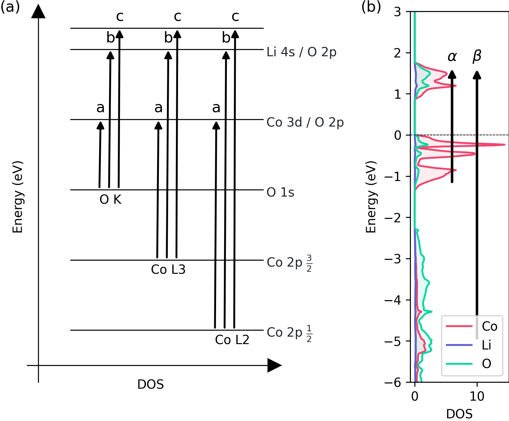
Fig. 2: Schematic of energy transitions.

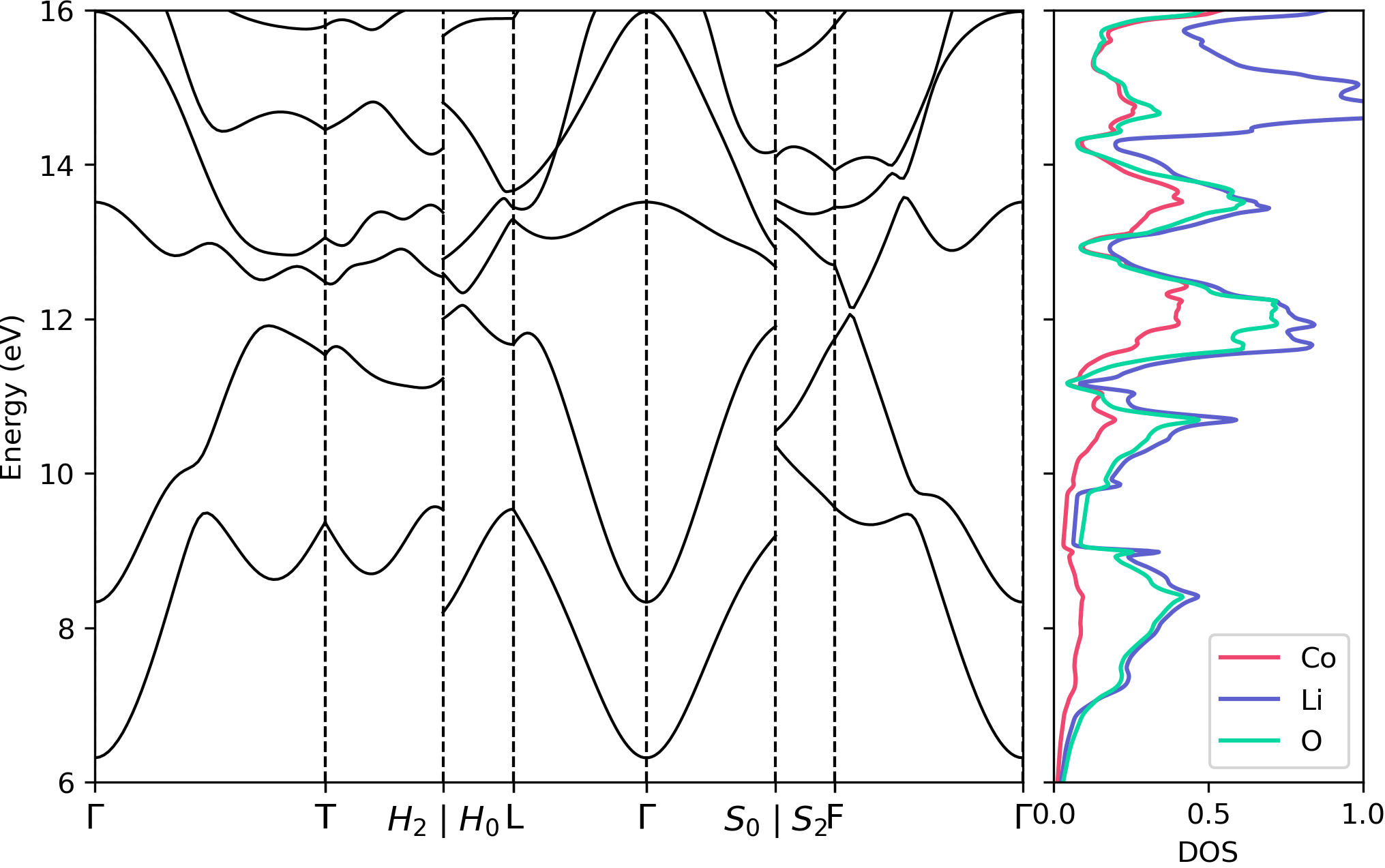
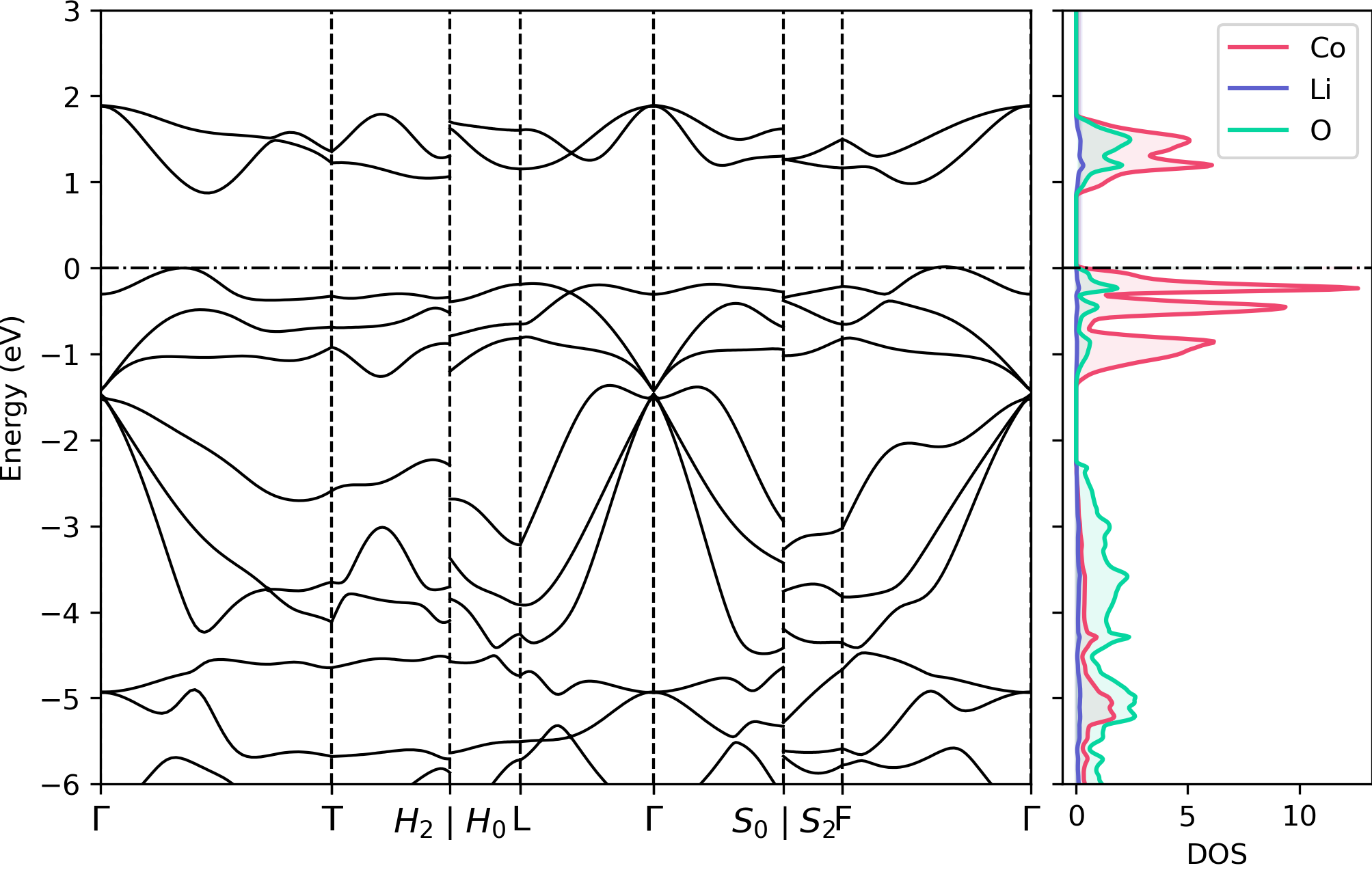
Fig. 3: GGA band structure and PDOS of LiCoO₂ in $R\bar{3}m$ structure in two energy intervals.

IV.3 O-$K$ edge spectra

In Fig. 4, the inset shows the typical EELS O-$K$ edge spectrum for 20^∘C (non-annealed) sample (spectra recorded at all studied temperatures on several particles and processed to build this figure are given in Supplementary fig. S4).SM The pre-peak “a” (Fig. 2) comes from electron transitions from the O-$1s$ core level towards the lowest conduction band,Kikkawa et al. (2014) which is the Co-$3d$-$e_{g}$ band, where $e_{g}$ refers to the irreducible representation in the octahedral group of the Co octahedral environment. These are antibonding hybridized Co-$3d$ - O-$2p$ states. The components “b” and “c” are due to transitions towards higher conduction bands, which involve both the Li-$2s$ and Co-$4s$ derived bands antibondng with O-$2p$ and are essentially free-electron like bands.

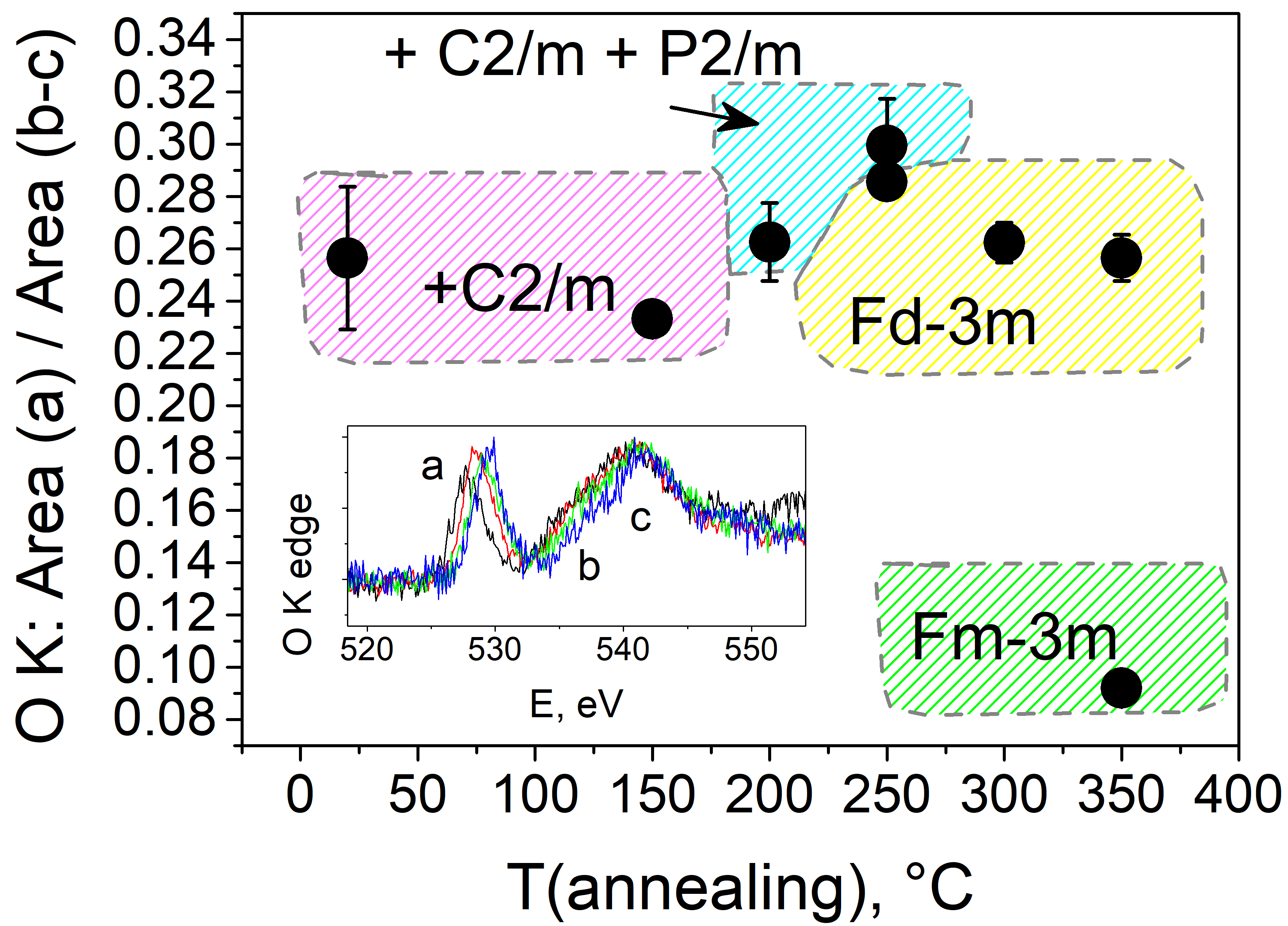
Fig. 4: EELS study of O K edge: (a) the ratio of integrated area $A(a)/A(b,c)$ of the pre-peak “a” versus main peak components “b” and “c”, as identified in the inset, which shows the spectrum of Li_0.37CoO₂ at 20^∘ C.

According to Zhao et al. Zhao et al. (2010) the relative intensity of the pre-peak “a” to the “b/c” peaks is connected to the degree of Co $3d$ - O $2p$ hybridization. We thus studied this ratio of peak intensities as function of annealing temperature, $T$, as shown in Fig.4. For annealed nanoflakes, in the range $T=20^{\circ}$C - 200^∘C, the ratio first increased, which would indicate an increase of the Co-$3d$ – O-$2p$ hybridization for the $R\bar{3}m\rightarrow C2/m\rightarrow P2/m$ phase sequence. On the other hand, for $T=200^{\circ}$C to $350^{\circ}$C and the transition $Fd\bar{3}m\rightarrow Fm\bar{3}m$, the $A(a)/A(bc)$ ratio decreased dramatically.

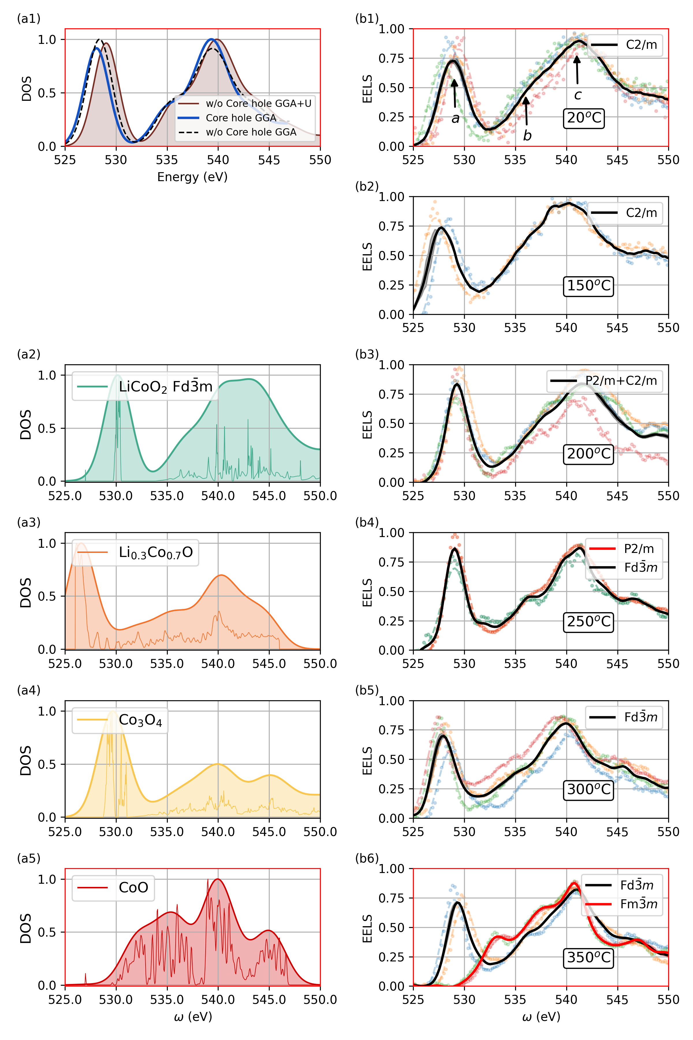
Fig. 5: (a) Simulated O-$K$ spectra for various systems: (a1) comparison of Eq.(1) including O-$1s$ core hole and matrix elements explicitly with simple O-$p$ PDOS both in GGA and with O-$p$ PDOS in GGA+U ($U=5$ eV) for LiCoO₂ in $R\bar{3}m$ structure, (a2-a5) O-$p$ PDOS in GGA+U for: (a2) LiCoO₂ in $Fd\bar{3}m$ model, (a3) Li_0.3Co_0.7O in $Fm\bar{3}m$ structure, (a4) Co₃O₄ in spinel $Fd\bar{3}m$ structure and (a5) CoO in rocksalt $Fm\bar{3}m$ structure. (b) Experimental EELS for different samples (shown in scatter plots), with average data smoothened using Savitzky-Golay filterSavitzky and Golay (1964) shown in red/black for various temperatures

Alternatively, we compare these spectra directly with calculated O-$K$ spectra for various model systems in Fig. 5. First, in (a1) we compare different computational approaches for LiCoO₂ in the $R\bar{3}m$ structure. This shows that the calculation taking the core-hole and O-$1s$ to band states matrix elements explicitly into account according to Eq. 1 is almost indistinguishable from the simple O-$2p$ PDOS. Adding $U$ to the GGA just shifts the Co-$d$ bands up slightly but the spectra in either of these models agree well with the experimental spectrum in (b1). The zero of energy in our calculation is the highest occupied band (VBM) but was then shifted by 527 eV to align the first “a” peak with experiment. A Gaussian broadening by $\sim$1 eV is applied to our calculated spectrum after removing the filled part of the PDOS. The unbroadened spectrum is shown in thinner lines underneath the shading. We expect negligible changes in the closely related $C2/m$ and $P2/m$ phase. In the experimental panels (b1-b6) the black thicker line is a smoothed average over different samples. The sample details are provided in Supplemental Information Fig. S4(a).SM

Next, in panels (a2-a4) we show GGA+U results for the O-$p$ PDOS for various models in an attempt to qualitatively understand changes in these spectra. For the $Fd\bar{3}m$ calculations, we used a model provided by Materials ProjectMP with the above spacegroup. It contains both Li and Co exclusively in octahedral sites. One can see that there is little qualitative change between the $R\bar{3}m$ and $Fd\bar{3}m$ spectra, just as there is little change between the $P2/m$ and $Fd\bar{3}m$ spectrum in panel (b4). We also calculated a $Fm\bar{3}m$ spectrum using a supercell of the rocksalt structure with a random occupation of Li and Co atoms in a ratio of $3/7$ Li/Co. Finally, we also considered spinel Co₃O₄ and rocksalt CoO without any Li.

We note that in the rocksalt phase in GGA the $t_{2g}$ to $e_{g}$ crystal field splitting in the octahedral environment is reduced compared to that in $R\bar{3}m$ because of the larger Co-O distance. On the other hand, the bands have significantly larger band dispersions, related to the more 3D network type arrangement of Co and Li compared to the layered structure in $R\bar{3}m$. Because of this we no longer have a gap between separated $t_{2g}$ and $e_{g}$ bands but these two overlap and lead to a metallic band structure, in disagreement with experiment. This is why we need to use GGA+U to obtain a qualitatively meaningful electronic structure. The gap in such systems arises from the formation of magnetic moments and correlation effects in the partially filled Co-$3d$ derived bands. For Co₃O₄ we obtain a ferromagnetic band structure in the primitive cell when using GGA+U. For CoO we use an SQS model with random distribution of up and down spins to model the paramagnetic state. Likewise for the Li containing $Fm\bar{3}m$ structure we use the SQS approach to model both the Li/Co random location and up and down spins on Co sites. Band structures for these cases are shown in Supplemental Information Figs. S7-S9.SM Even with GGA+U, for the Li_0.3Co_0.7O $Fm\bar{3}m$ structure we obtain a metallic band structure with the Fermi level close to the top of the $d$ $t_{2g}$ band (Fig. S9).

We can see that qualitatively all the simulated O-$K$ spectra stay rather similar with similar “a” and “b/c” peak relative positions and intensity ratio. The exception is CoO where the a peak is signficantly less intense and closer to the b/c peaks and this agrees with the experimental observation for the $Fm\bar{3}m$ spectra. From the entire series of experimental data, taking in to account the sample to sample variation, the most obvious change occurs for the $Fm\bar{3}m$ phase at 350^∘C. From Fig. S4(a) and Fig.5(b6), one can see that the strong drop in $A(a)/A(bc)$ is related to a shift in the “a” peak to higher energies in qualitative agreement with the CoO result in Fig.5(a5). This can also be seen in the simulations by Zhao et al. Zhao et al. (2010), with which our calculations agree quite well, even though their calculation did not include the core-hole induced changes in the density of states and was purely GGA. The experimental spectra for the $Fm\bar{3}m$ phase are much more resemblant of the pure CoO phase than of the $Fm\bar{3}m$ Li_0.3Co_0.7O model we calculated. This is an indication that at these higher temperatures, the system may have lost some Li from the rocksalt phase parts of the sample by diffusion into other regions.

IV.4 Co-$L_{2,3}$ edge spectra

The origin of the Co $L_{3}$,$L_{2}$ edge components is explained schematically in Fig. 2. They correpond to transitions from core levels Co $2p_{3/2}$ ($L_{3}$) and Co $2p_{1/2}$ ($L_{2}$). Both $L_{3}$ and $L_{2}$ include three components each, marked as “a-c” and “d-f”. Importantly, the intensity ratio $A(L_{3})/A(L_{2})$ in $3d$ transition metals is recognized as a parameter which reflects the cation valenceZhao et al. (2010); Wang et al. (2000); Egerton (2011). This is related to many body effects in these open shell states. Fig. 6 presents the variation of Co valence, deduced from the calibration curve for $A(L_{3})/A(L_{2})$, presented in Supplementary Fig. S5.SM The step-like changes of the Co valence in Fig.6 are connected with the phase changes. Prior to annealing the mean Co valence of Li_0.37CoO₂ was around 3.3. A charge compensation of the Li loss handled by Co only would give a valence of 3.63. The lower experimental valence, together with the Co $3d$- O-$2p$ hybridization revealed by the O-$K$ pre-peak, indicates a contribution from O-$2p$ holes in the charge compensation. This is also consistent with findings by Wolverton and ZungerWolverton and Zunger (1998) that within a sphere around Co, little change in charge density is found upon Li loss but rather a change in Co-O bonding. At 150^∘C, the Co valence is lowered to 3.15, probably due to the increase of covalency and Co-O hybridizations in the growing $C2/m$ phase. The gradual growth of $P2/m$ domains induces an increase of the mean Co valence. The $1:1$ ordering of the Li vacancies drives the charge ordering on Co sites, inducing Co atoms which donate to O more electronic charge than in a random vacancy distribution.Miyoshi et al. (2018); Kang et al. (2019) Essentially, Co⁴⁺ is formed near the Li vacancies. This is, probably, the reason why the Co valence is larger in $P2/m$ phase than in $C2/m$, although still with a degree of covalency in the Co-O bond. Finally, for $T>250^{\circ}$C, $Fd\bar{3}m$ and $Fm\bar{3}m$ phases have reduced average Co valence $<3+$, which evidences the increasing presence of reduced cations Co²⁺. The pure monoxide CoO has also the $Fm\bar{3}m$ rocksalt structure.Redman and Steward (1962) The reduction in average valence by the presence of Co²⁺ in the rocskalt phase is consistent with a loss of Li from these regions found in the previous section from the O-$K$ spectra.

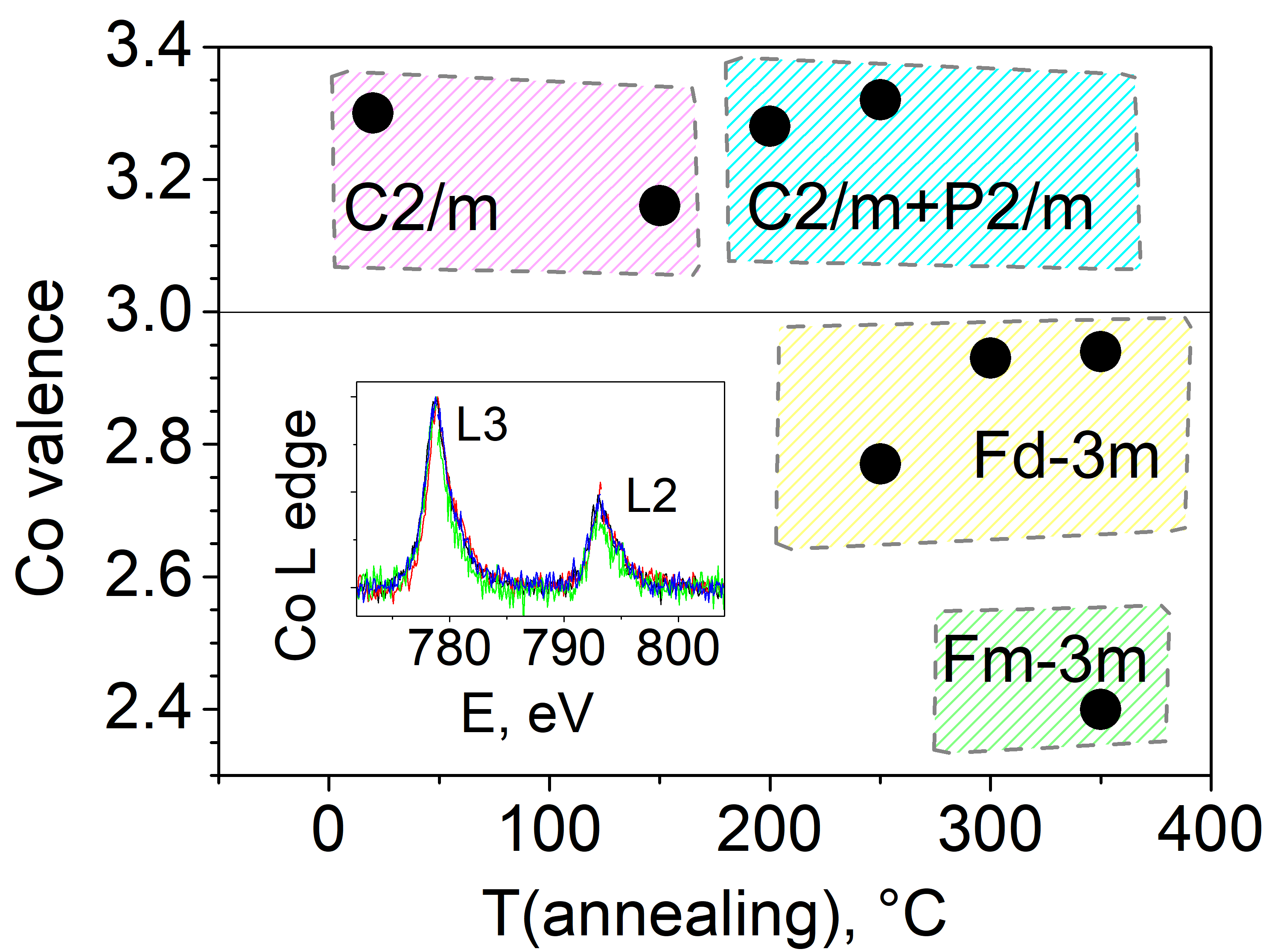
Fig. 6: Average Co valence as deduced from the L₃/L₂2 edge peak ratio.

IV.5 Low energy EELS

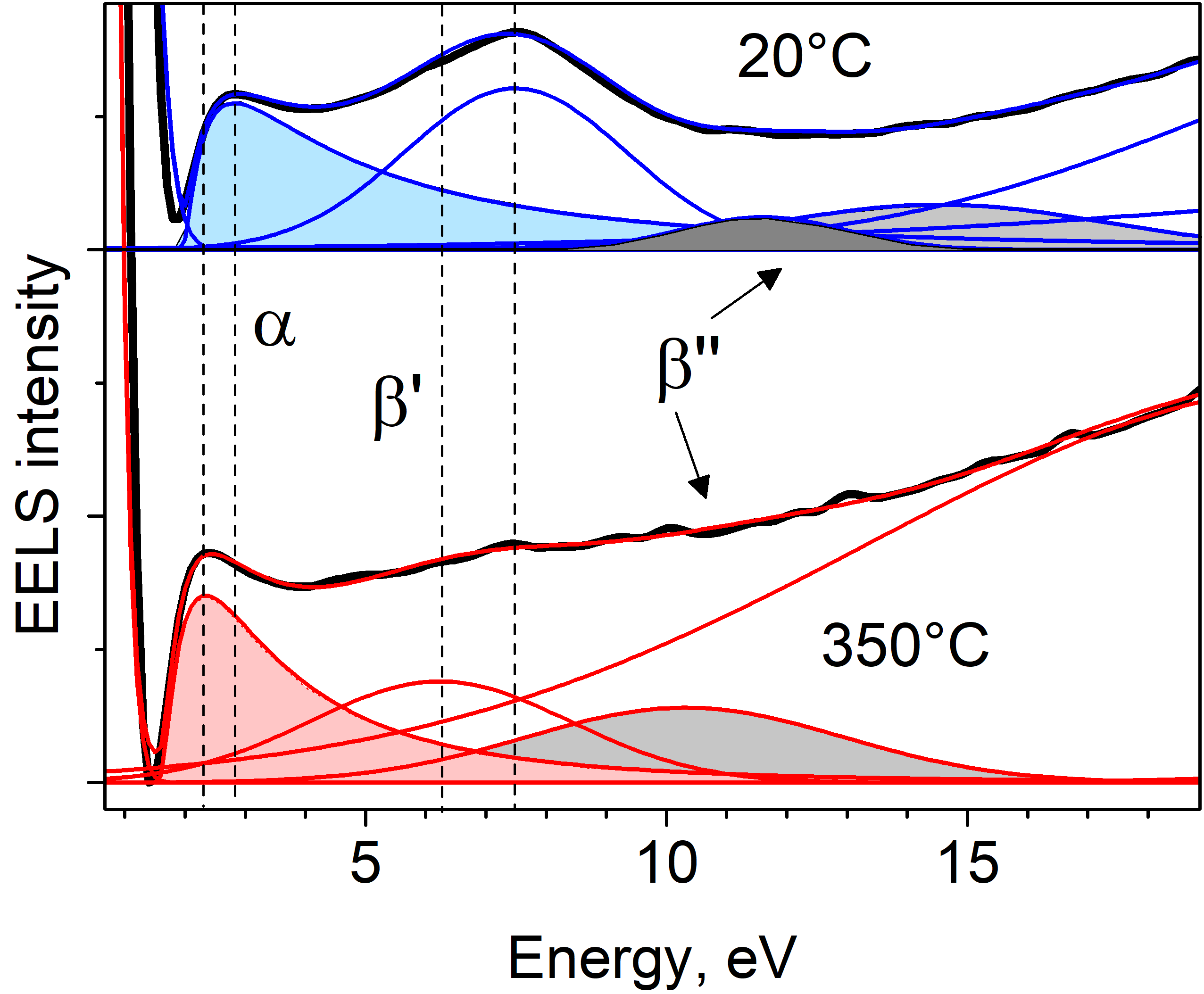
(a)

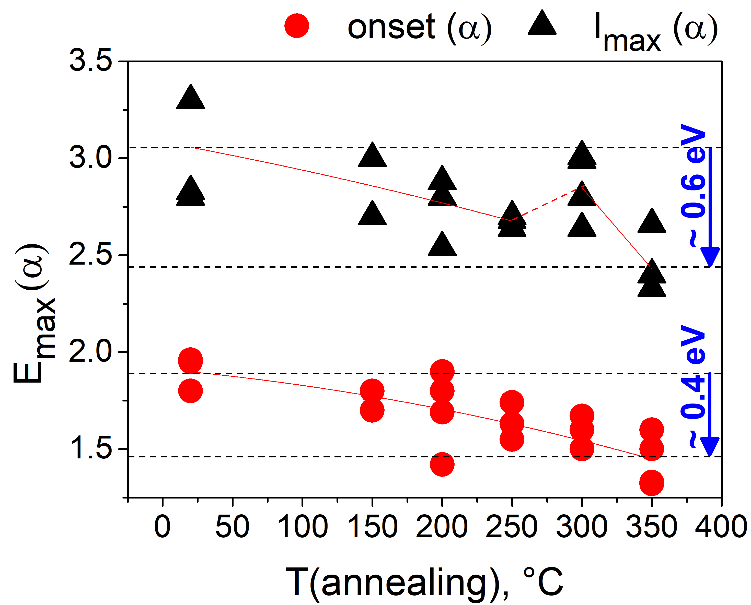
(b)

Fig. 7: Low energy loss spectra for near-bandgap electronic structure: (a) the fit model shown for two spectra after annealing at 20^∘C and 350^∘C, (b) onset of transition $\alpha$ and it’s maximum plotted for all nanoflakes.

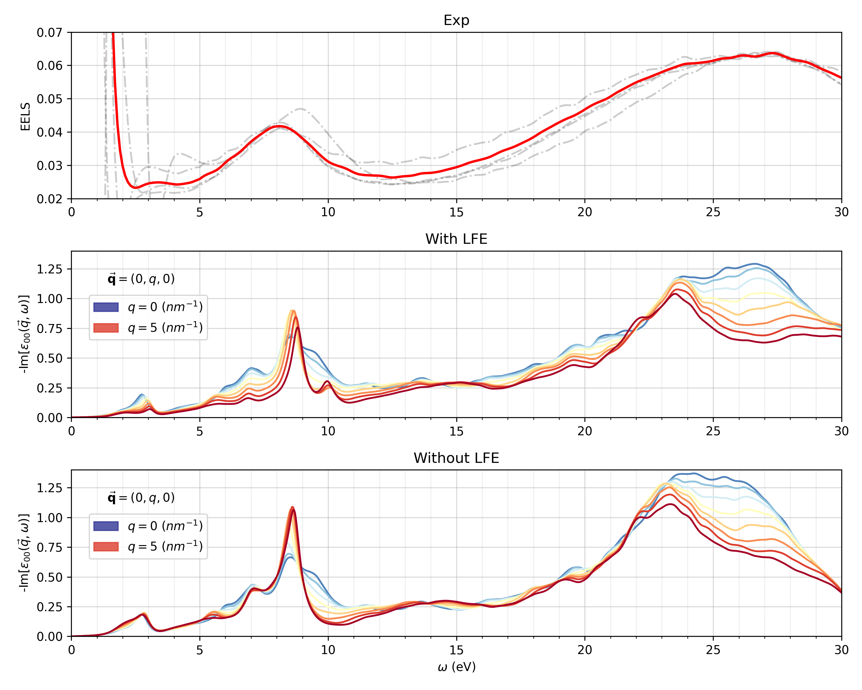
Fig. 8: EELS, from to to bottom: (a) experimental data at 20^∘C the red curve is an average over three samples; Calculated $\mathcal{A}_{\operatorname{ELSS}}(\mathbf{q},\omega)$ at $\mathbf{q}=(0,q,0)$ for $q=0$(blue) to $q=0.5$(red) with (b) and without(c) Local Field effects.

.

Fig. 7 shows the measured low energy EELS for two temperatures. The spectrum is deconvolved into an asymmetric $\alpha$ peak at about 3 eV and rather broad $\beta$ peak at about 7.5 eV and a weak higher feature labeled $\beta^{\prime\prime}$. As indicated in Fig. 2 one may loosely associate the $\alpha$ peak to transitions from the topmost Co-$t_{2g}$ part of the valence band to the $e_{g}$ conduction bands and the $\beta$ peak to transitions from, a peak in density of states deeper in the valence band with more O-$2p$ character to the same conduction band. In between there is a region of low density of valence band states which explains qualitatively why the $\alpha$-peak has a low density tail toward higher energies and asymmetric shape. As shown in Supplementary Information (Fig. S10),SM a simple convolution of the occupied and empty densities of states, ignoring any momentum conservation provides this type of general shape with an asymmetric $\alpha$ and a broad $\beta$ peak.

However, a better approach is to compare these EELS spectra with the calculated loss spectrum, which is shown in Fig. 8. As mentioned in the computational methods section, this corresponds to the $q\approx 0$ energy longitudinal response function. To be clear this corresponds to vertical transitions but integrated over the whole Brillouin zone. We here show calculations as function ${\bf q}$ and both including and neglecting local field effects. The first weak peak around 2.5 eV agrees well with the experimental $\alpha$-peak. The next strong peak centered at $\sim$8 eV agrees well with the experimental $\beta$-peak. Even finer structure be recognized in the experiment as shoulder structures. The broad strong peak between 20-30 eV corresponds to the plasmon. Using, $\omega_{P}=\sqrt{4\pi ne^{2}/m_{e}}$ including 18 valence electrons, so not including the O-$2s$ electrons as valence, one obtains a plasmon energy of 27 eV, while including the O-$2s$ would give 30 eV. On the other hand the O-$2s$ derived bands lie about 20 eV below the VBM, so band-to-band transitions from these to the $e_{g}$ conduction band are also expected in this energy range, overlapping with the dominant plasmon peak.

In this figure we show the spectrum as function q up to about 5 nm^-1. One may see that including local field effects, the $\alpha$ peak gradually becomes smaller as q increases but this effect is not seen when local field effects are neglected. In the present experiment, we estimate that we integrate the spectrum near ${\bf q}=0$ up to about $q=5$ nm^-1. To measure the spectrum as function of ${\bf q}$ one would need to vary the central ${\bf q}$ away from the (000) spot in small steps and within an even smaller range or spot size $\delta q$. Such measurements were done for the Li-$1s$ loss spectrum in Ref. Kikkawa et al., 2018.

Fig. 7 shows that both the onset and the location of the maximum intensity of the $\alpha$-peak shift to the lower energy on increase of the annealing temperature. Within the error of measurements, we observe a decrease of these values by $\sim$0.4 and $\sim$0.6 eV respectively. This decrease indicates a decrease of the $t_{2g}$-$e_{g}$ gap and it agrees with the predictionTarascon et al. (2004); Miedzinska et al. (1987) of a band gap decrease with Co valence decrease. The decrease in valence is also correlated with changes in Co-$3d$ - O-$2p$ hybridization or degree of covalency as indicated by the O-$K$ spectra.

On the other hand, in CoO and Co₃O₄ the correlated electronic structure can no longer be explained purely within a standard DFT band-structure picture,van Elp et al. (1991) although it is still possible to obtain a gap within DFT+U even for the disordered paramagnetic phase using a polymorphous description, which includes local symmetry breaking and spatial fluctuations.Trimarchi et al. (2018) Trimarchi et al. Trimarchi et al. (2018) obtain a gap of 2.25 eV for CoO in the paramagnetic rocksalt structure. Our own calculations of the band structure within GGA+U (given in the Supplemental Information S8)SM give a gap of 1.94 in paramagnetic CoO and this is indeed somewhat smaller than the gap obtained for LiCoO₂ in either the $R\bar{3}m$ (2.746 eV) or $Fd\bar{3}m$ phases (2.710 eV).

From previous literature, the prediction of decreasing gaps Tarascon et al. (2004); Miedzinska et al. (1987) is found to hold for Li_xCoO₂ with varying $x$. In the extreme case of $x=0$, pure Co₃O₄ in the $Fd\bar{3}m$ phase also has been reported to have a smaller band gap (1.6 eV),Smart et al. (2019), which, however, is related to a small polaron formation. Note that this value of the gap is smaller than ours (1.724 eV) which does not include such polaronic effects. Whether or not such polaronic effects are observed may depend on the time scale of the method with which the gap is probed because the polaron formation occurs at the time scale of the atomic displacements. For example, one typically observes a polaron in photoluminescence but not in optical absorption. The present EELS measurements are closer to optical absorption.

In the present case of Li_0.37CoO₂ this reduction of the gap appears to be caused by the structural transitions, and changes of cation order. It is well known that disorder may reduce the band gap by forming defect like band tails in the gap near the band edges. However, in the present case, the situation may be more complex by the increasing importance of not only structural and cation disorder fluctuations but also magnetic moment formation and fluctuations in magnetic moment orientation and $d$-band correlation effects, including possibly strong electron-phonon coupling as occurs in self-trapped polaron formation. Disentangling these various effects is beyond the scope of the present paper.

IV.6 Conductivity

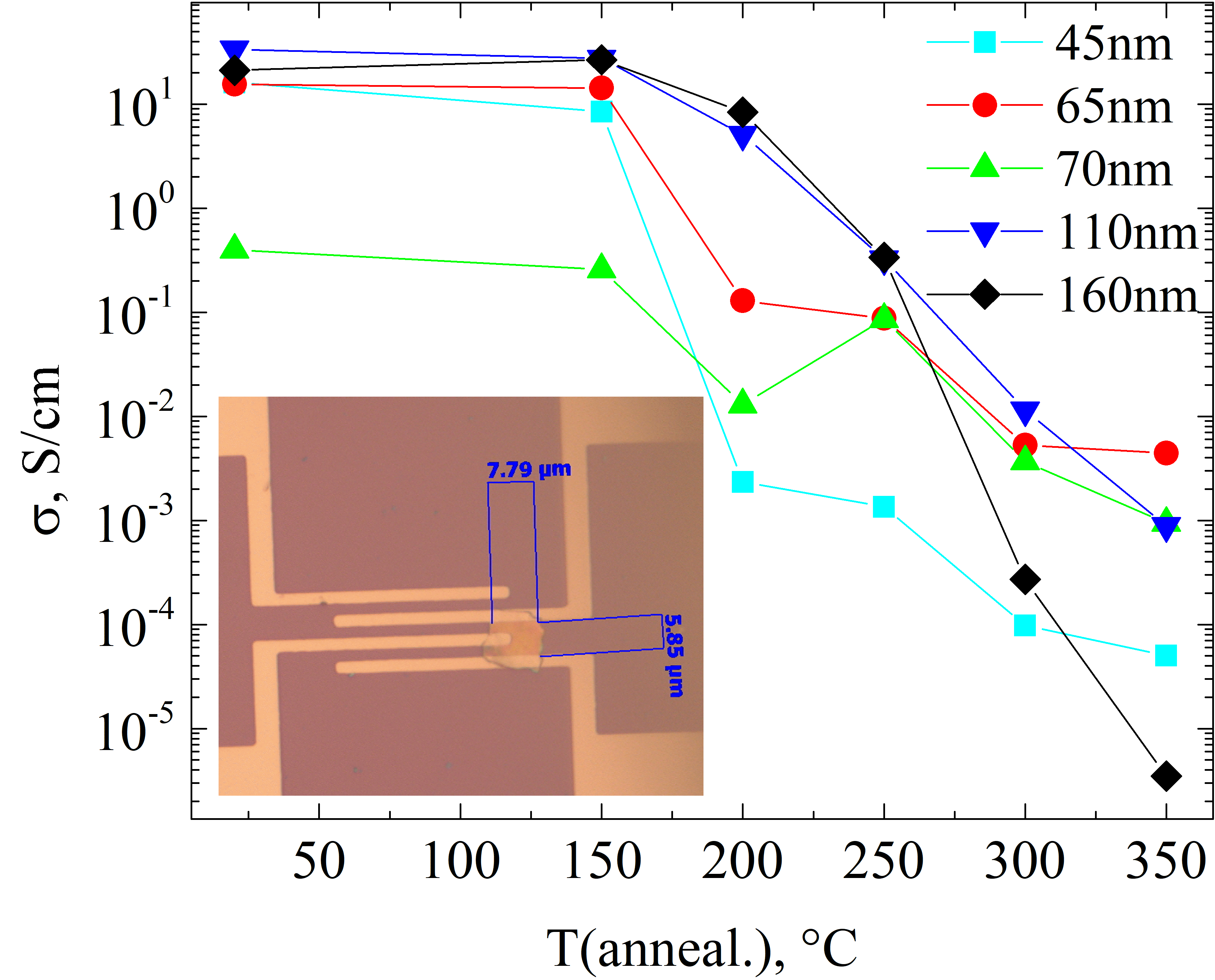
Fig. 9: Electrical conductivity as function of annealing temperature. Inset: device structure showing electrical contacts.

Finally, we examine how the conductivity changes with annealing temperature and whether it is related to the observed band gap decrease and changes in valence, hybridization evidenced by the spectroscopic investigations of the previous sections. The conductivity changes as function of annealing temperature are shown in Fig. 9. The conductivity remains at its highest value for $T\leq 150^{\circ}$C corresponding to the $C2/m$ phase. A decrease in conductivity is observed for $T\geq 150^{\circ}$C. At 200^∘C it corresponds to a macroscopic $P2/m$ matrix, possibly with the beginning of $Fd\bar{3}m$ nanodomains at 200^∘C (Supplementary Fig. S1(3)).SM This $Fd\bar{3}m$ phase with its lower covalency and O-$2p$ – Co-$3d$ hybridization at the conduction band edges is, probably, at the origin of the start of conductivity decrease, as charge carriers tend to become more localized for less hybridized levels. This decrease is stronger for the macroscopic $Fd\bar{3}m$ and $Fm\bar{3}m$ phases at 250-350^∘C. The spinel structure for $x=2/3$ was reported as insulating in STM when cation migration forces random occupation of sites.Miyoshi et al. (2018), In our case, the spinel type phase with $x\approx 1/3$ is also found to be insulating.

On the other hand, as mentioned earlier, there are also indications that on heating the Li concentration may be decreasing in the sample due to out-diffusion. The poorer the system is in Li, the more correlated the electronic structure becomes with increasing polaronic effectsSmart et al. (2019) and this may also be part of the reason for the conductivity decrease. While for Li_xCoO₂ in the $R\bar{3}m$ and the closely related $C2/m$ and $P2/m$ structures, a normal band picture still holds with some $p$-type hole doping due to $x<1$, in the $Fd\bar{3}m$ and even more so, in the $Fm\bar{3}m$ phases, the starting picture of a band insulator becomes untenable because of the overlapping of the $t_{2g}$ and $e_{g}$ bands. In the $Fd\bar{3}m$ one would even have inverted $t_{2g}$ and $e_{g}$ levels at tetrahedral Co-sites. The origin of the band gap in this case does no longer arise from a well separated nearly filled $t_{2g}$ band below an empty $e_{g}$ band with low-spin configuration, but from correlation effects leading to magnetic moments and a gap forming between majority and minority spin electrons. The nature of the conductivity is thus clearly expected to be dramatically changing once these phases come into play. The inter-layer cation mixing might thus be considered to be detrimental for the conductivity.

V Conclusions

To conclude, we have presented in this paper a comprehensive study of the structural changes, electronic properties as derived from electron energy loss spectroscopy correlated with first-principles calculations, and conductivity measurements of Li_0.37CoO₂ nanoflakes subjected to heating. The O-$K$ spectra were interpreted in terms of O-$p$ PDOS modulated by the dipole matrix elements linking the conduction states to the O-$1s$ core-wavefunction in an all-electron approach and taking the presence of the core-hole into account. The low energy loss spectra were well described by the calculated loss function $-\mathrm{Im}[\varepsilon^{-1}({\bf q},\omega)]$ for small q. Predictions are made for the ${\bf q}$-dependence of these spectra. They offer a basic interpretation of the main features, whose trends are studied upon heating.

The Li_0.37CoO₂ flakes are initially (between 150^∘ C and 200^∘ C annealing temperature) found to experience phase transitions from the rhombohedral $R\bar{3}m$ phase to the monoclinic phases $C2/m$ and $P2/m$ with disordered and ordered, Li vacancies respectively. During these transitions, the Co valence increases in parallel with increasing Co-$3d$ – O-$2p$ hybridization as evidenced from the interpretation of the peak ratio changes in O-$K$ and Co-$L_{2,3}$ spectra. Upon further heating above 250^∘C and completed by 350^∘C when partial or full Li-Co interlayer mixing happens in the spinel-type $Fd\bar{3}m$ and rocksalt-type $Fm\bar{3}m$ phases, the Co nominal valency decreases, as well as the hybridization of Co-$3d$ – O-$2p$ states. A band gap decrease is observed when these phases start to form. The increasing presence of Co²⁺ indicated by $L_{2,3}$ spectra is consistent with a loss of Li from the rocksalt phase regions, as also indicated by the O-$K$ spectra. These changes are related to the dramatically modified band structure which is no longer in a low-spin state. Band structure calculations at the GGA level indicate a significant overlap of $t_{2g}$ and $e_{g}$ bands in the $Fm\bar{3}m$ phase with a metallic band structure, which becomes unstable toward magnetic moment formation. The latter can be described within the DFT+U methodology and allowing the magnetic moments to occur in a disordered manner. This leads to a three to six orders of magnitude decrease in conductivity at temperatures where these phases start to form because of increased Li and Co interdiffusion forming a 3D network instead of a layered phase.