On Distributionally Robust Multistage Convex Optimization: New Algorithms and Complexity Analysis
Abstract
This paper presents an algorithmic study and complexity analysis for solving distributionally robust multistage convex optimization (DR-MCO). We generalize the usual consecutive dual dynamic programming (DDP) algorithm to DR-MCO and propose a new nonconsecutive DDP algorithm that explores the stages in an adaptive fashion. We introduce dual bounds in the DDP recursions to prevent the growth of Lipschitz constants of the dual approximations caused by recursive cutting plane methods. We then provide a thorough subproblem-oracle-based complexity analysis of the proposed algorithms, proving both upper complexity bounds and a matching lower bound.
To the best of our knowledge, this is the first nonasymptotic complexity result for DDP-type algorithms on DR-MCO, which reveals that in some practical settings the new nonconsecutive DDP algorithm scales linearly with respect to the number of stages.
Numerical examples are given to show the effectiveness of the proposed nonconsecutive DDP algorithm and the dual-bounding technique, including the reduction of the computation time or the number of subproblem oracle evaluations, and the capability to solve problems without relatively complete recourse.
Keywords:
distributionally robust convex optimization,
multistage optimization,
dual dynamic programming algorithm,
complexity analysis,
cutting plane method
1 Introduction
Distributionally robust multistage convex optimization (DR-MCO) is a sequential decision making problem with convex objective functions and constraints, where the exact probability distribution of the uncertain parameters is unknown and decisions need to be made considering a family of distributions. DR-MCO provides a unified framework for studying decision-making under uncertainty. It includes as special cases both multistage stochastic convex optimization (MSCO), where some distribution of the uncertain parameters is known and the expected cost is to be minimized, and multistage robust convex optimization (MRCO), where the uncertainty is described by a set and the worst-case cost is to be minimized. DR-MCO as a general decision framework finds ubiquitous applications in energy system planning, supply chain and inventory control, portfolio optimization, finance, and many other areas (see e.g. [39, 6]).
DR-MCO is in general challenging to solve, due to the fast growth of the number of decisions with respect to the number of decision stages [36, 15, 17]. Meanwhile, real-world problems are often endowed with special structures in the uncertainty. In particular, the uncertainty may exhibit stagewise independence (SI), i.e., the uncertainty in different stages are independent from each other. Many uncertainty structures, such as autoregressive stochastic models, can be reformulated to satisfy SI [41]. This versatile modeling capability of SI has great implications on computation. It allows recursive formulations of cost-to-go functions in each stage of a DR-MCO to be independent of the outcomes in its previous stages, thus making efficient approximations of the cost-to-go functions possible. Indeed, SI has been successfully exploited by various algorithms in solving MSCO and MRCO [37, 32, 17, 30, 3, 4, 1, 43, 38].
Among algorithms for DR-MCO, dual dynamic programming (DDP) is a prevalent class of recursive cutting plane algorithms that originate from nested Benders decomposition for multistage stochastic linear optimization [8, 28]. The earliest form of DDP for MSCO using stochastic sampling method was proposed in [29], known as stochastic dual dynamic programming (SDDP), where in each iteration the scenarios are sampled randomly and solved sequentially before updating the cost-to-go functions recursively. The algorithm has since been widely adopted in areas such as energy systems scheduling [16, 11, 40]. The deterministic sampling version of DDP was later proposed, which uses both over- and under-approximations for sampling and termination [3, 4]. DDP has also been extended to multistage stochastic nonconvex problems [43, 44, 1, 42]. Robust dual dynamic programming (RDDP) is proposed for multistage robust linear optimization [17]. Due to its intrinsic difficulty, the uncertainty sets are assumed to be polytopes such that the subproblem in each stage can be solved via a vertex enumeration technique over the uncertainty set. Similar to the deterministic DDP, RDDP constructs both over- and under-approximations to select the worst-case outcome. Moreover, it has the advantage of being able to terminate the algorithm with a guaranteed optimal first stage solution, in contrast to the commonly used decision rules [24, 7, 21]. Recently, DDP has been further extended to DR-MCO with promising out-of-sample performance [2, 22, 31, 14]. In particular, [31] uses an ambiguity set defined by a -distance neighborhood. In [14], the ambiguity sets are taken to be Wasserstein metric balls with finite support and centered at the empirical distributions, and the algorithm is shown to converge asymptotically with stochastic sampling methods. We comment that all of the above variants of DDP algorithms rely on the assumption of relatively complete recourse (RCR), while it is indeed possible to have MSCO that do not satisfy such an assumption [27].
The convergence analysis of DDP begins with multistage linear optimization [32, 37, 26, 10], where an almost sure finite convergence is established based on polyhedral structures. In [18], an asymptotic convergence is proved for MSCO problems. Due to the multistage structure, a main complexity question concerning DDP is the dependence of its iteration complexity on the number of decision stages, which is recently answered for MSCO, independently in [25, 42]. In particular, [18, 25] assume RCR and, moreover, the value functions are all Lipschitz continuous. A weaker regularity assumption concerning exact penalization is made instead in [42] that allows the DDP algorithm to work without RCR. However, it is not yet known whether the DDP algorithm, together with the complexity analysis, works for DR-MCO. The present paper introduces new algorithmic techniques to DDP and answers this question in the positive for the first time.
While the DDP algorithms have achieved great computational success for MSCO problems, one major issue of their generalization to the DR-MCO problems is the lack of proper termination criterion. Due to the distributional uncertainty in the model, the commonly used statistical upper bound for the policy evaluation in the MSCO literature (e.g., [37, 43]) is no longer valid for the DR-MCO problems. As a result, computational experiments in [31] and [14] terminate at a fixed number of iterations or cuts, without a good guarantee of the solution quality. To overcome the lack of statistical upper bound, we follow the idea of deterministic upper bounds [33, 3] and focus on dynamically constructing both under- and over-approximations to certify the optimality of the solutions, similar to the RDDP algorithm [17]. Our paper makes the following contributions.
-
1.
We provide a unified framework for studying DR-MCO under SI assumption. We find that the traditional cutting plane methods can cause the Lipschitz constants of the under-approximations to grow with respect to the number of stages. Motivated by this phenomenon, we introduce bounds on the dual variables in the DDP recursion, which could effectively control the growth of Lipschitz constants and can dispense with the RCR assumption.
-
2.
We extend the usual consecutive DDP (CDDP) to DR-MCO with consecutive exploration of the single stage subproblems, and also propose a novel nonconsecutive variant (NDDP), which adaptively explores the stages in a nonconsecutive fashion. We provide subproblem-oracle-based complexity upper bounds for both algorithms. In particular, the proposed NDDP has a linear complexity growth with respect to the number of stages , assuming that the target optimality gap is allowed to scale with .
-
3.
We construct a class of multistage robust convex problems to obtain a complexity lower bound for the new algorithms for the first time, which shows the complexity upper bounds are essentially tight. The complexity bounds can be applied to more general DR-MCO problems with continuous distributions.
-
4.
Numerical results on a multi-commodity inventory problem and a hydro-thermal power planning problem are given to illustrate the effectiveness of our algorithms, including the capability to solve problems without RCR and the reduction in the computation time and number of subproblem oracle evaluations.
The rest of the paper is organized as follows. Section 2 contains the formulations of the problems and the discussion on the dual bounds in the DDP recursions. In Section 3, we introduce the single stage subproblem oracles and present the CDDP and NDDP algorithms with complexity bounds. In Section 4, we present two classes of numerical examples that demonstrate the effectiveness of the algorithms. Section 5 concludes the paper.
2 Formulations and Recursive Approximation
In this section, we introduce formulations of distributionally robust multistage convex optimization (DR-MCO). In the case where the DR-MCO has finite support, we build approximations of the value functions using recursions. We then discuss the dual-bounding technique and its exactness that is used for complexity analysis in Section 3.
2.1 Problem Formulations
We present a general definition of DR-MCO under the assumption of stagewise independence (SI). The SI assumption is necessary for efficient algorithmic development and we refer any interested reader to [39] for more general settings. Then we show that most MSCO and MRCO in the existing literature (such as [18] and [17]) can be encompassed within this DR-MCO framework even with only finitely many uncertainty outcomes in each stage.
Let denote the set of stage indices and . For each , the decision variable in stage is denoted as and constrained in a compact convex set with dimension . The uncertainty in stage is modeled as a random vector with some possibly unknown probability distribution and its convex support set denoted as . For simplicity, we use and to denote deterministic parameters, known as the initial conditions. The cost incurred by the decisions and the uncertainty outcomes in stage is modeled by a nonnegative lower semicontinuous function , that is convex in for each and allowed to take for infeasibility. We show by the following example that the usual constraints can be modeled as part of the cost functions .
Example 1.
Let denote a compact convex decision set of auxiliary variables in stage . Given a nonnegative, convex, continuous real-valued cost function and any convex continuous functional feasibility constraints , we can define and set the extended real-valued cost function as
It can be checked that the cost function in this example is indeed nonnegative, lower semicontinuous, convex in , and proper if .
Let denote a set of Borel probability measures supported on the uncertainty set , which is known as the ambiguity set, for each stage . Now we can define our DR-MCO problem as follows.
| (1) | ||||
Here, each expectation is taken with respect to some given probability measure . Note that our problem (1) relies on the SI assumption in the sense that the ambiguity sets and the expectations are independent across stages. Consequently, we can define the (worst-case expected) cost-to-go functions recursively from to as:
| (2) |
with for any . To simplify the notation, we also define the value function as
| (3) |
such that for all . Our algorithmic goal in this paper is to find a near-optimal first stage solution
| (4) |
as a multistage solution may already take exponentially many operations in to be written down, e.g., if we have an MSCO with for . We say that is an -optimal first stage solution if
| (5) |
It is well-known that if the ambiguity set is a singleton set, then the supremum is superficial so the DR-MCO (1) reduces to an MSCO. If the ambiguity set contains all Dirac atomic measures (i.e., measures for all such that for any Borel measurable function ), then the supremum
and thus the DR-MCO (1) reduces to an MRCO. The following proposition checks that minimizations in DR-MCO (1) (and thus also in MSCO and MRCO) are convex and well-defined.
Proposition 1.
The cost-to-go functions are lower semicontinuous (lsc) and convex for all .
Proof.
We prove by recursion from to . By definition, is lsc and convex. Now assume is lsc and convex for some . Then the sum is also lsc and convex in for any , due to the assumption of . Since is compact, we have is lsc (see e.g., Lemma 1.30 in [5]) and convex. Now fix any Borel probability measure and take any sequence with . Note that is nonnegative by definition, so by Fatou’s lemma (see e.g., Lemma 1.28 in [35]) we have
The expectation and the integrals are well-defined since is lsc, hence Borel measurable. This inequality shows that the function is lsc in . It is also convex in by the linearity and monotonicity of expectations (see e.g., Theorem 7.46 in [39]). Finally, the epigraph of is the intersection of epigraphs of for all , which shows that is lsc and convex. ∎
2.1.1 Finitely Supported Uncertainty Sets
If the uncertainty set is finite, then the ambiguity set is a subset of a -dimensional simplex . In this case, the expectations in the definitions (1) and (2) become finite weighted summations. For MSCO, finite supports often arise from sample average approximations [37]. It turns out that for MRCO, we can also restrict our attention to a finite support set when the problem is polyhedral (cf. [17]).
Proposition 2.
Let denote the cost-to-go functions of an MRCO, i.e., a DR-MCO (1) with all Dirac atomic measures included in for all . If the cost functions are jointly convex in for each and the uncertainty sets are polytopes for all , then
where is the finite set of extreme points of .
Proof.
By Proposition 1, each worst-case cost-to-go function is convex for any . From the assumption, the value function is thus also convex in for each . Consequently, we have
due to the linearity of the maximization. We point out that the above equation holds even when because in this case we must have for some by its convexity. ∎
2.2 Approximation of Recursions
We now discuss the approximation of functions and in the recursions (2) and (3). The following lemma relates the Lipschitz continuity of the value functions for and that of the cost-to-go function .
Lemma 1.
If is -Lipschitz continuous on for any and for some , then so is .
Proof.
Take any two points . For any , take such that
Then we have
Since is arbitrary, we have . The proof is then completed by exchanging , and repeating the argument. ∎
Combining Lemma 1 and Proposition 1, we know that if the value functions are convex and Lipschitz continuous, then so are the cost-to-go functions. In such a case, we can use cutting plane methods to build an under-approximation of the cost-to-go functions. To be precise, for every , let denote an affine function such that for all . Such an affine function is referred to as a linear valid inequality or a linear cut for the value function, which is generated in the following way. Let denote an under-approximation of the cost-to-go function and a feasible state. For any fixed , we introduce a redundant variable with the duplicating constraint . Then the Lagrangian dual problem
| (6) |
gives an affine function , where we assume that an optimal dual solution of (6) and the associated infimum value are found. Then, by definition (3) and weak duality, we have for every that
| (7) | |||
Therefore, is a valid linear cut for the value function . Finally, we can aggregate the valid linear cuts to get an affine function
| (8) |
where can be arbitrarily chosen. The affine function is a valid linear cut for the cost-to-go function because for any ,
| (9) |
The above procedure of generating valid linear cuts requires finding the supremum in the Lagrangian dual problem (6). If the problem (1) does not have relatively complete recourse (RCR), the supremum in (6) may not be attained. Moreover, even with RCR, as we use some under-approximation in the dual problem (6), the maximum may only be attained outside a ball with its radius growing with , as illustrated by the following example.
Example 2.
Consider a deterministic problem (i.e., for all ) defined by the recursions for
Note that for each stage , since , we have a feasible solution and , which implies that for . However, if we start our approximation with points for all stages , then the linear cut can be generated from the following dual problem at stage :
The optimal dual solution is in stage . Thus the under-approximation of after adding the linear cut is . The dual problem in stage now becomes
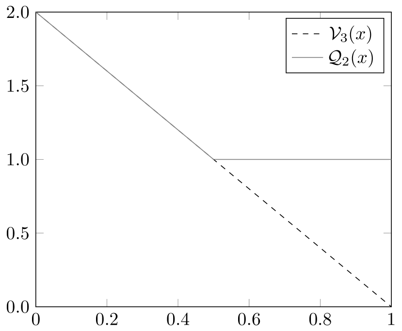
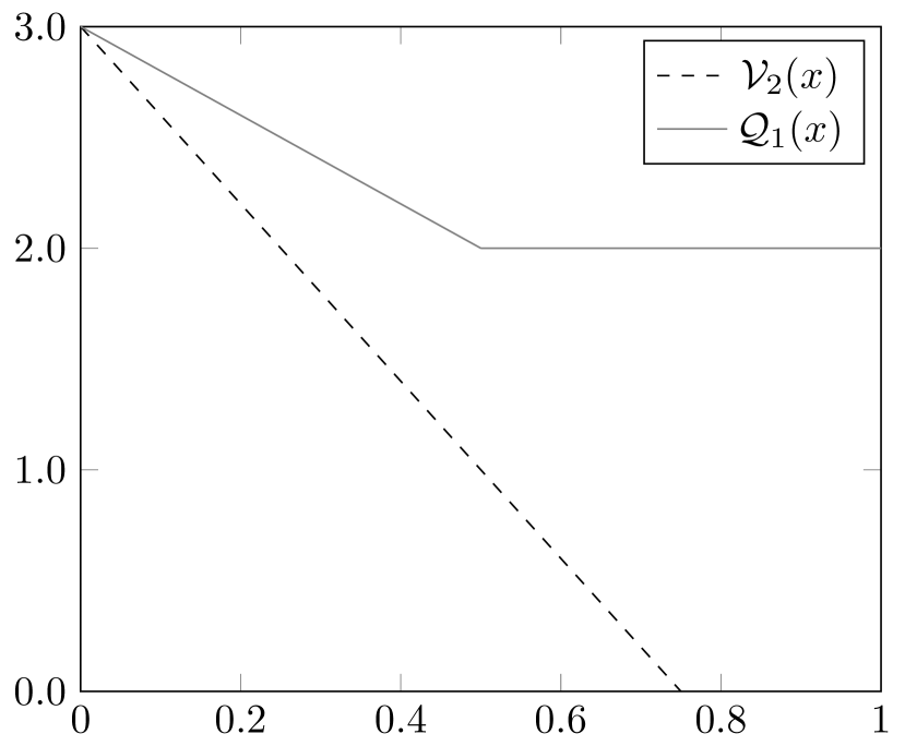
with . Note that if , the inner minimum value would be strictly smaller than (e.g., taking , , and ). Thus any optimal dual solution must satisfy as , , and gives an inner minimum value . By repeating the argument recursively, it can be checked that the under-approximation with . This implies that any optimal dual solution in stage would lie outside the open ball of radius , which is greater than 2, the Lipschitz constant of on . We illustrate the example with Figure 1 using .
2.3 Exactness of Dual Bounds
Example 2 suggests that the norm of optimal dual solutions for linear cut generation cannot be bounded by the Lipschitz constants of the value functions. Intuitively speaking, larger norms of dual variables lead to steeper linear cuts (6), which makes the under-approximation less useful at points away from the previously visited ones. For this reason, we propose to enforce bounds on the dual variables for recursive approximations and investigate the exactness of these artificial dual bounds. To begin with, let us fix algorithmic parameters for stages and define alternative value function recursively
| (10) |
with on and
| (11) |
for . We call them (Lipschitz) regularized value functions and (Lipschitz) regularized cost-to-go functions, due to the following observation.
Proposition 3.
For any and , the function is -Lipschitz continuous, and for all . Moreover, we can write as a value function
Proof.
We begin our proof for the equation with the following observation
Here, the first equality is due to Sion’s minimax theorem [23], where the maximization is taken over a compact ball of radius . The second equality follows from the dual representation of the norm functions [9, A.1.6]. The infimum is attained since the sum is bounded from below by our nonnegativity assumption of . Now it can be checked recursively for using the definition of that for any because is a feasible solution to the minimization.
It remains to show the -Lipschitz continuity of . Pick any and let denote the solutions in the minimization associated with for and , respectively. Then, as are also feasible solutions for the minimization associated with , we have
Now we can repeat the argument with exchanged indices 1 and 2 and show that , which completes the proof. ∎
We can now generate a linear cut using a dual solution and its associated infimum value of the following dual problem (cf. (6))
| (12) |
Whenever is an under-approximation of the regularized cost-to-go function , we can use the same argument as in (7) to see the validness of as a linear cut for , for all , and thus also the validness of as an aggregate linear cut for . The Lipschitz constants of these linear cuts and are bounded by .
By solving the bounded dual problems (12) for linear cut generation, by Proposition 3, we are essentially replacing the value functions and the cost-to-go functions with the regularized ones, and , respectively. We want to discuss that such replacement does not compromise any feasibility or optimality, which requires a technical lemma.
Lemma 2.
Let be a full-dimensional convex set and be a convex function. If the restriction is -Lipschitz continuous, then we have for any .
Proof.
Assume for contradiction that for some , there exists and such that . If lies in the interior , then we can find for some . Thus by convexity, , which contradicts the -Lipschitz continuity of .
Otherwise if , since is full-dimensional, we can find with , so . Besides, by the -Lipschitz continuity of , we have . Therefore,
which shows contradiction by the argument above since . ∎
Proposition 4.
Suppose that the state spaces are full-dimensional. If the value function is -Lipschitz continuous for any and , then we have for all and .
Proof.
Proposition 4 ensures the exactness of the bounded dual recursion (10) and (11), provided that the value functions are -Lipschitz continuous for some known values . We remark that the idea of bounding the dual variables, or equivalently adding a regularization term in the dual problems, could work more generally for multistage stochastic problems without RCR, and refer any interested readers to the paper [42].
3 Algorithms and Complexity Analysis
In this section, we first define single stage subproblem oracles (SSSO) for DR-MCO (1), based on which we define the notion of complexity of the algorithms. A simple implementation of the SSSO is then discussed for the finitely supported problems. We generalize the consecutive DDP (CDDP) algorithm to DR-MCO and more importantly, we introduce a new nonconsecutive DDP algorithm (NDDP). The complexity upper bound for each algorithm is then presented, and finally we provide a complexity lower bound for both algorithms, which shows the upper complexity bounds are nearly tight.
3.1 Single Stage Subproblem Oracles
A subproblem oracle is an oracle that gives a solution to the subproblem given its own information as well as the data generated by the algorithm. The single stage subproblem oracles (SSSO) used in this paper solve an approximation of the problem defined by (10) and (11) for some stage .
Definition 1 (Initial stage subproblem oracle).
Let denote two lsc, convex functions, with for any . Consider the following subproblem for the first stage ,
| (I) |
The initial stage subproblem oracle provides an optimal solution to (I) and calculates the approximation gap . We thus define the subproblem oracle formally as a map .
Definition 2 (Noninitial stage subproblem oracle).
For any , let denote two lsc, convex functions, with for all . Then given a feasible state , the stage- subproblem oracle provides a feasible state , an -Lipschitz continuous linear cut , and an over-estimate value such that
-
•
they are valid, i.e., on and ;
-
•
the gap is controlled, i.e., .
We thus define the subproblem oracle formally as a map .
The noninitial stage subproblem oracles are different from the initial stage subproblem oracle, in the sense that it does not necessarily provide any optimal solution to some optimization problem. Instead, it provides some feasible state, which could be used for exploration of the following stages, a linear cut and an estimate value for updating the approximation in the previous stages. As implementations for Definition 2 may be less intuitive than those for Definition 1, we provide some illustration using finitely supported DR-MCO below.
3.1.1 SSSO Implementation for Finitely Supported DR-MCO
We now propose a possible realization of the noninitial stage subproblem oracle based on the linear cut generation procedure discussed in Section 2.2. Suppose for each . By solving the bounded Lagrangian dual problem (12) for each , we can get primal solutions , , and linear cuts for that are all -Lipschitz continuous. We then aggregate them using , where is a maximizer at the given state . It is clear that is also -Lipschitz continuous. Next we solve the maximization problem
| (13) |
Note that by assumption for all , and is a feasible solution to the problem
Thus the value is a valid overestimation.
It remains to determine the feasible state and calculate the gap that satisfy the second requirement in Definition 2. Let for each . We pick the index corresponding to the largest gap , and set , . Consequently, we have
We summarize the above realization of the noninitial stage subproblem oracles in Algorithm 1.
We remark that Algorithm 1 is not the only way to realize the SSSO in Definition 2. For example, it is discussed in [17] that a polyhedral single stage subproblem of MRCO can be reformulated as mixed-integer linear optimization, which may then be solved by branch-and-bound type algorithms. Therefore, the introduction of SSSO may benefit our discussion by avoiding restrictions of solution methods in each stage, even when the uncertainty sets are finite. Besides, with SSSO, the complexity analysis may better reflect the computation time as the for-loop in Algorithm 1 can be easily parallelized. We also show in the next section that SSSO enables us to introduce a nonconsecutive dual dynamic programming algorithm.
3.2 Dual Dynamic Programming Algorithms
With the subproblem oracles, we generalize the consecutive dual dynamic programming (CDDP) algorithm to DR-MCO and introduce a nonconsecutive dual dynamic programming (NDDP) algorithm. Both algorithms produce deterministic upper bounds for exploration and termination.
3.2.1 Consecutive Dual Dynamic Programming
To ease the notation, we use to denote the function corresponding to the closed convex hull of the epigraphs of functions and . More precisely, we define
Note that if are further polyhedral, then by linear optimization strong duality, the function (assuming it is proper) can be written as
For each iteration , the main loop of CDDP (Algorithm 2) consists of three steps. The forward step uses the state in the previous stage and the approximations and to produce a new state . Then the backward step at stage uses the cut and the value to update the approximations in its precedent stage . The initial stage step produces a first stage solution and updates the lower and upper bounds.
We next discuss the correctness of Algorithm 2, i.e., the returned solution is -optimal as defined in (5), while leaving the finiteness proof to Section 3.3. From the termination of the while-loop, it suffices to show that the approximations are valid for each and . The first inequality follows from the validness of linear cuts (Definition 2). The second inequality is due to the -Lipschitz continuity of (Proposition 3). In particular, the inequality implies for all . Given that for , which is obviously true for , we conclude that
By taking the closed convex hull of the epigraphs on both sides, we have shown that for all . The above argument shows inductively that for all , the approximations are valid, which then implies the correctness of the algorithm.
We comment that the linear cut and the over-estimate value are generated using only the information in the previous iteration . In fact, the subproblem oracles can be re-evaluated in the backward steps to produce tighter approximations. We simply keep the CDDP algorithm in its current form because it is already sufficient for us to prove its complexity bounds, and hence its convergence. Alternatively, we propose a nonconsecutive version, NDDP, algorithm that could conduct more efficient approximation updates.
3.2.2 Nonconsecutive Dual Dynamic Programming
We describe the NDDP algorithm in Algorithm 3. To start the algorithm, it requires an additionally chosen vector of approximation gaps such that , compared with the CDDP algorithm. These predetermined approximation gaps serve as criteria at stage for deciding the next stage to be solved: the precedent stage or the subsequent one . If the algorithm decides to proceed to the subsequent stage , then the current state is used; otherwise the generated linear cut and over-estimate value are used for updating the approximations. The above argument of validness of approximations imply that for all holds for any stage and any index . Therefore, when NDDP terminates, the returned solution is indeed -optimal.
3.3 Complexity Upper Bounds
In this section, we provide a complexity analysis for the proposed CDDP and NDDP algorithms, which implies that both algorithms terminate in finite time for any finite and . Our goal is to derive an upper bound on the total number of subproblem oracle evaluations before the termination of the algorithm. To begin with, let , denote the set of pairs of indices such that the noninitial stage subproblem oracle is evaluated at the -th time at the state , i.e., . For the CDDP algorithm, all stages share the same iteration index , so for all . We define the following sets of indices for each :
| (14) |
Here, for NDDP algorithm, is the given approximation gap vector, while for CDDP algorithm, can be any vector satisfying for the purpose of analysis, since it is not required for the CDDP algorithm. We adopt the convention that the gap for the last stage such that if and only if and . In plain words, contains the pairs of indices where the state has an approximation gap greater than at -th evaluation, but at -th iteration the stage- oracle finds a solution with approximation gap smaller than . An important observation is that all these index sets are finite (before algorithm termination) , which is more precisely stated in the following lemma.
Lemma 3.
For stage any , suppose the state space is contained in a ball with diameter . Then,
| (15) |
Proof.
We claim that for any , , it holds that . Assume for contradiction that for some , . By definition of , the -th subproblem oracle is evaluated at the state , and in both the CDDP and the NDDP algorithms, the approximations and are updated since for some with . Then by Definition 2 of the noninitial stage subproblem oracle, we have . Note that for any point with , we have because of the -Lipschitz continuity of the approximations. Since and , by setting , we see a contradiction with the assumption that , which proves the claim.
To ease the notation, let denote the radius of the -dimensional balls centered at for , and let denote a ball with diameter . From the above claim, we know that for any with . In other words, the smaller balls are disjoint. Meanwhile, note that each of these smaller balls satisfies (the Minkowski sum in the Euclidean space ). Therefore, the volumes satisfy the relation
which implies that
∎
We prove the following complexity upper bounds for the CDDP algorithm (Theorem 1) and the NDDP algorithm (Theorem 2).
Theorem 1.
Suppose the state spaces are contained in balls, each with diameter . Then for the CDDP algorithm (Algorithm 2), the total number of subproblem oracle evaluations before termination is bounded by
Proof.
We prove by showing that for any approximation gap vector satisfying , the largest iteration index is bounded by
| (16) |
We claim that each iteration must lie in either of the following two cases:
-
1.
the initial stage step has ; or
-
2.
the -th forward step is in the index set for some stage .
To see the claim, suppose that the iteration is not in the first case. Then we have and by convention . Therefore, there exists a stage such that while , which is the second case. Note that when the first case happens, we have and thus the CDDP algorithm terminates. By Lemma 3, the second case can only happen at most times, proving the bound (16). The theorem then follows from the fact that in each CDDP iteration, the subproblem oracle is evaluated times with the additional evaluation of the initial stage subproblem oracle for checking the termination criterion. ∎
Remark 1.
When , , and for all , the bound in Theorem 1 can be simplified nicely. Note that the function
is strictly convex and symmetric under permutation on the simplex . Therefore, it has a unique optimal solution , which implies the infimum in (16) is attained by , . In this case, the CDDP complexity upper bound in Theorem 1 becomes
Theorem 2.
Suppose the state spaces are contained in balls, each with diameter . Then, for the NDDP algorithm (Algorithm 3) with the predetermined approximation gap vector satisfying , the total number of subproblem oracle evaluations before termination is bounded by
Proof.
For the NDDP algorithm, each time when it decides to go back to the precedent stage , we must have while for some . In this case, we have by definition that . By Lemma 3, such “going back” steps can only happen at most times. The total number of evaluations is then bounded by two times the number of “going back” steps due to the corresponding “going forward” steps, plus an additional evaluation of the initial stage oracle for checking the termination criterion. ∎
Let us compare the complexity bounds of the two algorithms. If we fix the approximation gap vector in Theorem 1 to be the same in the NDDP algorithm, then the complexity bound of CDDP grows faster than that of NDDP as . However, since an optimal choice of the gap vector is usually not known, CDDP has the advantage of not requiring estimates of these factors for the algorithm to be executed.
In many practical problems, it is reasonable to allow the target optimality gap to grow with . We say is an -relative optimal solution if
An -optimal first stage solution is -relative optimal if
We provide below an important simplification of the above complexity bounds when considering relative optimality gaps.
Corollary 1.
Suppose that all the state spaces have the same dimension and are bounded by a common diameter , and let . If for each stage , the local cost functions are uniformly bounded from below by for all feasible solutions and uncertainty outcomes , i.e., , then the total number of subproblem oracle evaluations before achieving an -relative optimal solution for CDDP and NDDP are upper bounded respectively by
Proof.
Corollary 1 shows that for problems that have strictly positive cost in each stage, the proposed complexity bounds for an -relative optimal solution grow at most quadratically for CDDP and linearly for NDDP with respect to the number of stages . At the same time, they both grow exponentially with the dimension . In what follows, we show that this exponential dependence on is nearly tight by providing a matching lower bound.
3.4 Complexity Lower Bound
Note that if we take for , then the complexity upper bounds in Theorems 1 and 2 depend on terms or , where is the state space dimension of stage . It is natural to ask whether it is possible for either algorithm to achieve an -optimal solution without the exponential dependence on the state space dimensions as in Corollary 1. We construct a class of convex problems to show that this is indeed impossible.
Given a -sphere with radius , a spherical cap with depth centered at a point is the set . Our construction is based on the following technical lemma, where we use to denote the gamma function.
Lemma 4 ([42, Lemmas 8 and 9]).
Given a -sphere and depth , there exists a finite set of points with
such that for any , . Moreover, given a positive constant , any function can be extended to an -Lipschitz continuous convex function , such that is differentiable at any point of , and the approximate functions
satisfy and .
We next construct a class of deterministic DR-MCO problems using such convex functions, with the following parameters: as the number of stages, as an upper bound on Lipschitz constants, as the state space dimension, as the state space diameter, and as the target optimality gap. Set . Construct sets of points , where for . Let be an -Lipschitz continuous convex function on constructed in Lemma 4 with for each . And we denote . Our DR-MCO problems for the complexity lower bound are defined by the following recursions for
| (17) |
where , and the first stage problem is defined as . We assume that the dual bounds satisfy , for the exactness guaranteed by Proposition 4. To describe the asymptotic behavior of a lower bound, we use the -notation, i.e., for functions , if .
Theorem 3.
Proof.
We assume that our SSSO at stage returns points in in the first evaluations without repetition. More specifically, for and , given and at some , the SSSO returns
-
•
a state with for all ;
-
•
a linear cut ;
-
•
an overestimate .
where for any . Thus our under- and over-approximations of can be written as
To see that the above assumption on the SSSO does not conflict with Definition 2, it is straightforward to check that the state is feasible, the overestimate , and the gap is controlled . For the validness of the linear cut , note that by Lemma 4, for all . Thus by a recursive argument from to , we know that when for all . Similarly, one can verify that . Therefore, . In other words, when the algorithms terminate, we must have for some , which implies
Here, the last inequality is due to Wendel’s bound on the ratio of two gamma functions [34]. ∎
Remark 2.
The CDDP and NDDP algorithms (Algorithms 2 and 3) and their complexity analyses depend only on the SSSO (Definitions 1 and 2). Therefore, while we only discuss SSSO implementations for finitely supported DR-MCO in Section 3.1.1, the CDDP and NDDP algorithms work for more general DR-MCO problems. Moreover, the complexity upper bounds (Theorems 1 and 2, Corollary 1) and the lower bound (Theorem 3) remain valid for them as well.
4 Numerical Experiments
In this section, we numerically test the proposed CDDP and NDDP algorithms. The first test problem is a robust multi-commodity inventory problem with customer demand uncertainty. The second test problem is a distributionally robust hydro-thermal power planning problem with stochastic energy inflows. The computation budget consists of 10 3.0-GHz CPU cores and a total of 70 GBytes of RAM. The algorithms are implemented using JuMP package ([13], v1.14) in Julia language (v1.9) with Gurobi 9.5 [20] as its underlying LP solver.
4.1 Multi-Commodity Inventory Problem
We consider an MRCO of multi-commodity inventory problem with uncertain customer demands and deterministic holding and backlogging costs, following the description in [17]. This problem can be described through the local cost functions and the uncertainty sets . Let denote the set of product indices. We first describe the variables in each stage . We use to denote the inventory level, (resp. ) to denote the amount of express (resp. standard) order fulfilled in the current (resp. subsequent) stage, of some product . Let denote the uncertainty vector controlling the customer demands in stage . The state variables consist of the collection , while the internal variables are simply the express order amounts . In stage , the local cost function and the state space are defined by
| (18) | |||||
and
| (19) |
Here in the formulation, (resp. ) denotes the express (resp. standard) order unit cost, (resp. ) the inventory holding (resp. backlogging) unit cost, (resp. ) the bound on the express (resp. standard) order, and the inventory level bound, for the product , respectively. The first constraint in (18) is a cumulative bound on the express orders, the second constraint characterizes the change in the inventory level, and the last of (18) and the state space (19) represent bounds on the decision variables with respect to each product. We also put as a fixed cost to ensure the cost function is strictly positive (cf. Corollary 1). We use and to denote the positive and negative part of a real number . The initial state is given by for all . The uncertainty set is an -dimensional box , and the customer demand is predicted by the following factor model:
| (20) |
where is an -dimensional vector where each entry is chosen uniformly at random from . Thus the value and for all and .
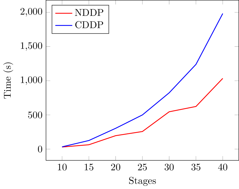
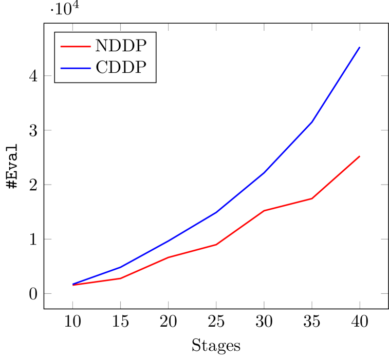
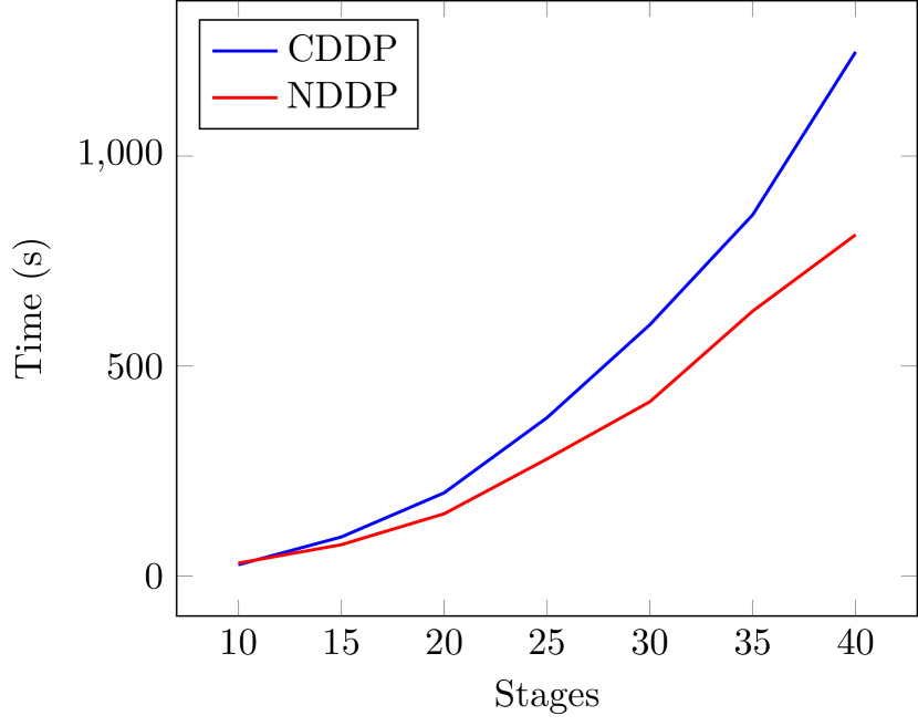
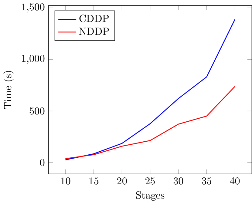
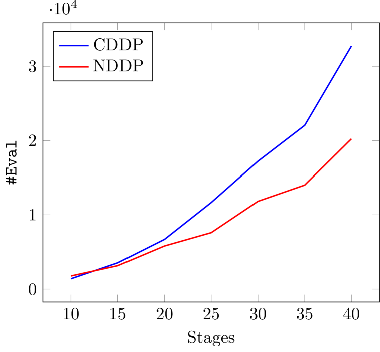
For the following numerical test, we set the number of products , the number of uncertainty factors , , for all , , and . The costs are generated uniformly at random within , for all . Due to lack of RCR of the problem (18), we first test both CDDP (Algorithm 2) and NDDP (Algorithm 3) with dual bounds for all . The optimality gap set to be relative and approximation gaps set dynamically by for . Over 3 independently generated test cases, we plot the growth of computational time and number of oracle evaluations with respect to the number of stages in Fig. 2, which shows that NDDP performs increasingly better than CDDP as the number of stages increases. In particular, NDDP can save up to 47.8% computation time and up to 44.2% subproblem oracle evaluations comparing to CDDP for these 40-stage problems.

As a comparison, we implement the NDDP algorithm without dual bounds. Instead, it generates linear feasibility cuts for approximation of the feasible sets (see definition of feasibility cuts in, e.g., [19]). We limit the computational budget to subproblem oracle calls. For 5 independently generated test cases, we have obtained the following results (Table 1).
| With Dual Bounds | Without Dual Bounds | |||||||
|---|---|---|---|---|---|---|---|---|
| Stage | LB | UB | Time (s) | #Eval | LB | UB | Time (s) | #Eval |
| 10 | 154.70 | 156.02 | 30.61 | 1554 | 154.70 | 155.30 | 33.34 | 1497 |
| 155.98 | 157.06 | 30.80 | 1523 | 155.98 | 157.37 | 14.16 | 1371 | |
| 128.33 | 128.89 | 37.33 | 1771 | 128.31 | 129.48 | 19.46 | 1803 | |
| 137.06 | 137.16 | 26.69 | 1355 | 137.06 | 137.06 | 14.75 | 1397 | |
| 120.12 | 120.82 | 70.06 | 2345 | 118.11 | inf | 318.05 | 20003 | |
| 15 | 232.46 | 233.85 | 63.84 | 2776 | 232.13 | inf | 440.07 | 30037 |
| 233.38 | 235.56 | 74.51 | 3104 | 233.58 | 235.23 | 33.90 | 2891 | |
| 202.31 | 203.40 | 75.25 | 3154 | 202.48 | 203.70 | 40.89 | 3522 | |
| 208.56 | 210.14 | 61.55 | 2707 | 208.50 | 209.28 | 33.85 | 2900 | |
| 195.16 | 196.78 | 129.38 | 4589 | 191.30 | inf | 666.52 | 30024 | |
| 20 | 291.78 | 293.94 | 196.57 | 6637 | 286.88 | inf | 615.68 | 40054 |
| 292.87 | 295.77 | 148.18 | 5561 | 292.87 | 293.14 | 67.45 | 4955 | |
| 256.15 | 258.03 | 157.78 | 5810 | 256.19 | 258.63 | 74.12 | 5762 | |
| 261.81 | 263.80 | 113.54 | 4569 | 261.81 | 261.82 | 61.22 | 4821 | |
| 249.85 | 252.26 | 277.24 | 8296 | 235.01 | inf | 665.76 | 40002 | |
| 25 | 369.62 | 372.54 | 257.33 | 8984 | 369.66 | 371.10 | 102.86 | 7334 |
| 370.08 | 373.74 | 278.66 | 9225 | 370.47 | 371.39 | 101.37 | 7153 | |
| 330.18 | 333.38 | 213.01 | 7602 | 330.37 | 331.63 | 112.88 | 8133 | |
| 333.20 | 336.05 | 166.87 | 6346 | 333.34 | 333.74 | 96.10 | 6946 | |
| 324.83 | 327.99 | 479.58 | 12785 | 323.43 | inf | 1167.04 | 50006 | |
| 30 | 428.81 | 432.41 | 545.98 | 15212 | 429.11 | 429.69 | 165.55 | 10217 |
| 429.34 | 432.08 | 414.91 | 12639 | 429.77 | 430.27 | 141.67 | 9549 | |
| 383.74 | 387.01 | 372.00 | 11820 | 384.22 | 387.43 | 173.06 | 11368 | |
| 386.54 | 390.41 | 277.57 | 9430 | 386.56 | 386.58 | 151.97 | 9824 | |
| 379.46 | 382.84 | 649.69 | 16730 | 379.27 | inf | 1230.98 | 60016 | |
In Table 1, the inf indicates values of infinity or numerically infinity values (i.e., values greater than ) upon termination. As we see from the table, the NDDP algorithm together with feasibility cuts fails to solve 2 out of 5 cases even when there are only 15 stages, showing the instability of the performance of feasibility cuts. In contrast, the algorithm with the dual-bounding technique solves all of the cases within a reasonable computation time and number of subproblem oracle evaluations, without any optimality gap on those cases that both formulations are able to solve. This demonstrates the ability of the our proposed DDP algorithms handling problems without RCR. It is worth mentioning that for cases where the NDDP algorithm converges without dual bounds, the computation time used is usually smaller than the regularized problem, which can be explained by better numerical conditions of feasibility cuts and their effect on reducing the effective volumes of the state space.
4.2 Hydro-Thermal Power Planning Problem
We next consider the Brazilian interconnected power system described in [12]. By assuming the stagewise independence and taking sample average approximation in the underlying stochastic energy inflow, we formulate the problem below as a finitely supported DR-MCO (1). Let denote the indices of regions in the system ( in our data), and the indices of thermal power plants, where each of the disjoint subsets is associated with the region . We first describe the decision variables in each stage . Let denote the finite uncertainty set of energy inflow in stage . We use to denote the stored energy level, to denote the hydro power generation, and to denote the energy spillage, of some region ; and to denote the thermal power generation for some thermal power plant . For two different regions , we use to denote the energy exchange from region to region , and to denote the deficit account for region in region . Let be the state variables and denote the internal variables consisting of , and for any and . Then in stage , the state space is simply , and the local cost function can be defined as
| (21) | |||||
Here in the formulation, denotes the unit penalty on energy spillage, the unit cost of thermal power generation of plant , the unit cost of power exchange from region to region , the unit cost on the energy deficit account for region in region , the deterministic power demand in stage and region , the bound on the storage level in region , the bound on hydro power generation in region , the lower and upper bounds of thermal power generation in plant , the bound on the deficit account for region in region , and the bound on the energy exchange from region to region . The first constraint in (21) characterizes the change of energy storage levels in each region , the second constraint imposes the power generation-demand balance for each region , and the rest are bounds on the decision variables. The initial state and are given by data.
The energy inflow outcomes are sampled from multivariate lognormal distributions that are interstage independent. Then the distributional ambiguity set is constructed using Wasserstein metric to reduce the effect of overtraining with the sampled outcome, according to [14]. To be precise, suppose is an empirical distribution of outcomes . Then, the distributional ambiguity set is described by
| (22) |
for some radius , where the Wasserstein metric for finitely supported distributions is defined by
| (23) | |||||
Note when the radius , the ambiguity set becomes a singleton. In our numerical tests, we choose the radius to be relative to the total distances, i.e., for some . At the same time, we use uniform dual bounds for the tests, i.e., for all . When the relative optimality gap is smaller than the threshold , we check whether all the active cuts in the recent iterations are strictly smaller than the regularization factor. If they are, then the algorithm is terminated, and otherwise the dual bound is increased by a factor of with all the over-approximations reset to , . Five scenarios are sampled independently in each stage for the nominal problem before the distributional robust counterpart is constructed by (22). For the 24-stage problem that we consider, the samples already give a total scenario paths, which is already impossible to solve via an extensive formulation. We have then obtained the following results (Table 2).
| LB () | UB () | Med. Time (s) | Med. #Eval | ||
|---|---|---|---|---|---|
| 0.00 | 2 | 4.60 | 4.84 | 784.45 | 33075 |
| 3 | 4.59 | 4.83 | 301.06 | 15345 | |
| 4 | 4.58 | 4.82 | 374.88 | 17505 | |
| 5 | 4.58 | 4.82 | 378.80 | 17595 | |
| 6 | 4.58 | 4.82 | 386.86 | 17910 | |
| 0.02 | 2 | 4.84 | 5.09 | 439.28 | 22095 |
| 3 | 4.84 | 5.09 | 263.26 | 13725 | |
| 4 | 4.82 | 5.07 | 365.72 | 17100 | |
| 5 | 4.82 | 5.07 | 358.08 | 16830 | |
| 6 | 4.82 | 5.07 | 405.42 | 18090 | |
| 0.04 | 2 | 5.10 | 5.36 | 921.99 | 36720 |
| 3 | 5.06 | 5.32 | 237.34 | 13095 | |
| 4 | 5.06 | 5.33 | 327.38 | 15975 | |
| 5 | 5.06 | 5.33 | 325.62 | 15930 | |
| 6 | 5.06 | 5.33 | 350.65 | 16650 | |
| 0.06 | 2 | 5.34 | 5.62 | 606.61 | 27810 |
| 3 | 5.32 | 5.60 | 284.40 | 14445 | |
| 4 | 5.31 | 5.59 | 277.21 | 14310 | |
| 5 | 5.30 | 5.58 | 271.26 | 14130 | |
| 6 | 5.31 | 5.59 | 285.30 | 14445 | |
| 0.08 | 2 | 5.57 | 5.86 | 519.87 | 25380 |
| 3 | 5.55 | 5.84 | 204.36 | 11790 | |
| 4 | 5.54 | 5.83 | 290.96 | 14715 | |
| 5 | 5.54 | 5.83 | 223.92 | 12510 | |
| 6 | 5.54 | 5.83 | 257.26 | 13500 | |
| 0.10 | 2 | 5.81 | 6.12 | 446.94 | 22140 |
| 3 | 5.78 | 6.08 | 194.85 | 10980 | |
| 4 | 5.78 | 6.09 | 262.42 | 12915 | |
| 5 | 5.78 | 6.09 | 215.10 | 11790 | |
| 6 | 5.79 | 6.09 | 237.22 | 12420 |
In Table 2, the lower bound (LB), the upper bound (UB) at termination, the computation time (Med. Time) and the number of subproblem oracles (Med. #Eval) shown are the median of the five test cases. The logarithmic regularization factors listed in the table correspond to the initial regularization factors. We see that for different choices of the relative radii , the median computation time and number of subproblem oracle evaluations are usually smaller when , without compromising the quality of upper and lower bounds. This can be explained by the better numerical conditions for the smaller regularization factors (the cuts have smaller Lipschitz constants), leading to shorter subproblem oracle evaluations times (cf. Algorithm 1). We thus conclude that the regularization technique could lead to smaller number of subproblem oracle evaluations, as well as shorter computation time for a given DR-MCO problem.
5 Concluding Remarks
In this work, we extend CDDP algorithms to a broad class of DR-MCO problems, and propose a novel NDDP algorithm that decides its stage exploration strategy dynamically based on the cost-to-go function approximation qualities. We enforce bounds on the DDP recursion dual variables to effectively control the growth of Lipschitz constants in the approximation. We provide a comprehensive complexity analysis of both CDDP and NDDP algorithms, proving both upper complexity bounds and a matching lower bound, which reveal, in a precise way, the dependence of the complexity of the DDP-type algorithms on the number of stages, the dimension of the decision space, and various regularity characteristics of DR-MCO. In particular, our NDDP algorithm scales linearly with , assuming that the target optimality gap scales with . This is the first complexity analysis of DDP-type algorithms in such a general setting, and we believe it provides key insights for further developing efficient computational tools for the very many applications of sequential decision making under uncertainty. We also provide numerical examples to show the capability of the DDP-type algorithms method to solve problems without RCR, and reduction in computation time and number of subproblem oracle evaluations, due to the dual-bounding technique.
References
- Ahmed et al. [2019] S Ahmed, F G Cabral, and B F Paulo da Costa. Stochastic lipschitz dynamic programming, 2019.
- Anderson and Philpott [2019] E J Anderson and A B Philpott. Improving sample average approximation using distributional robustness. Optimization Online, 2019.
- Baucke et al. [2017] R Baucke, A Downward, and G Zakeri. A deterministic algorithm for solving multistage stochastic programming problems. Optimization Online, 2017.
- Baucke et al. [2018] R Baucke, A Downward, and G Zakeri. A deterministic algorithm for solving stochastic minimax dynamic programmes. Optimization Online, 2018.
- Bauschke et al. [2011] Heinz H Bauschke, Patrick L Combettes, et al. Convex analysis and monotone operator theory in Hilbert spaces, volume 408. Springer, 2011.
- Ben-Tal et al. [2009] A Ben-Tal, L El Ghaoui, and A Nemirovski. Robust optimization, volume 28. Princeton University Press, 2009.
- Bertsimas and Georghiou [2015] D Bertsimas and A Georghiou. Design of near optimal decision rules in multistage adaptive mixed-integer optimization. Operations Research, 63(3):610–627, 2015.
- Birge [1985] John R. Birge. Decomposition and Partitioning Methods for Multistage Stochastic Linear Programs. Operations Research, 33(5):989–1007, October 1985. ISSN 0030-364X, 1526-5463. doi: 10.1287/opre.33.5.989.
- Boyd et al. [2004] Stephen Boyd, Stephen P Boyd, and Lieven Vandenberghe. Convex optimization. Cambridge university press, 2004.
- Chen and Powell [1999] Z L Chen and W B Powell. Convergent Cutting-Plane and Partial-Sampling Algorithm for Multistage Stochastic Linear Programs with Recourse. Journal of Optimization Theory and Applications, 102(3):497–524, September 1999. ISSN 0022-3239, 1573-2878. doi: 10.1023/A:1022641805263.
- de Matos et al. [2015] Vitor L. de Matos, Andy B. Philpott, and Erlon C. Finardi. Improving the performance of Stochastic Dual Dynamic Programming. Journal of Computational and Applied Mathematics, 290:196–208, December 2015. ISSN 03770427. doi: 10.1016/j.cam.2015.04.048.
- Ding et al. [2019] L Ding, S Ahmed, and A Shapiro. A python package for multi-stage stochastic programming. Optimization Online, pages 1–41, 2019.
- Dunning et al. [2017] I Dunning, J Huchette, and M Lubin. Jump: A modeling language for mathematical optimization. SIAM Review, 59(2):295–320, 2017. doi: 10.1137/15M1020575.
- Duque and Morton [2019] D Duque and D P Morton. Distributionally robust stochastic dual dynamic programming. Optimization Online, 2019.
- Dyer and Stougie [2006] Martin Dyer and Leen Stougie. Computational complexity of stochastic programming problems. Mathematical Programming, 106(3):423–432, May 2006. ISSN 0025-5610, 1436-4646. doi: 10.1007/s10107-005-0597-0.
- Flach et al. [2010] B.C. Flach, L.A. Barroso, and M.V.F. Pereira. Long-term optimal allocation of hydro generation for a price-maker company in a competitive market: Latest developments and a stochastic dual dynamic programming approach. IET Generation, Transmission & Distribution, 4(2):299, 2010. ISSN 17518687. doi: 10.1049/iet-gtd.2009.0107.
- Georghiou et al. [2019] A Georghiou, A Tsoukalas, and W Wiesemann. Robust dual dynamic programming. Operations Research, 67(3):813–830, 2019.
- Girardeau et al. [2015] P. Girardeau, V. Leclere, and A. B. Philpott. On the Convergence of Decomposition Methods for Multistage Stochastic Convex Programs. Mathematics of Operations Research, 40(1):130–145, February 2015. ISSN 0364-765X, 1526-5471. doi: 10.1287/moor.2014.0664.
- Grothey et al. [1999] A Grothey, S Leyffer, and KIM McKinnon. A note on feasibility in benders decomposition. Numerical Analysis Report NA/188, Dundee University, 1999.
- Gurobi Optimization, LLC [2023] Gurobi Optimization, LLC. Gurobi Optimizer Reference Manual, 2023. URL https://www.gurobi.com.
- Hadjiyiannis et al. [2011] M J Hadjiyiannis, P J Goulart, and D Kuhn. A scenario approach for estimating the suboptimality of linear decision rules in two-stage robust optimization. In 2011 50th IEEE Conference on Decision and Control and European Control Conference, pages 7386–7391. IEEE, 2011.
- Huang et al. [2017] J Huang, K Zhou, and Y Guan. A Study of Distributionally Robust Multistage Stochastic Optimization. arXiv:1708.07930 [math], August 2017.
- Komiya [1988] Hidetoshi Komiya. Elementary proof for sion’s minimax theorem. Kodai mathematical journal, 11(1):5–7, 1988.
- Kuhn et al. [2011] D Kuhn, W Wiesemann, and A Georghiou. Primal and dual linear decision rules in stochastic and robust optimization. Mathematical Programming, 130(1):177–209, 2011.
- Lan [2019] Guanghui Lan. Complexity of Stochastic Dual Dynamic Programming. arXiv:1912.07702, December 2019.
- Linowsky and Philpott [2005] K. Linowsky and A. B. Philpott. On the Convergence of Sampling-Based Decomposition Algorithms for Multistage Stochastic Programs. Journal of Optimization Theory and Applications, 125(2):349–366, May 2005. ISSN 0022-3239, 1573-2878. doi: 10.1007/s10957-004-1842-z.
- Liu [2019] R P Liu. On feasibility of sample average approximation solutions to stochastic programming. arXiv preprint arXiv:1904.00137, 2019.
- Pereira and Pinto [1985] M. V. F. Pereira and L. M. V. G. Pinto. Stochastic Optimization of a Multireservoir Hydroelectric System: A Decomposition Approach. Water Resources Research, 21(6):779–792, June 1985. ISSN 00431397. doi: 10.1029/WR021i006p00779.
- Pereira and Pinto [1991] M. V. F. Pereira and L. M. V. G. Pinto. Multi-stage stochastic optimization applied to energy planning. Mathematical Programming, 52(1-3):359–375, May 1991. ISSN 0025-5610, 1436-4646. doi: 10.1007/BF01582895.
- Philpott et al. [2019] A Philpott, F Wahid, and F Bonnans. MIDAS: a mixed integer dynamic approximation scheme. Mathematical Programming, pages 1–32, 2019.
- Philpott et al. [2018] A. B. Philpott, V. L. de Matos, and L. Kapelevich. Distributionally robust SDDP. Computational Management Science, 15(3-4):431–454, October 2018. ISSN 1619-697X, 1619-6988. doi: 10.1007/s10287-018-0314-0.
- Philpott and Guan [2008] A.B. Philpott and Z. Guan. On the convergence of stochastic dual dynamic programming and related methods. Operations Research Letters, 36(4):450–455, July 2008. ISSN 01676377. doi: 10.1016/j.orl.2008.01.013.
- Philpott et al. [2013] Andy Philpott, Vitor de Matos, and Erlon Finardi. On Solving Multistage Stochastic Programs with Coherent Risk Measures. Operations Research, 61(4):957–970, August 2013. ISSN 0030-364X, 1526-5463. doi: 10.1287/opre.2013.1175.
- Qi [2010] Feng Qi. Bounds for the ratio of two gamma functions. Journal of Inequalities and Applications, 2010:1–84, 2010.
- Rudin [1987] Walter Rudin. Real and complex analysis. Tata McGraw-hill education, third edition, 1987.
- Shapiro [2006] A Shapiro. On complexity of multistage stochastic programs. OR Letters, 34(1):1–8, January 2006. ISSN 01676377. doi: 10.1016/j.orl.2005.02.003.
- Shapiro [2011] A Shapiro. Analysis of stochastic dual dynamic programming method. European Journal of Operational Research, 209(1):63–72, February 2011. ISSN 03772217. doi: 10.1016/j.ejor.2010.08.007.
- Shapiro and Ding [2019] A Shapiro and L Ding. Stationary multistage programs. Optimization Online, 2019.
- Shapiro et al. [2009] A Shapiro, D Dentcheva, and A Ruszczyński. Lectures on stochastic programming. SIAM, 2009.
- Shapiro et al. [2013] A Shapiro, W Tekaya, J P da Costa, and M P Soares. Risk neutral and risk averse Stochastic Dual Dynamic Programming method. European Journal of Operational Research, 224(2):375–391, January 2013. ISSN 03772217. doi: 10.1016/j.ejor.2012.08.022.
- Shapiro et al. [2012] Alexander Shapiro, Wajdi Tekaya, Joari P da Costa, and Murilo P Soares. Final report for technical cooperation between georgia institute of technology and ons–operador nacional do sistema elétrico. Georgia Tech ISyE Report, 2012.
- Zhang and Sun [2022] Shixuan Zhang and Xu Andy Sun. Stochastic dual dynamic programming for multistage stochastic mixed-integer nonlinear optimization. Mathematical Programming, 196(1):935–985, 2022.
- Zou et al. [2019a] J Zou, S Ahmed, and X A Sun. Stochastic dual dynamic integer programming. Mathematical Programming, 175(1-2):461–502, May 2019a. ISSN 0025-5610, 1436-4646. doi: 10.1007/s10107-018-1249-5.
- Zou et al. [2019b] Jikai Zou, Shabbir Ahmed, and Xu Andy Sun. Multistage Stochastic Unit Commitment Using Stochastic Dual Dynamic Integer Programming. IEEE Transactions on Power Systems, 34(3):1814–1823, May 2019b. ISSN 0885-8950, 1558-0679. doi: 10.1109/TPWRS.2018.2880996.