Variational Approximation of Factor Stochastic Volatility Models

Abstract

Estimation and prediction in high dimensional multivariate factor stochastic volatility models is an important and active research area because such models allow a parsimonious representation of multivariate stochastic volatility. Bayesian inference for factor stochastic volatility models is usually done by Markov chain Monte Carlo methods, often by particle Markov chain Monte Carlo, which are usually slow for high dimensional or long time series because of the large number of parameters and latent states involved. Our article makes two contributions. The first is to propose fast and accurate variational Bayes methods to approximate the posterior distribution of the states and parameters in factor stochastic volatility models. The second contribution is to extend this batch methodology to develop fast sequential variational updates for prediction as new observations arrive. The methods are applied to simulated and real datasets and shown to produce good approximate inference and prediction compared to the latest particle Markov chain Monte Carlo approaches, but are much faster.

Keywords: Bayesian Inference; Prediction; State space model; Stochastic gradient; Sequential variational inference.

1 Introduction

Statistical inference and prediction in high dimensional time series models that incorporate stochastic volatility (SV) is an important and active research area because of its applications in financial econometrics and financial decision making. One of the main challenges in estimating such models is that the number of parameters and latent variables involved often increases quadratically with dimension, while the length of each latent variable equals the number of time periods. These problems are lessened by using a factor stochastic volatility (FSV) model. See, e.g. Pitt and Shephard, (1999) and Chib et al., (2006) who use independent and low dimensional latent factors to approximate a fully multivariate SV (MSV) model to achieve an attractive tradeoff between model complexity and model flexibility.

Although FSV models are more tractable computationally than high dimensional multivariate SV (MSV) models, they are still challenging to estimate because they are relatively high dimensional in the number of parameters and latent state variables; the likelihood of any FSV model is also intractable as it is a high dimensional integral over the latent state variables. Current state of the art approaches use Markov chain Monte Carlo (MCMC) (e.g., Chib et al.,, 2006; Kastner et al.,, 2017) were developed over a number of years and are very powerful. However, they are less flexible and accurate than recent particle MCMC based approaches by Mendes et al., (2020), Li and Scharth, (2020) and Gunawan et al., (2020) as they use the approach proposed in Kim et al., (1998) (based on assuming normal errors) to approximate the distribution of the innovations in the log outcomes (usually the log of the squared returns) by a mixture of normals; see Mendes et al., (2020) for a comparison of the accuracy and flexibility of the Chib et al., (2006) approach compared to the particle MCMC approach. As well as estimating the FSV model, practitioners are often interested in updating estimates of the parameters and latent volatilities as new observations arrive, and obtaining one-step or multiple-steps ahead predictive distributions of future volatilities and observations. However, it is usually computationally very expensive to estimate a factor stochastic volatility by MCMC or particle MCMC. Sequential updating by MCMC or particle MCMC is even more expensive as it is necessary to carry out a new MCMC simulation as new observations become available, although such updating is made simpler because good starting values for the MCMC are available from the previous MCMC run. Sequential Monte Carlo methods can also be used instead for estimation and sequential updating, but these can also be expensive.

Variational Bayes (VB) has become increasingly prominent as a method for conducting parameter inference in a wide range of challenging statistical models with computationally difficult posteriors (Ormerod and Wand,, 2010; Tan and Nott,, 2018; Ong et al.,, 2018; Blei et al.,, 2017). VB expresses the estimation of the posterior distribution as an optimisation problem by approximating the posterior density by a simpler distribution whose parameters are unknown, e.g., by a multivariate Gaussian with unknown mean and covariance matrix. VB methods usually produce posterior inference with much less computational cost compared to the exact methods such as MCMC or particle MCMC, although they are approximate.

Our article makes two contributions. First, it proposes fast and accurate variational approximations of the posterior distribution of the latent volatilities and parameters of a multivariate factor stochastic volatility model. It does so by carefully studying which dependencies it is important to retain in the variational posterior to obtain good approximations; and which can be omitted, thus speeding up the computation. This results in approximate Bayesian inference that is very close to that obtained by the much slower particle methods.

The second contribution is to develop a sequential version of the batch approach in the first contribution which updates the variational approximation as new observations arrive. The sequential version can be used for one step and multiple steps forecasting as new observations arrive. It is also useful for time series cross-validation for model selection as well as assessing model fit. Sections 5.1 and 5.2 show that our variational approach produces forecasts that are very close to those obtained from the exact particle MCMC methods, even when the corresponding variational posterior variance is sometimes underestimated.

The importance of the second contribution is that the variational updates and forecasts are produced with much less computational cost compared to the time taken to produce the corresponding updates and exact predictions using particle MCMC.

Although our article focuses on a particular, but quite general, factor stochastic volatility model, we believe that the methodology developed can be applied to a wide range of such models. See Section 6 for further remarks.

The current VB literature focuses on a Gaussian VB for approximating the posterior density. The variational parameters to be optimised are the mean vector and the covariance matrix. It is challenging to perform Gaussian variational approximation with an unrestricted covariance matrix for high dimensional parameters because the number of elements in the covariance matrix of the variational density increases quadratically with number of model parameters. It is then very important to find an effective and efficient parameterisation of the covariance structure of the variational density when the number of latent states and parameters are large as in the multivariate factor SV model.

Various suggestions in the literature exist for parsimoniously parameterising the covariance matrix in the Gaussian variational approximation (GVA). Titsias and Lazaro-Gredilla, (2014) use a Cholesky factorisation of the full covariance matrix, but they do not allow for parameter sparsity; the exceptions are diagonal approximations which lose any ability to capture posterior dependence in the variational approximation. Kucukelbir et al., (2017) also consider an unrestricted and diagonal covariance matrix and use similar gradient estimates to Titsias and Lazaro-Gredilla, (2014), but use automatic differentiation. Tan and Nott, (2018) parameterise the precision matrix in terms of a sparse Cholesky factor that reflects the conditional independence structure in the model. This approach is motivated by the result that a zero on the off-diagonal in the precision matrix means that the corresponding two variables are conditionally independent (Tan and Nott,, 2018). The computations can then be done efficiently through fast sparse matrix operations. Recently, Ong et al., (2018) consider a factor covariance structure as a parsimonious representation of the covariance matrix in the Gaussian variational approximation. They also combine stochastic gradient ascent optimisation with the “reparameterisation trick’(Kingma and Welling,, 2014). Opper and Archambeau, (2009), Challis and Barber, (2013), and Salimans and Knowles, (2013) consider other parameterisations of the covariance matrix in the Gaussian variational approximation. Quiroz et al., (2018) combine the factor parameterisation and sparse precision Cholesky factors for capturing dynamic dependence structure in high-dimensional state space model. They apply their method to approximate the posterior density of the multivariate stochastic volatility model via a Wishart process. The computational cost of their variational approach increases with the length of the time series and their variational approach is currently limited to low dimensional and short time series. Our proposed variational approach is scalable in terms of number of parameters, latent states, and observations.

Tan et al., (2019) and Smith et al., (2019) propose more flexible variational approximations than GVA. Tan et al., (2019) extend the approach in Tan and Nott, (2018) by defining the posterior distribution as a product of two Gaussian densities. The first is the posterior for the global parameters; the second is the posterior of the local parameters, conditional on the global parameters. The method respects a conditional independence structure similar to that of Tan and Nott, (2018), but allows the joint posterior to be non-Gaussian because the conditional mean of the local parameters can be nonlinear in the global parameters. Similarly to Tan and Nott, (2018), they also exploit the conditional independence structure in the model and improve the approximation by using the importance weights approach (Burda et al.,, 2016). Smith et al., (2019) propose an approximation that is based on implicit copula models for original parameters with a Gaussian or skew-normal copula function and flexible parametric marginals. They consider the Yeo-Johnson (Yeo and Johnson,, 2000) and G&H families (Tukey,, 1977) transformations and use the sparse factor structures proposed by Ong et al., (2018) as the covariance matrix of the Gaussian or skew-normal densities. Our variational method for approximating posterior distribution of the multivariate factor SV model makes use of both conditional independence structures of the model and the factor covariance structure. In particular, we make use of the non-Gaussian sparse Cholesky factor parameterisation proposed by Tan et al., (2019) and implicit Gaussian copula with Yeo-Johnson transformation and sparse factor covariance structure proposed by Smith et al., (2019) as the main building blocks for variational approximations. We use an efficient stochastic gradient ascent optimisation method based on the so called “reparameterisation trick”for obtaining unbiased estimation of the gradients of the variational objective function (Salimans and Knowles,, 2013; Kingma and Welling,, 2014; Rezende et al.,, 2014; Ranganath et al.,, 2014; Titsias and Lazaro-Gredilla,, 2014); in practice, the reparameterisation trick greatly helps to reduce the variance of gradient estimates. Section 3 describes these methods further.

In related work, Tomasetti et al., (2019) propose a sequential updating variational method, and apply it to a simple univariate autoregressive model with a tractable likelihood. Frazier et al., (2019) explore the use of Approximate Bayesian Computation (ABC) to generate forecasts. The ABC method is a very different approach to approximate Bayesian inference, and is usually only effective in low dimensions. They prove, under certain regularity conditions, that ABC produces forecasts that are asymptotically equivalent to those obtained from the exact Bayesian method with much less computational cost. However, they only apply their method to a univariate state space model.

The rest of the article is organised as follows. Section 2 introduces the multivariate factor stochastic volatility model. Section 3.1 briefly summarizes VB. Sections 3.2 and 3.3 review the variational methods proposed by Tan et al., (2019) and Smith et al., (2019). Section 3.4 discusses our variational approximation for approximating the posterior of the multivariate factor SV model. Section 3.5 discusses the sequential variational algorithm for updating the posterior density. Section 4 discusses the variational forecasting method. Section 5 presents results from a simulated dataset and a US stock returns dataset. Section 6 concludes. The paper has an online supplement which contains some further empirical results.

2 The factor SV Model

Suppose that $P_{t}$ is a $S\times 1$ vector of daily stock prices and define $y_{t}\coloneqq\log P_{t}-\log P_{t-1}$ as the vector of stock returns of the stocks. The factor model is

$$y_{t}=\beta f_{t}+\epsilon_{t},\>\left(t=1,...,T\right);$$ (1)

$f_{t}$ is a $K\times 1$ vector of latent factors (with $K\lll S$), $\beta$ is a $S\times K$ factor loading matrix of the unknown parameters. The latent factors $f_{k,t}$, $k=1,...,K$ are assumed independent with $f_{t}\sim N\left(0,D_{t}\right)$. Section S4 of the supplement discusses parameterisation and identification issues for the factor loading matrix $\beta$ and the latent factors $f_{t}$. The time-varying variance matrix $D_{t}$ is a diagonal matrix with $k$th diagonal element $\exp\left(\tau_{f,k}h_{f,k,t}\right)$. Each $h_{f,k,t}$ is assumed to follow an independent autoregressive process

$$h_{f,k,1}\sim N\left(0,\frac{1}{1-\phi_{f,k}^{2}}\right),\;h_{f,k,t}=\phi_{f,k}h_{f,k,t-1}+\eta_{f,k,t}\;\eta_{f,k,t}\sim N\left(0,1\right),k=1,...,K.$$ (2)

The idiosyncratic errors are modeled as $\epsilon_{t}\sim N\left(0,V_{t}\right)$; the time-varying variance matrix $V_{t}$ is diagonal with $s$th diagonal elements $\exp\left(\tau_{\epsilon,s}h_{\epsilon,s,t}+\kappa_{\epsilon,s}\right)$. Each $h_{\epsilon,s,t}$ follows an independent autoregressive process

$$h_{\epsilon,s,1}\sim N\left(0,\frac{1}{1-\phi_{\epsilon s}^{2}}\right),\;h_{\epsilon st}=\phi_{\epsilon,s}h_{\epsilon,s,t-1}+\eta_{\epsilon,s,t}\;\eta_{\epsilon,s,t}\sim N\left(0,1\right),s=1,...,S.$$ (3)

Thus,

$$y_{t}|\Sigma_{t}\sim N_{S}\left(0,\Sigma_{t}\right),\quad\text{with}\quad\Sigma_{t}=\beta D_{t}\beta^{\top}+V_{t}.$$

To simplify the optimisation, the constrained parameters are mapped to the real space ${\cal R}$ by letting $\alpha_{\epsilon,s}=\log\left(\exp\left(\tau_{\epsilon,s}\right)-1\right)$, $\psi_{\epsilon,s}=\log\left(\phi_{\epsilon,s}/(1-\phi_{\epsilon,s})\right)$ for $s=1,...,S$, $\alpha_{f,k}=\log\left(\exp\left(\tau_{f,k}\right)-1\right)$, $\psi_{f,k}=\log\left(\phi_{f,k}/(1-\phi_{f,k})\right)$ for $k=1,...,K$, and log-transform the diagonal elements of the factor loading matrix $\beta$, $\delta_{k}=\log\left(\beta_{k,k}\right),$ for $k=1,...,K$. The transformations for $\alpha_{f,k}$ and $\alpha_{\epsilon,s}$ are suggested by Tan et al., (2019) who find they are better than $\alpha_{f,k}=\textrm{log}(\tau_{f,k})$ for $k=1,...,K$ and $\alpha_{\epsilon,s}=\textrm{log}(\tau_{\epsilon,s})$ for $s=1,...,S$, the latter often giving convergence problems.

We follow Kim et al., (1998) and choose the prior for persistence parameter $\phi_{\epsilon,s}$ for $s=1,...,S$ and $\phi_{f,k}$ for $k=1,...,K$ as $\left(\phi+1\right)/2\sim Beta\left(a_{0},b_{0}\right)$, with $a_{0}=20$ and $b_{0}=1.5$. The prior for each of $\tau_{\epsilon,s}$ and $\tau_{f,k}$ is half Cauchy, i.e. $p\left(\tau\right)\propto I\left(\tau>0\right)/(1+\tau^{2})$ and the prior for $p\left(\kappa_{\epsilon,s}\right)\sim N(0,10)$. For every unrestricted element of the factor loadings matrix $\beta$, we follow Kastner et al., (2017) and choose independent Gaussian distribution $N\left(0,1\right)$. The collection of unknown parameters in the FSV model is $\theta=\left(\left\{\kappa_{\epsilon,s},\alpha_{\epsilon,s},\psi_{\epsilon,s}\right\}_{s=1}^{S},\left\{\alpha_{f,k},\psi_{f,k}\right\}_{k=1}^{K},\beta\right)$; the collection of states $x_{1:T}=\left(\left\{h_{\epsilon,s,1:T}\right\}_{s=1}^{S},\left\{h_{f,k,1:T}\right\}_{k=1}^{K},\left\{f_{k,1:T}\right\}_{k=1}^{K}\right)$.

The posterior distribution of the multivariate factor SV model is

$$p\left(\theta,x_{1:T}|y\right)=\left\{\prod_{s=1}^{S}\prod_{t=1}^{T}p\left(y_{s,t}|\beta_{s},f_{t},h_{\epsilon,s,t},\kappa_{\epsilon,s},\alpha_{\epsilon,s},\psi_{\epsilon,s}\right)p\left\{h_{\epsilon,s,t}|h_{\epsilon,s,t-1},\kappa_{\epsilon,s},\alpha_{\epsilon,s},\psi_{\epsilon,s}\right\}\right\}\\ \left\{\prod_{k=1}^{K}\prod_{t=1}^{T}p\left(f_{k,t}|h_{f,k,t},\alpha_{f,k},\psi_{f,k}\right)p\left(h_{f,k,t}|h_{f,k,t-1},\alpha_{f,k},\psi_{f,k}\right)\right\}\\ \left\{\prod_{s=1}^{S}p\left(\kappa_{\epsilon,s}\right)p\left(\phi_{\epsilon,s}\right)\bigg{|}\frac{\partial\phi_{\epsilon,s}}{\partial\psi_{\epsilon,s}}\bigg{|}p\left(\tau_{\epsilon,s}\right)\bigg{|}\frac{\partial\tau_{\epsilon,s}}{\partial\alpha_{\epsilon,s}}\bigg{|}\right\}.\\ \left\{\prod_{k=1}^{K}p\left(\phi_{f,k}\right)\bigg{|}\frac{\partial\phi_{f,k}}{\partial\psi_{f,k}}\bigg{|}p\left(\tau_{f,k}\right)\bigg{|}\frac{\partial\tau_{f,k}}{\partial\alpha_{f,k}}\bigg{|}\right\}p\left(\beta\right)\prod_{k=1}^{K}\bigg{|}\frac{\partial\beta_{k,k}}{\partial\delta_{k}}\bigg{|}.$$ (4)

3 Variational Inference

3.1 Variational Bayes Inference

Let $\theta$ and $x_{1:T}$ be the vector of parameters and latent states in the model, respectively. Let $y_{1:T}=\left(y_{1},...,y_{T}\right)^{\top}$ be the observations and consider Bayesian inference for $\theta$ and $x_{1:T}$ with a prior density $p\left(x_{1:T}|\theta\right)p\left(\theta\right)$. Denote the density of $y_{1:T}$ conditional on $\theta$ and $x_{1:T}$ by $p\left(y_{1:T}|\theta,x_{1:T}\right)$; the posterior density is $p\left(\theta,x_{1:T}|y_{1:T}\right)\propto p\left(y_{1:T}|\theta,x_{1:T}\right)p\left(x_{1:T}|\theta\right)p\left(\theta\right)$. Denote $h\left(\theta,x_{1:T}\right):=p\left(y_{1:T}|\theta,x_{1:T}\right)p\left(x_{1:T}|\theta\right)p\left(\theta\right)$. We consider the variational density $q_{\lambda}\left(\theta,x_{1:T}\right)$, indexed by the variational parameter $\lambda$, to approximate $p\left(\theta,x_{1:T}|y_{1:T}\right)$. The variational Bayes (VB) approach approximates the posterior distribution of $\theta$ and $x_{1:T}$ by minimising over $\lambda$ the Kullback-Leibler (KL) divergence between $q_{\lambda}\left(\theta,x_{1:T}\right)$ and $p\left(\theta,x_{1:T}|y_{1:T}\right)$, i.e.,

$$\textrm{KL}\left(\lambda\right)=\textrm{KL}\left(q_{\lambda}\left(\theta,x_{1:T}\right)||p\left(\theta,x_{1:T}|y_{1:T}\right)\right)=\int\log\frac{q_{\lambda}\left(\theta,x_{1:T}\right)}{p\left(\theta,x_{1:T}|y_{1:T}\right)}q_{\lambda}\left(\theta,x_{1:T}\right)d\theta dx_{1:T}.$$

Minimizing the KL divergence between $q_{\lambda}\left(\theta,x_{1:T}\right)$ and $p\left(\theta,x_{1:T}|y_{1:T}\right)$ is equivalent to maximising a variational lower bound (ELBO) on the log marginal likelihood $\log p\left(y_{1:T}\right)$ (where $p\left(y_{1:T}\right)=\int p\left(y_{1:T}|\theta,x_{1:T}\right)p\left(x_{1:T}|\theta\right)p\left(\theta\right)d\theta dx_{1:T}$) (Blei et al.,, 2017).

The ELBO

$$\mathcal{L}\left(\lambda\right)=\int\log\frac{h\left(\theta,x_{1:T}\right)}{q_{\lambda}\left(\theta,x_{1:T}\right)}q_{\lambda}\left(\theta,x_{1:T}\right)d\theta dx_{1:T}$$ (5)

can be used as a tool for model selection, for example, choosing the number of latent factors in the multivariate factor SV models. In non-conjugate models, the variational lower bound $\mathcal{L}\left(\lambda\right)$ may not have a closed form solution. When it cannot be evaluated in closed form, stochastic gradient methods are usually used (Hoffman et al.,, 2013; Kingma and Welling,, 2014; Nott et al.,, 2012; Paisley et al.,, 2012; Salimans and Knowles,, 2013; Titsias and Lazaro-Gredilla,, 2014; Rezende et al.,, 2014) to maximise $\mathcal{L}\left(\lambda\right)$. An initial value $\lambda^{\left(0\right)}$ is updated according to the iterative scheme

$$\lambda^{\left(j+1\right)}=\lambda^{\left(j\right)}+a_{j}\circ\widehat{\nabla_{\lambda}\mathcal{L}\left(\lambda^{\left(j\right)}\right)},$$ (6)

where $\circ$ denotes the Hadamard (element by element) product of two vectors. Updating Eq.(6) is continued until a stopping criterion is satisfied. The $\{a_{j}$, $j\geq 1\}$ is a sequence of vector valued learning rates, $\nabla_{\lambda}\mathcal{L}\left(\lambda\right)$ is the gradient vector of $\mathcal{L}\left(\lambda\right)$ with respect to $\lambda$, and $\widehat{\nabla_{\lambda}\mathcal{L}\left(\lambda\right)}$ denotes an unbiased estimate of $\nabla_{\lambda}\mathcal{L}\left(\lambda\right)$. The learning rate sequence is chosen to satisfy the Robbins-Monro conditions $\sum_{j}a_{j}=\infty$ and $\sum_{j}a_{j}^{2}<\infty$ (Robbins and Monro,, 1951), which ensures that the iterates $\lambda^{\left(j\right)}$ converge to a local optimum as $j\rightarrow\infty$ under suitable regularity conditions (Bottou,, 2010). We consider adaptive learning rates based on the ADAM approach (Kingma and Ba,, 2014) in our examples.

Reducing the variance of the gradient estimates $\widehat{\nabla_{\lambda}\mathcal{L}\left(\lambda\right)}$ is important to ensure the stability and fast convergence of the algorithm. Our article uses gradient estimates based on the so-called reparameterisation trick (Kingma and Welling,, 2014; Rezende et al.,, 2014). To apply this approach, we represent samples from $q_{\lambda}\left(\theta,x_{1:T}\right)$ as $\left(\theta,x_{1:T}\right)=u\left(\eta,\lambda\right)$, where $\eta$ is a random vector with a fixed density $p_{\eta}\left(\eta\right)$ that does not depend on the variational parameters. In the case of a Gaussian variational distribution parameterized in terms of a mean vector $\mu$ and the Cholesky factor $C$ of its covariance matrix, we can write $\left(\theta,x_{1:T}\right)=\mu+C\eta$, where $\eta\sim N\left(0,I\right)$.

Then,

$$\mathcal{L}\left(\lambda\right) = E_{q}\left(\log h\left(\theta,x_{1:T}\right)-\log q_{\lambda}\left(\theta,x_{1:T}\right)\right)$$

$$= E_{p_{\eta}}\left(\log h\left(u\left(\eta,\lambda\right)\right)-\log q_{\lambda}\left(u\left(\eta,\lambda\right)\right)\right).$$

Differentiating under the integral sign,

$$\nabla_{\lambda}\mathcal{L}\left(\lambda\right) = E_{p_{\eta}}\left(\nabla_{\lambda}\log h\left(u\left(\eta,\lambda\right)\right)-\nabla_{\lambda}\log q_{\lambda}\left(u\left(\eta,\lambda\right)\right)\right)$$

$$= E_{p_{\eta}}\left(\nabla_{\lambda}u\left(\eta,\lambda\right)\left\{\nabla_{\theta,x_{1:T}}\log h\left(\theta,x_{1:T}\right)-\nabla_{\theta,x_{1:T}}\log q_{\lambda}\left(\theta,x_{1:T}\right)\right\}\right);$$

this is an expectation with respect to $p_{\eta}$ that can be estimated unbiasedly if it is possible to sample from $p_{\eta}$. Note that the gradient estimates obtained by the reparameterisation trick use gradient information from the model; it has been shown empirically that it greatly reduces the variance compared to alternative approaches.

The rest of this section is organised as follows. Section 3.2 discusses the non-Gaussian sparse Cholesky factor parameterisation of the precision matrix proposed by Tan et al., (2019). Section 3.3 discusses the implicit Gaussian copula variational approximation with a factor structure for the covariance matrix proposed by Smith et al., (2019). Section 3.4 discusses our proposed variational approximation for the multivariate factor stochastic volatility model.

3.2 Conditionally Structured Gaussian Variational Approximation (CSGVA)

When the vector of parameters and latent variables is high dimensional, taking the variational covariance matrix $\widetilde{\Sigma}$ in the Gaussian variational approximation to be dense is computationally expensive and impractical. An alternative is to assume that the variational covariance matrix $\widetilde{\Sigma}$ is diagonal, but this loses any ability to model the dependence structure of the target posterior density. Tan and Nott, (2018) consider an approach which parameterises the precision matrix $\Omega=\widetilde{\Sigma}^{-1}$ in terms of its Cholesky factor, $\Omega=CC^{\top}$, and impose on it a sparsity structure that reflects the conditional independence structure in the model. Tan and Nott, (2018) note that sparsity is important for reducing the number of variational parameters that need to be optimised and it allows the Gaussian variational approximation to be extended to very high-dimensional settings.

For an $R\times R$ matrix $A$, let $\textrm{vec}\left(A\right)$ be the vector of length $R^{2}$ obtained by stacking the columns of $A$ under each other from left to right and $\textrm{vech}\left(A\right)$ be the vector of length $R\left(R+1\right)/2$ obtained from $\textrm{vec}\left(A\right)$ by removing all the superdiagonal elements of the matrix $A$. Tan, Bhaskaran, and Nott (TBN) extend their previous approach to allow non-Gaussian variational approximation. Suppose that $\xi$ is a vector of length $G$ and the $\zeta$ is a vector of length $H$. They consider the variational approximation $q_{\lambda}^{TBN}\left(\xi,\zeta\right)$ of the posterior distribution $p\left(\xi,\zeta|y_{1:T}\right)$ of the form

$$q_{\lambda}^{TBN}\left(\xi,\zeta\right)=q_{\lambda}^{TBN}\left(\xi\right)q_{\lambda}^{TBN}\left(\zeta|\xi\right),$$ (7)

where $q_{\lambda}^{TBN}\left(\xi\right)=N\left(\mu_{G},\Omega_{G}^{-1}\right)$, $q_{\lambda}^{TBN}\left(\zeta|\xi\right)=N\left(\mu_{L},\Omega_{L}^{-1}\right)$. The $\mu_{G}$ and $\mu_{L}$ are mean vectors with length $G$ and $H$, respectively. The $\Omega_{G}$ and $\Omega_{L}$ are the precision (inverse covariance) matrices of variational densities $q_{\lambda}^{TBN}\left(\theta\right)$ and $q_{\lambda}^{TBN}\left(x_{1:T}|\theta\right)$ of orders $G$ and $H$, respectively. Let $C_{G}C_{G}^{\top}$ and $C_{L}C_{L}^{\top}$ be the unique cholesky factorisations of $\Omega_{G}$ and $\Omega_{L}$, respectively, where $C_{G}$ and $C_{L}$ are lower triangular matrices with positive diagonal entries. We now explain the idea that imposing sparsity in $C_{G}$ and $C_{L}$ reflects the conditional independence relationship in the precision matrix $\Omega_{G}$ and $\Omega_{L}$, respectively. For example, for a Gaussian distribution, $\Omega_{L,i,j}=0$, corresponds to variables $i$ and $j$ being conditionally independent given the rest. If $C_{L}$ is a lower triangular matrix, Proposition 1 of Rothman et al., (2010) states that if $C_{L}$ is row banded then $\Omega_{L}$ has the same row-banded structure.

To allow for unconstrained optimisation of the variational parameters, they define $C_{G}^{*}$ and $C_{L}^{*}$ to also be lower triangular matrices such that $C_{G,ii}^{*}=\log\left(C_{G,ii}\right)$ and $C_{G,ij}^{*}=C_{G,ij}$ if $i\neq j$. The $C_{L}^{*}$ are defined similarly. In their parameterisation, the $\mu_{L}$ and $\textrm{vech}\left(C_{L}^{*}\right)$ are linear functions of $\xi$:

$$\mu_{L}=d+C_{L}^{-\top}D\left(\mu_{G}-\xi\right),\qquad\textrm{vech}\left(C_{L}^{*}\right)=f^{*}+F\xi;$$ (8)

where, $d$ is a vector of length $H$, $D$ is a $H\times G$ matrix, $f^{*}$ is a vector of length $H\left(H+1\right)/2$, $F$ is a $H\left(H+1\right)/2\times G$ matrix, and $G$ is the length of vector parameter $\xi$. The parameterisation of $q_{\lambda}^{TBN}\left(\xi,\zeta\right)$ in Eq. (7) is Gaussian if and only if $F=0$ in Eq. (8). The set of variational parameters to be optimised is denoted as

$$\lambda=\left\{\mu_{G}^{\top},v\left(C_{G}^{*}\right)^{\top},d^{\top},\textrm{vec}\left(D\right)^{\top},f^{*\top},\textrm{vec}\left(F\right)^{\top}\right\}^{\top}.$$ (9)

The closed form reparameterisation gradients in Tan et al., (2019) can be used directly.

3.3 Implicit Copula Variational Approximation through transformation

Another way to parameterise the dependence structure parsimoniously in a variational approximation is to use a sparse factor parameterisation for the variational covariance matrix $\widetilde{\Sigma}$. This factor parameterisation is very useful when the prior and the density of $y_{1:T}$ conditional on $\theta$ and $x_{1:T}$ do not have a special structure. The variational covariance matrix is parameterised in terms of a low-dimensional latent factor structure. The number of variational parameters to be optimised is reduced when the number of latent factors is much less than the number of parameters in the model. Ong et al., (2018) assume that the Gaussian variational approximation with sparse factor covariance structure $q_{\lambda}^{ONS}\left(\theta,x_{1:T}\right)=N\left(\mu,BB^{\top}+D^{2}\right)$, where $\mu$ is the $R\times 1$ mean vector, $B$ is a $R\times p$ full rank matrix $p\lll R$ and $D$ is a diagonal matrix with diagonal elements $d=\left(d_{1},...,d_{R}\right)$, where $R$ is the total number of parameters and latent states. Smith et al., (2019) extend their previous approach to go beyond Gaussian variational approximation using the implicit copula method, but still use the sparse factor parameterisation for the variational covariance matrix. They propose an implicit copula based on Gaussian and skew-Normal copulas with Yeo-Johnson (Yeo and Johnson,, 2000) and G&H families (Tukey,, 1977) transformations for the marginals. Our article uses a Gaussian copula with a factor structure for the variational covariance matrix with Yeo-Johnson (YJ) transformations for the marginals.

Let $t_{\gamma}$ be a Yeo-Johnson one to one transformation onto the real line with parameter vector $\gamma$. Then, each parameter and latent state is transformed as $\xi_{\theta_{g}}=t_{\gamma_{\theta_{g}}}\left(\theta_{g}\right)$, for $g=1,...,G$, and $\xi_{x_{t}}=t_{\gamma_{x_{t}}}\left(x_{t}\right)$ for $t=1,...,T$. Let $R$ be the total number of parameters and state variables. We use a multivariate normal distribution function with mean $\mu_{\xi}$ and covariance matrix $\Sigma_{\xi}$, $F\left(\xi;\mu_{\xi},\Sigma_{\xi}\right)=\Phi_{R}\left(\xi;\mu_{\xi},\Sigma_{\xi}\right)$, where $\xi=\left(\xi^{\top}_{\theta_{1:G}},\xi^{\top}_{x_{1:T}}\right)^{\top}$ and $\mu_{\xi}$ is the $R\times 1$ mean vector. We use a factor structure (Ong et al.,, 2018) for the covariance matrix $\Sigma_{\xi}=B_{\xi}B_{\xi}^{\top}+D_{\xi}^{2}$, where $B_{\xi}$ is an $R\times p$ full rank matrix $\left(p\ll R\right)$, with the upper triangle of $B_{\xi}$ set to zero for identifiability; $D_{\xi}$ is a diagonal matrix with diagonal elements $d_{\xi}=\left(d_{\xi,1},...,d_{\xi,R}\right)$. If $p\left(\xi;\mu_{\xi},\Sigma_{\xi}\right)=(\partial^{R}/\partial\xi_{1}...\partial\xi_{R})F\left(\xi;\mu_{\xi},\Sigma_{\xi}\right)$ is the multivariate normal density with mean $\mu_{\xi}$ and covariance matrix $\Sigma_{\xi}$, then the density of the variational approximation is

$$q_{\lambda}^{SRN}\left(\theta\right)=p\left(\xi;\mu_{\xi},\Sigma_{\xi}\right)\prod_{i=1}^{R}t_{\gamma_{i}}^{{}^{\prime}}\left(\theta_{i}\right);$$

the variational parameters are $\lambda=\left(\gamma_{1}^{\top},...,\gamma_{R}^{\top},\mu_{\xi}^{\top},\textrm{vech}\left(B_{\xi}\right)^{\top},d_{\xi}^{\top}\right)$. We generate $\xi\sim N\left(\mu_{\xi},B_{\xi}B_{\xi}^{T}+D_{\xi}^{2}\right)$ and then $\theta_{g}=t_{\gamma_{\theta_{g}}}^{-1}\left(\xi_{\theta_{g}}\right)$ for $g=1,...,G$ and $x_{t}=t_{\gamma_{x_{t}}}^{-1}\left(\xi_{x_{t}}\right)$ for $t=1,...,T$. Constrained parameters are transformed to the real line. Smith et al., (2019) give details of the Yeo-Johnson transformation, its inverse, and derivatives with respect to the model parameters and the closed form reparameterisation gradients. The inverse of the dense $R\times R$ matrix $\left(B_{\xi}B_{\xi}^{\top}+D_{\xi}^{2}\right)$ is required for the gradient estimate; it is efficiently computed using the Woodbury formula

$$\left(B_{\xi}B_{\xi}^{\top}+D_{\xi}^{2}\right)^{-1}=D_{\xi}^{-2}-D_{\xi}^{-2}B_{\xi}\left(I+B_{\xi}^{\top}D_{\xi}^{-2}B_{\xi}\right)^{-1}B_{\xi}^{\top}D_{\xi}^{-2}.$$

3.4 Variational Approximation for multivariate factor SV model

This section discusses our variational approach for approximating the posterior of the multivariate factor SV model described in Section 2, which aims to select variational approximations that balance the accuracy and the computational cost. We use the non-Gaussian sparse Cholesky factor parameterisation of the precision matrix (CSGVA) defined in Section 3.2 and the Gaussian copula factor parameterisation of the variational covariance matrix defined in Section 3.3 as the main building blocks to approximate the posterior of the multivariate factor SV model. The CSGVA is used to approximate the idiosyncratic and factor log-volatilities because of their AR1 structures in Eqs. (2) and (3), respectively. The implicit Gaussian copula variational approximation is used to approximate the latent factors and the factor loading matrix because they do not have a special structure.

The parameters and latent states of the idiosyncratic and factor log-volatilities are defined as $\theta_{G,\epsilon,s}\coloneqq\left(\kappa_{\epsilon,s},\alpha_{\epsilon,s},\psi_{\epsilon,s}\right)$ with length $G_{\epsilon}$; $h_{\epsilon,s,1:T}$ with length $T$; $\theta_{G,f,k}\coloneqq\left(\alpha_{f,k},\psi_{f,k}\right)$ with length $G_{f}$; and $h_{f,k,1:T}$, with length $T$ for $s=1,...,S$ and $k=1,...,K$. From Eq. (4), $h_{\epsilon,s,t}$ is conditionally independent of all the other states in the posterior distribution, given the parameters $\left(\kappa_{\epsilon,s},\alpha_{\epsilon,s},\psi_{\epsilon,s}\right)$ and the neighbouring states $h_{\epsilon,s,t-1}$ and $h_{\epsilon,s,t+1}$ for $s=1,...,S$; $h_{f,k,t}$ is conditionally independent of all other states in the posterior distribution given, the parameters $\left(\alpha_{f,k},\psi_{f,k}\right)$ and the neighbouring states $h_{f,k,t-1}$ and $h_{f,k,t+1}$ for $k=1,...,K$.

It is therefore reasonable to take advantage of this conditional independence structure in the variational approximations, by letting

$$q_{\lambda_{\epsilon,s}}^{TBN}\left(\theta_{G,\epsilon,s},h_{\epsilon,s,1:T}\right)=q_{\lambda_{\epsilon,s}}^{TBN}\left(\theta_{G,\epsilon,s}\right)q_{\lambda_{\epsilon,s}}^{TBN}\left(h_{\epsilon,s,1:T}|\theta_{G,\epsilon,s}\right),s=1,...,S$$

and

$$q_{\lambda_{f,k}}^{TBN}\left(\theta_{G,f,k},h_{f,k,1:T}\right)=q_{\lambda_{{f,k}}}^{TBN}\left(\theta_{G,f,k}\right)q_{\lambda_{{f,k}}}^{TBN}\left(h_{f,k,1:T}|\theta_{G,f,k}\right),k=1,...,K.$$

The sparsity structure imposed on $\Omega_{L,\epsilon,s}$ and $C_{L,\epsilon,s}$ for $s=1,...,S$ is

$$\Omega_{L,\epsilon,s}=\left[\begin{array}[]{ccccc}\Omega_{L,\epsilon,s,11}&\Omega_{L,\epsilon,s,12}&0&\cdots&0\\ \Omega_{L,\epsilon,s,21}&\Omega_{L,\epsilon,s,22}&\Omega_{L,\epsilon,s,23}&\cdots&0\\ 0&\Omega_{L,\epsilon,s,32}&\Omega_{L,\epsilon,s,33}&\cdots&0\\ \vdots&\vdots&\vdots&\ddots&\vdots\\ 0&0&0&\cdots&\Omega_{L,\epsilon,s,TT}\end{array}\right],$$

$$C_{L,\epsilon,s}=\left[\begin{array}[]{ccccc}C_{L,\epsilon,s,11}&0&0&\cdots&0\\ C_{L,\epsilon,s,21}&C_{L,\epsilon,s,22}&0&\cdots&0\\ 0&C_{L,\epsilon,s,32}&C_{L,\epsilon,s,33}&\cdots&0\\ \vdots&\vdots&\vdots&\ddots&\vdots\\ 0&0&0&\cdots&C_{L,\epsilon,s,TT}\end{array}\right].$$

The number of non-zero elements in $\textrm{vech}\left(C_{L,\epsilon,s}^{*}\right)$ is $2T-1$. If we set $f^{*}_{\epsilon,s,i}=0$ and $F_{\epsilon,s,ij}=0$ for all indices $i$ in $\textrm{vech}\left(C_{L,\epsilon,s}^{*}\right)$ which are fixed at zero, then the number of variational parameters to be optimised is reduced from $T\left(T+1\right)/2$ to $2T-1$ for $f^{*}_{\epsilon,s,i}$, and from $T\left(T+1\right)G_{\epsilon}/2$ to $\left(2T-1\right)G_{\epsilon}$ for $F_{\epsilon,s,i}$. Similar sparsity structures are imposed on $\Omega_{L,f,k}$ and $C_{L,f,k}$ for $k=1,...,K$. We can use the Gaussian copula with a factor structure for the factor loading matrix $\beta$ and the latent factors $\left(f_{1:T}\right)$ that do not have any special structures. We now propose three variational approximations for the posterior distribution of the multivariate factor SV model. The first variational approximation is

$$q_{\lambda}^{I}\left(\theta,x_{1:T}\right):=\prod_{s=1}^{S}q_{\lambda_{\epsilon,s}}^{TBN}\left(\theta_{G,\epsilon,s},h_{\epsilon,s,1:T}\right)\prod_{k=1}^{K}q_{\lambda_{f,k}}^{TBN}\left(\theta_{G,f,k},h_{f,k,1:T}\right)q_{\lambda_{f_{k,1:T}}}^{SRN}\left(f_{k,1:T}\right)q_{\lambda_{\beta}}^{SRN}\left(\beta\right).$$

Our empirical work uses $p=0$ factors for the variational density $q_{\lambda_{f_{k,1:T}}}^{SRN}\left(f_{k,1:T}\right)$ and $p=4$ factors for the variational density $q_{\lambda_{\beta}}^{SRN}\left(\beta\right)$. The first VB approximation $q_{\lambda}^{I}\left(\theta,x_{1:T}\right)$ ignores the posterior dependence between $(\theta_{G,\epsilon,s},h_{\epsilon,s,1:T})$ and $(\theta_{G,\epsilon,j},h_{\epsilon,j,1:T})$ for $s\neq j$ and the posterior dependence of $\theta_{G,\epsilon,s}$ and $h_{\epsilon,s,1:T}$ with other parameters and latent states $\left(\left\{\theta_{G,f,k},h_{f,k,1:T}\right\}_{k=1}^{K},\beta,\left\{f_{k,1:T}\right\}_{k=1}^{K}\right)$ for $s=1,...,S$; ignores the posterior dependence between $(\theta_{G,f,k},h_{f,k,1:T})$ and $(\theta_{G,f,j},h_{f,j,1:T})$ for $k\neq j$ and the posterior dependence of $\theta_{G,f,k}$ and $h_{f,k,1:T}$ with other parameters $\left(\left\{\theta_{G,\epsilon,s},h_{\epsilon,s,1:T}\right\}_{s=1}^{S},\beta,\left\{f_{k,1:T}\right\}_{k=1}^{K}\right)$; and ignores the dependence between the latent factors $f_{k,1:T}$ and $f_{j,1:T}$ for $k\neq j$ and the dependence between the latent factors $f_{1:T}$ and $\beta$ as well as ignores the dependence in the $k$th latent factors over time, $f_{k,t}$, for $t=1,...,T$.

The second variational approximation is

$$q_{\lambda}^{II}\left(\theta,x_{1:T}\right)=\prod_{s=1}^{S}q_{\lambda_{\epsilon,s}}^{TBN}\left(\theta_{G,\epsilon,s},h_{\epsilon,s,1:T}\right)\prod_{k=1}^{K}q_{\lambda_{f,k}}^{TBN}\left(\theta_{G,f,k},h_{f,k,1:T}\right)q_{\lambda_{\beta,f_{k,1:T}}}^{SRN}\left(f_{k,1:T},\beta_{.,k}\right),$$

where $\beta_{.,k}=\left(\beta_{k,k},...,\beta_{S,k}\right)^{\top}$. The second variational approximation $q_{\lambda}^{II}\left(\theta\right)$ takes into account the dependence in the $k$th latent factor and between $f_{k,1:T}$ and $\beta_{\cdot,k}$, but it ignores the dependence between $\left(f_{k,1:T},\beta_{\cdot,k}\right)$ and $\left(f_{j,1:T},\beta_{\cdot,j}\right)$ for $k\neq j$. The empirical work below uses $p=4$ for the variational density $q_{\lambda_{\beta,f_{k,1:T}}}^{SRN}\left(f_{k,1:T},\beta_{\cdot,k}\right)$.

The posterior distribution of the FSV model can be written as

$$p\left(\theta,x_{1:T}|y\right)=p\left(f_{1:T}|\theta,x_{1:T,-f_{1:T}},y\right)p\left(\theta,x_{1:T,-f_{1:T}}|y\right),$$ (10)

where $x_{1:T,-f_{1:T}}$ is all the latent variables in the FSV models, except the latent factors $\left(f_{k,1:T}\right)$ for $k=1,...,K$. The full conditional distribution $p\left(f_{1:T}|\theta,x_{1:T,-f_{1:T}},y\right)$ is available in closed form as

$$p\left(f_{k,t}|\theta,x_{1:T,-f_{1:T}},y\right)=N\left(\mu_{f_{k,t}},\Sigma_{f_{k,t}}\right)\;\textrm{for }k=1,...,K\;\textrm{and}\;\textrm{for }t=1,...,T,$$

where $\mu_{f_{k,t}}=\Sigma_{f_{k,t}}\beta^{\top}\left(V_{t}^{-1}y_{t}\right)$ and $\Sigma_{f_{k,t}}=\left(\beta V_{t}^{-1}\beta^{\top}+D_{t}^{-1}\right)^{-1}$. It is unnecessary to approximate the posterior distribution of the latent factors because it is easy to sample from the full conditional distribution $p\left(f_{1:T}|\theta,x_{1:T,-f_{1:T}},y\right)$. Similar ideas are explored by Loaiza-Maya et al., (2020). Thus, the third variational approximation is

$$q_{\lambda}^{III}\left(\theta,x_{1:T}\right)=p\left(f_{1:T}|\theta,x_{1:T,-f_{1:T}},y\right)q_{\lambda}^{*}\left(\theta,x_{1:T,-f_{1:T}}|y\right),$$ (11)

where

$$q_{\lambda}^{*}\left(\theta,x_{1:T,-f_{1:T}}\right)=\prod_{s=1}^{S}q_{\lambda_{\epsilon,s}}^{TBN}\left(\theta_{\epsilon,s},h_{\epsilon,s,1:T}\right)\prod_{k=1}^{K}q_{\lambda_{f,k}}^{TBN}\left(\theta_{G,f,k},h_{f,k,1:T}\right)q_{\lambda_{\beta}}^{SRN}\left(\beta\right).$$ (12)

Section S6 of the supplement discusses the reparameterisation gradient for the variational approximation $q_{\lambda}^{III}\left(\theta,x_{1:T}\right)$. This variational approximation takes into account the dependence between the latent factors $f_{t}$ and the other parameters and latent state variables in the FSV model.

Algorithm 1 below discusses the updates for the variational approximation $q_{\lambda}^{I}\left(\theta,x_{1:T}\right)$. It is straightforward to modify it to obtain the updates for the variational approximations $q_{\lambda}^{II}\left(\theta,x_{1:T}\right)$ and $q_{\lambda}^{III}\left(\theta,x_{1:T}\right)$; Section S6 gives these updates. Sections S7 and S9 give the required gradients for the FSV with normal and t-distributions, respectively.

Algorithm 1

Initialise all the variational parameters $\lambda$. At each iteration $j$, (1) Generate Monte Carlo samples for all the parameters and latent states from their variational distributions, (2) Compute the unbiased estimates of gradient of the lower bound with respect to each of the variational parameter and update the variational parameters using Stochastic Gradient methods. The ADAM method to set the learning rates is given in the Section S10.

STEP 1

• For $s=1:S$,

  • Generate Monte Carlo samples for $\theta_{G,\epsilon,s}$ and $h_{\epsilon,s,1:T}$ from the variational distribution $q_{\lambda_{\epsilon,s}}^{TBN}\left(\theta_{G,\epsilon,s},h_{\epsilon,s,1:T}\right)$

    1. Generate $\eta_{\theta_{G,\epsilon,s}}\sim N\left(0,I_{G_{\epsilon}}\right)$ and $\eta_{h_{\epsilon,s,1:T}}\sim N\left(0,I_{T}\right)$, where $G_{\epsilon}$ is the number of parameters of idiosyncratic log-volatilities

    2. Generate $\theta_{G,\epsilon,s}=\mu_{G,\epsilon,s}^{\left(j\right)}+\left(C_{G,\epsilon,s}^{\left(j\right)}\right)^{-\top}\eta_{\theta_{G,\epsilon,s}}$ and $h_{\epsilon,s,1:T}=\mu_{L,\epsilon,s}^{\left(j\right)}+\left(C_{L,\epsilon,s}^{\left(j\right)}\right)^{-\top}\eta_{h_{\epsilon,s,1:T}}$.

• For $k=1:K$,

  • Generate Monte Carlo samples for $\theta_{G,f,k}$ and $h_{f,k,1:T}$ from the variational distribution $q_{\lambda_{f,k}}^{TBN}\left(\theta_{G,f,k},h_{f,k,1:T}\right)$

    1. Generate $\eta_{\theta_{G,f,k}}\sim N\left(0,I_{G_{f}}\right)$ and $\eta_{h_{f,k,1:T}}\sim N\left(0,I_{T}\right)$, where $G_{f}$ is the number of parameters of factor log-volatilities

    2. Generate $\theta_{G,f,k}=\mu_{G,f,k}^{\left(j\right)}+\left(C_{G,f,k}^{\left(j\right)}\right)^{-\top}\eta_{\theta_{G,f,k}}$ and $h_{f,k,1:T}=\mu_{L,f,k}^{\left(j\right)}+\left(C_{L,f,k}^{\left(j\right)}\right)^{-\top}\eta_{h_{f,k,1:T}}$.

  • Generate Monte Carlo samples for $f_{k:1:T}$ from the variational distribution $q_{\lambda_{f_{k,1:T}}}^{SRN}\left(f_{k,1:T}\right)$

    1. Generate $\left(\eta_{f_{k}}\right)\sim N\left(0,I_{T}\right)$ and calculating $\xi_{f_{k}}=\mu_{\xi_{f_{k}}}^{\left(j\right)}+d_{\xi_{f_{k}}}^{\left(j\right)}\circ\eta_{f_{k}}$.

    2. Generate $f_{k,t}=t_{\gamma_{f_{k,t}}}^{-1{\left(j\right)}}\left(\xi_{f_{k,t}}\right)$, for $t=1,...,T$.

• Generate Monte Carlo samples for the factor loading $\beta$ from the variational distribution

  1. Generate $z_{\beta}\sim N\left(0,I_{p}\right)$ and $\eta_{\beta}\sim N\left(0,I_{R_{\beta}}\right)$ calculating $\xi_{\beta}=\mu_{\xi_{\beta}}^{\left(j\right)}+B_{\xi_{\beta}}^{\left(j\right)}z_{\beta}+d_{\xi_{\beta}}^{\left(j\right)}\circ\eta_{\beta}$, and $R_{\beta}$ is the total number of parameters in the factor loading matrix $\beta$.

  2. Generate $\beta_{i}=t_{\gamma_{\beta_{i}}}^{-1{\left(j\right)}}\left(\xi_{\beta_{i}}\right)$, for $i=1,...,R_{\beta}$.

STEP 2

• For $s=1:S$, Update the variational parameters $\lambda_{\epsilon,s}$ of the variational distributions $q_{\lambda_{\epsilon,s}}^{TBN}\left(\theta_{\epsilon,s},h_{\epsilon,s,1:T}\right)$

  1. Construct unbiased estimates of gradients $\widehat{\nabla_{\lambda_{\epsilon,s}}\mathcal{L}\left(\lambda_{\epsilon,s}\right)}$.

  2. Set adaptive learning rates $a_{j,\epsilon,s}$ using ADAM method.

  3. Set $\lambda_{\epsilon,s}^{\left(j+1\right)}=\lambda_{\epsilon,s}^{\left(j\right)}+a_{j,\epsilon,s}\widehat{\nabla_{\lambda_{\epsilon,s}}\mathcal{L}\left(\lambda_{\epsilon,s}\right)}^{\left(j\right)}$,

     where $\lambda_{\epsilon,s}=\left\{\mu_{G,\epsilon,s}^{\top},\textrm{vech}\left(C_{G,\epsilon,s}^{*}\right)^{\top},d_{\epsilon,s}^{\top},\textrm{vec}\left(D_{\epsilon,s}\right)^{\top},f_{\epsilon,s}^{*\top},\textrm{vec}\left(F_{\epsilon,s}\right)^{\top}\right\}^{\top}$ as defined in Section 3.2.

• For $k=1:K$,

  • Update the variational parameters $\lambda_{f,k}$ of the variational distributions $q_{\lambda_{f,k}}^{TBN}\left(\theta_{G,f,k},h_{f,k,1:T}\right)$

    1. Construct unbiased estimates of gradients $\widehat{\nabla_{\lambda_{f,k}}\mathcal{L}\left(\lambda_{f,k}\right)}$.

    2. Set adaptive learning rates $a_{j,f,k}$ using ADAM method.

    3. Set $\lambda_{f,k}^{\left(j+1\right)}=\lambda_{f,k}^{\left(j\right)}+a_{j,f,k}\widehat{\nabla_{\lambda_{f,k}}\mathcal{L}\left(\lambda_{f,k}\right)}^{\left(j\right)}$, where $\lambda_{f,k}=\left\{\mu_{G,f,k}^{\top},\textrm{vech}\left(C_{G,f,k}^{*}\right)^{\top},d_{f,k}^{\top},\textrm{vec}\left(D_{f,k}\right)^{\top},f_{f,k}^{*\top},\textrm{vec}\left(F_{f,k}\right)^{\top}\right\}^{\top}$.

  • Update the variational parameters $\lambda_{f_{k,1:T}}$ of the variational distributions $q_{\lambda_{f_{k,1:T}}}^{SRN}\left(f_{k,1:T}\right)$

    1. Construct unbiased estimates of gradients $\widehat{\nabla_{\lambda_{f_{k}}}\mathcal{L}\left(\lambda_{f_{k}}\right)}$.

    2. Set adaptive learning rates $a_{j,f_{k}}$ using ADAM method.

    3. Set $\lambda_{f_{k}}^{\left(j+1\right)}=\lambda_{f_{k}}^{\left(j\right)}+a_{j,f_{k}}\widehat{\nabla_{\lambda_{f_{k}}}\mathcal{L}\left(\lambda_{f_{k}}\right)}^{\left(j\right)}$, where $\lambda_{f_{k}}=\left(\gamma_{f_{k,1}}^{\top},...,\gamma_{f_{k,T}}^{\top},\mu_{\xi_{f_{k}}}^{\top},d_{\xi_{f_{k}}}^{\top}\right)^{\top}$.

• Update the variational parameters $\lambda_{\beta}$ from the variational distribution $q_{\lambda_{\beta}}^{SRN}\left(\beta\right)$.

  1. Construct unbiased estimates of gradients $\widehat{\nabla_{\lambda_{\beta}}\mathcal{L}\left(\lambda_{\beta}\right)}$.

  2. Set adaptive learning rates $a_{j,\beta}$ using ADAM method.

  3. Set $\lambda_{\beta}^{\left(j+1\right)}=\lambda_{\beta}^{\left(j\right)}+a_{j,\beta}\widehat{\nabla_{\lambda_{\beta}}\mathcal{L}\left(\lambda_{\beta}\right)}^{\left(j\right)}$, where $\lambda_{\beta}=\left(\gamma_{\beta_{1}}^{\top},...,\gamma_{\beta_{R_{\beta}}}^{\top},\mu_{\xi_{\beta}}^{\top},\textrm{vech}(B_{\xi_{\beta}})^{\top},d_{\xi_{\beta}}^{\top}\right)^{\top}$.

Note that the updates for the variational parameters $\lambda_{\epsilon,s}$, $\lambda_{f,k}$, and $\lambda_{f_{k,1:T}}$ are easily parallelised for $s=1,...,S$ and $k=1,...,K$.

3.5 Sequential Variational Approximation

This section extends the batch variational approach above to sequential variational approximation of the latent states and parameters as new observations arrive. In this context, both MCMC and particle MCMC can become very expensive and time consuming as both methods need to repeatedly run the full MCMC as new observations arrive. In this setting, it is necessary to update the joint posterior of the latent states and parameters sequentially, to take into account the newly arrived data. In more detail, let $1$, $2$,…,$t$ be a sequence of time points, $x_{1:t}$ and $\theta$ be the latent states and parameters in the model, respectively. The goal is to estimate a sequence of posterior distributions of states and parameters, $p\left(\theta,x_{1}|y_{1}\right)$, $p\left(\theta,x_{1:{2}}|y_{1:{2}}\right)$, …, $p\left(\theta,x_{1:T}|y_{1:T}\right)$, where $T$ is the total length of the time series. The sequential algorithm, which we call, seq-VA, first estimates the variational approximation at time $t-1$ as $q_{\lambda^{*}}\left(\theta,x_{1:t-1}\right)$. That is, we approximate the posterior $p\left(\theta,x_{1:t-1}|y_{1:t-1}\right)$ by $q_{\lambda}\left(\theta,x_{1:t-1}\right)$. Then, after observing the additional data at time $t$, the seq-VA approximates the posterior $p\left(\theta,x_{1:t}|y_{1:t}\right)$ by $q_{\lambda}\left(\theta,x_{1:t}\right)$. The optimal value of the variational parameters $\lambda$ at time $t-1$ can be used as the initial values of the variational parameters $\lambda$ at time $t$; Section 5 shows that this may substantially reduce the number of iterations required for the algorithm to converge. The seq-VA can start if only part of the data has been observed.

Tomasetti et al., (2019) propose an alternative sequential updating variational method and apply it to a simple univariate autoregressive model with a tractable likelihood. With the availability of the posterior at time $t-1$, given by its posterior density $p\left(\theta,x_{1:t-1}|y_{1:t-1}\right)$, the updated (exact) posterior at time $t$ is

$$p\left(\theta,x_{1:t}|y_{1:t}\right)\propto p\left(y_{t}|\theta,x_{t}\right)p\left(x_{t}|x_{t-1},\theta\right)p\left(\theta,x_{1:t-1}|y_{1:t-1}\right).$$ (13)

Tomasetti et al., replace the posterior construction defined in Eq. (13), with the available approximation $q_{\lambda}\left(\theta,x_{1:t-1}\right)$,

$$\widehat{p}\left(\theta,x_{1:t}|y_{1:t}\right)\propto p\left(y_{t}|\theta,x_{t}\right)p\left(x_{t}|x_{t-1},\theta\right)q_{\lambda^{*}}\left(\theta,x_{1:t-1}\right).$$ (14)

This sequential approach targets the ‘approximate posterior’ at time $t$, and not the true posterior. In our experience, this causes a loss of accuracy relative to the sequential update described above, which targets the true posterior. A potential disadvantage of the proposed new sequential approach is that the likelihoods need to be computed from time $1$ to $t$.

4 Variational Forecasting

Let $Y_{T+1}$ be the unobserved value of the dependent variable at time $T+1$. Given the joint posterior distribution of all the parameters $\theta$ and latent state variables $x_{1:T}$ of the multivariate factor SV model up to time $T$, the forecast density of $Y_{T+1}=y_{T+1}$ that accounts for the uncertainty about $\theta$ and $x_{1:T}$ is

$$p\left(y_{T+1}|y_{1:T}\right)=\int p\left(y_{T+1}|\theta,x_{T+1}\right)p\left(x_{T+1}|x_{T},\theta\right)p\left(\theta,x_{1:T}|y_{1:T}\right)d\theta dx_{1:T};$$ (15)

$p\left(\theta,x_{1:T}|y_{1:T}\right)$ is the exact posterior density that can be estimated from MCMC or particle MCMC. The draws from MCMC or particle MCMC can be used to produce the simulation-consistent estimate of this predictive density

$$\widehat{p\left(y_{T+1}|y_{1:T}\right)}=\frac{1}{M}\sum_{m=1}^{M}p\left(y_{T+1}|y_{1:T},\theta^{\left(m\right)},x_{T+1}^{\left(m\right)}\right);$$ (16)

it is necessary to know the conditional density $p\left(y_{T+1}|y_{1:T,}\theta^{\left(m\right)},x_{T+1}^{\left(m\right)}\right)$ in closed form to obtain the estimates in Eq. (16). If Eq. (16) is evaluated at the observed value $y_{T+1}=y_{T+1}^{obs}$, it is commonly referred to as one-step ahead predictive likelihood at time $T+1$, denoted $PL_{T+1}$. Alternatively, we can obtain $M$ draws of $y_{T+1}$ from $p\left(y_{T+1}|y_{1:T,}\theta^{\left(m\right)},x_{T+1}^{\left(m\right)}\right)$ that can be used to obtain the kernel density estimate $\widehat{p\left(y_{T+1}|y_{1:T}\right)}$ of $p\left(y_{T+1}|y_{1:T}\right)$. Assuming that the MCMC has converged, these are two simulation-consistent estimates of the exact “Bayesian” predictive density.

The motivation for using the variational approximation in this setting is that obtaining the exact posterior density $p\left(\theta,x_{1:T}|y_{1:T}\right)$ is expensive for high dimensional multivariate factor SV models. To obtain an approximation of the posterior density $q_{\lambda}\left(\theta,x_{1:T}|y_{1:T}\right)$ is usually substantially faster than MCMC or particle MCMC. Given that we have the variational approximation of the joint posterior distribution of the parameters and latent variables, we can define

$$g\left(y_{T+1}|y_{1:T}\right)=\int p\left(y_{T+1}|\theta,x_{T+1}\right)p\left(x_{T+1}|x_{T},\theta\right)q_{\lambda}\left(\theta,x_{1:T}|y_{1:T}\right)d\theta dx_{1:T},$$ (17)

where $q_{\lambda}\left(\theta,x_{1:T}|y_{1:T}\right)$ is the variational approximation to the joint posterior distribution of the parameters and latent variables of the multivariate factor SV model. As with most quantities in Bayesian analysis, computing the approximate predictive density in Eq. (17) can be challenging because it involves high dimensional integrals which cannot be solved analytically. However, it can be approximated through Monte Carlo integration,

$$\widehat{g\left(y_{T+1}|y_{1:T}\right)}\approx\frac{1}{M}\sum_{m=1}^{M}p\left(y_{T+1}|y_{1:T},\theta^{\left(m\right)},x_{T+1}^{\left(m\right)}\right),$$ (18)

where $\theta^{\left(m\right)}$ and $x_{1:T}^{\left(m\right)}$ denotes the $m$th draw from the variational approximation $q_{\lambda}\left(\theta,x_{1:T}|y_{1:T}\right)$ up to time $T$. We can obtain the approximate Bayesian predictive density $\widehat{g\left(y_{T+1}|y_{1:T}\right)}$ by generating $M$ draws of $y_{T+1}$ from $p\left(y_{T+1}|y_{1:T,}\theta^{\left(m\right)},x_{T+1}^{\left(m\right)}\right)$ that can be used to obtain the kernel density estimate of $g\left(y_{T+1}|y_{1:T}\right)$. Similarly, it is also straightforward to obtain multiple-step ahead predictive densities $g\left(y_{T+h}|y_{1:T}\right)$, for $h=1,...,H$. If Eq. (18) is evaluated at the observed value $y_{T+1}=y_{T+1}^{obs}$, we refer to one-step ahead approximate predictive likelihood at time $T+1$, denoted $APL_{T+1}$. The APL can be used to compare between competing models $A$ and $B$ or to choose the number of latent factors in FSV model. We consider cumulative log approximate predictive likelihood (CLAPL) between time points $t_{1}$ and $t_{2}$, denoted by $CLAPL=\sum_{t=t_{1}}^{t_{2}}\log APL_{t}$ and choose the best model with the highest CLAPL.

For the FSV, given $M$ draws of $\theta$ and $x_{1:T}$ from the variational approximation $q_{\lambda}\left(\theta,x_{1:T}|y_{1:T}\right)$ we can obtain the $APL_{T+1}$ by averaging over $M$ densities of $N_{S}\left(y_{T+1}^{obs}|0,\beta D_{T+1}\beta^{\top}+V_{T+1}\right)$ evaluated at the observed value $y_{T+1}^{obs}$, where $D_{T+1}=\textrm{diag}\left(\exp\left(\tau_{f,1}h_{f,1,T+1}\right),...,\exp\left(\tau_{f,K}h_{f,K,T+1}\right)\right)$ and $V_{T+1}=\textrm{diag}\left(\exp\left(\tau_{\epsilon,1}h_{\epsilon,1,T+1}+\kappa_{\epsilon,1}\right),...,\exp\left(\tau_{\epsilon,S}h_{\epsilon,S,T+1}+\kappa_{\epsilon,S}\right)\right)$. This requires evaluating the full $S$-variate Gaussian density evaluation for each draw $m$ and is thus computationally expensive. The computational cost can be reduced by using the Woodbury matrix identity $\Sigma_{t}^{-1}=V_{t}^{-1}-V_{t}^{-1}\beta\left(D_{t}^{-1}+\beta^{\top}V_{t}^{-1}\beta\right)^{-1}\beta^{\top}V_{t}^{-1}$ and the matrix determinant lemma $\textrm{det}\left(\Sigma_{t}\right)=\textrm{det}\left(D_{t}^{-1}+\beta^{\top}V_{t}^{-1}\beta\right)\textrm{det}\left(V_{t}\right)\textrm{det}\left(D_{t}\right)$.

5 Simulation Study and Real Data Application

This section applies the variational approximation methods developed in Section 3 for the multivariate factor SV model to simulated and real datasets.

5.1 Simulation Study

We conducted a simulation study for the multivariate factor SV model discussed in Section 2 to compare the variational approximations $q_{\lambda}^{I}\left(\theta,x_{1:T}\right)$, $q_{\lambda}^{II}\left(\theta,x_{1:T}\right)$, $q_{\lambda}^{III}\left(\theta,x_{1:T}\right)$ and the mean-field variational approximation $q_{\lambda}^{MF}\left(\theta,x_{1:T}\right)$ that ignores all posterior dependence structures in the model to the exact particle MCMC method of Gunawan et al., (2020) in terms of computation time and the accuracy of posterior and predictive densities approximation. By comparing our variational approximations with mean-field Gaussian variational approximation, we can investigate the importance of taking into account some of the posterior dependence structures in the model. Posterior distributions estimated using the exact particle MCMC method of Gunawan et al., (2020) with $N=100$ particles are treated as the ground truth for comparing the accuracy of the posterior and predictive density approximations. Section S5 briefly discusses the particle MCMC method used to estimate the FSV model. All the computations were done using Matlab on a single desktop computer with 6-CPU cores. The particle MCMC method is run using all 6-CPU cores with the parallelization module activated (“parfor” command), whereas the variational approximation is run without the “parfor” command activated (using only a single core).

We simulated data with $T=1000$, $S=100$ stock returns, and $K=1$, and $4$ latent factors. The particle MCMC was run for 31000 iterations and discarded the initial $1000$ iterates as warmup. Fifty thousand $(50000)$ iterations of a stochastic gradient ascent optimisation algorithm were run, with learning rates chosen adaptively according to the ADAM approach discussed in Section S10 of the supplement. All the variational parameters are initialised randomly.

Table 1 displays the empirical CPU time per iteration for the MCMC and all variational methods. It is clear that the mean-field VA $q_{\lambda}^{MF}$ is the fastest approach, followed by $q_{\lambda}^{I}$, $q_{\lambda}^{III}$, and $q_{\lambda}^{II}$. When $T=10000$, $q_{\lambda}^{I}$ and $q_{\lambda}^{III}$ are $47.07$ and $28.24$ faster than MCMC approach, respectively. The $q_{\lambda}^{II}$ method is only about $5.24$ times faster than MCMC. The large difference in CPU time between $q_{\lambda}^{I}$ and $q_{\lambda}^{II}$ is due to the computational cost of inverting the matrix for the term $\prod_{k=1}^{K}q_{\lambda_{\beta,f_{k,1:T}}}^{SRN}\left(f_{k,1:T},\beta_{.,k}\right)$ using the Woodbury formula. See Sections 3.3 and 3.4 for further details.

Table 2 displays the total number of parameters for 1-factor and 4-factors FSV models and also the total number of variational parameters for different variational approximations. We include the variational approximation $q_{\lambda}^{N}$, the naive Gaussian variational approximation with full covariance matrix. The variational approximation $q_{\lambda}^{N}$ has more than 5 billion variational parameters. The $q_{\lambda}^{MF}$ has the lowest number of variational parameters, followed by $q_{\lambda}^{III}$, $q_{\lambda}^{I}$, and $q_{\lambda}^{II}$.

Figure 1 monitors the convergence of the variational approximations $q_{\lambda}^{I}$, $q_{\lambda}^{II}$, $q_{\lambda}^{III}$, and $q_{\lambda}^{MF}$ via the estimated values of their lower bounds $\widehat{\mathcal{L}^{I}\left(\lambda\right)}$, $\widehat{\mathcal{L}^{II}\left(\lambda\right)}$, $\widehat{\mathcal{L}^{III}\left(\lambda\right)}$ and $\widehat{\mathcal{L}^{MF}\left(\lambda\right)}$ using a single Monte Carlo sample. The figure shows that the lower bound of all variational approximations increase at the start and then stabilise after around $20000$ iterations; all four variational approximations converge.

Table 1: The CPU time per iteration on a single core CPU using Matlab for the variational approximations, $q_{\lambda}^{I}$, $q_{\lambda}^{II}$, $q_{\lambda}^{III}$, and $q_{\lambda}^{MF}$ and a six core CPU for the MCMC for four-factors FSV models with time series of lengths $T=500$, 1000, 2000, 5000, and 10000

$T$	MCMC	Variational Approximations
		$q_{\lambda}^{I}$	$q_{\lambda}^{II}$	$q_{\lambda}^{III}$	$q_{\lambda}^{MF}$
500	1.86	0.09	0.10	0.10	0.03
1000	3.73	0.13	0.20	0.17	0.04
2000	7.70	0.23	0.44	0.29	0.07
5000	21.38	0.63	2.30	0.85	0.22
10000	55.07	1.17	10.51	1.95	0.39

Table 2: Total number of model parameters and latent variables and total number of variational parameters. The $q_{\lambda}^{N}\left(\theta,x_{1:T}\right)$ is the naive Gaussian variational approximation with full covariance matrix $\Sigma$.

$K$	Model Parameters	Variational Parameters
	$\left(\theta,x_{1:T}\right)$	$q_{\lambda}^{N}\left(\theta,x_{1:T}\right)$	$q_{\lambda}^{I}\left(\theta,x_{1:T}\right)$	$q_{\lambda}^{II}\left(\theta,x_{1:T}\right)$	$q_{\lambda}^{III}\left(\theta,x_{1:T}\right)$	$q_{\lambda}^{MF}\left(\theta,x_{1:T}\right)$
1	102402	5243238405	1213196	1217202	1210196	204804
4	108702	5908225455	1251260	1267266	1239260	217404

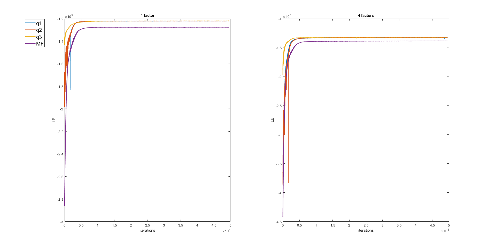
Figure 1: Plot of Lower Bound for variational approximations $q_{\lambda}^{I}$, $q_{\lambda}^{II}$, $q_{\lambda}^{III}$, and $q_{\lambda}^{MF}$ for simulated datasets.

Table 3: Simulated data for FSV models with $K=1$ and $4$ latent factors. Number of iterations $I$ (in thousands) and CPU time per iterations (in seconds) of the MCMC and variational methods. Average and standard deviation of the lower bound value over the last 5000 steps are also reported.

$K$	Methods	$\widehat{\mathcal{L}\left(\lambda\right)}$	$I$	CPU time	Total Time
1	PMCMC	NA	$30000$	$3.54$	$106200$
	$q_{\lambda}^{I}$	$-122130.41(27.45)$	$50000$	$0.11$	$5500$
	$q_{\lambda}^{II}$	$-122140.72(28.31)$	$50000$	$0.18$	$9000$
	$q_{\lambda}^{III}$	$-122020.77(23.99)$	$50000$	$0.14$	$7000$
	$q_{\lambda}^{MF}$	$-127707.31(37.13)$	$50000$	$0.03$	$1500$
4	PMCMC	NA	$30000$	$3.73$	$111900$
	$q_{\lambda}^{I}$	$-132501.73(48.89)$	$50000$	$0.13$	$6500$
	$q_{\lambda}^{II}$	$-132517.78(40.23)$	$50000$	$0.20$	$10000$
	$q_{\lambda}^{III}$	$-132116.92(32.02)$	$50000$	$0.17$	$8500$
	$q_{\lambda}^{MF}$	$-138454.19(51.74)$	$50000$	$0.04$	$2000$

Table 3 shows the average and standard deviation of the lower bound values for the variational methods for the FSV models with one and four factors. The estimated lower bound values can be used to select the best variational approximations. The $q_{\lambda}^{III}$ method has the highest estimated lower bound value, followed by $q_{\lambda}^{I}$, $q_{\lambda}^{II}$, and $q_{\lambda}^{MF}$. As expected, the $q_{\lambda}^{MF}$ has the lowest lower bound values. Surprisingly, the variational approximation $q_{\lambda}^{I}$ is better than $q_{\lambda}^{II}$ with larger number of variational parameters. The variational approximation $q_{\lambda}^{III}$ also has the smallest standard deviation of the lower bound. The variational methods are potentially much faster than reported as Figure 1 shows that all of the variational approximations already converge after $20000$ iterations.

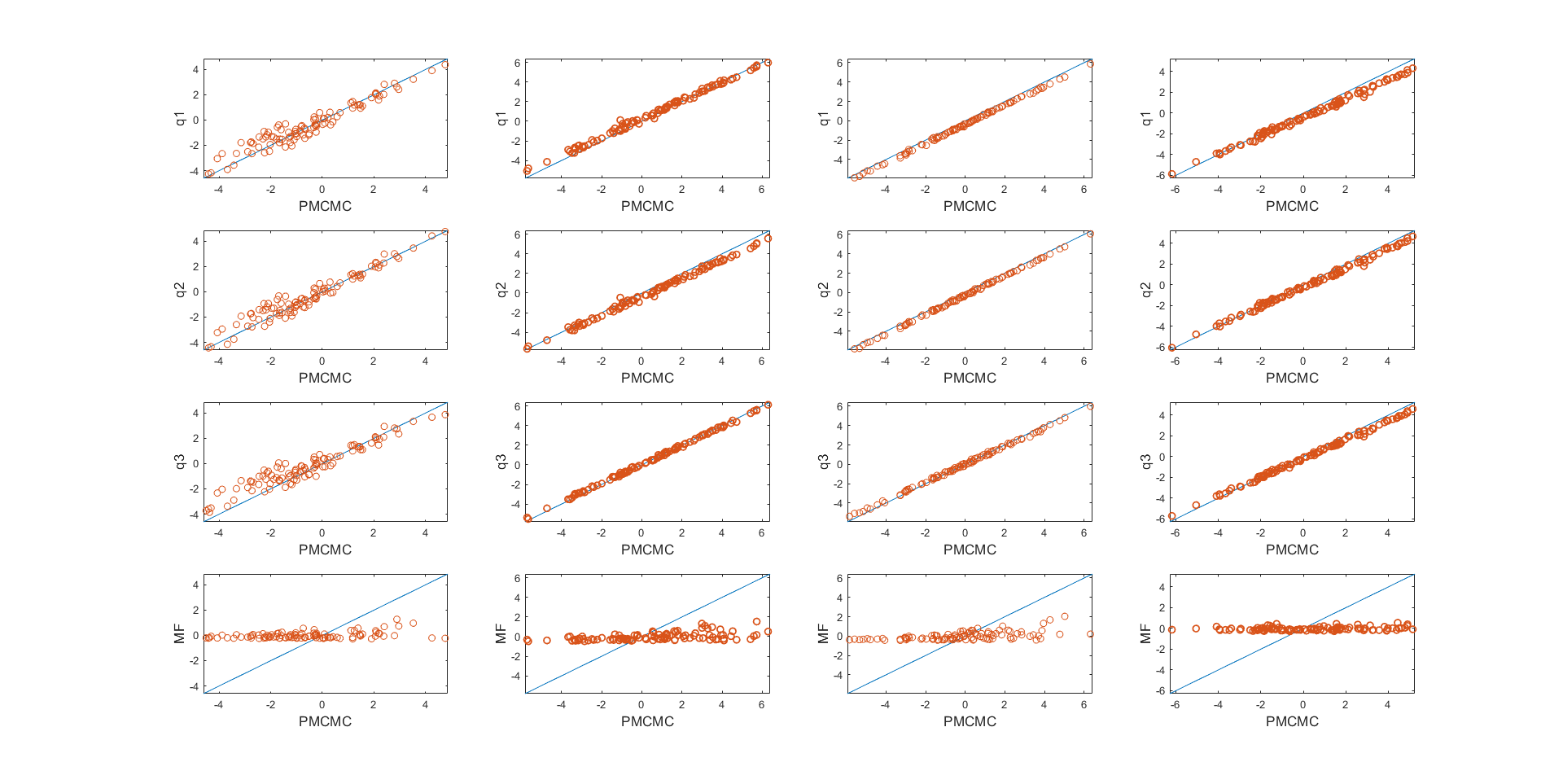
Figure 2: Simulated dataset. Scatter plots of the posterior means of the factors log-volatilities $h_{f,k,t}$, for $k=1,...,4$ and $t=10,20,...,1000$ estimated using particle MCMC on the x-axis and the variational approximation $q_{\lambda}^{I}$, $q_{\lambda}^{II}$, $q_{\lambda}^{III}$, and $q_{\lambda}^{MF}$, on the y-axis.

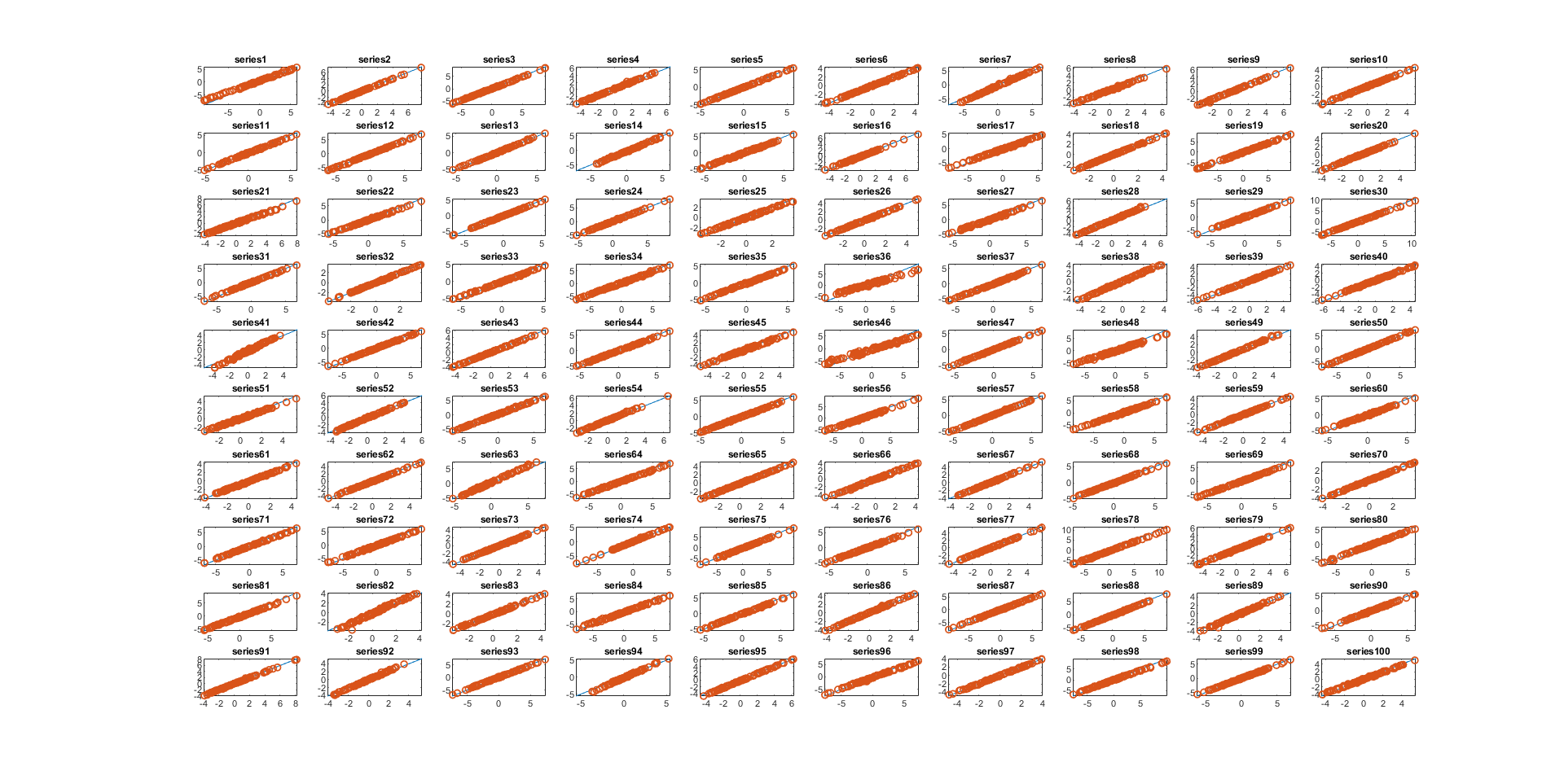
Figure 3: Simulated dataset. Scatter plots of the posterior means of the idiosyncratic log-volatility $h_{\epsilon,s,t}$, for $s=1,...,100$ and $t=10,20,...,1000$ estimated using particle MCMC on the x-axis and the variational approximation $q_{\lambda}^{III}$, on the y-axis.

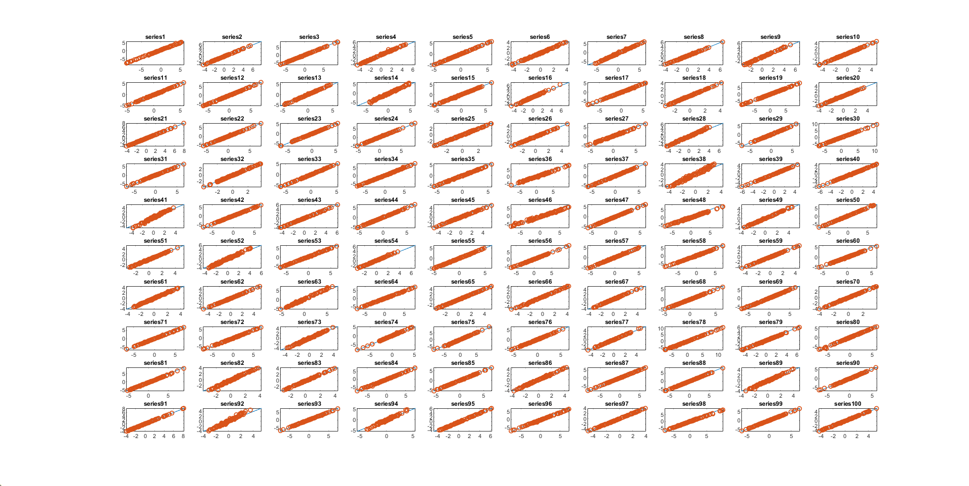
Figure S4: Simulated dataset. Scatter plots of the posterior means of the idiosyncratic log-volatilities $h_{\epsilon,s,t}$, for $s=1,...,100$ and $t=10,20,...,1000$ estimated using particle MCMC on the x-axis and the variational approximation $q_{\lambda}^{I}$ on the y-axis.

Figure S3 compares the posterior mean estimates of the factor log-volatilities $h_{f,k,t}$, for $k=1,...,4$, estimated using the different variational approximation methods and the particle MCMC method. The figure shows that all variational approximations give posterior mean estimates that are very close to each other and close to the particle MCMC estimates, except the mean-field variational approximation. Figure 3 and Figures S4, S5, and S6 (in Section S1 of the supplement) compare the variational posterior means of $q_{\lambda}^{III}$, $q_{\lambda}^{I}$, $q_{\lambda}^{II}$, and $q_{\lambda}^{MF}$ with the posterior means computed using the particle MCMC for all $S=100$ series. The figures show that the variational approximation $q_{\lambda}^{I}$, $q_{\lambda}^{II}$, and $q_{\lambda}^{III}$ estimate the posterior means accurately, but the mean-field variational approximation $q_{\lambda}^{MF}$ does not.

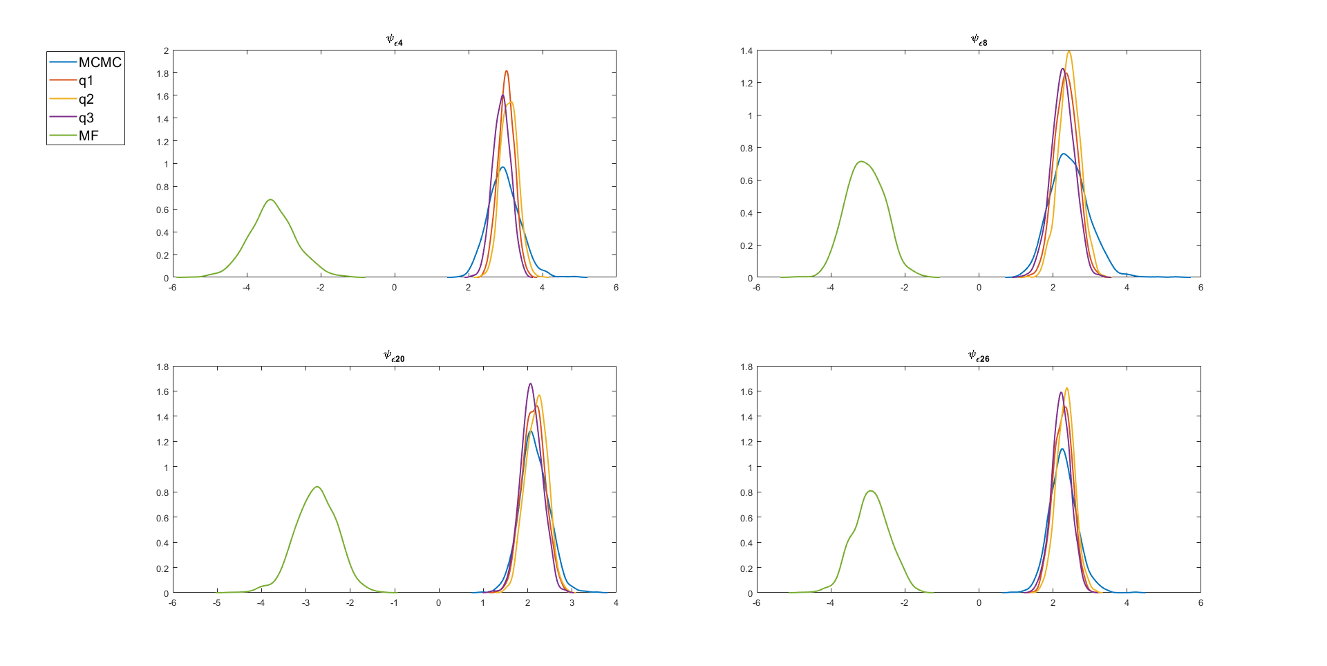
Figure 4: Simulated dataset. The marginal posterior density plots of the parameters $\left\{\psi_{\epsilon,4},\psi_{\epsilon,8},\psi_{\epsilon,20},\psi_{\epsilon,26}\right\}$ estimated using particle MCMC and VB with the variational approximations $q_{\lambda}^{I}$, and $q_{\lambda}^{II}$, $q_{\lambda}^{III}$, and $q_{\lambda}^{MF}$.

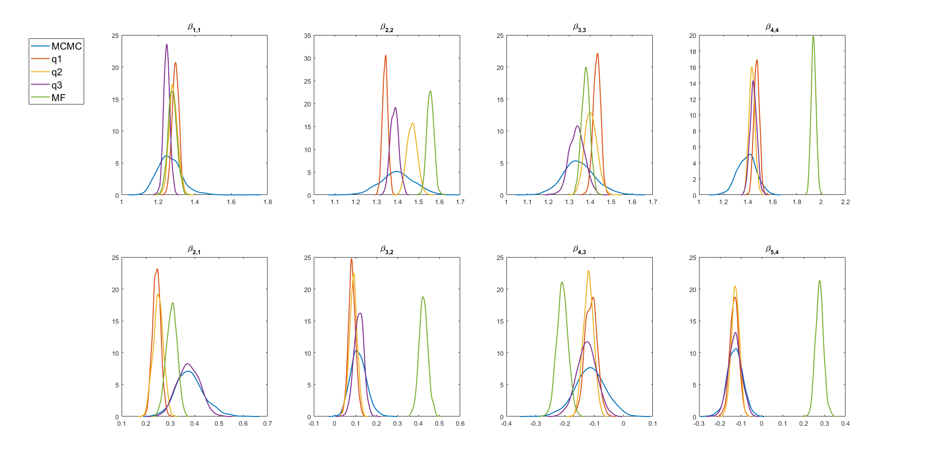
Figure 5: Simulated dataset. The marginal posterior density plots of some elements of the $\beta$ estimated using particle MCMC and VB with the variational approximations $q_{\lambda}^{I}$, and $q_{\lambda}^{II}$, $q_{\lambda}^{III}$, and $q_{\lambda}^{MF}$.

Figure 4 shows the marginal posterior densities of the parameters $\left\{\psi_{\epsilon,s}\right\}$ for $s=4,8,20,26$. All the variational approximations capture the posterior means quite well, except for the mean field variational approximation. There is a slight underestimation of the posterior variances of the $\psi$’s. Figure 5 shows the marginal posterior densities of some of the parameters in the factor loading matrix $\beta$. The variational approximation $q_{\lambda}^{III}$ captures the posterior means better than $q_{\lambda}^{I}$ and $q_{\lambda}^{II}$, but there is underestimation of the posterior variances of the $\beta$.

We now compare the predictive performance of the variational approximations with the (exact) particle MCMC method. The minimum variance portfolio implied by the $h$ step-ahead time-varying covariance matrix $\Sigma_{T+h}$, is considered which can be used to uniquely defines the optimal portfolio weights

$$w_{T+h}=\frac{\Sigma_{T+h}^{-1}\mathbb{1}}{\mathbb{1}^{\top}\Sigma_{T+h}^{-1}\mathbb{1}},$$

where $\mathbb{1}$ denotes an S-variate vector of ones (Bodnar et al.,, 2017). The optimal portfolio weights guarantee the lowest risk for a given expected portfolio return.

Figure 6 shows the multiple-step ahead predictive densities $\widehat{p}\left(y_{T+h}|y_{1:T}\right)$ of an optimally weighted combination of all series, for $h=1,...,10$ obtained using variational and PMCMC methods. The figure shows that all the variational predictive densities, except the mean-field variational approximation, are very close to the exact predictive densities obtained from the particle MCMC method with the $q_{\lambda}^{III}$ the closest to MCMC. Using the multivariate factor SV model, we can also obtain the predictive densities of the time-varying correlation between any two series. Given the time-varying covariance matrix at time $t$, the correlation matrix at time step $t$ is

$$\Gamma_{t}=\textrm{diag}\left(\Sigma_{t}\right)^{-\frac{1}{2}}\Sigma_{t}\textrm{diag}\left(\Sigma_{t}\right)^{-\frac{1}{2}}.$$

Figure 7 shows the multiple-step ahead predictive densities of the time-varying correlation between series 2 and 3 $\widehat{p}\left(\Gamma\left(y_{2,T+h},y_{3,T+h}\right)|y_{1:T}\right)$ for $h=1,...,10$. The figure shows that all the variational predictive, except the mean-field variational approximation, densities are very close to the exact predictive densities obtained from the PMCMC method. The estimates from the variational approximation $q_{\lambda}^{III}$ is the closest to MCMC. Both Figures 6 and 7 show that the variational predictive densities of our variational methods do not underestimate the predictive variances.

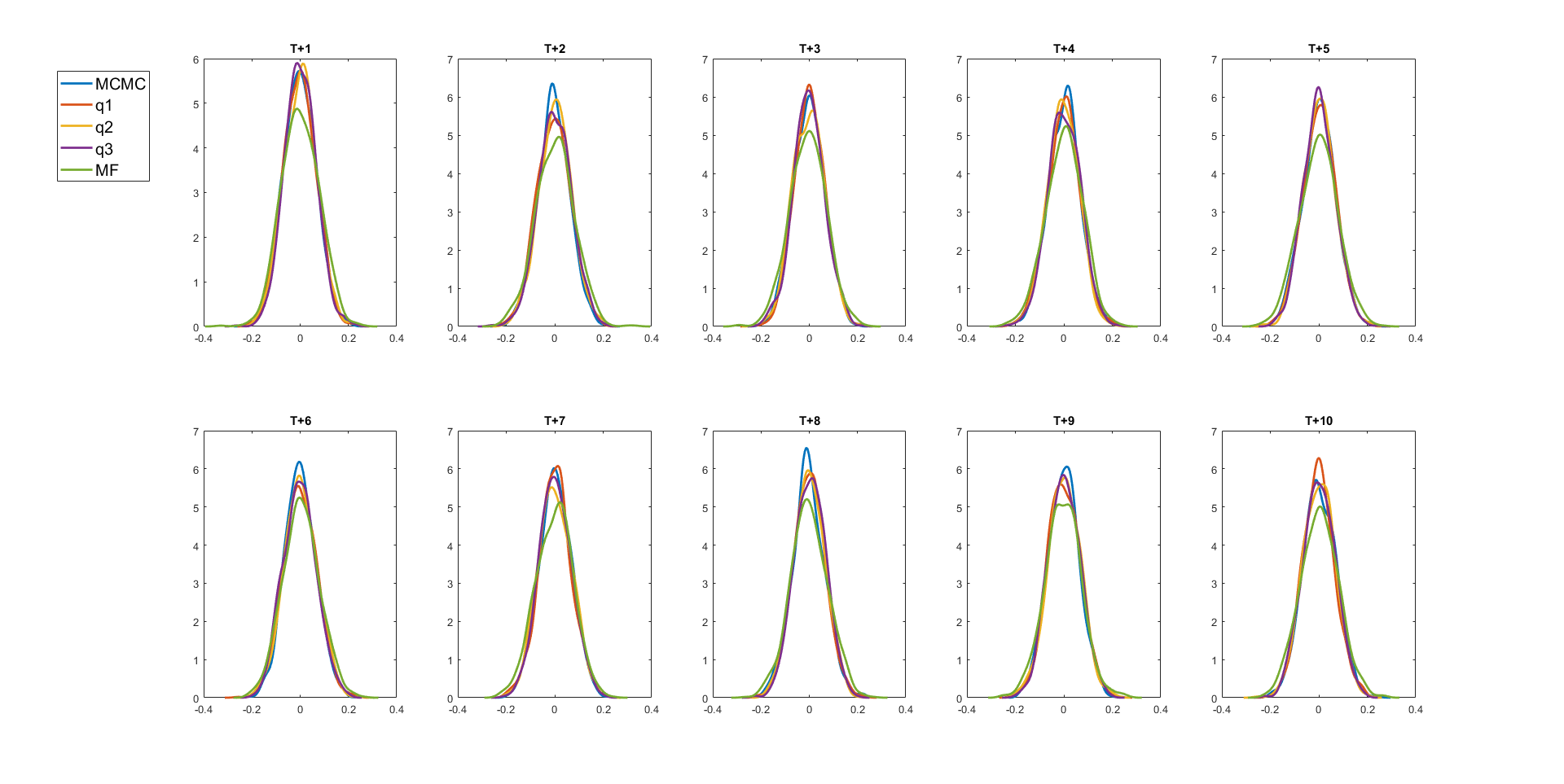
Figure 6: Simulated dataset. Plot of the predictive densities $\widehat{p}\left(y_{T+h}|y_{1:T}\right)$ of an optimally weighted series, for $h=1,...,10$, estimated using particle MCMC and the variational approximations $q_{\lambda}^{I}$, $q_{\lambda}^{II}$, $q_{\lambda}^{III}$, and $q_{\lambda}^{MF}$.

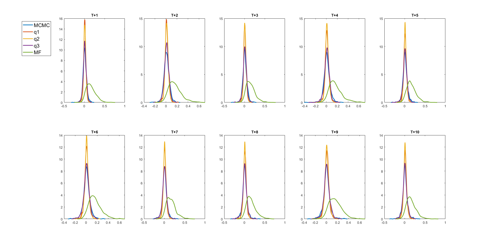
Figure 7: Simulated dataset. Plots of the predictive densities of the time-varying correlations $\widehat{p}\left(\Gamma\left(y_{2,T+h},y_{3,T+h}\right)|y_{1:T}\right),h=1,...,10$, between series 2 and 3 estimated using particle MCMC and the variational approximations $q_{\lambda}^{I}$, $q_{\lambda}^{II}$, $q_{\lambda}^{III}$, and $q_{\lambda}^{MF}$.

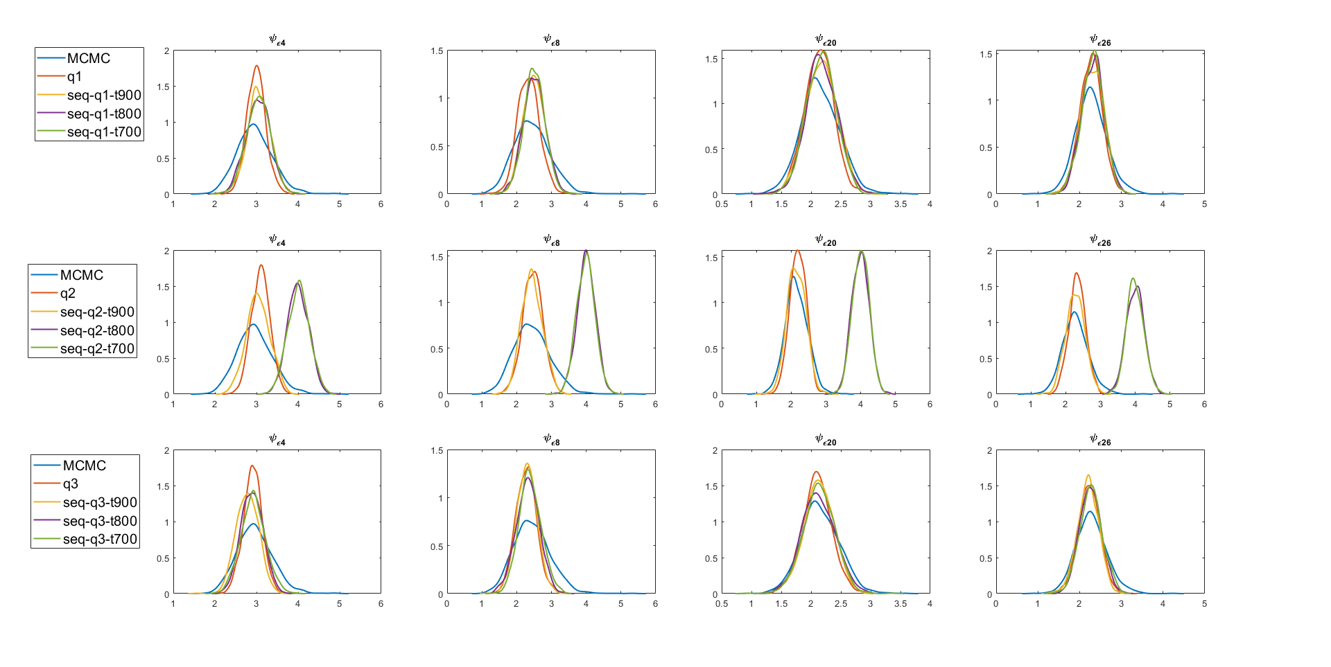
Figure S8: Simulated dataset. The marginal posterior density plots of the parameters $\left\{\psi_{\epsilon,4},\psi_{\epsilon,8},\psi_{\epsilon,20},\psi_{\epsilon,26}\right\}$ estimated using particle MCMC, batch VA, and sequential VA.

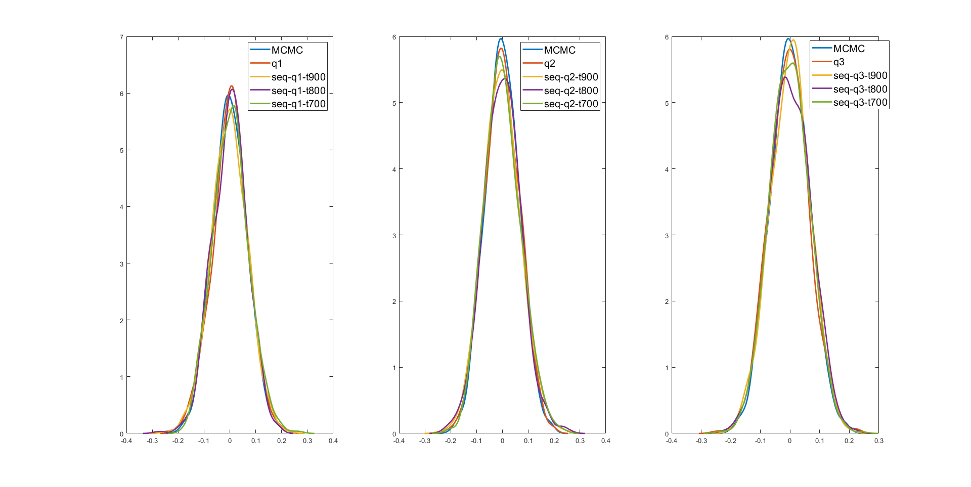
Figure S9: Simulated dataset. Plot of the predictive densities $\widehat{p}\left(y_{T+1}|y_{1:T}\right)$ of an optimally weighted series, estimated using particle MCMC, VA, and sequential VA.

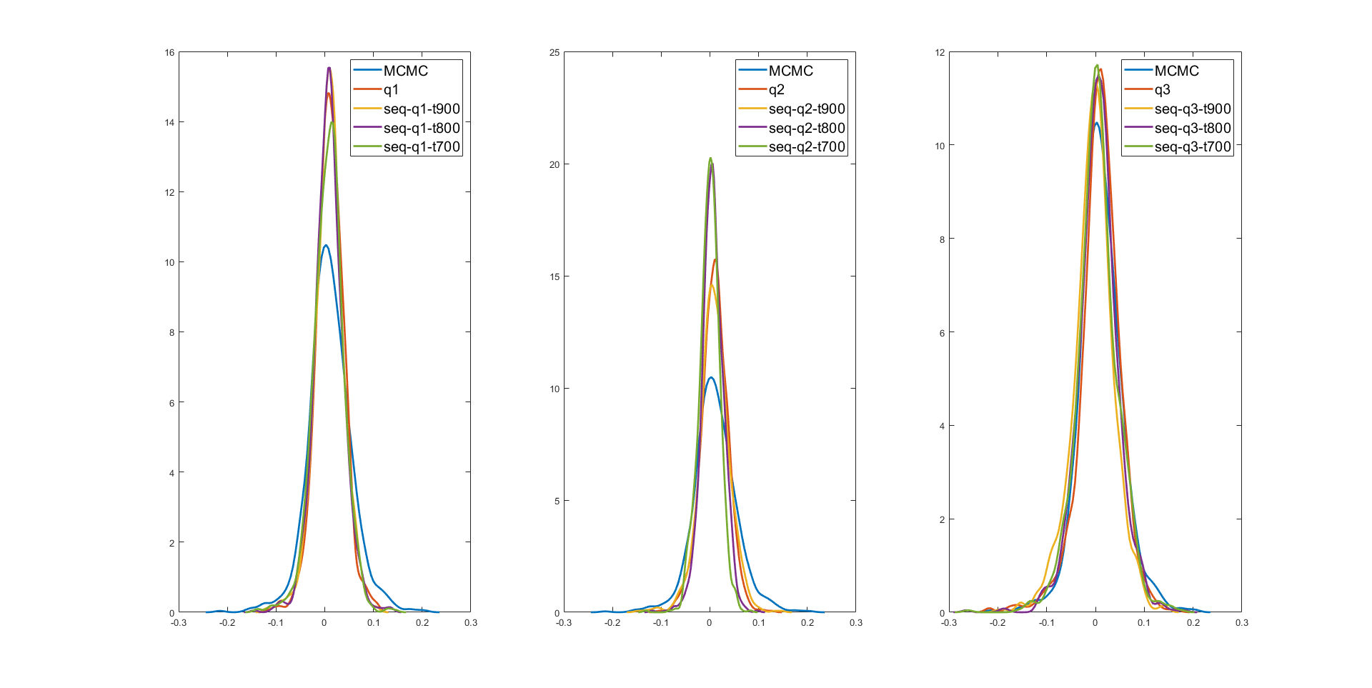
Figure S10: Simulated dataset. Plots of the predictive densities of the time-varying correlations $\widehat{p}\left(\Gamma\left(y_{2,T+1},y_{3,T+1}\right)|y_{1:T}\right)$, between series 2 and 3 estimated using particle MCMC, VA, and the sequential VA.

We now investigate the accuracy of the proposed sequential variational method described in Section 3.5 and consider the sequential versions of $q_{\lambda}^{I}$, $q_{\lambda}^{II}$, and $q_{\lambda}^{III}$. We do not consider the sequential version of the mean-field variational approximation because the batch version is less accurate than the other variational approximations. For each of the sequential VB methods, we consider three different starting points: $t=700$, $800$, and $900$. For example, the $t=700$ starting point means that the posterior of the parameters and latent variables is estimated as a batch for the first $t=700$ time points and then the posteriors are updated as new observations arrive up to $T=1000$; this method is denoted by $seq-q_{\lambda}-t700$. The updates for all sequential approaches are done after observing an additional $5$ time points for each series. Figure 8 shows the sequential lower bound for the variational approximation $seq-q_{\lambda}^{III}$ for the last 20 sequential updates with the starting point $t=900$. The figure shows that the sequential variational algorithm converges within $2000$ iterations or less for all sequential updates. Figure 9 and Figure S8 in Section S1 of the supplement show that the estimates from the sequential approaches $seq-q_{\lambda}^{I}$ and $seq-q_{\lambda}^{II}$ get worse with earlier starting points $t=700$ and $t=800$, but the estimates from $seq-q_{\lambda}^{III}$ are still close to $q_{\lambda}^{III}$ and MCMC for all cases. Similar observations can be made for the one-step-ahead prediction of the minimum variance portfolio in Figure S9 and one-step-ahead time-varying correlation between series 2 and 3 in Figure S10 in Section S1 of the supplement.

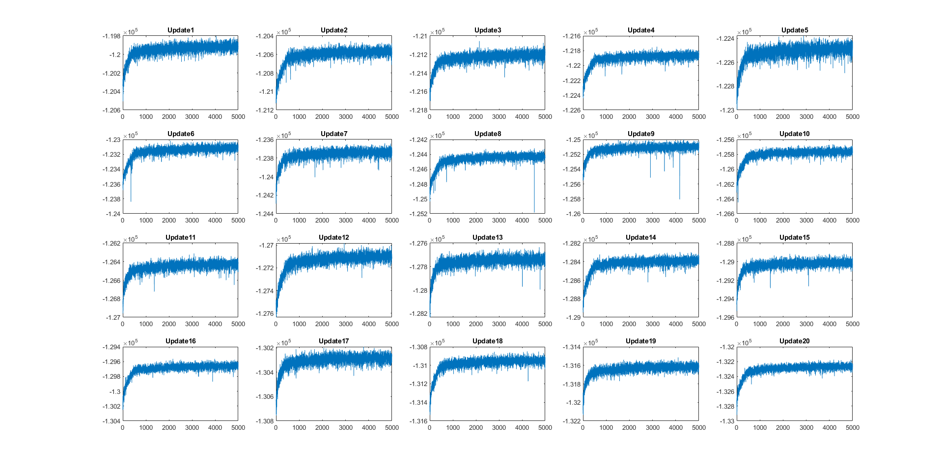
Figure 8: Simulated dataset. Plot of the sequential lower bound for the variational approximation $seq-q_{\lambda}^{III}$ for the last 20 sequential updates with starting point $t=900$.

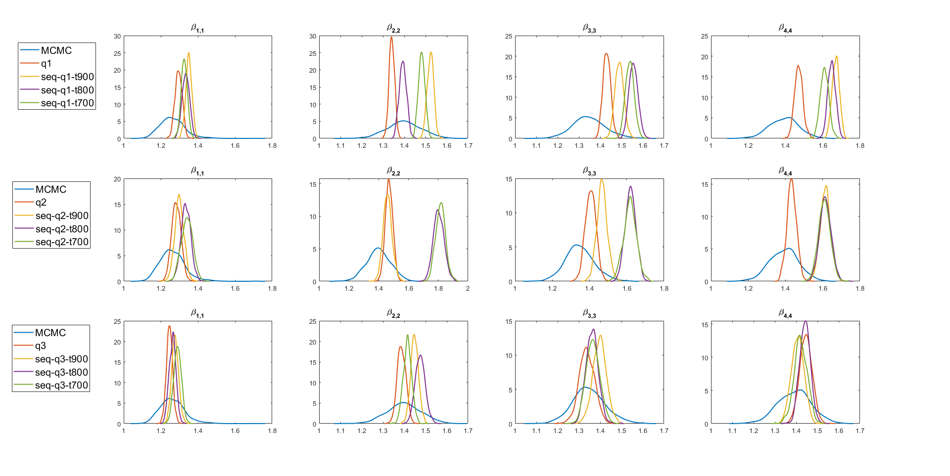
Figure 9: Simulated dataset. The marginal posterior density plots of some of the $\beta$ estimated using particle MCMC, VA, and sequential VA.

We conclude from the simulation study that the variational approximations are much faster than the exact MCMC approach. The variational approximations capture the posterior means of the parameters of the FSV model quite accurately, except for the mean field variational approximation, but there is some slight underestimation of the posterior variance for some of the parameters; The variational approximation $q_{\lambda}^{III}$ is the best. All the proposed variational approximations produce predictive densities for the returns and time-varying correlations between time series that are similar to the exact particle MCMC method with the $q_{\lambda}^{III}$ being the best; the variational approximation $q_{\lambda}^{I}$ is only slightly faster than $q_{\lambda}^{III}$ and much faster than $q_{\lambda}^{II}$, especially for long time series. The sequential variational approximation $seq-q_{\lambda}^{III}$ is also the most accurate of the sequential approximations. It is therefore important to take into account the posterior dependence between the latent factors and other latent states and parameters in the FSV model. It is important to take into account the dependence between parameters $\theta_{G,\epsilon,s}$ and the idiosyncratic log-volatilities $h_{\epsilon,s,1:T}$ for $s=1,...,S$ and the dependence between parameters $\theta_{G,f,k}$ and the factor log-volatilities $h_{f,k,1:T}$ for $k=1,...,K$. The dependence between $(\theta_{G,\epsilon,s},h_{\epsilon,s,1:T})$ and $(\theta_{G,\epsilon,j},h_{\epsilon,j,1:T})$ for $s\neq j$ and between $(\theta_{G,f,k},h_{f,k,1:T})$ and $(\theta_{G,f,j},h_{f,j,1:T})$ for $k\neq j$ can be possibly ignored. In terms of accuracy and CPU time, the variational approximation $q_{\lambda}^{III}$ and the sequential approximation $seq-q_{\lambda}^{III}$ are the best.

5.2 Application to US Stock Returns Data

Our methods are now applied to a panel of $S=90$ daily return of the Standard and Poor’s 100 stocks, from 9th of October 2009 to 30th September 2013 ($T=1000$ demeaned log returns in total). The data cover the following sectors: Consumer Discretionary, Consumer Staples, Energy, Financials, Health Care, Industrials, Information Technology, Materials, Telecommunication Services, and Utilities (see Appendix S3 for the individual stocks). The number of factors in the FSV model is selected using the lower bound and the cumulative log approximate predictive likelihood (CLAPL) values discussed in Section 4 using the variational approximation $q_{\lambda}^{III}$ as Section 5.1 shows that the $q_{\lambda}^{III}$ is the most accurate. The variational approximation is applied to the first $900$ time points and the CLAPL is computed for $t=901,...,1000$ time points. The number of Monte Carlo samples used to estimate the CLAPL at each time point is $M=10000$. Table 10 shows that the CLAPL values increase and then decrease. Similarly, the lower bound values increase significantly from $k=1$ factor to $k=4$ factors, and then flatten out. Therefore, further analysis in this section is based on four-factor FSV model.

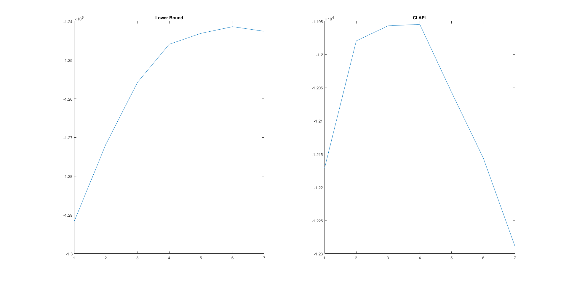
Figure 10: SP100 dataset. Plot of the average of the lower bound values for the last 5000 iterations (left) and the CLAPL values (right) for $k=1,...,7$ factors.

We study the performance of $q_{\lambda}^{I}$, $q_{\lambda}^{II}$, $q_{\lambda}^{III}$ and $q_{\lambda}^{MF}$ on the real data set. The accuracy of the variational approximations for the posterior and predictive densities are compared to the exact particle MCMC method with $N=100$ particles as in the simulation study in Section 5.1. The lower bound values (with standard deviations in brackets) are $-125307.64(47.15)$, $-125303.74(47.07)$, and $-124593.25(32.16)$ for the $q_{\lambda}^{I}$, $q_{\lambda}^{II}$, and $q_{\lambda}^{III}$, respectively. Clearly, $q_{\lambda}^{III}$ performs the best.

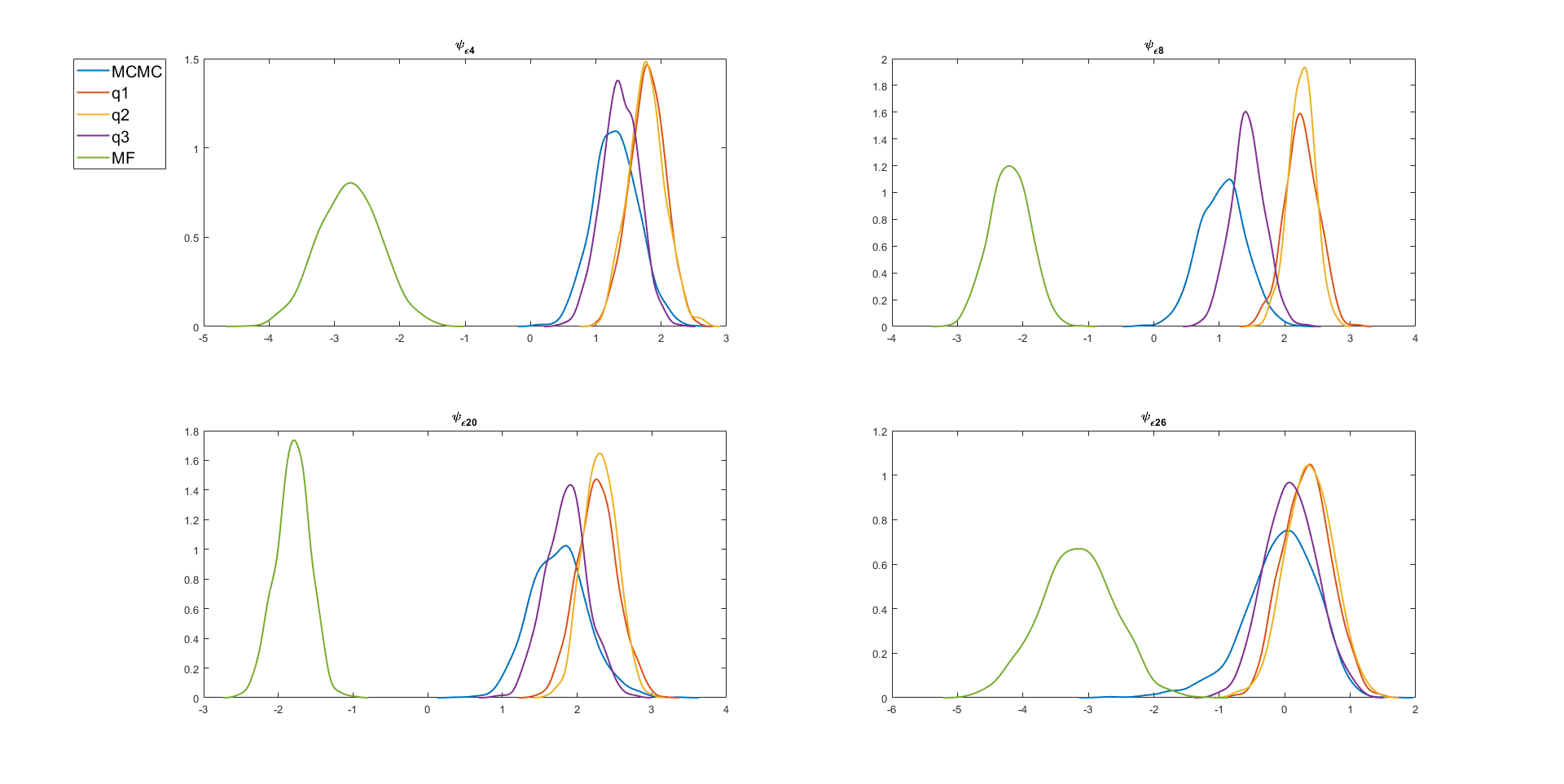
Figure 11: SP100 dataset. The marginal posterior density plots of the parameters $\left\{\psi_{\epsilon,4},\psi_{\epsilon,8},\psi_{\epsilon,20},\psi_{\epsilon,26}\right\}$ estimated using particle MCMC and VB with the variational approximations $q_{\lambda}^{I}$, $q_{\lambda}^{II}$, $q_{\lambda}^{III}$, and $q_{\lambda}^{MF}$.

Figure 12: SP100 dataset. Scatter plots of the posterior means of the latent factors $f_{k,t}$, for $k=1,...,4$ and $t=10,20,...,1000$ estimated using particle MCMC on the x-axis and the variational approximation $q_{\lambda}^{I}$, $q_{\lambda}^{II}$, $q_{\lambda}^{III}$, and $q_{\lambda}^{MF}$, on the y-axis.

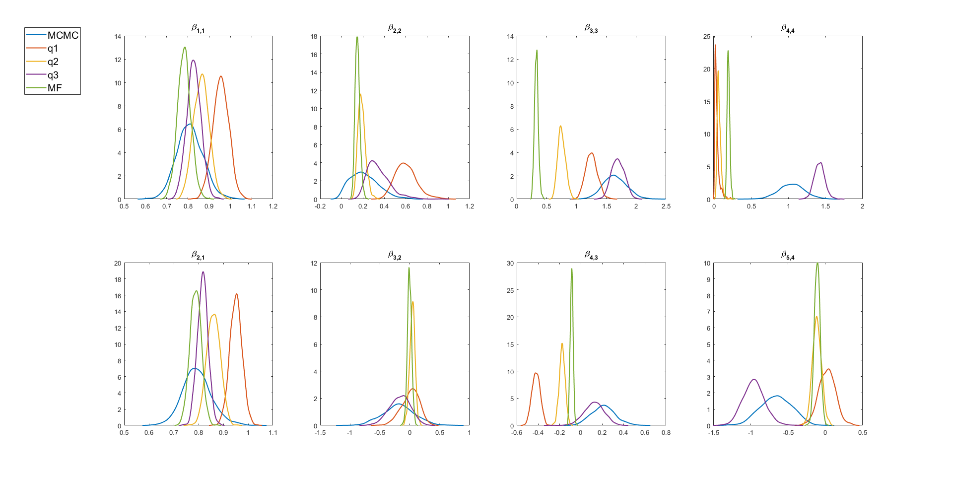
Figure S11: SP100 dataset. The marginal posterior density plots of some of the elements of $\beta$ estimated using particle MCMC, $q_{\lambda}^{I}$, $q_{\lambda}^{II}$, $q_{\lambda}^{III}$, and $q_{\lambda}^{MF}$.

Figure 11 shows the estimated marginal posterior densities of the parameters $\left\{\psi_{\epsilon,s}\right\}$ for $s=4,8,20,26$ using the different variational approximations and the exact MCMC method. The $q_{\lambda}^{III}$ approximation is able to capture the posterior means quite well compared to $q_{\lambda}^{I}$ and $q_{\lambda}^{II}$. The mean field variational approximation produces the wrong estimates. As in the simulation study, there is some underestimation of the posterior variance of the parameters in all the variational approximations. Similar conclusions can be made from Figures S11 and S12 in Appendix S2. Figure 12 shows the posterior mean estimates of the latent factors $f_{k,t}$, for $k=1,...,4$. All the variational approximations estimate posterior means of the first latent factor $f_{1,t}$ well, but the variational approximations $q_{\lambda}^{I}$, $q_{\lambda}^{II}$, and $q_{\lambda}^{MF}$ estimate the second to the fourth latent factors poorly. As expected, the variational approximation $q_{\lambda}^{III}$ estimates all the latent factors well. Similar conclusions can be made from Figures S13, S14, S15, and S16 in Appendix S2. This shows that the performances of the variational approximation, $q_{\lambda}^{III}$, still performs well when applied to real data.

The predictive performance of the variational approximations is now compared to that of the particle MCMC method using the minimum variance portfolio. Figure 13 shows the one-step ahead predictive density of the minimum variance portfolio estimated using the MCMC and the variational methods. The figure confirms that the mean-field variational approximation performs poorly. The estimates from $q_{\lambda}^{III}$ is the closest to the MCMC. Figure 14 plots the multiple-step ahead predictive densities of the time-varying correlation between Microsoft and AIG stock returns $\widehat{p}\left(\Gamma\left(y_{MSFT,T+h},y_{AIG,T+h}\right)|y_{1:T}\right)$ for $h=1,...,3$. The figure shows that all the variational predictive approximation densities, except the mean-field approximation, are very close to the exact predictive densities obtained from PMCMC. Again, the estimates from $q_{\lambda}^{III}$ is closest to MCMC. Both Figures 13 and 14 confirm that the variational predictive densities of our variational methods do not underestimate the predictive variances.

Figure 15 shows the mean estimates of one hundred step ahead predictive densities of the time-varying correlation between Microsoft and AIG, Amazon and Boeing, and JP Morgan and Morgan Stanley. The correlations between Microsoft and AIG, Amazon and Boeing, and JP Morgan and Morgan Stanley industries tend to increase over time. The mean-field variational approximation clearly does not capture this time-varying correlation obtained from MCMC and the other variational approximations.

Figure 13: SP100 dataset. Plot of the predictive densities $\widehat{p}\left(y_{T+1}|y_{1:T}\right)$ of the minimum variance portfolio, estimated using particle MCMC and the variational approximations $q_{\lambda}^{I}$, $q_{\lambda}^{II}$, $q_{\lambda}^{III}$, and $q_{\lambda}^{MF}$.

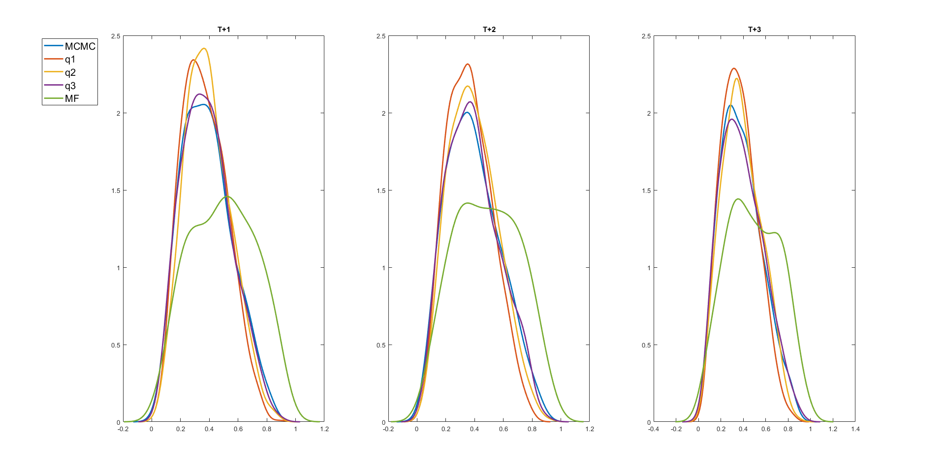
Figure 14: SP100 dataset. Plots of the predictive densities of the time-varying correlations $\widehat{p}\left(\Gamma\left(y_{MSFT,T+h},y_{AIG,T+h}\right)|y_{1:T}\right),h=1,2,3$, between Microsoft and AIG estimated using particle MCMC and the variational approximations $q_{\lambda}^{I}$, $q_{\lambda}^{II}$, $q_{\lambda}^{III}$, and $q_{\lambda}^{MF}$.

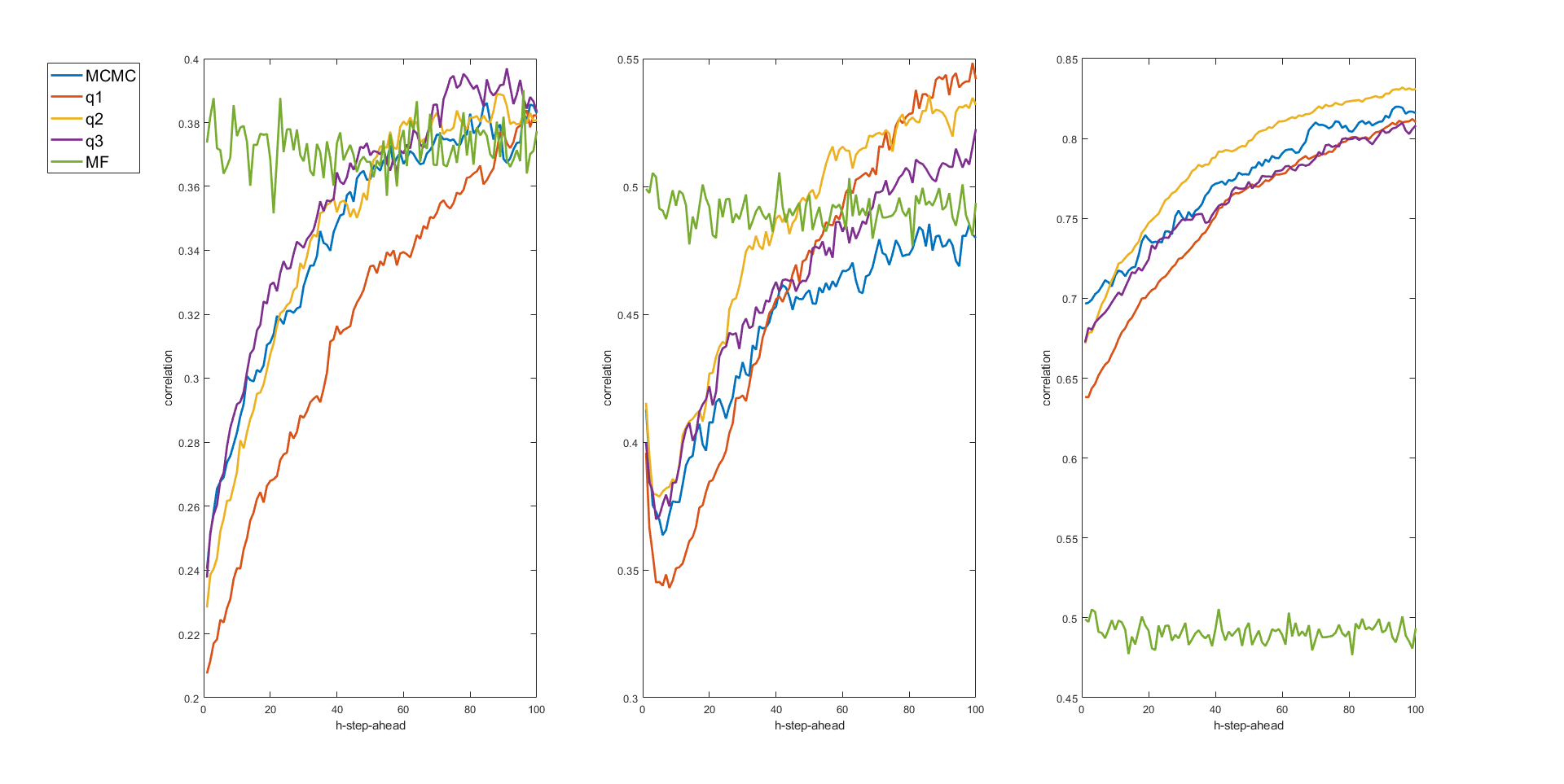
Figure 15: SP100 dataset. Plots of the mean estimates of one hundred step ahead predictive densities of the time-varying correlations between Microsoft and AIG (left), Amazon and Boeing (Middle), and JP Morgan and Morgan Stanley (Right) estimated using particle MCMC and the variational approximations $q_{\lambda}^{I}$, $q_{\lambda}^{II}$, $q_{\lambda}^{III}$, and $q_{\lambda}^{MF}$.

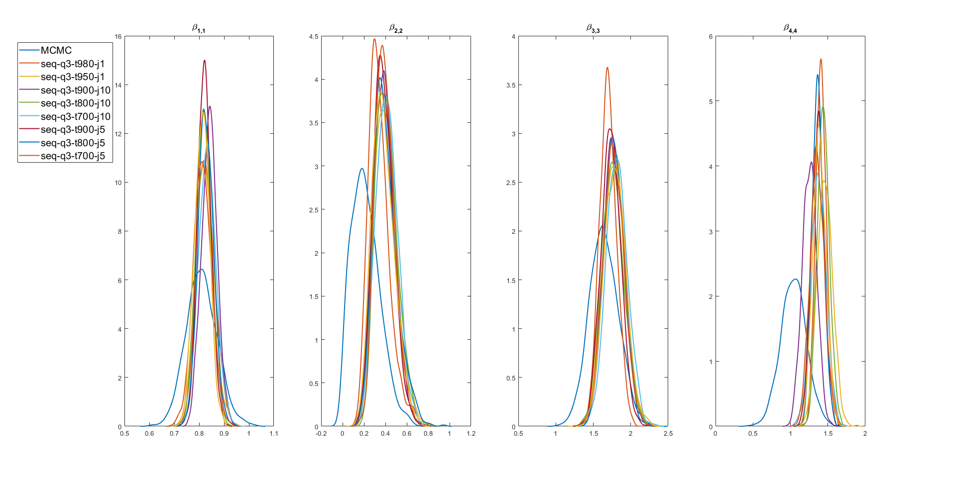
Figure S17: SP100 dataset. The marginal posterior density plots of some of the $\beta$ estimated using particle MCMC, $q_{\lambda}^{III}$ and $seq-q_{\lambda}^{III}$.

We now investigate the accuracy of the sequential variational method, in particular $seq-q_{\lambda}^{III}$ to the real data and compare it to standard $q_{\lambda}^{III}$ and particle MCMC. Different starting points and update frequencies are considered to evaluate the robustness of the sequential approach. The scenarios considered are: (1) starting points $t=950,980$ and updates after observing $j=1$ new observation until $T=1000$, (2) $t=700,800,900$ and $j=5$, and (3) $t=700,800,900$ and $j=10$. Figure 16 shows the estimated marginal posterior densities of the parameters $\left\{\psi_{\epsilon,s}\right\}$ for $s=1,4,20,26$ using the different batch variational approximations, sequential variational approximations, and particle MCMC. All the estimates from the different versions of the sequential approximations are very close to the standard variational approximation and the exact MCMC method. Similar conclusions can be made from Figure S17 in Appendix S2. This shows that the performance of $seq-q_{\lambda}^{III}$ does not deteriorate when applied to the real data and is robust to the starting points and update frequencies. Another important advantage of the sequential variational approximation $seq-q_{\lambda}^{III}$ is that it can provide sequential one-step ahead predictive densities of each stock return and any weighted portfolio as well as the time-varying correlation between industry stock returns; these are difficult to obtain using MCMC or particle MCMC approaches. For example, Figure 17 plots the sequential one-step ahead predictive densities of the minimum variance portfolio of the SP100 stock returns from 19th July 2013 to 30th September 2013.

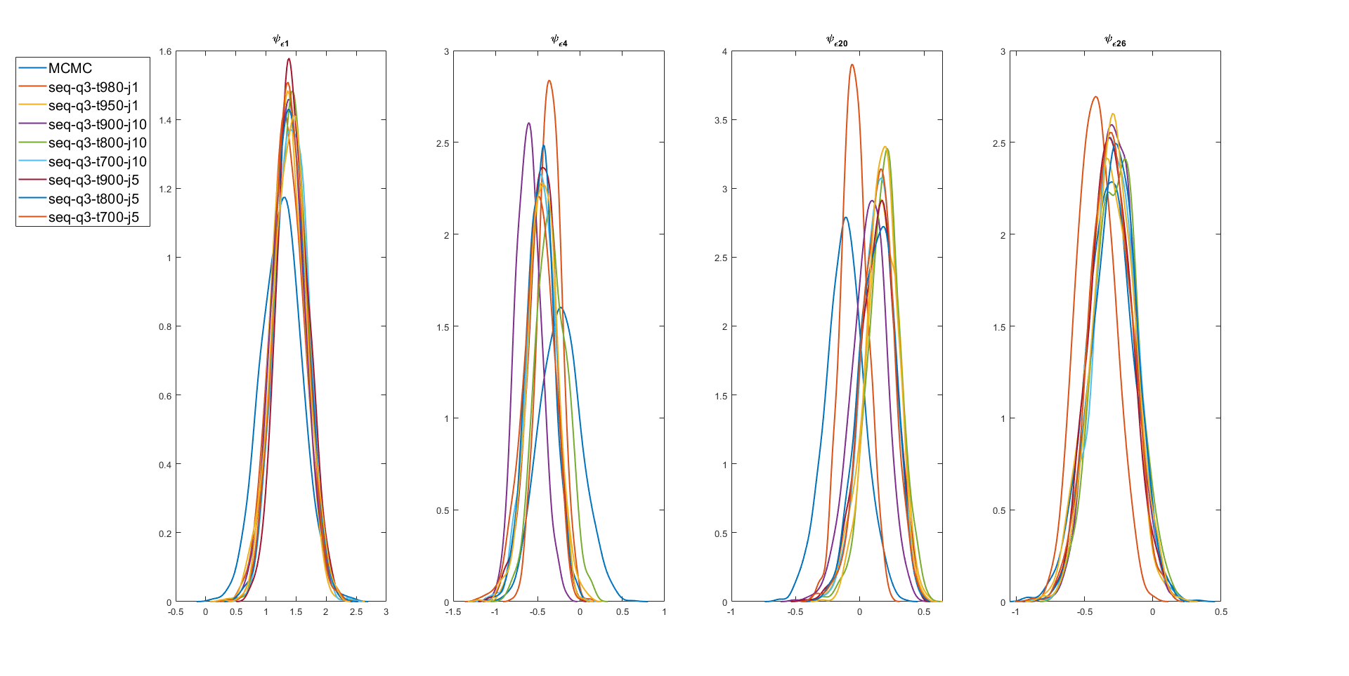
Figure 16: SP100 dataset. The marginal posterior density plots of the parameters $\left\{\psi_{\epsilon,4},\psi_{\epsilon,8},\psi_{\epsilon,20},\psi_{\epsilon,26}\right\}$ estimated using particle MCMC, $q_{\lambda}^{III}$, and $seq-q_{\lambda}^{III}$.

Figure 17: SP100 dataset. Plots of the sequential one-step-ahead predictive densities of the minimum variance portfolio estimated using the variational approximations $seq-q_{\lambda}^{III}$ from 19th July 2013 to 30th September 2013.

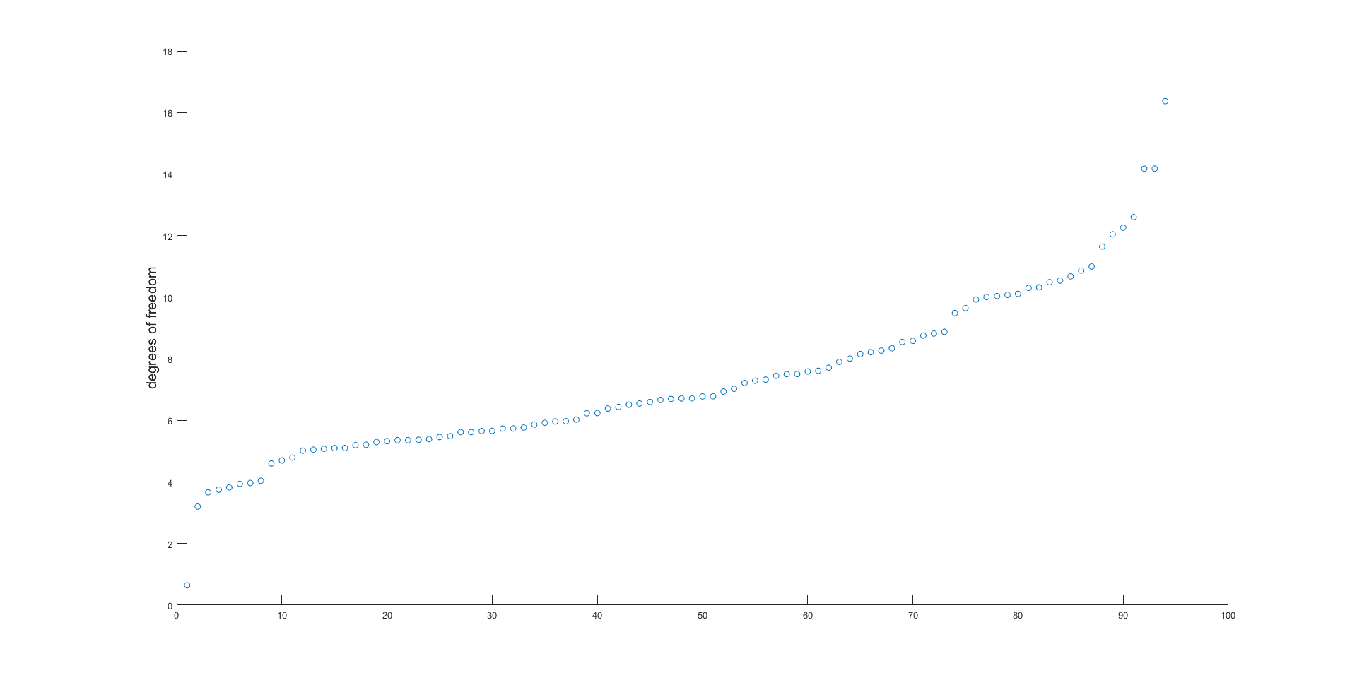
Figure S18: SP100 dataset. The posterior mean estimates of the degree of freedom parameters, $v_{f,k}$ for $k=1,...,4$ and $v_{\epsilon,s}$ for $s=1,...,90$ estimated using $q_{\lambda}^{III}$ (sorted in ascending order).

Finally, we compare the one-step-ahead predictive densities of some of the individual stock returns and the minimum variance portfolio from the FSV model with normal and t-distributions for the idiosyncratic and latent factor errors estimated using the variational approximations. Figure 18 shows the one-step-ahead predictive densities of Apple, JP Morgan, and Morgan Stanley industries as well as the minimum variance portfolio. It is clear that the predictive densities from the FSV model with t-distribution has some characteristics of financial stock returns, such as heavy tails, particularly in the left tails, and also sharper peaks in the middle of the distributions. Figure S18 in Appendix S2 plots the degree of freedom parameters $v_{f,k}$ for $k=1,...,K$ and $v_{\epsilon,s}$ for $s=1,...,S$.

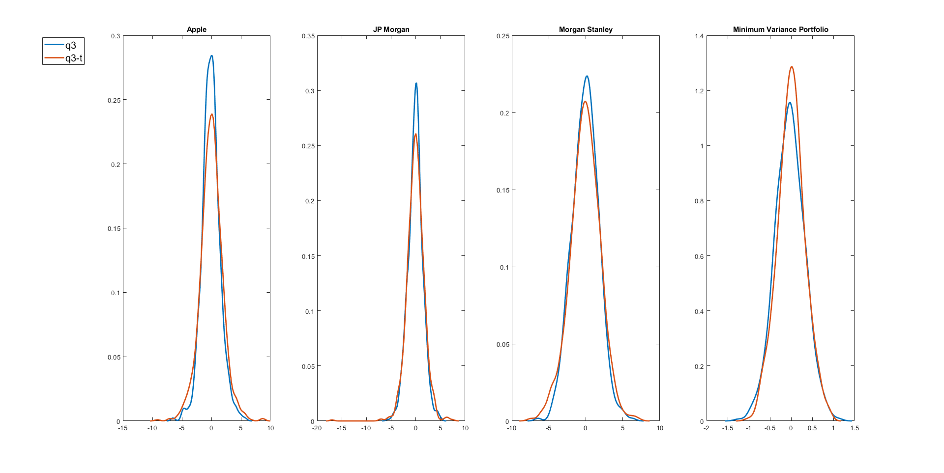
Figure 18: SP100 dataset. Plots of the one-step-ahead predictive densities of Apple, JP Morgan, Morgan Stanley, and the minimum variance portfolio estimated using variational approximation $q_{\lambda}^{III}$ for FSV models with normal and t distributions for the idiosyncratic errors.

6 Conclusions

This paper proposes fast and efficient variational methods for estimating posterior densities for the high dimensional FSV model in Section 2 with normal and t distributions for the idiosyncratic and latent factor errors. It also extends these batch methods to sequential variational updating that allows for one-step and multi-step ahead variational forecast distributions as new data arrives.

We show that the methods work well for both simulated and real data and are much faster than exact MCMC approaches. The data analyses suggest that a) Variational approaches are much faster than MCMC and particle MCMC approaches, especially for high dimensional time series. b) The variational approximations capture the posterior means of the parameters of the multivariate factor SV model quite accurately, except for the mean-field variational approximation; however, there is some slight underestimation in the posterior variances for some of the parameters. The variational approximation $q_{\lambda}^{III}$ is the most accurate for both the simulated and real datasets. It is therefore important to take into account the posterior dependence between the latent factors and other latent states and the parameters in the FSV model. The dependence between different idiosyncratic and factor log-volatilities can be ignored. c) The variational approximations $q_{\lambda}^{III}$ also produces the best one-step and multiple-step ahead predictive densities for the individual stock returns, the minimum variance portfolio, and the time-varying correlation between any pair of stock returns when compared to the exact particle MCMC method, without the problem of underestimating the prediction variance. d) The mean-field variational approximation appears to perform poorly in both batch and sequential modes. (e) The sequential approach $seq-q_{\lambda}^{III}$ is robust against the starting points and update frequencies and produces state and parameter estimates that are close to batch $q_{\lambda}^{III}$ and exact particle MCMC. It also accurately estimates the predictive densities of the individual stock returns, the minimum variance portfolio, and the time-varying correlation between any pair of stock returns.

The FSV model in the paper assumes that the factor loadings are static with uncorrelated latent factors and idiosyncratic errors. Therefore, it may require more factors to properly explain the comovement of multivariate time series than in more complex factor models which allow for time-varying factor loadings (Lopes and Carvalho,, 2007; Barigozzi and Hallin,, 2019), and correlated latent factors (Zhou et al.,, 2014) and idiosyncratic errors (Bai and Ng,, 2002). The FSV model in our article is still widely used in practice, for example Kastner, (2019), Kastner et al., (2017), and Li and Scharth, (2020). It is also straightforward to incorporate other distributions, such as t, skew normal, or skew-t distributions for the idiosyncratic errors and latent factors. Section S8 of the supplement discusses the FSV model with t-distribution for the idiosyncratic errors and latent factors. An immediate extension of our work would be to such more complex factor models.

Future work will consider developing variational approaches for other complex and high-dimensional time series models, such as the vector autoregressive model with stochastic volatility (VAR) of Chan et al., (2020) and multivariate financial time series model with recurrent neural network type architectures, e.g. the Long-Short term Memory model of Hochreiter and Schmidhuber, (1997).

Online Supplement for “Fast Variational Approximation for Multivariate Factor Stochastic Volatility Model”

S1 Additional Tables and Figures for the simulated dataset

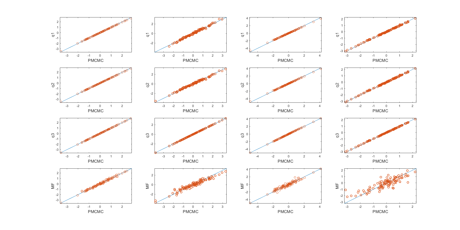
Figure S1: Simulated dataset. Scatter plots of the posterior means of the latent factors $f_{k,t}$, for $k=1,...,4$ and $t=10,20,...,1000$ estimated using particle MCMC on the x-axis and the variational approximation $q_{\lambda}^{I}$, $q_{\lambda}^{II}$, $q_{\lambda}^{III}$, and $q_{\lambda}^{MF}$, on the y-axis.

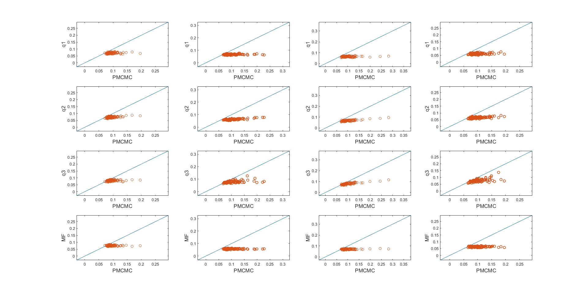
Figure S2: Simulated dataset. Scatter plots of the posterior standard deviation of the latent factors $f_{k,t}$, for $k=1,...,4$ and $t=10,20,...,1000$ estimated using particle MCMC on the x-axis and the variational approximation $q_{\lambda}^{I}$, $q_{\lambda}^{II}$, $q_{\lambda}^{III}$, and $q_{\lambda}^{MF}$, on the y-axis.

Figure S3: Simulated dataset. Scatter plots of the posterior means of the factors log-volatilities $h_{f,k,t}$, for $k=1,...,4$ and $t=10,20,...,1000$ estimated using particle MCMC on the x-axis and the variational approximation $q_{\lambda}^{I}$, $q_{\lambda}^{II}$, $q_{\lambda}^{III}$, and $q_{\lambda}^{MF}$, on the y-axis.

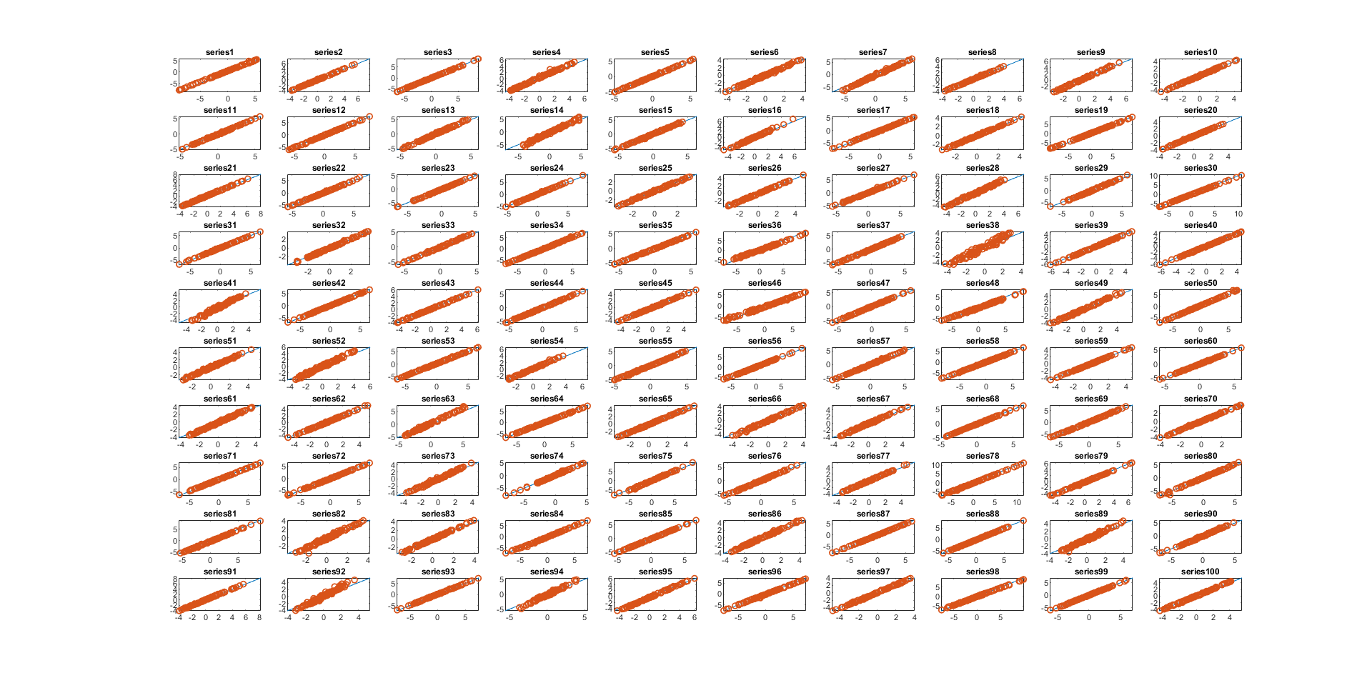
Figure S5: Simulated dataset. Scatter plots of the posterior means of the idiosyncratic log-volatilities $h_{\epsilon,s,t}$, for $s=1,...,100$ and $t=10,20,...,1000$ estimated using particle MCMC on the x-axis and the variational approximation $q_{\lambda}^{II}$ on the y-axis.

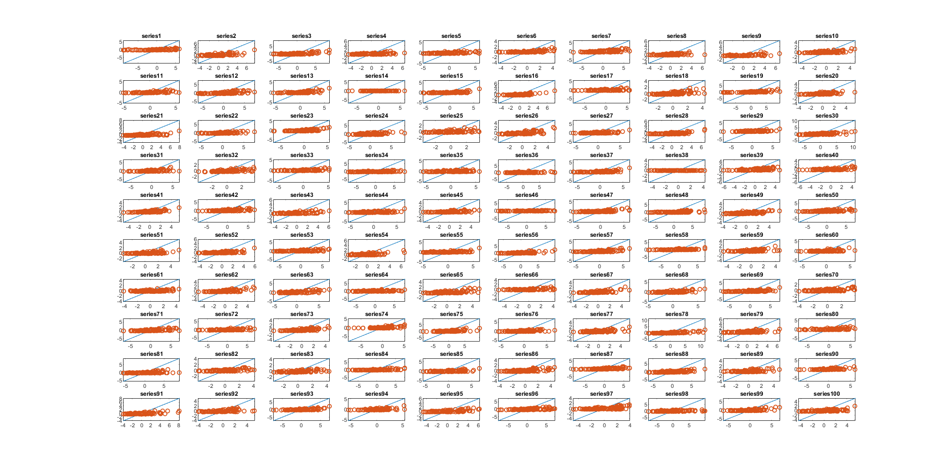
Figure S6: Simulated dataset. Scatter plots of the posterior means of the idiosyncratic log-volatilities $h_{\epsilon,s,t}$, for $s=1,...,100$ and $t=10,20,...,1000$ estimated using particle MCMC on the x-axis and the variational approximation $q_{\lambda}^{MF}$, on the y-axis.

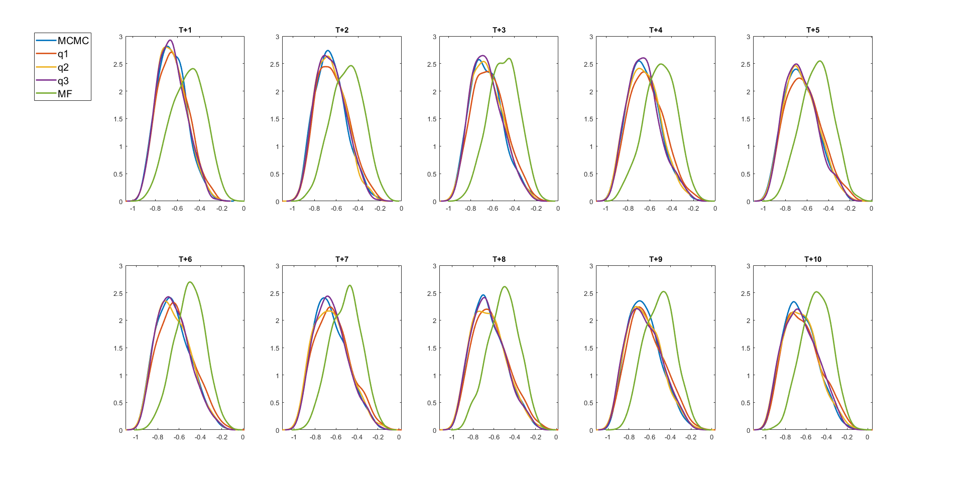
Figure S7: Simulated dataset. Plots of the predictive densities of the time-varying correlations $\widehat{p}\left(\Gamma\left(y_{2,T+h},y_{4,T+h}\right)|y_{1:T}\right),h=1,...,10$, between series 2 and 4 estimated using particle MCMC and the variational approximations $q_{\lambda}^{I}$, $q_{\lambda}^{II}$, $q_{\lambda}^{III}$, and $q_{\lambda}^{MF}$.

S2 Additional Tables and Figures for the SP100 dataset

Figure S12: SP100 dataset. The marginal posterior density plots of some of the 1st latent factors estimated using particle MCMC, $q_{\lambda}^{I}$, $q_{\lambda}^{II}$, $q_{\lambda}^{III}$ and $q_{\lambda}^{MF}$.

Figure S13: SP100 dataset. Scatter plots of the posterior means of the idiosyncratic log-volatilities $h_{\epsilon,s,t}$, for $s=1,...,90$ and $t=10,20,...,1000$ estimated using particle MCMC on the x-axis and the variational approximation $q_{\lambda}^{I}$ on the y-axis.

Figure S14: SP100 dataset. Scatter plots of the posterior means of the idiosyncratic log-volatilities $h_{\epsilon,s,t}$, for $s=1,...,90$ and $t=10,20,...,1000$ estimated using particle MCMC on the x-axis and the variational approximation $q_{\lambda}^{II}$ on the y-axis.

Figure S15: SP100 dataset. Scatter plots of the posterior means of the idiosyncratic log-volatilities $h_{\epsilon,s,t}$, for $s=1,...,90$ and $t=10,20,...,1000$ estimated using particle MCMC on the x-axis and the variational approximation $q_{\lambda}^{III}$, on the y-axis.

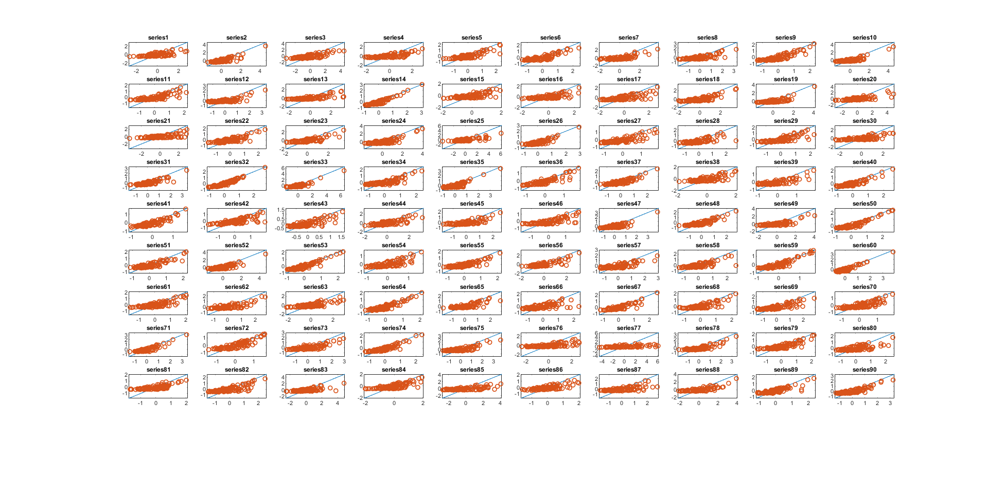
Figure S16: SP100 dataset. Scatter plots of the posterior means of the idiosyncratic log-volatilities $h_{\epsilon,k,t}$, for $s=1,...,90$ and $t=10,20,...,1000$ estimated using particle MCMC on the x-axis and the variational approximation $q_{\lambda}^{MF}$, on the y-axis.

S3 List of SP100 Stock Returns

Table S1: S&P100 constituents

Ticker	Name
AAPL	Apple Inc.	HPQ	Hewlett Packard Co.
ABT	Abbott Lab.	IBM	International Business Machines
AEP	American Electric Power Co.	INTC	Intel Corporation
AIG	American International Group Inc.	JNJ	Johnson and Johnson Inc.
ALL	Allstate Corp.	JPM	JP Morgan Chase & Co.
AMGN	Amgen Inc.	KO	The Coca-Cola Company
AMZN	Amazon.com	LLY	Eli Lilly and Company
APA	Apache Corp.	LMT	Lockheed-Martin
APC	Anadarko Petroleum Corp.	LOW	Lowe’s
AXP	American Express Inc.	MCD	McDonald’s Corp.
BA	Boeing Co.	MDT	Medtronic Inc.
BAC	Bank of America Corp.	MMM	3M Company
BAX	Baxter International Inc.	MO	Altria Group
BK	Bank of New York	MRK	Merck & Co.
BMY	Bristol-Myers Squibb	MS	Morgan Stanley
BRK.B	Berkshire Hathaway	MSFT	Microsoft
C	Citigroup Inc.	NKE	Nike
CAT	Caterpillar Inc.	NOV	National Oilwell Varco
CL	Colgate-Palmolive Co.	NSC	Norfolk Southern Corp.
CMCSA	Comcast Corp.	ORCL	Oracle Corporation
COF	Capital One Financial Corp.	OXY	Occidental Petroleum Corp.
COP	ConocoPhillips	PEP	Pepsico Inc.
COST	Costco	PFE	Pfizer Inc.
CSCO	Cisco Systems	PG	Procter and Gambel Co.
CVS	CVS Caremark	QCOM	Qualcomm Inc.
CVX	Chevron	RTN	Raytheon Co.
DD	DuPont	SBUX	Starbucks Corporation
DELL	Dell	SLB	Schlumberger
DIS	The Walt Disney Company	SO	Southern Company
DOW	Dow Chemical	SPG	Simon Property Group, Inc.
DVN	Devon Energy	T	AT&T Inc.
EBAY	eBay Inc.	TGT	Target Corp.
EMC	EMC Corporation	TWX	Time Warner Inc.
EMR	Emerson Electric Co.	TXN	Texas Instruments
EXC	Exelon	UNH	United Health Group Inc.
F	Ford Motor	UNP	Union Pacific Corp.
FCX	Freeport-McMoran	UPS	Uniter Parcel Service Inc.
FDX	FedEx	USB	US Bancorp
GD	General Dynamics	UTX	United Technologies Corp.
GE	General Electric Co.	VZ	Verizon Communication Inc.
GILD	Gilead Sciences	WAG	Walgreens
GS	Goldman Sachs	WFC	Wells Fargo
HAL	Haliburton	WMB	Williams Companies
HS	Home Depot	WMT	Wal-Mart
HON	HoneyWell	XOM	Exxon Mobil Corp.

S4 The factor loading matrix and the latent factors

This section discusses the parameterisation of the factor loading matrix $\beta$ and the latent factors $f_{t}$. The factor loading matrix $\beta$ is unidentified without further constraints (Geweke and Zhou,, 1996); we follow Geweke and Zhou, and assume that $\beta$ is lower triangular, i. e., $\beta_{s,k}=0$ for $k>s$. The restriction on the leading diagonal elements $\beta_{s,s}>0$ is also imposed. The main drawback of the lower triangular assumption on the factor loading matrix $\beta$ is that the resulting inference can depend on the order in which the components of $y_{t}$ are chosen (Chan et al.,, 2017). We follow Conti et al., (2014) and Kastner et al., (2017) to obtain an appropriate ordering of the returns for the real data. We run and post-process the factor loading estimates from the unrestricted sampler by choosing from column $1$, the stock $s$ with the largest value of $|\beta_{s,1}|$. We repeat this for columns $2$ to $7$. By an unrestricted sampler we mean that we do not restrict $\beta$ to be lower triangular.

S5 Particle MCMC for FSV Models

The key to making the estimation of the FSV model feasible is that given the latent factors $f_{1:T}$ and factor loading matrix $\beta$, the FSV model in Section 2 becomes $S$ independent univariate SV models for the idiosyncratic errors and $K$ independent univariate SV models for the latent factors. Conditional on the latent factors $f_{1:T}$ and factor loading matrix $\beta$, the $S$ univariate SV models with $\epsilon_{st}$ the $t$th observation on the $s$th SV model and the $K$ univariate SV models with $f_{kt}$ the $t$th observation on the $k$th univariate SV model can be estimated independently and in parallel. Gunawan et al., (2020) proposed a particle hybrid sampler for general state space models and they applied their method to estimate FSV model. They showed that the particle hybrid sampler is much more efficient than other PMCMC samplers available in the literature.

S6 Lower Bound and Reparameterisation Gradients for the Variational Approximation $q_{\lambda}^{III}\left(\theta,x_{1:T}\right)$

This section discusses the lower bound and reparameterisation gradients for the variational approximation $q_{\lambda}^{III}\left(\theta,x_{1:T}\right)$ for the FSV model. The set of parameters and latent variables in the FSV model is $\theta=\left(\left\{\kappa_{\epsilon,s},\alpha_{\epsilon,s},\psi_{\epsilon,s}\right\}_{s=1}^{S},\left\{\alpha_{f,k},\psi_{f,k}\right\}_{k=1}^{K},\beta\right)$ and $x_{1:T}=\left(\left\{h_{\epsilon,s,1:T}\right\}_{s=1}^{S},\left\{h_{f,k,1:T}\right\}_{k=1}^{K},\left\{f_{k,1:T}\right\}_{k=1}^{K}\right)$. We approximate the augmented posterior density $p\left(\theta,x_{1:T}|y\right)$ by

$$q_{\lambda}^{III}\left(\theta,x_{1:T}\right)=p\left(f_{1:T}|\theta,x_{1:T,-f_{1:T}},y\right)q_{\lambda}^{*}\left(\theta,x_{1:T,-f_{1:T}}|y\right),$$ (19)

where

$$q_{\lambda}^{*}\left(\theta,x_{1:T,-f_{1:T}}\right)=\prod_{s=1}^{S}q_{\lambda_{\epsilon,s}}^{TBN}\left(\theta_{\epsilon,s},h_{\epsilon,s,1:T}\right)\prod_{k=1}^{K}q_{\lambda_{f,k}}^{TBN}\left(\theta_{G,f,k},h_{f,k,1:T}\right)q_{\lambda_{\beta}}^{SRN}\left(\beta\right).$$ (20)

It is easy to generate the latent factors directly from their full conditional distribution $p\left(f_{1:T}|\theta,x_{1:T,-f_{1:T}},y\right)$ (see Section 3.4). After some simple algebra, the lower bound is

$$\mathcal{L}\left(\lambda\right)=E_{q}\left(\log p\left(y|f,h_{\epsilon},h_{f},\theta\right)+\log p\left(f|h_{\epsilon},h_{f},\theta\right)+\log p\left(h_{\epsilon},h_{f}|\theta\right)+\log p\left(\theta\right)-\right.\\ \left.\log p\left(f|\theta,h_{\epsilon},h_{f},y\right)-\log q_{\lambda}^{*}\left(\theta,h_{\epsilon},h_{f}|y\right)\right);$$ (21)

$h_{\epsilon}=\left\{h_{\epsilon,s,1:T}\right\}_{s=1}^{S}$, $h_{f}=\left\{h_{f,k,1:T}\right\}_{k=1}^{K}$, and $f=\left\{f_{k,1:T}\right\}_{k=1}^{K}$. From Bayes theorem,

$$p\left(f_{1:T}|\theta,x_{1:T,-f_{1:T}},y\right)=\frac{p\left(y|f,h_{\epsilon},h_{f},\theta\right)p\left(f|h_{\epsilon},h_{f},\theta\right)}{p\left(y|h_{\epsilon},h_{f},\theta\right)};$$

substituting this into Equation (21) gives

$$\mathcal{L}\left(\lambda\right)=E_{q}\left(\log p\left(y|h_{\epsilon},h_{f},\theta\right)+\log p\left(h_{\epsilon},h_{f}|\theta\right)+\log p\left(\theta\right)-\log q_{\lambda}^{*}\left(\theta,h_{\epsilon},h_{f}|y\right)\right).$$ (22)

A similar derivation to Loaiza-Maya et al., (2020) can be used to obtain the reparameterisation gradient. Let $\widetilde{\eta}=\left(\eta,f^{\top}\right)^{\top}$ with $\eta=\left(\left(\eta_{\theta_{G,\epsilon,s}}^{\top},\eta_{h_{1:T,\epsilon,s}}^{\top}\right)^{\top},\left(\eta_{\theta_{G,f,k}}^{\top},\eta_{h_{1:T,f,k}}^{\top}\right)^{\top},\eta_{\beta}^{\top}\right)$, have the product density $p_{\widetilde{\eta}}\left(\widetilde{\eta}\right)=p_{\eta}\left(\eta\right)p\left(f|u\left(\eta,\lambda\right),y\right)$, where $p_{\eta}\left(\eta\right)$ does not depend on the variational parameter $\lambda$, and

$$u\left(\eta,\lambda\right)=\left(u\left(\eta_{\beta},\lambda_{\beta}\right),\left\{u\left(\eta_{\theta_{G,\epsilon,s}},\eta_{h_{1:T,\epsilon,s}},\lambda_{\epsilon,s}\right)\right\}_{s=1}^{S},\left\{u\left(\eta_{\theta_{G,f,k}},\eta_{h_{1:T,f,k}},\lambda_{f,k}\right)\right\}_{k=1}^{K}\right),$$

so that $\left(\theta,x_{1:T}\right)=\left(u\left(\eta,\lambda\right),f\right)$. The reparameterisation gradient used to implement SGA is

$$\nabla_{\lambda}\mathcal{L}\left(\lambda\right)=E_{p_{\widetilde{\eta}}}\left(\nabla_{\lambda}u\left(\eta,\lambda\right)\left(\nabla_{\theta,x_{1:T,-f_{1:T}}}\log h\left(\theta,x_{1:T}\right)-\nabla_{\theta,x_{1:T,-f_{1:T}}}\log q_{\lambda}^{*}\left(\theta,h_{\epsilon},h_{f}|y\right)\right)\right),$$

where $h\left(\theta,x_{1:T}\right)=p\left(y|f,h_{\epsilon},h_{f},\theta\right)p\left(f|h_{\epsilon},h_{f},\theta\right)p\left(h_{\epsilon},h_{f}|\theta\right)p\left(\theta\right)$. The term $\nabla_{\theta,x_{1:T,-f_{1:T}}}\log p\left(f|\theta,h_{\epsilon},h_{f},y\right)$ is not needed, nor the derivatives with respect to the latent factors $f_{1:T}$, which simplifies the computation required for the reparameterisation gradient. We only need a single draw from the posterior distribution of the latent factors.

We now present the algorithm for the variational approximation $q_{\lambda}^{III}\left(\theta,x_{1:T}\right)$

Algorithm 2

Initialise all the variational parameters $\lambda$. At each iteration $j$, (1) Generate Monte Carlo samples for all the parameters and latent states from their variational distributions, (2) Compute the unbiased estimates of gradient of the lower bound with respect to each of the variational parameter and update the variational parameters using Stochastic Gradient methods.

STEP 1

• For $s=1:S$,

  • Generate Monte Carlo samples for $\theta_{G,\epsilon,s}$ and $h_{\epsilon,s,1:T}$ from the variational distribution $q_{\lambda_{\epsilon,s}}^{TBN}\left(\theta_{G,\epsilon,s},h_{\epsilon,s,1:T}\right)$

    1. Generate $\eta_{\theta_{G,\epsilon,s}}\sim N\left(0,I_{G_{\epsilon}}\right)$ and $\eta_{h_{1:T,\epsilon,s}}\sim N\left(0,I_{T}\right)$, where $G_{\epsilon}$ is the number of parameters of idiosyncratic log-volatilities

    2. Generate $\theta_{G,\epsilon,s}=\mu_{G,\epsilon,s}^{\left(j\right)}+\left(C_{G,\epsilon,s}^{\left(j\right)}\right)^{-\top}\eta_{\theta_{G,\epsilon,s}}$ and $h_{1:T,\epsilon,s}=\mu_{L,\epsilon,s}^{\left(j\right)}+\left(C_{L,\epsilon,s}^{\left(j\right)}\right)^{-\top}\eta_{x_{1:T,\epsilon,s}}$.

• For $k=1:K$,

  • Generate Monte Carlo samples for $\theta_{G,f,k}$ and $h_{f,k,1:T}$ from the variational distribution $q_{\lambda_{f,k}}^{TBN}\left(\theta_{G,f,k},h_{f,k,1:T}\right)$

    1. Generate $\eta_{\theta_{G,f,k}}\sim N\left(0,I_{G_{f}}\right)$ and $\eta_{h_{1:T,f,k}}\sim N\left(0,I_{T}\right)$, where $G_{f}$ is the number of parameters of factor log-volatilities

    2. Generate $\theta_{G,f,k}=\mu_{G,f,k}^{\left(j\right)}+\left(C_{G,f,k}^{\left(j\right)}\right)^{-\top}\eta_{\theta_{G,f,k}}$ and $h_{1:T,f,k}=\mu_{L,f,k}^{\left(j\right)}+\left(C_{L,f,k}^{\left(j\right)}\right)^{-\top}\eta_{x_{1:T,f,k}}$.

• Generate Monte Carlo samples for the factor loading $\beta$ from the variational distribution

  1. Generate $z_{\beta}\sim N\left(0,I_{p}\right)$ and $\eta_{\beta}\sim N\left(0,I_{R_{\beta}}\right)$ calculating $\xi_{\beta}=\mu_{\xi_{\beta}}^{\left(j\right)}+B^{\left(j\right)}_{\xi_{\beta}}z_{\beta}+d^{\left(j\right)}_{\xi_{\beta}}\circ\eta_{\beta}$, and $R_{\beta}$ is the total number of parameters in the factor loading matrix $\beta$.

  2. Generate $\beta_{i}=t_{\gamma_{\beta_{i}}}^{-1(j)}\left(\xi_{\beta_{i}}\right)$, for $i=1,...,R_{\beta}$.

• Generate Monte Carlo samples for the latent factors $f_{1:T}$ by sampling from its conditional distribution $p\left(f_{1:T}|\theta,x_{1:T,-f_{1:T}},y\right)$.

STEP 2

• For $s=1:S$, Update the variational parameters $\lambda_{\epsilon,s}$ of the variational distributions $q_{\lambda_{\epsilon,s}}^{TBN}\left(\theta_{\epsilon,s},h_{\epsilon,s,1:T}\right)$

  1. Construct unbiased estimates of gradients $\widehat{\nabla_{\lambda_{\epsilon,s}}\mathcal{L}\left(\lambda_{\epsilon,s}\right)}$.

  2. Set adaptive learning rates $a_{t,\epsilon,s}$ using ADAM method.

  3. Set $\lambda_{\epsilon,s}^{\left(j+1\right)}=\lambda_{\epsilon,s}^{\left(j\right)}+a_{j,\epsilon,s}\widehat{\nabla_{\lambda_{\epsilon,s}}\mathcal{L}\left(\lambda_{\epsilon,s}\right)}^{\left(j\right)}$,

     where $\lambda_{\epsilon,s}=\left\{\mu_{G,\epsilon,s}^{\top},v\left(C_{G,\epsilon,s}^{*}\right)^{\top},d_{\epsilon,s}^{\top},\textrm{vec}\left(D_{\epsilon,s}\right)^{\top},f_{\epsilon,s}^{*\top},\textrm{vec}\left(F_{\epsilon,s}\right)^{\top}\right\}^{\top}$ as defined in Section 3.2.

• For $k=1:K$,

  • Update the variational parameters $\lambda_{f,k}$ of the variational distributions $q_{\lambda_{f,k}}^{TBN}\left(\theta_{G,f,k},x_{f,k,1:T}\right)$

    1. Construct unbiased estimates of gradients $\widehat{\nabla_{\lambda_{f,k}}\mathcal{L}\left(\lambda_{f,k}\right)}$.

    2. Set adaptive learning rates $a_{j,f,k}$ using ADAM method.

    3. Set $\lambda_{f,k}^{\left(j+1\right)}=\lambda_{f,k}^{\left(j\right)}+a_{j,f,k}\widehat{\nabla_{\lambda_{f,k}}\mathcal{L}\left(\lambda_{f,k}\right)}^{\left(j\right)}$,

       where $\lambda_{f,k}=\left\{\mu_{G,f,k}^{\top},v\left(C_{G,f,k}^{*}\right)^{\top},d_{f,k}^{\top},\textrm{vec}\left(D_{f,k}\right)^{\top},f_{f,k}^{*\top},\textrm{vec}\left(F_{f,k}\right)^{\top}\right\}^{\top}$.

• Update the variational parameters $\lambda_{\beta}$ from the variational distribution $q_{\lambda_{\beta}}^{SRN}\left(\beta\right)$.

  1. Construct unbiased estimates of gradients $\widehat{\nabla_{\lambda_{\beta}}\mathcal{L}\left(\lambda_{\beta}\right)}$.

  2. Set adaptive learning rates $a_{t,\beta}$ using the ADAM method.

  3. Set $\lambda_{\beta}^{\left(j+1\right)}=\lambda_{\beta}^{\left(j\right)}+a_{j,\beta}\widehat{\nabla_{\lambda_{\beta}}\mathcal{L}\left(\lambda_{\beta}\right)}^{\left(j\right)}$, where $\lambda_{\beta}=\left(\gamma_{\beta_{1}}^{\top},...,\gamma_{\beta_{R_{\beta}}}^{\top},\mu_{\xi_{\beta}}^{\top},vech(B_{\xi_{\beta}})^{\top},d_{\xi_{\beta}}^{\top}\right)^{\top}$.

S7 Deriving the Gradients for the FSV Models

This section derives the gradients for the FSV models discussed in Section 2. The set of parameters and latent variables in the FSV model is given by $\theta=\left(\left\{\kappa_{\epsilon,s},\alpha_{\epsilon,s},\psi_{\epsilon,s}\right\}_{s=1}^{S},\left\{\alpha_{f,k},\psi_{f,k}\right\}_{k=1}^{K},\beta\right)$ and $x_{1:T}=\left(\left\{h_{\epsilon,s,1:T}\right\}_{s=1}^{S},\left\{h_{f,k,1:T}\right\}_{k=1}^{K},\left\{f_{k,1:T}\right\}_{k=1}^{K}\right)$. The required gradients are:

• For $s=1,...,S$,

  $$\nabla_{\alpha_{\epsilon,s}}\log p\left(y,\theta,x_{1:T}\right)=\frac{1}{2}\sum_{t=1}^{T}\left(h_{\epsilon,s,t}\left(y_{t}-\beta f_{t}\right)^{2}\exp\left(-\tau_{\epsilon,s}h_{\epsilon,s,t}-\kappa_{\epsilon,s}\right)-h_{\epsilon,s,t}\right)\left(1-\exp\left(-\tau_{\epsilon,s}\right)\right)\\ -\frac{2\tau_{\epsilon,s}}{\left(1+\tau_{\epsilon,s}^{2}\right)}\frac{\exp\left(\alpha_{\epsilon,s}\right)}{1+\exp\left(\alpha_{\epsilon,s}\right)}+1-\frac{\exp\left(\alpha_{\epsilon,s}\right)}{1+\exp\left(\alpha_{\epsilon,s}\right)};$$

$$\nabla_{\kappa_{\epsilon,s}}\log p\left(y,\theta,x_{1:T}\right)=\frac{1}{2}\left(\sum_{t=1}^{T}\left(y_{t}-\beta f_{t}\right)^{2}\exp\left(-\tau_{\epsilon,s}h_{\epsilon,s,t}-\kappa_{\epsilon,s}\right)-T\right)-\kappa_{\epsilon,s}/\sigma_{\kappa}^{2};$$

$$\nabla_{\psi_{\epsilon,s}}\log p\left(y,\theta,x_{1:T}\right)=\left(\sum_{t=2}^{T}\left(h_{\epsilon,s,t}-\phi_{\epsilon,s}h_{\epsilon,s,t-1}\right)h_{\epsilon,s,t-1}+h_{\epsilon,s,1}^{2}\phi_{\epsilon,s}-\frac{\phi_{\epsilon,s}}{1-\phi_{\epsilon,s}^{2}}\right)\left(\phi_{\epsilon,s}\left(1-\phi_{\epsilon,s}\right)\right)+\\ \left(\frac{\left(a_{0}-1\right)}{\left(1+\phi_{\epsilon,s}\right)}-\frac{\left(b_{0}-1\right)}{\left(1-\phi_{\epsilon,s}\right)}\right)\frac{\exp\left(\psi_{\epsilon,s}\right)}{\left(1+\exp\left(\psi_{\epsilon,s}\right)\right)^{2}}+\frac{\left(1-\exp\left(\psi_{\epsilon,s}\right)\right)}{\left(1+\exp\left(\psi_{\epsilon,s}\right)\right)};$$

$$\nabla_{h_{\epsilon,s,1}}\log p\left(y,\theta,x_{1:T}\right)=\frac{\tau_{\epsilon,s}}{2}\left(\left(y_{1}-\beta f_{1}\right)^{2}\exp\left(-\tau_{\epsilon,s}h_{\epsilon,s,1}-\kappa_{\epsilon,s}\right)-1\right)+\\ \phi_{\epsilon,s}\left(h_{\epsilon,s,2}-\phi_{\epsilon,s}h_{\epsilon,s,1}\right)-h_{\epsilon,s,1}\left(1-\phi_{\epsilon,s}^{2}\right);$$

$$\nabla_{h_{\epsilon,s,T}}\log p\left(y,\theta,x_{1:T}\right)=\frac{\tau_{\epsilon,s}}{2}\left(\left(y_{T}-\beta f_{T}\right)^{2}\exp\left(-\tau_{\epsilon,s}h_{\epsilon,s,T}-\kappa_{\epsilon,s}\right)-1\right)-\\ \left(h_{\epsilon,s,T}-\phi_{\epsilon,s}h_{\epsilon,s,T-1}\right);$$

$$\nabla_{h_{\epsilon,s,t}}\log p\left(y,\theta,x_{1:T}\right)=\frac{\tau_{\epsilon,s}}{2}\left(\left(y_{t}-\beta f_{t}\right)^{2}\exp\left(-\tau_{\epsilon,s}h_{\epsilon,s,t}-\kappa_{\epsilon,s}\right)-1\right)+\\ \phi_{\epsilon,s}\left(h_{\epsilon,s,t+1}-\phi_{\epsilon,s}h_{\epsilon,s,t}\right)-\left(h_{\epsilon,s,t}-\phi_{\epsilon,s}h_{\epsilon,s,t-1}\right)\;\textrm{for}\;t=2,...,T-1;$$

• For $k=1,...,K,$

  $$\nabla_{\alpha_{f,k}}\log p\left(y,\theta,x_{1:T}\right)=\frac{1}{2}\sum_{t=1}^{T}\left(h_{f,k,t}\left(f_{k,t}\right)^{2}\exp\left(-\tau_{f,k}h_{f,k,t}\right)-h_{f,k,t}\right)\left(1-\exp\left(-\tau_{f,k}\right)\right)\\ -\frac{2\tau_{f,k}}{\left(1+\tau_{f,k}^{2}\right)}\frac{\exp\left(\alpha_{f,k}\right)}{1+\exp\left(\alpha_{f,k}\right)}+1-\frac{\exp\left(\alpha_{f,k}\right)}{1+\exp\left(\alpha_{f,k}\right)};$$

$$\nabla_{\psi_{f,k}}\log p\left(y,\theta,x_{1:T}\right)=\left(\sum_{t=2}^{T}\left(h_{f,k,t}-\phi_{f,k}h_{f,k,t-1}\right)h_{f,k,t-1}+h_{f,k,1}^{2}\phi_{f,k}-\frac{\phi_{f,k}}{1-\phi_{f,k}^{2}}\right)\left(\phi_{f,k}\left(1-\phi_{f,k}\right)\right)+\\ \left(\frac{\left(a_{0}-1\right)}{\left(1+\phi_{f,k}\right)}-\frac{\left(b_{0}-1\right)}{\left(1-\phi_{f,k}\right)}\right)\frac{\exp\left(\psi_{f,k}\right)}{\left(1+\exp\left(\psi_{f,k}\right)\right)^{2}}+\frac{\left(1-\exp\left(\psi_{f,k}\right)\right)}{\left(1+\exp\left(\psi_{f,k}\right)\right)};$$

$$\nabla_{h_{f,k,1}}\log p\left(y,\theta,x_{1:T}\right)=\frac{\tau_{f,k}}{2}\left(\left(f_{k,1}\right)^{2}\exp\left(-\tau_{f,k}h_{f,k,1}\right)-1\right)+\\ \phi_{f,k}\left(h_{f,k,2}-\phi_{f,k}h_{f,k,1}\right)-h_{f,k,1}\left(1-\phi_{f,k}^{2}\right);$$

$$\nabla_{h_{f,k,T}}\log p\left(y,\theta,x_{1:T}\right)=\frac{\tau_{f,k}}{2}\left(\left(f_{k,T}\right)^{2}\exp\left(-\tau_{f,k}h_{f,k,T}\right)-1\right)-\\ \left(h_{f,k,T}-\phi_{f,k}h_{f,k,T-1}\right);$$

$$\nabla_{h_{f,k,t}}\log p\left(y,\theta,x_{1:T}\right)=\frac{\tau_{f,k}}{2}\left(\left(f_{k,t}\right)^{2}\exp\left(-\tau_{f,k}h_{f,k,t}\right)-1\right)+\\ \phi_{f,k}\left(h_{f,k,t+1}-\phi_{f,k}h_{f,k,t}\right)-\left(h_{f,k,t}-\phi_{f,k}h_{f,k,t-1}\right)\;\textrm{for}\;t=2,...,T-1.$$

• The gradients with respect to the latent factors $f_{t}$, for $t=1,...,T$,

  $$\nabla_{f_{t}}\log p\left(y,\theta,x_{1:T}\right)=\left(y_{t}-\beta f_{t}\right)^{{}^{\prime}}V_{t}^{-1}\beta-f_{t}^{{}^{\prime}}D_{t}^{-1};$$

  where

  $$V_{t}=\textrm{diag}\left(\exp\left(\tau_{\epsilon,1}h_{\epsilon,1,t}+\kappa_{\epsilon,1}\right),...,\exp\left(\tau_{\epsilon,S}h_{\epsilon,S,t}+\kappa_{\epsilon,S}\right)\right);$$

  $$D_{t}=\textrm{diag}\left(\exp\left(\tau_{f,1}h_{f,1,t}\right),...,\exp\left(\tau_{f,K}h_{f,K,t}+\kappa_{f,K}\right)\right).$$

• The gradients with respect to the factor loading $\beta_{s,.}=\left(\beta_{s,1},...,\beta_{s,k_{s}}\right)^{{}^{\prime}}$ for $s=1,...,S$:

  $$\nabla_{\beta_{s,.}}\log p\left(y,\theta,x_{1:T}\right)=\left(y_{s,1:T}-F_{s}\beta_{s,.}\right)^{{}^{\prime}}\widetilde{V}_{s}^{-1}F_{s}-\nabla_{\beta_{s,.}}\log p\left(\beta_{s,.}\right),$$

  where $y_{s,1:T}=\left(y_{s,1},...,y_{s,T}\right)^{{}^{\prime}},$

  $$F_{s}=\left[\begin{array}[]{ccc}f_{11}&\cdots&f_{k_{s}1}\\ \vdots&&\vdots\\ f_{1T}&\cdots&f_{k_{s}T}\end{array}\right];$$

$$\widetilde{V}_{s}=\textrm{diag}\left(\exp\left(\tau_{\epsilon,s}h_{\epsilon,s,1}+\kappa_{\epsilon,s}\right),...,\exp\left(\tau_{\epsilon,s}h_{\epsilon,s,T}+\kappa_{\epsilon,s}\right)\right).$$

S8 Multivariate t-distributed FSV Model

Suppose that $P_{t}$ is a $S\times 1$ vector of daily stock prices and define $y_{t}\coloneqq\log P_{t}-\log P_{t-1}$ as the vector of stock returns of the stocks. The $t$-distributed FSV model is expressed as

$$y_{t}=\beta f_{t}+\sqrt{W_{\epsilon,s,t}}\epsilon_{t},\>\left(t=1,...,T\right);$$ (23)

$f_{t}$ is a $K\times 1$ vector of latent factors (with $K\lll S$), $\beta$ is a $S\times K$ factor loading matrix of the unknown parameters. The latent factors $f_{k,t}$, $k=1,...,K$ are assumed independent with $f_{t}\sim N\left(0,\sqrt{W_{f,k,t}}D_{t}\right)$. The time-varying diagonal variance matrix $D_{t}$ with $k$th diagonal element $\exp\left(\tau_{f,k}h_{f,k,t}\right)$. Each $h_{f,k,t}$ follows an independent autoregressive process

$$h_{f,k,1}\sim N\left(0,\frac{1}{1-\phi_{f,k}^{2}}\right),\;h_{f,k,t}=\phi_{f,k}h_{f,k,t-1}+\eta_{f,k,t}\;\eta_{f,k,t}\sim N\left(0,1\right),k=1,...,K.$$ (24)

We model the idiosyncratic error as $\epsilon_{t}\sim N\left(0,V_{t}\right)$; $V_{t}$ is a diagonal time-varying variance matrix with $s$th diagonal element $\exp\left(\tau_{\epsilon,s}h_{\epsilon,s,t}+\kappa_{\epsilon,s}\right)$. Each $h_{\epsilon,s,t}$ follows an independent autoregressive process

$$h_{\epsilon,s,1}\sim N\left(0,\frac{1}{1-\phi_{\epsilon s}^{2}}\right),\;h_{\epsilon st}=\phi_{\epsilon,s}h_{\epsilon,s,t-1}+\eta_{\epsilon,s,t}\;\eta_{\epsilon,s,t}\sim N\left(0,1\right),s=1,...,S.$$ (25)

Each of $W_{\epsilon,s,t}$ is Inverse Gamma $IG\left(\frac{v_{\epsilon,s}}{2},\frac{v_{\epsilon,s}}{2}\right)$ distributed, with $v_{\epsilon,s}$ the degree of freedom, for $s=1,...,S$. Similarly, each of $W_{f,k,t}$ is Inverse Gamma $IG\left(\frac{v_{f,k}}{2},\frac{v_{f,k}}{2}\right)$ distributed, with $v_{f,k}$ the degree of freedom, for $k=1,...,K$. The log transformation is used to map the constrained degrees of freedom parameters $\nu_{\epsilon,s}^{*}=\log\left(v_{\epsilon,s}\right)$ and $\nu_{f,k}^{*}=\log\left(v_{f,k}\right)$ to the real line ${\cal R}$. The prior for each of $v_{\epsilon,s}$ and $v_{f,k}$ is Gamma $G\left(a_{\nu},b_{v}\right)$ distributed with $a_{v}=20$ and $b_{v}=1.25$. The same transformations and priors are used for the other parameters as in the FSV model discussed in Section 2.

The set of variables in the t-distributed factor SV model is

$$\theta\coloneqq\left(\left\{\kappa_{\epsilon,s},\alpha_{\epsilon,s},\psi_{\epsilon,s},v_{\epsilon,s}\right\}_{s=1}^{S},\left\{\alpha_{f,k},\psi_{f,k},v_{f,k}\right\}_{k=1}^{K},\beta\right)$$

and

$$x_{1:T}\coloneqq\left(\left\{h_{\epsilon,s,1:T},W_{\epsilon,s,1:T}\right\}_{s=1}^{S},\left\{h_{f,k,1:T},W_{f,k,1:T}\right\}_{k=1}^{K},\left\{f_{k,1:T}\right\}_{k=1}^{K}\right)$$

. The posterior distribution of the multivariate factor SV model is given by

$$p\left(\theta,x_{1:T}|y\right)=\left\{\prod_{s=1}^{S}\prod_{t=1}^{T}p\left(y_{s,t}|\beta_{s},f_{t},h_{\epsilon,s,t},\mu_{\epsilon,s},\alpha_{\epsilon,s},\psi_{\epsilon,s},W_{\epsilon,s,1:T}\right)\right.\\ \left.p\left\{h_{\epsilon,s,t}|h_{\epsilon,s,t-1},\mu_{\epsilon,s},\alpha_{\epsilon,s},\psi_{\epsilon,s}\right\}p\left(W_{\epsilon,s,1:T}|v_{\epsilon,s}\right)\right\}\\ \left\{\prod_{k=1}^{K}\prod_{t=1}^{T}p\left(f_{k,t}|h_{f,k,t},\alpha_{f,k},\psi_{f,k},W_{f,k,1:T}\right)p\left(h_{f,k,t}|h_{f,k,t-1},\alpha_{f,k},\psi_{f,k}\right)p\left(W_{f,k,1:T}|v_{f,k}\right)\right\}\\ \left\{\prod_{s=1}^{S}p\left(\mu_{\epsilon,s}\right)p\left(\phi_{\epsilon,s}\right)\bigg{|}\frac{\partial\phi_{\epsilon,s}}{\partial\psi_{\epsilon,s}}\bigg{|}p\left(\tau_{\epsilon,s}\right)\bigg{|}\frac{\partial\tau_{\epsilon,s}}{\partial\alpha_{\epsilon,s}}\bigg{|}p\left(v_{\epsilon,s}\right)\bigg{|}\frac{\partial v_{\epsilon,s}}{\partial v_{\epsilon,s}^{*}}\bigg{|}\right\}\\ \left\{\prod_{k=1}^{K}p\left(\phi_{f,k}\right)\bigg{|}\frac{\partial\phi_{f,k}}{\partial\psi_{f,k}}\bigg{|}p\left(\tau_{f,k}\right)\bigg{|}\frac{\partial\tau_{f,k}}{\partial\alpha_{f,k}}\bigg{|}p\left(v_{f,k}\right)\bigg{|}\frac{\partial v_{f,k}}{\partial v_{f,k}^{*}}\bigg{|}\right\}p\left(\beta\right)\prod_{k=1}^{K}\bigg{|}\frac{\partial\beta_{k,k}}{\partial\delta_{k}}\bigg{|}.$$ (26)

S9 Variational Approximations for the t-distributed FSV Models

This section discusses the variational approximations for the t-distributed FSV models discussed in Section S8. The posterior distribution is

$$p\left(\theta,x_{1:T}|y\right)=p\left(f,W_{\epsilon},W_{f}|\theta,h_{\epsilon},h_{f},y\right)p\left(\theta,h_{\epsilon},h_{f}|y\right),$$ (27)

The conditional distributions $p\left(W_{f}|\theta,h_{\epsilon},h_{f},f,W_{\epsilon},y\right)$, $p\left(W_{\epsilon}|\theta,h_{\epsilon},h_{f},f,W_{f},y\right)$, and $p\left(f|\theta,h_{\epsilon},h_{f},W_{\epsilon},W_{f},y\right)$ are available in closed form and are given by

$$p\left(W_{\epsilon,s,t}|\theta,h_{\epsilon},h_{f},f,W_{f},y\right)=IG\left(\frac{v_{\epsilon,s}+1}{2},\frac{v_{\epsilon,s}}{2}+\frac{1}{2}\left(y_{s,t}-\beta_{s,.}f_{t}\right)^{2}\exp\left(-\tau_{\epsilon,s}h_{\epsilon,s,t}-\kappa_{\epsilon,s}\right)\right)\;\textrm{for }s=1,...,S,$$

$$p\left(W_{f,k,t}|\theta,h_{\epsilon},h_{f},f,W_{\epsilon},y\right)=IG\left(\frac{v_{f,k}+1}{2},\frac{v_{f,k}}{2}+\frac{1}{2}\left(f_{k,t}\right)^{2}\exp\left(-\tau_{f,ks}h_{f,k,t}\right)\right)\;\textrm{for }k=1,...,K,$$

and

$$p\left(f_{k,t}|\theta,h_{\epsilon},h_{f},W_{\epsilon},W_{f}\right)=N\left(\mu_{f_{k,t}},\Sigma_{f_{k,t}}\right)\;\textrm{for }k=1,...,K\;\textrm{and}\;\textrm{for }t=1,...,T,$$

where $\mu_{f_{k,t}}=\Sigma_{f_{k,t}}\beta^{{}^{\prime}}\left(\widetilde{V}_{t}^{-1}y_{t}\right)$, $\Sigma_{f_{k,t}}=\left(\beta\widetilde{V}_{t}^{-1}\beta^{{}^{\prime}}+\widetilde{D}_{t}^{-1}\right)^{-1}$, and

$$\widetilde{V}_{t}=\textrm{diag}\left(W_{\epsilon,1,t}\exp\left(\tau_{\epsilon,1}h_{\epsilon,1,t}+\kappa_{\epsilon,1}\right),...,W_{\epsilon,S,t}\exp\left(\tau_{\epsilon,S}h_{\epsilon,S,t}+\kappa_{\epsilon,S}\right)\right);$$

$$\widetilde{D}_{t}=\textrm{diag}\left(W_{f,1,t}\exp\left(\tau_{f,1}h_{f,1,t}\right),...,W_{f,K,t}\exp\left(\tau_{f,K}h_{f,K,t}\right)\right).$$

Because it is easy to sample from the full conditional distribution $p\left(\left\{f_{k,1:T}\right\},\left\{W_{\epsilon,s}\right\}_{s=1}^{S},\left\{W_{f,k}\right\}_{k=1,}^{K}|\theta,x_{1:T,-W_{\epsilon},W_{f},f},y\right)$, it is unnecessary to approximate it. We propose the following variational approximation for FSV models with t-distribution:

$$q_{\lambda}^{t}\left(\theta,x_{1:T}\right)=p\left(f,W_{\epsilon},W_{f}|\theta,x_{1:T,-W_{\epsilon},W_{f},f},y\right)q_{\lambda}^{*}\left(\theta,x_{1:T,-f,W_{\epsilon},W_{f}}\right),$$ (28)

where

$$q_{\lambda}^{*}\left(\theta,x_{1:T,-f,W_{\epsilon},W_{f}}\right)=\prod_{s=1}^{S}q_{\lambda_{\epsilon,s}}^{TBN}\left(\theta_{\epsilon,s},h_{\epsilon,s,1:T}\right)\prod_{k=1}^{K}q_{\lambda_{f,k}}^{TBN}\left(\theta_{G,f,k},h_{f,k,1:T}\right)\\ q_{\lambda_{\beta}}^{SRN}\left(\beta\right)\prod_{s=1}^{S}q_{\lambda_{v_{\epsilon,s}}}^{SRN}\left(v_{\epsilon,s}\right)\prod_{k=1}^{K}q_{\lambda_{v_{f,k}}}^{SRN}\left(v_{f,k}\right).$$

We now derive the gradients for the FSV models discussed in Section S8. The required gradients are:

• For $s=1,...,S$,

  $$\nabla_{\alpha_{\epsilon,s}}\log p\left(y,\theta,x_{1:T}\right)=\frac{1}{2}\sum_{t=1}^{T}\left(h_{\epsilon,s,t}\left(y_{t}-\beta f_{t}\right)^{2}W_{\epsilon,s,t}^{-1}\exp\left(-\tau_{\epsilon,s}h_{\epsilon,s,t}-\kappa_{\epsilon,s}\right)-h_{\epsilon,s,t}\right)\left(1-\exp\left(-\tau_{\epsilon,s}\right)\right)\\ -\frac{2\tau_{\epsilon,s}}{\left(1+\tau_{\epsilon,s}^{2}\right)}\frac{\exp\left(\alpha_{\epsilon,s}\right)}{1+\exp\left(\alpha_{\epsilon,s}\right)}+1-\frac{\exp\left(\alpha_{\epsilon,s}\right)}{1+\exp\left(\alpha_{\epsilon,s}\right)};$$

$$\nabla_{\kappa_{\epsilon,s}}\log p\left(y,\theta,x_{1:T}\right)=\frac{1}{2}\left(\sum_{t=1}^{T}\left(y_{t}-\beta f_{t}\right)^{2}W_{\epsilon,s,t}^{-1}\exp\left(-\tau_{\epsilon,s}h_{\epsilon,s,t}-\kappa_{\epsilon,s}\right)-T\right)-\kappa_{\epsilon,s}/\sigma_{\kappa}^{2};$$

$$\nabla_{\psi_{\epsilon,s}}\log p\left(y,\theta,x_{1:T}\right)=\left(\sum_{t=2}^{T}\left(h_{\epsilon,s,t}-\phi_{\epsilon,s}h_{\epsilon,s,t-1}\right)h_{\epsilon,s,t-1}+h_{\epsilon,s,1}^{2}\phi_{\epsilon,s}-\frac{\phi_{\epsilon,s}}{1-\phi_{\epsilon,s}^{2}}\right)\left(\phi_{\epsilon,s}\left(1-\phi_{\epsilon,s}\right)\right)+\\ \left(\frac{\left(a_{0}-1\right)}{\left(1+\phi_{\epsilon,s}\right)}-\frac{\left(b_{0}-1\right)}{\left(1-\phi_{\epsilon,s}\right)}\right)\frac{\exp\left(\psi_{\epsilon,s}\right)}{\left(1+\exp\left(\psi_{\epsilon,s}\right)\right)^{2}}+\frac{\left(1-\exp\left(\psi_{\epsilon,s}\right)\right)}{\left(1+\exp\left(\psi_{\epsilon,s}\right)\right)};$$

$$\nabla_{v_{\epsilon,s}}\log p\left(y,\widetilde{\theta}\right)=\left\{\frac{T}{2}\log\left(\frac{v_{\epsilon,s}}{2}\right)+\frac{T}{2}-\frac{T}{2}\Psi\left(\frac{v_{\epsilon,s}}{2}\right)\right.\\ \left.-\frac{1}{2}\sum_{t=1}^{T}\log\left(W_{\epsilon,s,t}\right)-\frac{1}{2}\sum_{t=1}^{T}\frac{1}{W_{\epsilon,s,t}}+1+v_{\epsilon,s}\left(\left(a_{v}-1\right)\frac{1}{v_{\epsilon,s}}-\frac{1}{b_{v}}\right)\right\};$$

where $\Psi\left(\cdot\right)$ is the digamma function.

$$\nabla_{h_{\epsilon,s,1}}\log p\left(y,\theta,x_{1:T}\right)=\frac{\tau_{\epsilon,s}}{2}\left(\left(y_{1}-\beta f_{1}\right)^{2}W_{\epsilon,s,1}^{-1}\exp\left(-\tau_{\epsilon,s}h_{\epsilon,s,1}-\kappa_{\epsilon,s}\right)-1\right)+\\ \phi_{\epsilon,s}\left(h_{\epsilon,s,2}-\phi_{\epsilon,s}h_{\epsilon,s,1}\right)-h_{\epsilon,s,1}\left(1-\phi_{\epsilon,s}^{2}\right);$$

$$\nabla_{h_{\epsilon,s,T}}\log p\left(y,\theta,x_{1:T}\right)=\frac{\tau_{\epsilon,s}}{2}\left(\left(y_{T}-\beta f_{T}\right)^{2}W_{\epsilon,s,T}^{-1}\exp\left(-\tau_{\epsilon,s}h_{\epsilon,s,T}-\kappa_{\epsilon,s}\right)-1\right)-\\ \left(h_{\epsilon,s,T}-\phi_{\epsilon,s}h_{\epsilon,s,T-1}\right);$$

$$\nabla_{h_{\epsilon,s,t}}\log p\left(y,\theta,x_{1:T}\right)=\frac{\tau_{\epsilon,s}}{2}\left(\left(y_{t}-\beta f_{t}\right)^{2}W_{\epsilon,s,t}^{-1}\exp\left(-\tau_{\epsilon,s}h_{\epsilon,s,t}-\kappa_{\epsilon,s}\right)-1\right)+\\ \phi_{\epsilon,s}\left(h_{\epsilon,s,t+1}-\phi_{\epsilon,s}h_{\epsilon,s,t}\right)-\left(h_{\epsilon,s,t}-\phi_{\epsilon,s}h_{\epsilon,s,t-1}\right)\;\textrm{for}\;t=2,...,T-1;$$

• For $k=1,...,K,$

  $$\nabla_{\alpha_{f,k}}\log p\left(y,\theta,x_{1:T}\right)=\frac{1}{2}\sum_{t=1}^{T}\left(h_{f,k,t}\left(f_{k,t}\right)^{2}W_{f,k,t}^{-1}\exp\left(-\tau_{f,k}h_{f,k,t}\right)-h_{f,k,t}\right)\left(1-\exp\left(-\tau_{f,k}\right)\right)\\ -\frac{2\tau_{f,k}}{\left(1+\tau_{f,k}^{2}\right)}\frac{\exp\left(\alpha_{f,k}\right)}{1+\exp\left(\alpha_{f,k}\right)}+1-\frac{\exp\left(\alpha_{f,k}\right)}{1+\exp\left(\alpha_{f,k}\right)};$$

$$\nabla_{\psi_{f,k}}\log p\left(y,\theta,x_{1:T}\right)=\left(\sum_{t=2}^{T}\left(h_{f,k,t}-\phi_{f,k}h_{f,k,t-1}\right)h_{f,k,t-1}+h_{f,k,1}^{2}\phi_{f,k}-\frac{\phi_{f,k}}{1-\phi_{f,k}^{2}}\right)\left(\phi_{f,k}\left(1-\phi_{f,k}\right)\right)+\\ \left(\frac{\left(a_{0}-1\right)}{\left(1+\phi_{f,k}\right)}-\frac{\left(b_{0}-1\right)}{\left(1-\phi_{f,k}\right)}\right)\frac{\exp\left(\psi_{f,k}\right)}{\left(1+\exp\left(\psi_{f,k}\right)\right)^{2}}+\frac{\left(1-\exp\left(\psi_{f,k}\right)\right)}{\left(1+\exp\left(\psi_{f,k}\right)\right)};$$

$$\nabla_{v_{f,k}}\log p\left(y,\theta,x_{1:T}\right)=\left\{\frac{T}{2}\log\left(\frac{v_{f,k}}{2}\right)+\frac{T}{2}-\frac{T}{2}\Psi\left(\frac{v_{f,k}}{2}\right)\right.\\ \left.-\frac{1}{2}\sum_{t=1}^{T}\log\left(W_{f,k,t}\right)-\frac{1}{2}\sum_{t=1}^{T}\frac{1}{W_{f,k,t}}+1+v_{f,k}\left(\left(a_{v}-1\right)\frac{1}{v_{f,k}}-\frac{1}{b_{v}}\right)\right\};$$

$$\nabla_{h_{f,k,1}}\log p\left(y,\theta,x_{1:T}\right)=\frac{\tau_{f,k}}{2}\left(\left(f_{k,1}\right)^{2}W_{f,k,1}^{-1}\exp\left(-\tau_{f,k}h_{f,k,1}\right)-1\right)+\\ \phi_{f,k}\left(h_{f,k,2}-\phi_{f,k}h_{f,k,1}\right)-h_{f,k,1}\left(1-\phi_{f,k}^{2}\right);$$

$$\nabla_{h_{f,k,T}}\log p\left(y,\theta,x_{1:T}\right)=\frac{\tau_{f,k}}{2}\left(\left(f_{k,T}\right)^{2}W_{f,k,T}^{-1}\exp\left(-\tau_{f,k}h_{f,k,T}\right)-1\right)-\\ \left(h_{f,k,T}-\phi_{f,k}h_{f,k,T-1}\right);$$

$$\nabla_{h_{f,k,t}}\log p\left(y,\theta,x_{1:T}\right)=\frac{\tau_{f,k}}{2}\left(\left(f_{k,t}\right)^{2}W_{f,k,t}^{-1}\exp\left(-\tau_{f,k}h_{f,k,t}\right)-1\right)+\\ \phi_{f,k}\left(h_{f,k,t+1}-\phi_{f,k}h_{f,k,t}\right)-\left(h_{f,k,t}-\phi_{f,k}h_{f,k,t-1}\right)\;\textrm{for}\;t=2,...,T-1.$$

• The gradients with respect to the factor loading $\beta_{s,.}=\left(\beta_{s,1},...,\beta_{s,k_{s}}\right)^{{}^{\prime}}$ for $s=1,...,S$:

  $$\nabla_{\beta_{s,.}}\log p\left(y,\theta,x_{1:T}\right)=\left(y_{s,1:T}-F_{s}\beta_{s,.}\right)^{{}^{\prime}}\widetilde{V}_{s}^{-1}F_{s}-\nabla_{\beta_{s,.}}\log p\left(\beta_{s,.}\right),$$

  where $y_{s,1:T}=\left(y_{s,1},...,y_{s,T}\right)^{{}^{\prime}},$

  $$F_{s}=\left[\begin{array}[]{ccc}f_{11}&\cdots&f_{k_{s}1}\\ \vdots&&\vdots\\ f_{1T}&\cdots&f_{k_{s}T}\end{array}\right];$$

$$\widetilde{V}_{s}=\textrm{diag}\left(W_{\epsilon,s,1}\exp\left(\tau_{\epsilon,s}h_{\epsilon,s,1}+\kappa_{\epsilon,s}\right),...,W_{\epsilon,s,T}\exp\left(\tau_{\epsilon,s}h_{\epsilon,s,T}+\kappa_{\epsilon,s}\right)\right).$$

Algorithm 3 (Variational Approximation for the t-distributed FSV model )

Initialise all the variational parameters $\lambda$. At each iteration $j$, (1) Generate Monte Carlo samples for all the parameters and latent states from their variational distributions, (2) Compute the unbiased estimates of gradient of the lower bound with respect to each of the variational parameter and update the variational parameters using Stochastic Gradient methods.

STEP 1

• For $s=1:S$,

  • Generate Monte Carlo samples for $\theta_{G,\epsilon,s}$ and $h_{\epsilon,s,1:T}$ from the variational distribution $q_{\lambda_{\epsilon,s}}^{TBN}\left(\theta_{G,\epsilon,s},h_{\epsilon,s,1:T}\right)$

    1. Generate $\eta_{\theta_{G,\epsilon,s}}\sim N\left(0,I_{G_{\epsilon}}\right)$ and $\eta_{h_{1:T,\epsilon,s}}\sim N\left(0,I_{T}\right)$, where $G_{\epsilon}$ is the number of parameters of idiosyncratic log-volatilities

    2. Generate $\theta_{G,\epsilon,s}=\mu_{G,\epsilon,s}^{\left(j\right)}+\left(C_{G,\epsilon,s}^{\left(j\right)}\right)^{-\top}\eta_{\theta_{G,\epsilon,s}}$ and $h_{1:T,\epsilon,s}=\mu_{L,\epsilon,s}^{\left(j\right)}+\left(C_{L,\epsilon,s}^{\left(j\right)}\right)^{-\top}\eta_{h_{1:T,\epsilon,s}}$.

  • Generate Monte Carlo samples for $v_{\epsilon,s}$ from the variational distribution $q_{\lambda_{v_{\epsilon,s}}}^{SRN}\left(v_{\epsilon,s}\right)$,

    1. Generate $\left(\eta_{v_{\epsilon,s}}\right)\sim N\left(0,I_{T}\right)$ and calculating $\xi_{v_{\epsilon,s}}=\mu_{\xi_{v_{\epsilon,s}}}^{\left(j\right)}+d_{\xi_{v_{\epsilon,s}}}^{\left(j\right)}\circ\eta_{v_{\epsilon,s}}$.

    2. Generate $v_{\epsilon,s}=t_{\gamma_{v_{\epsilon,s}}}^{-1(j)}\left(\xi_{v_{\epsilon,s}}\right)$, for $t=1,...,T$.

• For $k=1:K$,

  • Generate Monte Carlo samples for $\theta_{G,f,k}$ and $h_{f,k,1:T}$ from the variational distribution $q_{\lambda_{f,k}}^{TBN}\left(\theta_{G,f,k},h_{f,k,1:T}\right)$

    1. Generate $\eta_{\theta_{G,f,k}}\sim N\left(0,I_{G_{f}}\right)$ and $\eta_{h_{1:T,f,k}}\sim N\left(0,I_{T}\right)$, where $G_{f}$ is the number of parameters of factor log-volatilities

    2. Generate $\theta_{G,f,k}=\mu_{G,f,k}^{\left(j\right)}+\left(C_{G,f,k}^{\left(j\right)}\right)^{-\top}\eta_{\theta_{G,f,k}}$ and $h_{1:T,f,k}=\mu_{L,f,k}^{\left(j\right)}+\left(C_{L,f,k}^{\left(j\right)}\right)^{-\top}\eta_{h_{1:T,f,k}}$.

  • Generate Monte Carlo samples for $v_{f,k}$ from the variational distribution $q_{\lambda_{v_{f,k}}}^{SRN}\left(v_{f,k}\right)$,

    1. Generate $\left(\eta_{v_{f,k}}\right)\sim N\left(0,I_{T}\right)$ and calculating $\xi_{v_{f,k}}=\mu_{\xi_{v_{f,k}}}^{\left(j\right)}+d_{\xi_{v_{f,k}}}^{\left(j\right)}\circ\eta_{v_{f,k}}$.

    2. Generate $v_{f,k}=t_{\gamma_{v_{f,k}}}^{-1(j)}\left(\xi_{v_{f,k}}\right)$, for $t=1,...,T$.

• Generate Monte Carlo samples for the factor loading $\beta$ from the variational distribution

  1. Generate $z_{\beta}\sim N\left(0,I_{p}\right)$ and $\eta_{\beta}\sim N\left(0,I_{R_{\beta}}\right)$ calculating $\xi_{\beta}=\mu_{\xi_{\beta}}^{\left(j\right)}+B_{\xi_{\beta}}^{\left(j\right)}z_{\beta}+d_{\xi_{\beta}}^{\left(j\right)}\circ\eta_{\beta}$, and $R_{\beta}$ is the total number of parameters in the factor loading matrix $\beta$.

  2. Generate $\beta_{i}=t_{\gamma_{\beta_{i}}}^{-1(j)}\left(\xi_{\beta_{i}}\right)$, for $i=1,...,R_{\beta}$.

• Generate Monte Carlo samples for the $W_{\epsilon,s}$ and $W_{f,k}$ for $s=1,...,S$ and $k=1,...,K$,

  1. Generate $W_{\epsilon,s,t}$ from $IG\left(\frac{v_{\epsilon,s}+1}{2},\frac{v_{\epsilon,s}}{2}+\frac{1}{2}\left(y_{s,t}-\beta_{s,.}f_{t}\right)^{2}\exp\left(-\tau_{\epsilon,s}h_{\epsilon,s,t}-\kappa_{\epsilon,s}\right)\right)\;\textrm{for }s=1,...,S.$

  2. Generate $W_{f,k,t}$ from $IG\left(\frac{v_{f,k}+1}{2},\frac{v_{f,k}}{2}+\frac{1}{2}\left(f_{k,t}\right)^{2}\exp\left(-\tau_{f,ks}h_{f,k,t}\right)\right)\;\textrm{for }k=1,...,K.$

• Generate Monte Carlo samples for the latent factors from its full conditional distributions

  $$p\left(f_{k,t}|\theta,h_{\epsilon}h_{f},W_{\epsilon},W_{f}\right)=N\left(\mu_{f_{k,t}},\Sigma_{f_{k,t}}\right)\;\textrm{for }k=1,...,K\;\textrm{and}\;\textrm{for }t=1,...,T,$$

  where $\mu_{f_{k,t}}=\Sigma_{f_{k,t}}\beta^{{}^{\prime}}\left(\widetilde{V}_{t}^{-1}y_{t}\right)$, $\Sigma_{f_{k,t}}=\left(\beta\widetilde{V}_{t}^{-1}\beta^{{}^{\prime}}+\widetilde{D}_{t}^{-1}\right)^{-1}$.

STEP 2

• For $s=1:S$, Update the variational parameters $\lambda_{\epsilon,s}$ of the variational distributions $q_{\lambda_{\epsilon,s}}^{TBN}\left(\theta_{\epsilon,s},h_{\epsilon,s,1:T}\right)$

  1. Construct unbiased estimates of gradients $\widehat{\nabla_{\lambda_{\epsilon,s}}\mathcal{L}\left(\lambda_{\epsilon,s}\right)}$.

  2. Set adaptive learning rates $a_{j,\epsilon,s}$ using ADAM method.

  3. Set $\lambda_{\epsilon,s}^{\left(j+1\right)}=\lambda_{\epsilon,s}^{\left(j\right)}+a_{t,\epsilon,s}\widehat{\nabla_{\lambda_{\epsilon,s}}\mathcal{L}\left(\lambda_{\epsilon,s}\right)}^{\left(j\right)}$,

     where $\lambda_{\epsilon,s}=\left\{\mu_{G,\epsilon,s}^{\top},v\left(C_{G,\epsilon,s}^{*}\right)^{\top},d_{\epsilon,s}^{\top},\textrm{vec}\left(D_{\epsilon,s}\right)^{\top},f_{\epsilon,s}^{*\top},\textrm{vec}\left(F_{\epsilon,s}\right)^{\top}\right\}^{\top}$ as defined in Section 3.2.

• For $k=1:K$,

  • Update the variational parameters $\lambda_{f,k}$ of the variational distributions $q_{\lambda_{f,k}}^{TBN}\left(\theta_{G,f,k},h_{f,k,1:T}\right)$

    1. Construct unbiased estimates of gradients $\widehat{\nabla_{\lambda_{f,k}}\mathcal{L}\left(\lambda_{f,k}\right)}$.

    2. Set adaptive learning rates $a_{j,f,k}$ using ADAM method.

    3. Set $\lambda_{f,k}^{\left(j+1\right)}=\lambda_{f,k}^{\left(j\right)}+a_{j,f,k}\widehat{\nabla_{\lambda_{f,k}}\mathcal{L}\left(\lambda_{f,k}\right)}^{\left(j\right)}$,

       where $\lambda_{f,k}=\left\{\mu_{G,f,k}^{\top},v\left(C_{G,f,k}^{*}\right)^{\top},d_{f,k}^{\top},\textrm{vec}\left(D_{f,k}\right)^{\top},f_{f,k}^{*\top},\textrm{vec}\left(F_{f,k}\right)^{\top}\right\}^{\top}$.

• Update the variational parameters $\lambda_{\beta}$ from the variational distribution $q_{\lambda_{\beta}}^{SRN}\left(\beta\right)$.

  1. Construct unbiased estimates of gradients $\widehat{\nabla_{\lambda_{\beta}}\mathcal{L}\left(\lambda_{\beta}\right)}$.

  2. Set adaptive learning rates $a_{j,\beta}$ using ADAM method.

  3. Set $\lambda_{\beta}^{\left(j+1\right)}=\lambda_{\beta}^{\left(j\right)}+a_{j,\beta}\widehat{\nabla_{\lambda_{\beta}}\mathcal{L}\left(\lambda_{\beta}\right)}^{\left(j\right)}$, where $\lambda_{\beta}=\left(\gamma_{\beta_{1}}^{\top},...,\gamma_{\beta_{R_{\beta}}}^{\top},\mu_{\xi_{\beta}}^{\top},vech(B_{\xi_{\beta}})^{\top},d_{\xi_{\beta}}^{\top}\right)^{\top}$.

• Update the variational parameters $\lambda_{v_{\epsilon,s}}$ for $s=1,...,S$,

  1. Construct unbiased estimates of gradients $\widehat{\nabla_{\lambda_{v_{\epsilon,s}}}\mathcal{L}\left(\lambda_{v_{\epsilon,s}}\right)}$.

  2. Set adaptive learning rates $a_{j,v_{\epsilon,s}}$ using ADAM method.

  3. Set $\lambda_{v_{\epsilon,s}}^{\left(j+1\right)}=\lambda_{v_{\epsilon,s}}^{\left(j\right)}+a_{j,v_{\epsilon,s}}\widehat{\nabla_{\lambda_{v_{\epsilon,s}}}\mathcal{L}\left(\lambda_{v_{\epsilon,s}}\right)}^{\left(j\right)}$, where $\lambda_{v_{\epsilon,s}}=\left(\gamma_{v_{\epsilon,s}}^{\top},\mu_{\xi_{v_{\epsilon,s}}}^{\top},d_{\xi_{v_{\epsilon,s}}}^{\top}\right)^{\top}$.

• Update the variational parameters $\lambda_{v_{f,k}}$ for $k=1,...,K$,

  1. Construct unbiased estimates of gradients $\widehat{\nabla_{\lambda_{v_{f,k}}}\mathcal{L}\left(\lambda_{v_{f,k}}\right)}$.

  2. Set adaptive learning rates $a_{j,v_{f,k}}$ using ADAM method.

  3. Set $\lambda_{v_{f,k}}^{\left(j+1\right)}=\lambda_{v_{f,k}}^{\left(j\right)}+a_{j,v_{f,k}}\widehat{\nabla_{\lambda_{v_{f,k}}}\mathcal{L}\left(\lambda_{v_{f,k}}\right)}^{\left(j\right)}$, where $\lambda_{v_{f,k}}=\left(\gamma_{v_{f,k}}^{\top},\mu_{\xi_{v_{f,k}}}^{\top},d_{\xi_{v_{f,k}}}^{\top}\right)$.

S10 ADAM Learning Rates

The setting of the learning rates in stochastic gradient algorithms is very challenging, especially for a high dimensional parameter vector. The choice of learning rate affects both the rate of convergence and the quality of the optimum attained. Learning rates that are too high can cause instability of the optimisation, while learning rates that are too low result in a slow convergence and can lead to a situation where the parameters appear to have converged. In all our examples, we set the learning rates adaptively using the ADAM method (Kingma and Ba,, 2014) that gives different step sizes for each element of the variational parameters $\lambda$. At iteration $t+1$, the variational parameter $\lambda$ is updated as

$$\lambda^{\left(t+1\right)}=\lambda^{\left(t\right)}+\triangle^{\left(t\right)}.$$

Let $g_{t}$ denote the stochastic gradient estimate at iteration $t$. ADAM computes (biased) first and second moment estimates of the gradients using exponential moving averages,

$$m_{t} = \tau_{1}m_{t-1}+\left(1-\tau_{1}\right)g_{t},$$

$$v_{t} = \tau_{2}v_{t-1}+\left(1-\tau_{2}\right)g_{t}^{2},$$

where $\tau_{1},\tau_{2}\in\left[0,1\right)$ control the decay rates. Then, the biased first and second moment estimates can be corrected by

$$\widehat{m}_{t} = m_{t}/\left(1-\tau_{1}^{t}\right),$$

$$\widehat{v}_{t} = v_{t}/\left(1-\tau_{2}^{t}\right).$$

Then, the change $\triangle^{\left(t\right)}$ is then computed as

$$\triangle^{\left(t\right)}=\frac{\alpha\widehat{m}_{t}}{\sqrt{\widehat{v}_{t}}+eps}.$$ (29)

We set $\alpha=0.001$, $\tau_{1}=0.9$, $\tau_{2}=0.99$, and $eps=10^{-8}$ (Kingma and Ba,, 2014).

References

• Bai and Ng, (2002) Bai, J. and Ng, S. (2002). Determining the number of factors in approximate factor models. Econometrica, 70:191–221.
• Barigozzi and Hallin, (2019) Barigozzi, M. and Hallin, M. (2019). General dynamic factor models and volatilities: consistency, rates, and prediction intervals. Journal of Econometrics, 216:4–34.
• Blei et al., (2017) Blei, D., Kucukelbir, A., and McAuliffe, J. D. (2017). Variational inference: A review for statisticians. Journal of the American Statistical Association, 112(518):859–877.
• Bodnar et al., (2017) Bodnar, T., Mazur, S., and Okhrin, Y. (2017). Bayesian estimation of the global minimum variance portfolio. European Journal of Operation Research, 256:292–307.
• Bottou, (2010) Bottou, L. (2010). Large-scale machine learning with stochastic gradient descent. In Proceedings of the 19th International Conference on Computational Statistics (COMPSTAT2010), pages 177–187. Springer.
• Burda et al., (2016) Burda, Y., Grosse, R., and Salakhutdinov, R. (2016). Importance weight autoencoders. Proceedings of the 4th International Conference on Learning Representations.
• Challis and Barber, (2013) Challis, E. and Barber, D. (2013). Gaussian Kullback-Leibler approximate inference. Journal of Machine Learning Research, 14:2239–2286.
• Chan et al., (2020) Chan, J., Eisenstat, E., Hou, C., and Koop, G. (2020). Composite likelihood methods for large Bayesian VARs with stochastic volatility. Journal of Applied Econometrics.
• Chan et al., (2017) Chan, J., Gonzalez, R. L., and Strachan, R. W. (2017). Invariant inference and efficient computation in the static factor model. Journal of American Statistical Association, 113(522):819–828.
• Chib et al., (2006) Chib, S., Nardari, F., and Shephard, N. (2006). Analysis of high dimensional multivariate stochastic volatility models. Journal of Econometrics, 134:341–371.
• Conti et al., (2014) Conti, G., Fruhwirth-Schnatter, S., Heckman, J. J., and Piatek, R. (2014). Bayesian exploratory factor analysis. Journal of Econometrics, 183(1):31–57.
• Frazier et al., (2019) Frazier, D. T., Maneesoonthorn, W., Martin, G. M., and McCabe, B. P. M. (2019). Approximate bayesian forecasting. International Journal of Forecasting, 35:521–539.
• Geweke and Zhou, (1996) Geweke, J. F. and Zhou, G. (1996). Measuring the pricing error of the arbitrage pricing theory. Review of Financial Studies, 9:557–587.
• Gunawan et al., (2020) Gunawan, D., Carter, C., and Kohn, R. (2020). On scalable particle Markov chain Monte Carlo. arXiv:1804.04359v3.
• Hochreiter and Schmidhuber, (1997) Hochreiter, S. and Schmidhuber, J. (1997). Long short-term memory. Neural Computation, 9:1735–1780.
• Hoffman et al., (2013) Hoffman, M. D., Blei, D. M., Wang, C., and Paisley, J. (2013). Stochastic variational inference. Journal of Machine Learning Research, 14:1303–1347.
• Kastner, (2019) Kastner, G. (2019). Sparse Bayesian time-varying covariance estimation in many dimensions. Journal of Econometrics, 210:98–115.
• Kastner et al., (2017) Kastner, G., Schnatter, S. F., and Lopes, H. F. (2017). Efficient bayesian inference for multivariate factor stochastic volatility models. Journal of Computational and Graphical Statistics, 26(4):905–917.
• Kim et al., (1998) Kim, S., Shephard, N., and Chib, S. (1998). Stochastic volatility: Likelihood inference and comparison with arch models. The Review of Economic Studies, 65(3):361–393.
• Kingma and Welling, (2014) Kingma, D. and Welling, M. (2014). Auto-encoding variational Bayes. Proceedings of the 2nd International Conference on Learning Representations (ICLR).
• Kingma and Ba, (2014) Kingma, D. P. and Ba, J. (2014). Adam: a method for stochastic optimisation. Proceedings of the 3rd International Conference of Learning Representation (ICLR).
• Kucukelbir et al., (2017) Kucukelbir, A., Tran, D., Ranganath, R., Gelman, A., and Blei, D. M. (2017). Automatic differentiation variational inference. Journal of machine learning research, 18(14):1–45.
• Li and Scharth, (2020) Li, M. and Scharth, M. (2020). Leverage, asymmetry, and heavy tails in the high-dimensional factor stochastic volatility model. Journal of Business & Economic Statistics, 0(0):1–17.
• Loaiza-Maya et al., (2020) Loaiza-Maya, R., Smith, M. S., Nott, D. J., and Danaher, P. J. (2020). Fast and accurate variational inference for models with many latent variables. arXIv:2005.07430v2.
• Lopes and Carvalho, (2007) Lopes, H. F. and Carvalho, C. M. (2007). Factor stochastic volatility with time-varying loadings and Markov switching regimes. Journal of Statistical Planning and Inference, 137(10):3082–3091.
• Mendes et al., (2020) Mendes, E. F., Carter, C. K., Gunawan, D., and Kohn, R. (2020). A flexible particle markov chain monte carlo method. Statistics and Computing, 30(4):783–798.
• Nott et al., (2012) Nott, D. J., Tan, S., Villani, M., and Kohn, R. (2012). Regression density estimation with variational methods and stochastic approximation. Journal of Computational and Graphical Statistics, 21:797–820.
• Ong et al., (2018) Ong, M. H. V., Nott, D. J., and Smith, M. S. (2018). Gaussian variational approximation with a factor covariance structure. Journal of Computational and Graphical Statistics, 27(3):465–478.
• Opper and Archambeau, (2009) Opper, M. and Archambeau, C. (2009). The variational Gaussian approximation revisited. Neural Computation, 21:786–792.
• Ormerod and Wand, (2010) Ormerod, J. T. and Wand, M. P. (2010). Explaining variational approximations. American Statistician, 64:140–153.
• Paisley et al., (2012) Paisley, J., Blei, D., and Jordan, M. (2012). Variational Bayesian inference with stochastic search. In Proceedings of the 29th International Conference on Machine Learning, ICML 2012 available at http://icml.cc/2012/papers/687.pdf, Edinburgh, Scotland, UK.
• Pitt and Shephard, (1999) Pitt, M. and Shephard, N. (1999). Time-varying covariances: A factor stochastic volatility approach. In Bernardo, M., Berger, J. O., Dawid, A. P., and Smith, A. F. M., editors, Bayesian Statistics, volume 6, pages 547–570. Oxford University Press.
• Quiroz et al., (2018) Quiroz, M., Nott, D. J., and Kohn, R. (2018). Gaussian variational approximation for high-dimensional state space models. arXiv:1801.07873.
• Ranganath et al., (2014) Ranganath, R., Gerrish, S., and Blei, D. M. (2014). Black box variational inference. In International Conference on Artificial Intelligence and Statistics, volume 33, Reykjavik, Iceland.
• Rezende et al., (2014) Rezende, D. J., Mohamed, S., and Wierstra, D. (2014). Stochastic backpropagation and approximate inference in deep generative models. In Proceedings of the 29th International Conference on Machine Learning, ICML 2014, available at proceedings.mlr.press/v32/rezende14.pdf.
• Robbins and Monro, (1951) Robbins, H. and Monro, S. (1951). A stochastic approximation method. The Annals of Mathematical Statistics, 22(3):400–407.
• Rothman et al., (2010) Rothman, A. J., Levina, E., and Zhu, J. (2010). A new approach to Cholesky-based covariance regularisation in high dimensions. Biometrika, 97(3):539–550.
• Salimans and Knowles, (2013) Salimans, T. and Knowles, D. A. (2013). Fixed-form variational posterior approximation through stochastic linear regression. Bayesian Analysis, 8(4):741–908.
• Smith et al., (2019) Smith, M. S., Loaiza-Maya, R., and Nott, D. J. (2019). High-dimensional copula variational approximation through transformation. arXIV:1904.07495v1.
• Tan et al., (2019) Tan, L. S. L., Bhaskaran, A., and Nott, D. J. (2019). Conditionally structured variational Gaussian approximation with importance weights. arXiv:1904.09591v1.
• Tan and Nott, (2018) Tan, L. S. L. and Nott, D. J. (2018). Gaussian variational approximation with sparse precision matrices. Statistics and Computing, 28(2):259–275.
• Titsias and Lazaro-Gredilla, (2014) Titsias, M. and Lazaro-Gredilla, M. (2014). Doubly stochastic variational Bayes for non-conjugate inference. In Proceedings of the 29th International Conference on Machine Learning, ICML 2014, available at proceedings.mlr.press/v32/titsias14.pdf.
• Tomasetti et al., (2019) Tomasetti, N., Forbes, C., and Panagiotelis, A. (2019). Updating variational Bayes: fast sequential posterior inference. Monash University Working Paper 13/19, http://business.monash.edu/econometrics-and-business-statistics/research/publications.
• Tukey, (1977) Tukey, T. W. (1977). Modern techniques in data analysis. NSP-sponsored regional research conference at Southeastern Massachesetts University, North Dartmount, Massachesetts.
• Xu et al., (2018) Xu, M., Quiroz, M., Kohn, R., and Sisson, S. (2018). On some variance reduction properties of the reparameterisation trick. arXiv preprint arXiv:1809.10330.
• Yeo and Johnson, (2000) Yeo, I. K. and Johnson, R. A. (2000). A new family of power transformations to improve normality or symmetry. Biometrika, 87(4):954–959.
• Zhou et al., (2014) Zhou, X., Nakajima, J., and West, M. (2014). Bayesian forecasting and portfolio decisions using dynamic dependent sparse factor models. International Journal of Forecasting, 30(4):963–980.