Error-guided likelihood-free MCMC

Abstract

This work presents a novel posterior inference method for models with intractable evidence and likelihood functions. Error-guided likelihood-free MCMC, or EG-LF-MCMC in short, has been developed for scientific applications, where a researcher is interested in obtaining approximate posterior densities over model parameters, while avoiding the need for expensive training of component estimators on full observational data or the tedious design of expressive summary statistics, as in related approaches. Our technique is based on two phases. In the first phase, we draw samples from the prior, simulate respective observations and record their errors $\epsilon$ in relation to the true observation. We train a classifier to distinguish between corresponding and non-corresponding ($\epsilon,\operatorname*{{\bm{\theta}}}$)-tuples. In the second stage the said classifier is conditioned on the smallest recorded $\epsilon$ value from the training set and employed for the calculation of transition probabilities in a Markov Chain Monte Carlo sampling procedure. By conditioning the MCMC on specific $\epsilon$ values, our method may also be used in an amortized fashion to infer posterior densities for observations, which are located a given distance away from the observed data. We evaluate the proposed method on benchmark problems with semantically and structurally different data and compare its performance against the state of the art approximate Bayesian computation (ABC).

1 Motivation

In natural sciences the studied phenomena are typically formalized by mathematical models. These models may come in various flavors, ranging from systems of differential equations to complex stochastic computer simulations. With the advancement of computing technologies it has become increasingly common to specify mechanistic models using complex computer programs. This gives rise to the negative side effect that the likelihood functions and the model evidence are typically intractable, meaning, they have no closed-form expressions due to the model complexity. Researchers often wish to evaluate theories or refine the developed statistical models. An applicable tool for this is posterior inference, whereby a practitioner seeks a conditional probability density function over model parameters given observed data. In modern scientific applications, posterior inference is a non-trivial task. As an example, consider a computer science researcher, who has experimentally gathered some metrics describing the performance of a data grid, which is a large-scale distributed data-intensive computing system. This production system is abstracted by a simulator with numerous, potentially latent parameters. The researcher would like to relate the observed data $\operatorname*{{\mathbf{x}}}$ to concrete values of the simulator parameters $\operatorname*{{\bm{\theta}}}$, by obtaining a posterior $p(\operatorname*{{\bm{\theta}}}|\operatorname*{{\mathbf{x}}})$. Due to the intractability of the likelihood function $p(\operatorname*{{\mathbf{x}}}|\operatorname*{{\bm{\theta}}})$ and model evidence $p(\operatorname*{{\mathbf{x}}})$, this task cannot be performed analytically by the means of the Bayes’ theorem:

$$p(\operatorname*{{\bm{\theta}}}|\operatorname*{{\mathbf{x}}})=\frac{p(\operatorname*{{\mathbf{x}}}|\operatorname*{{\bm{\theta}}})p(\operatorname*{{\bm{\theta}}})}{p(\operatorname*{{\mathbf{x}}})}.$$ (1)

This issue has motivated the field of likelihood-free or simulation-based inference [4], in which researchers develop new inference methods, which do not rely on the direct evaluation of likelihood functions and model evidence. Typically, such novel inference techniques are developed using tools from soft computing and statistics.

We propose a method for the construction of the error-conditioned posterior $p(\operatorname*{{\bm{\theta}}}|\epsilon)$ instead of the traditional posterior $p(\operatorname*{{\bm{\theta}}}|\operatorname*{{\mathbf{x}}})$. Error-guided likelihood-free MCMC can be used for 2 different scientific purposes by employing a single trained classifier in an amortized fashion. Firstly, it allows to obtain the posterior $p(\operatorname*{{\bm{\theta}}}|\epsilon_{min})$, where $\epsilon_{min}$ is the smallest recorded error from the training set in relation to the true observation $\operatorname*{{\mathbf{x}}}_{o}$. The parameters $\operatorname*{{\bm{\theta}}}$ drawn from $p(\operatorname*{{\bm{\theta}}}|\epsilon_{min})$ aim at reproducing the observed data $\operatorname*{{\mathbf{x}}}_{o}$. Secondly, the practitioner may be interested in deriving posterior densities over model parameters, which allow to generate observations a given distance away from the observed data. This is achievable using our approach by conditioning the MCMC procedure on any $\epsilon$ value, which is covered by the range of the training set.

2 Related Work

Arguably the most popular method for likelihood-free posterior sampling is approximate Bayesian computation (ABC) [16, 2]. Despite being conceptually simple, it is relatively effective. In rejection ABC a certain $\operatorname*{{\bm{\theta}}}$ is drawn from the prior $p(\operatorname*{{\bm{\theta}}})$ and a respective observation $\operatorname*{{\mathbf{x}}}\sim\ p(\operatorname*{{\mathbf{x}}}|\operatorname*{{\bm{\theta}}})$ gets simulated. Then, a selected distance function $d(\operatorname*{{\mathbf{x}}},\operatorname*{{\mathbf{x}}}_{o})$ calculates the distance between the observed and simulated data. The observations may also be compressed into lower dimensions by summary statistics. The construction of expressive summary statistics is a non-trivial task [7, 1, 18]. In case the distance is below a selected threshold $\epsilon$, the generating parameter $\operatorname*{{\bm{\theta}}}$ is accepted. This procedure is repeated, until the collected sample is large enough to approximate the posterior density. Typically, ABC is relatively inefficient in high-dimensional $\operatorname*{{\bm{\theta}}}$-spaces, since most simulated observations get rejected. We note that in the ABC literature $\epsilon$ stands for the acceptance threshold, while in our formalism $\epsilon$ denotes concrete distances between the candidate and true observations.

In the recent years, plenty of more advanced likelihood-free inference methods have emerged. Our work is inspired by Likelihood-free MCMC with Amortized Approximate Ratio Estimators, or AALR-MCMC [12]. AALR-MCMC trains an artificial neural network classifier to learn a mapping between the $\operatorname*{{\bm{\theta}}}$ and $\operatorname*{{\mathbf{x}}}$ spaces by distinguish corresponding ($\operatorname*{{\mathbf{x}}},\operatorname*{{\bm{\theta}}}$)-tuples from non-corresponding ones. In case of high dimensionality of the $\operatorname*{{\mathbf{x}}}$ space, the observed data can be compressed by a summary statistic. It is demonstrated that an optimally trained classifier outputs $\frac{p(\operatorname*{{\mathbf{x}}},\operatorname*{{\bm{\theta}}})}{p(\operatorname*{{\mathbf{x}}},\operatorname*{{\bm{\theta}}})+p(\operatorname*{{\mathbf{x}}})p(\operatorname*{{\bm{\theta}}})}$, allowing us to calculate the likelihood-to-evidence ratio for a given input pair $(\operatorname*{{\mathbf{x}}},\operatorname*{{\bm{\theta}}})$. In order to obtain a posterior, an MCMC sampling scheme is used. While constructing a Markov Chain, the probability of the transition from the current state $\operatorname*{{\bm{\theta}}}_{t}$ to a proposed state $\operatorname*{{\bm{\theta}}}^{\prime}$ is calculated using the estimated likelihood ratio $\hat{r}(\operatorname*{{\mathbf{x}}}|\operatorname*{{\bm{\theta}}}_{t},\operatorname*{{\bm{\theta}}}^{\prime})$, which is extracted from the converged classifier. A major strength of this technique is its ability to perform amortized inference for different observations $\operatorname*{{\mathbf{x}}}$ using a single trained classifier.

A family of approaches constructs the approximate prior using sequential procedures [6]. In SNPE-A [19] the authors refine a proposal prior $\tilde{p}(\operatorname*{{\mathbf{x}}})$ by iteratively re-training a parameterized conditional density estimator $q_{\phi}(\operatorname*{{\bm{\theta}}}|\operatorname*{{\mathbf{x}}})$, which is realized using single-component Mixture Density Networks [3]. Once $\tilde{p}(\operatorname*{{\mathbf{x}}})$ converges, the final approximate posterior is derived after training an MDN with multiple components. SNPE-B [15] extends upon this work by training the MDN using an importance-weighted loss function. This allows $q_{\phi}(\operatorname*{{\bm{\theta}}}|\operatorname*{{\mathbf{x}}})$ to output posterior densities without additional analytical transformations. However, the authors in [9] argue, that such importance-weighting gives rise to a high variance of the density estimator parameters. Furthermore, the loss function includes a term, which calculates the Kullback-Leibler divergence between the distributions over MDN parameters from the previous and the current optimization rounds. Thus, the optimization procedure primarily focuses on refining highly uncertain parameters. The authors improve the simulation efficiency by discarding proposed $\operatorname*{{\bm{\theta}}}$, which are deemed as nonsensical by a binary classifier. SNPE-C/APT [9] optimizes a conditional estimator, which directly targets the posterior, by minimizing the estimated negative log density of a proposal posterior over samples drawn from a proposal prior. SNL [20] opts for learning an estimator of the likelihood function $q_{\phi}(\operatorname*{{\mathbf{x}}}|\operatorname*{{\bm{\theta}}})$ and obtains the approximate posterior at round $r$ by $\hat{p_{r}}\propto q_{\phi}(\operatorname*{{\mathbf{x}}}_{o}|\operatorname*{{\bm{\theta}}})p(\operatorname*{{\bm{\theta}}})$. Hermans et al. [12] demonstrate that AALR-MCMC can also be executed as a sequential procedure by using the approximated posterior from the round $r$ as the prior in the round $r+1$. Such implementation makes sense when the capacity of the classifier is not sufficient for it to converge in a single round.

Durkan et al. [5] have shown that AALR-MCMC and SNPE-C are instances of contrastive learning and presented a generalized algorithm for Sequential Contrastive Likelihood-free Inference.

3 The Method

EG-LF-MCMC consists of two phases. Firstly, we draw $\operatorname*{{\bm{\theta}}}$ samples from the prior $p(\operatorname*{{\bm{\theta}}})$, generate observations $\operatorname*{{\mathbf{x}}}\sim\ p(\operatorname*{{\mathbf{x}}}|\operatorname*{{\bm{\theta}}})$ from the implicit model and record their errors $\epsilon$ in relation to the true observation $\operatorname*{{\mathbf{x}}}_{o}$ by applying a distance function $d(\operatorname*{{\mathbf{x}}},\operatorname*{{\mathbf{x}}}_{o})$. We train a classifier $\operatorname*{{\mathbf{s}}}(\epsilon,\operatorname*{{\bm{\theta}}})$ to distinguish between corresponding and non-corresponding ($\epsilon,\operatorname*{{\bm{\theta}}}$)-tuples. In the second stage the output of the classifier is transformed into estimated ratios $\hat{r}(\epsilon|\operatorname*{{\bm{\theta}}}^{\prime},\operatorname*{{\bm{\theta}}}_{t})$ in order to evaluate the transition probabilities for subsequent state samples $\operatorname*{{\bm{\theta}}}^{\prime}$ and $\operatorname*{{\bm{\theta}}}_{t}$ in an MCMC sampling scheme. The method may be run iteratively, by setting the posterior $p(\operatorname*{{\bm{\theta}}}|\epsilon)$ from the round $r$ as the prior at the round $r+1$.

Algorithm 1 Training of $\operatorname*{{\mathbf{s}}}(\epsilon,\operatorname*{{\bm{\theta}}})$

Inputs:	Generative model $p(\operatorname*{{\mathbf{x}}}|\operatorname*{{\bm{\theta}}})$
	Prior $p(\operatorname*{{\bm{\theta}}})$
	True observation $\operatorname*{{\mathbf{x}}}_{o}$
	Distance function $d(\operatorname*{{\mathbf{x}}},\operatorname*{{\mathbf{x}}}_{o})$
Outputs:	Classifier $\operatorname*{{\mathbf{s}}}_{\phi}(\epsilon,\operatorname*{{\bm{\theta}}})$
Hyperparameters:	Batch-size $M$

1:while $\operatorname*{{\mathbf{s}}}_{\phi}(\epsilon,\operatorname*{{\bm{\theta}}})$ not converged do

2:     Sample $\operatorname*{{\bm{\theta}}}\leftarrow\{\operatorname*{{\bm{\theta}}}_{m}\sim p(\operatorname*{{\bm{\theta}}})\}_{m=1}^{M}$

3:     Sample ${\operatorname*{{\bm{\theta}}}}^{{}^{\prime}}\leftarrow\{{\operatorname*{{\bm{\theta}}}}_{m}^{{}^{\prime}}\sim p(\operatorname*{{\bm{\theta}}})\}_{m=1}^{M}$

4:     Simulate $\operatorname*{{\mathbf{x}}}\leftarrow\{{\operatorname*{{\mathbf{x}}}}_{m}\sim p(\operatorname*{{\mathbf{x}}}|\operatorname*{{\bm{\theta}}}_{m})\}_{m=1}^{M}$

5:     Simulate ${\operatorname*{{\mathbf{x}}}}{{}^{\prime}}\leftarrow\{{\operatorname*{{\mathbf{x}}}}^{\prime}_{m}\sim p(\operatorname*{{\mathbf{x}}}|{\operatorname*{{\bm{\theta}}}}_{m}^{{}^{\prime}})\}_{m=1}^{M}$

6:     $\epsilon\leftarrow\{d({\operatorname*{{\mathbf{x}}}}_{m},\operatorname*{{\mathbf{x}}}_{o})\}_{m=1}^{M}$

7:     $\epsilon^{{}^{\prime}}\leftarrow\{d({\operatorname*{{\mathbf{x}}}}^{\prime}_{m},\operatorname*{{\mathbf{x}}}_{o})\}_{m=1}^{M}$

8:     $\mathcal{L}_{a}\leftarrow\textsc{BCE}(\operatorname*{{\mathbf{s}}}_{\phi}(\epsilon,\operatorname*{{\bm{\theta}}}),~{}\mathbb{1})+\textsc{BCE}(\operatorname*{{\mathbf{s}}}_{\phi}({{\epsilon}{{}^{\prime}}},{\operatorname*{{\bm{\theta}}}}),~{}\mathbb{0})$

9:     $\mathcal{L}_{b}\leftarrow\textsc{BCE}(\operatorname*{{\mathbf{s}}}_{\phi}({{\epsilon}{{}^{\prime}}},{\operatorname*{{\bm{\theta}}}}{{}^{\prime}}),~{}\mathbb{1})+\textsc{BCE}(\operatorname*{{\mathbf{s}}}_{\phi}({\epsilon},{\operatorname*{{\bm{\theta}}}}{{}^{\prime}}),~{}\mathbb{0})$

10:     $\mathcal{L}\leftarrow\mathcal{L}_{a}+\mathcal{L}_{b}$

11:     $\phi\leftarrow\textsc{optimizer}(\phi,~{}\nabla_{\phi}\mathcal{L})$

12:end while

13:return $\operatorname*{{\mathbf{s}}}_{\phi}(\epsilon,\operatorname*{{\bm{\theta}}})$

Our method builds upon AALR-MCMC and modifies it in the following ways: (1) the classifier is trained on errors $\epsilon$ in relation to $\operatorname*{{\mathbf{x}}}_{o}$ instead of original or compressed observational data $\operatorname*{{\mathbf{x}}}$; (2) the MCMC procedure is conditioned on $\epsilon$ instead of $\operatorname*{{\mathbf{x}}}$. When inferring a posterior $p(\operatorname*{{\bm{\theta}}}|\epsilon_{min})$, which aims at reproducing $\operatorname*{{\mathbf{x}}}_{o}$, we pass the smallest simulated $\epsilon$ value to the MCMC. Alternatively, if one wishes to infer a posterior for observations, which are a given distance away from $\operatorname*{{\mathbf{x}}}_{o}$, it is possible to specify any $\epsilon$ value, which is covered by the range of the training set.

The function $d(\operatorname*{{\mathbf{x}}},\operatorname*{{\mathbf{x}}}_{o})=\epsilon$ can be flexibly specified taking into account the semantics of the studied problem. We have found the $L_{1}$ distance to work well on a wide range of problems:

$$d(\operatorname*{{\mathbf{x}}},{\operatorname*{{\mathbf{x}}}}_{o})=\sum_{i=1}^{N}{\lvert\operatorname*{{\mathbf{x}}}-{\operatorname*{{\mathbf{x}}}}_{o}\rvert}_{i}$$ (2)

Training the classifier on $\epsilon$ brings several advantages. In problems with high-dimensional observations, the size of the training set becomes drastically reduced, resulting into memory and computational efficiency. It becomes easier to specify a sufficient classifier architecture. These advantages can also be obtained by compressing the data using a summary statistic. However, we argue that it is easier to specify a semantically viable distance function than an expressive summary statistic for non-trivial high-dimensional data. Lastly, the novel amortization over $\epsilon$ may come handy in specific scientific use-cases.

The training procedure for the classifier $\operatorname*{{\mathbf{s}}}(\epsilon,\operatorname*{{\bm{\theta}}})$ is adapted from AALR-MCMC and is presented in the Algorithm 1, where BCE stands for the binary cross entropy loss function. In [12] the authors have shown that the classifier trained by AALR-MCMC to optimality outputs $\frac{p(\operatorname*{{\mathbf{x}}},\operatorname*{{\bm{\theta}}})}{p(\operatorname*{{\mathbf{x}}},\operatorname*{{\bm{\theta}}})+p(\operatorname*{{\mathbf{x}}})p(\operatorname*{{\bm{\theta}}})}$ for a given $(\operatorname*{{\mathbf{x}}},\operatorname*{{\bm{\theta}}})$-pair and that this output can be transformed into the likelihood-to-evidence ratio:

$$\frac{p(\operatorname*{{\mathbf{x}}}|\operatorname*{{\bm{\theta}}})}{p(\operatorname*{{\mathbf{x}}})}=r(\operatorname*{{\mathbf{x}}}|\operatorname*{{\bm{\theta}}})$$ (3)

Since our procedure replaces $\operatorname*{{\mathbf{x}}}$ by $\epsilon$, a classifier optimally trained by EG-LF-MCMC outputs $\frac{p(\epsilon,\operatorname*{{\bm{\theta}}})}{p(\epsilon,\operatorname*{{\bm{\theta}}})+p(\epsilon)p(\operatorname*{{\bm{\theta}}})}$, which is transformed into the ratio:

$$\frac{p(\epsilon|\operatorname*{{\bm{\theta}}})}{p(\epsilon)}=r(\epsilon|\operatorname*{{\bm{\theta}}})$$ (4)

In order to perform the MCMC sampling, we adapt the likelihood-free Metropolis-Hastings sampler [17, 10] from AALR-MCMC for the use of our classifier $\operatorname*{{\mathbf{s}}}(\epsilon,\operatorname*{{\bm{\theta}}})$, as summarized by the Algorithm 2. We note that in the common case of a uniform prior the terms $\log p(\operatorname*{{\bm{\theta}}}{{}^{\prime}})$ and $\log p({\operatorname*{{\bm{\theta}}}}_{t})$ from the 5th line can be removed. The term $\frac{q({\operatorname*{{\bm{\theta}}}}_{t}|{\operatorname*{{\bm{\theta}}}}^{\prime})}{q({\operatorname*{{\bm{\theta}}}}^{\prime}|{\operatorname*{{\bm{\theta}}}}_{t})}$ from the 6th line can be removed in case of a symmetric transition distribution. These modifications will speed up the computation.

Algorithm 2 Error-guided likelihood-free Metropolis-Hastings

Inputs:	Initial parameter $\operatorname*{{\bm{\theta}}}_{0}$
	Prior $p(\operatorname*{{\bm{\theta}}})$
	Transition distribution $q(\operatorname*{{\bm{\theta}}})$
	Classifier $\operatorname*{{\mathbf{s}}}(\epsilon,\operatorname*{{\bm{\theta}}})$
	Error $\epsilon$
Outputs:	Markov chain $\operatorname*{{\bm{\theta}}}_{0:n}$
Hyperparameters:	Markov chain size $n$

1:$t\leftarrow 0$

2:$\operatorname*{{\bm{\theta}}}_{t}\leftarrow\operatorname*{{\bm{\theta}}}_{0}$

3:for $t<n$ do

4:     $\operatorname*{{\bm{\theta}}}^{\prime}\sim q(\operatorname*{{\bm{\theta}}}|\operatorname*{{\bm{\theta}}}_{t})$

5:     $\displaystyle\lambda\leftarrow(\log\hat{r}(\epsilon|\operatorname*{{\bm{\theta}}}{{}^{\prime}})+\log p(\operatorname*{{\bm{\theta}}}{{}^{\prime}}))-(\log\hat{r}(\epsilon|{\operatorname*{{\bm{\theta}}}}_{t})+\log p({\operatorname*{{\bm{\theta}}}}_{t}))$

6:     $\displaystyle\rho\leftarrow\min(\exp(\lambda)\frac{q({\operatorname*{{\bm{\theta}}}}_{t}|{\operatorname*{{\bm{\theta}}}}^{\prime})}{q({\operatorname*{{\bm{\theta}}}}^{\prime}|{\operatorname*{{\bm{\theta}}}}_{t})},~{}1)$

7:     $\operatorname*{{\bm{\theta}}}_{t+1}\leftarrow\begin{cases}\operatorname*{{\bm{\theta}}}^{\prime}&\text{with probability }\rho\\ \operatorname*{{\bm{\theta}}}_{t}&\text{with probability }1-\rho\end{cases}$

8:     $t\leftarrow t+1$

9:end for

10:return $\operatorname*{{\bm{\theta}}}_{0:n}$

4 Experiments

We compare EG-LF-MCMC to rejection ABC, since both approaches are similar in that they operate on calculating a distance between a candidate observation $\operatorname*{{\mathbf{x}}}$ and the true observation $\operatorname*{{\mathbf{x}}}_{o}$. In particular, we evaluate the ability of $p(\operatorname*{{\bm{\theta}}}|\epsilon_{min})$ from EG-LF-MCMC and $p(\operatorname*{{\bm{\theta}}}|\operatorname*{{\mathbf{x}}})$ from ABC to recover the true generating parameter $\operatorname*{{\bm{\theta}}}^{*}$, which gives rise to the true observation $\operatorname*{{\mathbf{x}}}_{o}$.

		Circle	Linear
EG-LF-MCMC	n simulations	12,033,424	12,652,661
	n training epochs	76	37
ABC	n simulations	134,582,382	298,734,182
	$\epsilon$	100	200

Table 1: Further implementation details

On each task, both methods employ the $L_{1}$ distance to calculate the discrepancy between the candidate and the true observations. The EG-LF-MCMC classifiers are realized using a multilayer perceptron with 4 hidden layers, each having 128 hidden units and SELU [14] non-linearities. The nets are trained using the Adam optimizer [13] with a learning rate of 0.0001 and a batch size of 64. We project the training data onto the [0, 1] interval, as the experiments have indicated that this stabilizes the training. Furthermore, after such projection, the MCMC procedure can always be conditioned on ${\epsilon}_{min}=0$, without the extra effort of scanning the training set for the actual value of the smallest recorded $\epsilon$. We use the PyTorch framework [21] for the implementation and the training of the neural nets. Both methods draw 1 million samples in order to approximate the posterior. EG-LF-MCMC additionally performs 10,000 burn-in steps. Other variable implementation metrics for both methods are reported in the Table 1. Since both approaches share a single prior, we pick the value for the acceptance threshold in ABC based on the analysis of the distributions of $\epsilon$ from the training set of EG-LF-MCMC, which are depicted in the Fig. 1.

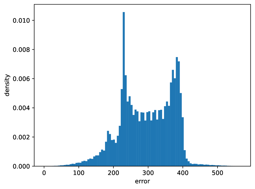
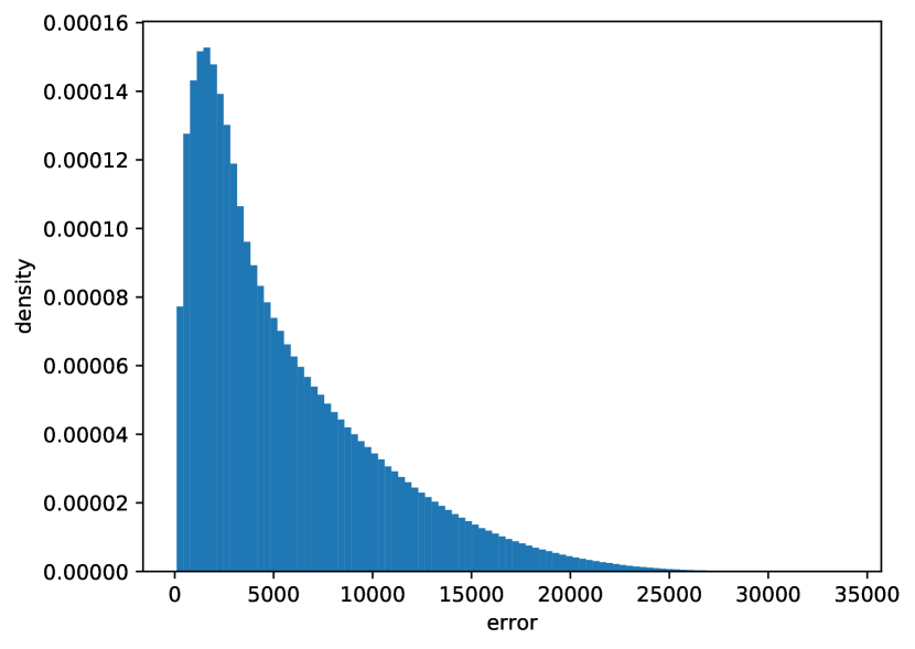
Figure 1: Distribution of $\epsilon$ for the circle (left) and the linear (right) benchmark problems

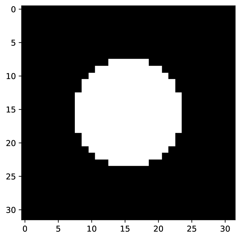
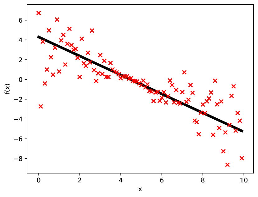
Figure 2: Example $\operatorname*{{\mathbf{x}}}_{o}$ for the circle (left) and the linear (right) benchmark problems

4.0.1 Circle image simulator

The first benchmark problem is based on a deterministic simulator of 2-dimensional circle images, while both $x$ and $y$ coordinates are constrained by the interval [-1, 1] [11]. The images are black and white, having a size of 32x32 pixels. The simulator is configured by 3 parameters $\operatorname*{{\bm{\theta}}}=(x,y,r)$, where $x$ and $y$ are the coordinates of the circle’s center, and $r$ is its radius. The true observation $\operatorname*{{\mathbf{x}}}_{o}$ is generated from $\operatorname*{{\bm{\theta}}}^{*}=(x=0,y=0,r=0.5)$ and is depicted on the left side of the Fig. 2. We assume a uniform prior with the range of [-1, 1] for $x$ and $y$ and the range of [0, 1] for $r$. Certain simulated observations from the training set of EG-LF-MCMC are able to achieve $\epsilon=0$ and exactly reproduce ${\operatorname*{{\mathbf{x}}}}_{o}$. The obtained posteriors are presented in the Fig. 3.

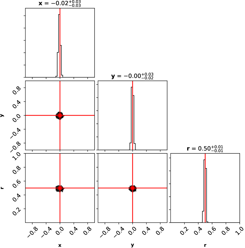
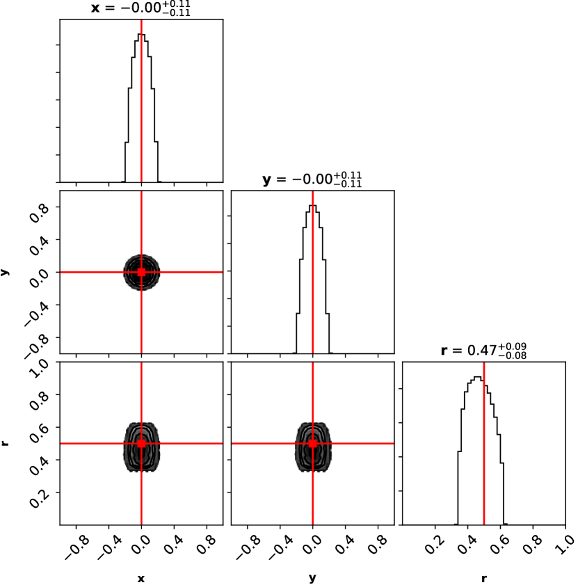
Figure 3: Posteriors for the circle problem. The true generating parameter $\operatorname*{{\bm{\theta}}}^{*}$ is depicted in red. Left: $p(\operatorname*{{\bm{\theta}}}|\epsilon)$ from EG-LF-MCMC. Right: $p(\operatorname*{{\bm{\theta}}}|\operatorname*{{\mathbf{x}}})$ from ABC

4.0.2 Stochastic linear model

Secondly, we compare the two approaches on the benchmark problem of a stochastic linear model, adapted from [8, 12]. The model is specified as:

$$y=mx+b+{\epsilon}_{1}\lvert f(mx+b)\rvert+0.05{\epsilon}_{2}$$ (5)

where ${\epsilon}_{1}$ and ${\epsilon}_{2}$ are drawn from the standard normal $\mathcal{N}(0,\,1)$. In this model $mx+b$ calculates a deterministic value for $y$ based on a standard linear function. The expression ${\epsilon}_{1}\lvert f(mx+b)\rvert$ adds a stochastic error to it based on the magnitude of $mx+b$. The term $0.05{\epsilon}_{2}$ adds a further error. We generate a 100-dimensional observation $\operatorname*{{\mathbf{x}}}_{o}$ by applying $\operatorname*{{\bm{\theta}}}^{*}=(m=-0.9594,b=4.294,f=0.534)$ and measuring the values $({y}_{1},{y}_{2},...,{y}_{100})$ at 100 equidistant $x$ points. An example $\operatorname*{{\mathbf{x}}}_{o}$ for this model is depicted on the right side of the Fig. 2. We assume a uniform prior with the range of [-5, 5] for $m$ and the range of [0, 10] for $b$ and $f$. The smallest $\epsilon$ recorded by the training set of EG-LF-MCMC is 94.7. The obtained posteriors are presented in the Fig. 4.

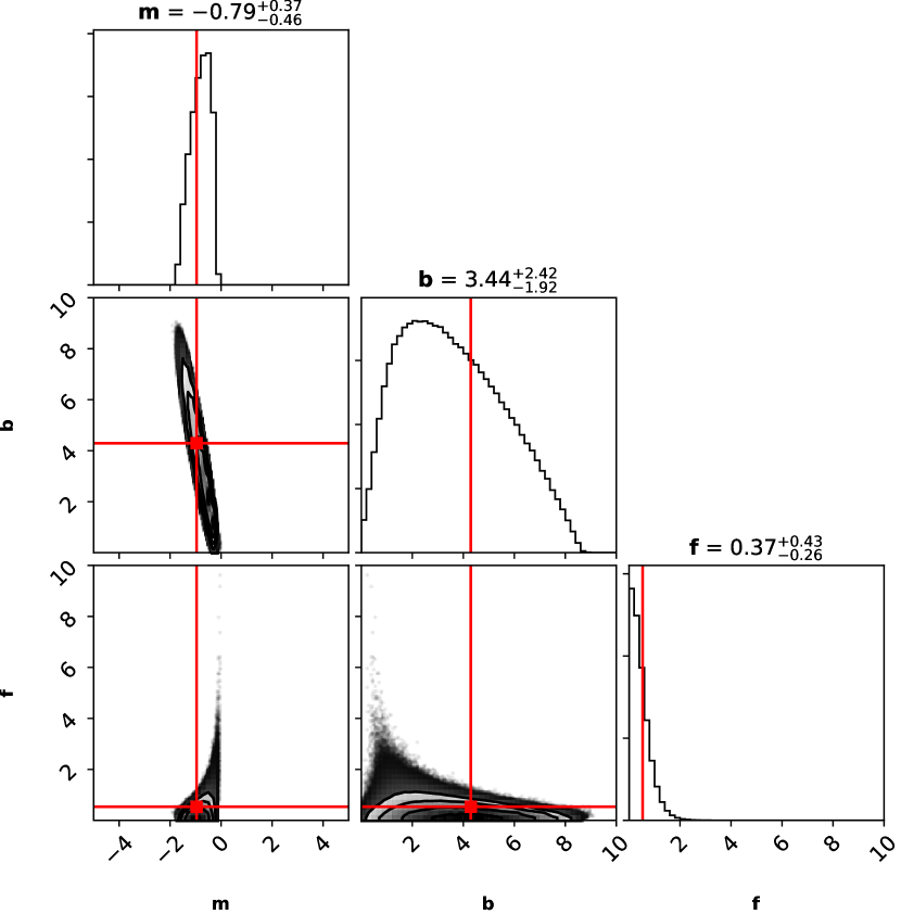
Figure 4: Posteriors for the linear problem. The true generating parameter $\operatorname*{{\bm{\theta}}}^{*}$ is depicted in red. Left: $p(\operatorname*{{\bm{\theta}}}|\epsilon)$ from EG-LF-MCMC. Right: $p(\operatorname*{{\bm{\theta}}}|\operatorname*{{\mathbf{x}}})$ from ABC

4.0.3 Discussion

Despite requiring drastically less calls to the implicit generative model, as can be seen from Table 1, the posteriors obtained by EG-LF-MCMC are significantly more certain about the true generating parameter $\operatorname*{{\bm{\theta}}}^{*}$ on both benchmark problems. Concerning the linear problem, both approaches recover $f^{*}$, but tend to underestimate it. We explain this behavior as follows. The term $f$ controls the magnitude of the stochastic error in the observations. Since ${\epsilon}_{1}$ is drawn from a standard normal, the error ${\epsilon}_{1}\lvert f(mx+b)\rvert$ can shift an observation’s value ${y}_{x}$, where $1\leq x\leq 100$, in both positive and negative directions. Thus, even if the true value $f^{*}$ is inferred, across the true observation ${\operatorname*{{\mathbf{x}}}}_{o}$ and a candidate observation $\operatorname*{{\mathbf{x}}}$ the values ${y}_{x}$ may be stochastically shifted in opposite directions, leading to a greater error. Since both EG-LF-MCMC and ABC try to infer the posteriors by minimizing the error, it is safer to assume a smaller value for $f$. This way $\operatorname*{{\mathbf{x}}}$ will stay closer to ${\operatorname*{{\mathbf{x}}}}_{o}$ on average, across different simulation runs.

4.1 Amortization over $\epsilon$

We demonstrate the ability of EG-LF-MCMC to amortize the inference over $\epsilon$, which is a completely new feature compared to AALR-MCMC. For this purpose, we turn again to the circle problem. We use the same trained classifier (amortization) as in the previously presented inference for $\operatorname*{{\bm{\theta}}}^{*}$ in order to infer approximate posterior densities for observations, which are a given distance $\epsilon$ away from $\operatorname*{{\mathbf{x}}}_{o}$. We denote such observations by $\operatorname*{{\mathbf{x}}}_{\epsilon}$. Concretely, we would like $\operatorname*{{\mathbf{x}}}_{\epsilon}$ to differ from $\operatorname*{{\mathbf{x}}}_{o}$ by 100 pixels. For this purpose, we condition the MCMC on $\epsilon=100$. The sampled multivariate chain is depicted in Fig. 5.

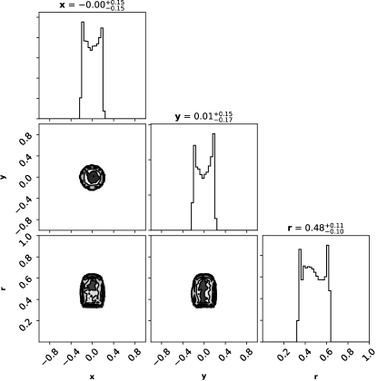
Figure 5: Circle problem: approximate posterior density $p(\operatorname*{{\bm{\theta}}}|\epsilon=100)$

The approximated posterior densities make sense semantically: in order for the images to differ by 100 pixels, $\operatorname*{{\mathbf{x}}}_{\epsilon}$ needs to be generated with the coordinates and the radius, which revolve around, but tend to diverge from $\operatorname*{{\bm{\theta}}}^{*}$. To further verify the accuracy of our approach, we draw 10,000 $\operatorname*{{\bm{\theta}}}$ samples from the resulting Markov chain, simulate respective observations $\operatorname*{{\mathbf{x}}}_{\epsilon}\sim\ p(\operatorname*{{\mathbf{x}}}|\operatorname*{{\bm{\theta}}})$ and each time record the error $\epsilon$ in relation to the true observation $\operatorname*{{\mathbf{x}}}_{o}$. Finally, we calculate the average and the standard deviation from the sample of recorded $\epsilon$ values, which turn out to be 101.46 and 3.52 respectively, confirming the accuracy of EG-LF-MCMC.

5 Conclusions and Future Work

We have presented a novel method for likelihood-free inference, named error-guided likelihood-free MCMC. It is demonstrated that EG-LF-MCMC outperforms ABC in the ability to infer the true generating model parameter $\operatorname*{{\bm{\theta}}}^{*}$ on problems with semantically and structurally different high-dimensional observational data. The circle simulator generates deterministic images, while the linear model produces stochastic numerical samples. Furthermore, we have presented the ability of EG-LF-MCMC to amortize the inference over variable $\epsilon$ values. To the best of our knowledge, this feature is novel in the likelihood-free inference literature, and it may enable novel opportunities for various scientific applications.

In the next phases of our research we plan to analytically study the connection between $p(\operatorname*{{\bm{\theta}}}|\epsilon)$ and the respective $p(\operatorname*{{\bm{\theta}}}|\operatorname*{{\mathbf{x}}})$. We hypothesize that they are equivalent when $\epsilon=0$ and in other cases $p(\operatorname*{{\bm{\theta}}}|\epsilon)$ approximates $p(\operatorname*{{\bm{\theta}}}|\operatorname*{{\mathbf{x}}})$.

References

- [1] Aeschbacher, S., Beaumont, M.A., Futschik, A.: A novel approach for choosing summary statistics in approximate bayesian computation. Genetics 192(3), 1027–1047 (2012). https://doi.org/10.1534/genetics.112.143164, https://www.genetics.org/content/192/3/1027
- [2] Beaumont, M.A., Zhang, W., Balding, D.J.: Approximate bayesian computation in population genetics. Genetics 162(4), 2025–2035 (2002), https://www.genetics.org/content/162/4/2025
- [3] Bishop, C.M.: Mixture density networks (1994), http://publications.aston.ac.uk/id/eprint/373/
- [4] Cranmer, K., Brehmer, J., Louppe, G.: The frontier of simulation-based inference. Proceedings of the National Academy of Sciences (2020). https://doi.org/10.1073/pnas.1912789117, https://www.pnas.org/content/early/2020/05/28/1912789117
- [5] Durkan, C., Murray, I., Papamakarios, G.: On contrastive learning for likelihood-free inference. International Conference on Machine Learning (2020)
- [6] Durkan, C., Papamakarios, G., Murray, I.: Sequential Neural Methods for Likelihood-free Inference. arXiv e-prints arXiv:1811.08723 (Nov 2018)
- [7] Fearnhead, P., Prangle, D.: Constructing summary statistics for approximate bayesian computation: semi-automatic approximate bayesian computation. Journal of the Royal Statistical Society: Series B (Statistical Methodology) 74(3), 419–474 (2012). https://doi.org/10.1111/j.1467-9868.2011.01010.x, https://rss.onlinelibrary.wiley.com/doi/abs/10.1111/j.1467-9868.2011.01010.x
- [8] Foreman-Mackey, D.: emcee. https://emcee.readthedocs.io/en/v2.2.1/user/line/ (2012-2013)
- [9] Greenberg, D., Nonnenmacher, M., Macke, J.: Automatic posterior transformation for likelihood-free inference. Proceedings of Machine Learning Research, vol. 97, pp. 2404–2414. PMLR, Long Beach, California, USA (09–15 Jun 2019), http://proceedings.mlr.press/v97/greenberg19a.html
- [10] Hastings, W.K.: Monte Carlo sampling methods using Markov chains and their applications. Biometrika 57(1), 97–109 (04 1970). https://doi.org/10.1093/biomet/57.1.97, https://doi.org/10.1093/biomet/57.1.97
- [11] Hermans, J., Begy, V.: Hypothesis. https://github.com/montefiore-ai/hypothesis (2019)
- [12] Hermans, J., Begy, V., Louppe, G.: Likelihood-free mcmc with amortized approximate ratio estimators. International Conference on Machine Learning (2020)
- [13] Kingma, D.P., Ba, J.: Adam: A Method for Stochastic Optimization. arXiv e-prints arXiv:1412.6980 (Dec 2014)
- [14] Klambauer, G., Unterthiner, T., Mayr, A., Hochreiter, S.: Self-normalizing neural networks. In: Guyon, I., Luxburg, U.V., Bengio, S., Wallach, H., Fergus, R., Vishwanathan, S., Garnett, R. (eds.) Advances in Neural Information Processing Systems 30, pp. 971–980. Curran Associates, Inc. (2017), http://papers.nips.cc/paper/6698-self-normalizing-neural-networks.pdf
- [15] Lueckmann, J.M., Goncalves, P.J., Bassetto, G., Öcal, K., Nonnenmacher, M., Macke, J.H.: Flexible statistical inference for mechanistic models of neural dynamics. In: Guyon, I., Luxburg, U.V., Bengio, S., Wallach, H., Fergus, R., Vishwanathan, S., Garnett, R. (eds.) Advances in Neural Information Processing Systems 30, pp. 1289–1299. Curran Associates, Inc. (2017), http://papers.nips.cc/paper/6728-flexible-statistical-inference-for-mechanistic-models-of-neural-dynamics.pdf
- [16] Marin, J.M., Pudlo, P., Robert, C.P., Ryder, R.J.: Approximate bayesian computational methods. Statistics and Computing 22(6), 1167–1180 (2012)
- [17] Metropolis, N., Rosenbluth, A.W., Rosenbluth, M.N., Teller, A.H., Teller, E.: Equation of state calculations by fast computing machines. The journal of chemical physics 21(6), 1087–1092 (1953)
- [18] Nunes, M.A., Balding, D.J.: On optimal selection of summary statistics for approximate bayesian computation. Statistical Applications in Genetics and Molecular Biology 9(1) (06 Sep 2010). https://doi.org/https://doi.org/10.2202/1544-6115.1576, https://www.degruyter.com/view/journals/sagmb/9/1/article-sagmb.2010.9.1.1576.xml.xml
- [19] Papamakarios, G., Murray, I.: Fast -free inference of simulation models with bayesian conditional density estimation. In: Advances in Neural Information Processing Systems. pp. 1028–1036 (2016)
- [20] Papamakarios, G., Sterratt, D., Murray, I.: Sequential neural likelihood: Fast likelihood-free inference with autoregressive flows. Proceedings of Machine Learning Research, vol. 89, pp. 837–848. PMLR (16–18 Apr 2019), http://proceedings.mlr.press/v89/papamakarios19a.html
- [21] Paszke, A., Gross, S., Massa, F., Lerer, A., Bradbury, J., Chanan, G., Killeen, T., Lin, Z., Gimelshein, N., Antiga, L., Desmaison, A., Kopf, A., Yang, E., DeVito, Z., Raison, M., Tejani, A., Chilamkurthy, S., Steiner, B., Fang, L., Bai, J., Chintala, S.: Pytorch: An imperative style, high-performance deep learning library. In: Wallach, H., Larochelle, H., Beygelzimer, A., d'Alché-Buc, F., Fox, E., Garnett, R. (eds.) Advances in Neural Information Processing Systems 32, pp. 8024–8035. Curran Associates, Inc. (2019), http://papers.neurips.cc/paper/9015-pytorch-an-imperative-style-high-performance-deep-learning-library.pdf