On $\beta=6$ Tracy-Widom distribution and the second Calogero-Painlevé system

A. Its

Department of Mathematical Sciences,

Indiana University – Purdue University Indianapolis

Indianapolis, IN 46202-3216, USA

St. Petersburg State University

Universitetskaya emb. 7/9

199034, St. Petersburg, Russia

A. Prokhorov

Department of Mathematics

University of Michigan

Ann Arbor, MI 48109-1043, USA

St. Petersburg State University

Universitetskaya emb. 7/9

199034, St. Petersburg, Russia

Abstract.

The Calogero-Painlevé systems were introduced in 2001 by K. Takasaki as a natural generalization of the classical Painlevé equations to the case of the several Painlevé “particles” coupled via the Calogero type interactions. In 2014, I. Rumanov discovered a remarkable fact that a particular case of the second Calogero–Painlevé II equation describes the Tracy-Widom distribution function for the general beta-ensembles with the even values of parameter beta. Most recently, in 2017 work of M. Bertola, M. Cafasso, and V. Rubtsov, it was proven that all Calogero-Painlevé systems are Lax integrable, and hence their solutions admit a Riemann-Hilbert representation. This important observation has opened the door to rigorous asymptotic analysis of the Calogero-Painlevé equations which in turn yields the possibility of rigorous evaluation of the asymptotic behavior of the Tracy-Widom distributions for the values of beta beyond the classical $\beta=1,2,4.$ In this work we shall start an asymptotic analysis of the Calogero-Painlevé system with a special focus on the Calogero-Painlevé system corresponding to $\beta=6$ Tracy-Widom distribution function.

Some technical details were omitted here and will be presented in the next version of the text.

1. Introduction and Main Result

1.1. Calogero-Painlevé system

Denote $x_{j}(t)$, $j=1,...,n$ the positions of $n$ 1D particles. The second Calogero-Painlevé model is the dynamical system given by the equations

$$x_{k}^{\prime\prime}=2x_{k}^{3}+tx_{k}+\theta+2g^{2}\sum_{j\neq k}\frac{1}{(x_{k}-x_{j})^{3}},\quad k=1,...n$$ (1.1)

These are Hamiltonian equations,

$$x^{\prime}_{k}=\frac{\partial H}{\partial y_{k}}=y_{k},\quad x^{\prime\prime}_{k}=y^{\prime}_{k}=-\frac{\partial H}{\partial x_{k}},$$

with the Hamiltonian,

$$H=\sum_{k=1}^{n}\left(\frac{y_{k}^{2}}{2}-\frac{x_{k}^{4}}{2}-\frac{x_{k}^{2}t}{2}-\theta x_{k}\right)+g^{2}\sum_{j<k}\frac{1}{(x_{k}-x_{j})^{2}}.$$ (1.2)

System (1.1) can be thought of as a collection of the n independent Painlevé II particles interacting via the classical Calogero potential. This system was introduced by K. Takasaki in 2001 [Tak], together with five other similar systems associated with each of the remaining five Painlevé equations, as non-autonomous generalization of the Inozemtsev systems [Ino]. The Calogero-Painlevé VI version of the model had also showed up in a completely different context in the work of P. Etingof, W. L. Gan, and A. Oblomkov [EGO] in connection with their study of the generalized double affine algebras of higher rank. Our principal interest in system (1.1) is its relation, discovered by I. Rumanov ( [Rum1] - [Rum3]), to the Tracy - Widom distribution function of the general beta-ensemble of random matrices.

1.2. General beta-ensemble and Calogero-Painlevé systems .

Given $\beta>0$, Dyson’s $\beta$ - ensemble is defined as a Coulomb gas of $N$ charged particles, that is as the space of $N$ one dimensional particles, $\{-\infty<\lambda_{1}<\lambda_{2}<...<\lambda_{N}<\infty\}$ with the probability density given by the equation,

$$p(\lambda_{1},\ldots,\lambda_{N})d\lambda_{1}\ldots d\lambda_{N}=\frac{1}{Z_{N}}\prod_{1\leq j,k\leq N}|\lambda_{j}-\lambda_{k}|^{\beta}{\rm e}^{-\beta\sum_{j=1}^{N}V(\lambda_{j})}d\lambda_{1}\ldots d\lambda_{N}.$$ (1.3)

$$Z_{N}=\int_{-\infty}^{\infty}...\int_{-\infty}^{\infty}\prod_{1\leq j,k\leq N}|\lambda_{j}-\lambda_{k}|^{\beta}{\rm e}^{-\beta\sum_{j=1}^{N}V(\lambda_{j})}d\lambda_{1}\ldots d\lambda_{N}$$ (1.4)

Here, $V(\lambda)$ has a meaning of external field which we will assume to be Gaussian, i.e. $V(\lambda)=\frac{\lambda^{2}}{2}$. The ensemble (1.3) has the discrete analogue (see e.g. [GH]). Correlation functions for even $\beta$ are expressed in terms of generalized special functions ( [For2], [BO]). The objects of interest are the gap probabilities in the large $N$ limit. We will be particularly concerned with the soft edge probability distribution

$$F_{\beta}(t)\equiv E_{\beta}^{\mbox{soft}}\Bigl{(}0;(t,\infty)\Bigr{)}=\lim_{N\rightarrow\infty}E_{\beta N}^{\mbox{soft}}\left(0;\Bigl{(}\sqrt{2N}+\frac{t}{\sqrt{2}N^{1/6}},\infty\Bigr{)}\right),$$ (1.5)

where

$$E_{\beta N}^{\mbox{soft}}\Bigl{(}0;(t,\infty)\Bigr{)}=\int_{-\infty}^{t}...\int_{-\infty}^{t}p(\lambda_{1},\ldots,\lambda_{N})d\lambda_{1}\ldots d\lambda_{N}.$$ (1.6)

Cases $\beta=1,2,4$ known as Gaussian orthogonal (GOE), Gaussian unitary (GUE) and Gaussian symplectic (GSE) ensembles. Indeed, in these cases, distribution (1.3) describes the statistics of the eigenvalues of orthogonal, Hermitian, and symplectic random matrices, respectively, with i.i.d. matrix entries. The corresponding limiting edge distribution functions $F_{\beta}(s)$ are then becoming the classical Tracy-Widom distributions [TW]. They admit explicit representations either as the Airy kernel Fredholm determinants or in terms of the Hastings-McLeod solution of the second Painlevé equation. These representations, in turn, allow one to evaluate the asymptotic expansions of $F_{\beta}(t)$ as $t\to\pm\infty$, i.e. the so-called tail asymptotics.

A principal issue is the asymptotic analysis of $F_{\beta}(s)$ beyond the classical values $\beta=1,2,4$. The crux of the problem is that the orthogonal polynomial approach, which is the principal technique in the random matrix case, is not available for general $\beta$. However, several highly nontrivial conjectures concerning the general $\beta$ ensembles have been suggested. An excellent presentation of the state of art in this area is given in the survey by P. Forrester [For]. The current principal heuristic result concerning the asymptotic behavior of the generalized Tracy-Widom distribution $F_{\beta}(t)$ was obtained in 2010 by G. Borot, B. Eynard, S. N. Majumdar and C. Nadal and it reads as follows.

Conjecture 1.

([BEMN])

$$F_{\beta}(t)=\exp\left(-\beta\frac{|t|^{3}}{24}+\frac{\sqrt{2}}{3}\Bigl{(}\beta/2-1\Bigr{)}|t|^{3/2}\right.$$ (1.7)

$$\left.+\frac{1}{8}\Bigl{(}\beta/2+2/\beta-3\Bigr{)}\log|t|+\chi+O\left(\frac{1}{|t|^{3/2}}\right)\right),\quad t\to-\infty,$$

The constant term $\chi$ is also explicitly predicted. Indeed, it is claimed that

$$\chi=\frac{\beta}{2}\left(\frac{1}{12}-\zeta^{\prime}(-1)\right)+\frac{\gamma}{6\beta}-\frac{\log 2\pi}{4}-\frac{\log(\beta/2)}{2}$$ (1.8)

$$+\left(\frac{17}{8}-\frac{25}{24}\Bigl{(}\beta/2+2/\beta\Bigr{)}\right)\log 2+\int_{0}^{\infty}\frac{1}{e^{\beta t/2}-1}\left(\frac{t}{e^{t}-1}-1+\frac{t}{2}-\frac{t^{2}}{12}\right)\frac{dt}{t^{2}},$$

where $\zeta(z)$ is Riemann’s zeta-function and $\gamma$ denotes Euler’s constant.

Formulae (1.7) - (1.8) have been derived in [BEMN] within the framework of the so-called loop-equation technique by performing the relevant double scaling limit directly in the formal large $N$ expansion of the multiple integral in (1.6).

Remark 1.1.

For even $\beta$ the integral above was evaluated in [BEMN]

$$\int_{0}^{\infty}\frac{1}{e^{\beta t/2}-1}\left(\frac{t}{e^{t}-1}-1+\frac{t}{2}-\frac{t^{2}}{12}\right)\frac{dt}{t^{2}}=-\sum_{m=1}^{\beta/2-1}\frac{2m}{\beta}\log\Gamma\left(\frac{2m}{\beta}\right)+\frac{2}{\beta}\zeta^{\prime}(-1)-\frac{\log(\beta/2)}{6\beta}+\frac{\beta}{8}\log(2\pi)$$

$$-\frac{\gamma}{6\beta}-\frac{\beta}{2}\left(\frac{1}{12}-\zeta^{\prime}(-1)\right).$$

Remark 1.2.

Rigorous derivation of (1.7) - (1.8) for the basic classical case $\beta=2$ is given in [DIK] and in [BBDiF]. In [BBDiF] the cases $\beta=1,4$ are also done. Both papers are using the Riemann-Hilbert method which is available to the classical cases of $\beta=1,2,4$.

Remark 1.3.

The leading asymptotic term in (1.7) for arbitrary $\beta$ has been rigorously obtained in [RRV] with the help of the analysis of the certain stochastic Schrödinger operator. We shall mention this paper again in the next paragraph.

It is remarkable, that paper [BEMN], while giving a such detailed formulae for the asymptotics of the dustribution function $F_{\beta}(t)$ does not actually produce any description of the object itself (for the finite values of $t$). The latter has been done by A. Bloemendal and B. Virag [BV]. Inspired by the pioneering work of E. Dumitriu and A. Edelman [DE] and by the subsequent works [VV] and [RRV], Bloemendal and Virag [BV] have connected the analysis of the generalized Tracy-Widom distribution $F_{\beta}(t)$ to the study of stochastic Schrödinger operators. In particular, it has been proven in [BV] that the Tracy-Widom distribution function $F_{\beta}(t)$, for any $\beta$, can be expressed in terms of the solution of a certain linear PDE. In more details, the result of [BV] can be formulated as follows.

Consider the partial differential equation,

$$\frac{\partial F}{\partial t}+\frac{2}{\beta}\frac{\partial^{2}F}{\partial x^{2}}+(t-x^{2})\frac{\partial F}{\partial x}=0,\quad(x,t)\in{\mathbb{R}}^{2}$$ (1.9)

supplemented by the boundary conditions,

$$F(x,t)\to 1,\quad\mbox{as}\quad x,t\to\infty,\quad\mbox{together}$$ (1.10)

and

$$F(x,t)\to 0,\quad\mbox{as}\quad x\to-\infty,\quad\mbox{for fixed $t$}$$ (1.11)

Theorem 1.4.

([BV]) The boundary value problem (1.9) - (1.11) has a unique bounded smooth solution. Moreover, equation,

$$F_{\beta}(t)=\lim_{x\to\infty}F(x,t),$$ (1.12)

determines the Tracy-Widom distribution function for the general value of the parameter $\beta>0$.

The next step in the studying of $F_{\beta}(t)$ has been done in the works of I. Rumanov, [Rum1] - [Rum3], who, in the case of even values of the parameter $\beta$, has reduced the analysis of the Bloemendal-Virag equation to the analysis of an auxiliary system of nonlinear ODEs. For the first nontrivial case, $\beta=6$, Rumanov has obtained the following representation for $F_{6}(t)$,

$$\log F_{6}(3^{-2/3}t)=\frac{1}{3}\int_{t}^{\infty}\Bigl{(}u^{4}(s)+su^{2}(s)-(u^{\prime}(s))^{2}\Bigr{)}ds$$

$$+\frac{2}{3}\int_{t}^{\infty}\alpha(s)ds-\frac{1}{3}\int_{t}^{\infty}\frac{u^{\prime}}{u}(s)\Bigl{(}1+\gamma(s)\Bigr{)}ds+\log\frac{1-\gamma(t)}{2}.$$ (1.13)

Here, the function $u(t)$ is the Hastings-McLeod second Painlevé transcendent, i.e. the solution of the second Painlevé equation,

$$u^{\prime\prime}=tu+2u^{3},$$ (1.14)

uniquely determined by the condition,

$$u\sim\frac{1}{2\sqrt{\pi}t^{\frac{1}{4}}}e^{-\frac{2}{3}t^{\frac{3}{2}}},\quad t\rightarrow+\infty,$$ (1.15)

while the pair of the functions $(\gamma(t),\alpha(t))$ is defined as the solution of the system of the first order ODEs,

$$\gamma^{\prime}=\frac{2}{3}\alpha\gamma+\frac{u_{t}}{u}\frac{(1+\gamma)(2-\gamma)}{3},\quad\alpha^{\prime}=\alpha\left(\frac{2}{3}\alpha+\frac{u_{t}}{u}\frac{2-\gamma}{3}\right)-\frac{t}{6}(1+\gamma)-\frac{u^{2}}{3}(3+\gamma).$$ (1.16)

with the asymptotic conditions,

$$\gamma=-1+O\left(\frac{1}{t^{\frac{3}{2}}}e^{-\frac{4}{3}t^{\frac{3}{2}}}\right),\quad\alpha=O\left(\frac{1}{t}e^{-\frac{4}{3}t^{\frac{3}{2}}}\right),\quad t\rightarrow\infty$$ (1.17)

It should be mentioned that Rumanov’s derivation of the above results based on certain heuristic assumptions which have been highlighted and some of them proven by T. Grava, A.Its, A. Kapaev, and F. Mezzadri in [GIKM]. However, the proof of a key assumption that the asymptotic conditions (1.17) determine a unique smooth solution of system (1.16), has not been yet found.

We are now going to explain the appearance in the picture of the Calogero-Painlevé system. To this end, let us pass from the triple of the functions $(u(t),\gamma(t),\alpha(t))$ to the triple $(Q_{1}(t),Q_{2}(t),Q_{3}(t))$, according to the equations,

$$e_{1}=-\frac{4\alpha\gamma}{1-\gamma^{2}}-\frac{u^{\prime}}{u}\frac{1+\gamma}{1-\gamma},\quad e_{2}=\frac{4}{1-\gamma^{2}}\left[-\alpha^{2}+u^{2}-(1+\gamma)\left(\frac{t}{2}+u^{2}+\alpha\frac{u^{\prime}}{u}\right)\right],$$

$$e_{3}=-\frac{4}{1-\gamma^{2}}\left[-2\alpha\left(\frac{t}{2}+u^{2}\right)+\alpha^{2}\frac{u^{\prime}}{u}+u^{\prime}u+\frac{1+\gamma}{2}\right],$$

where $e_{k}$ denote the first three symmetric functions of $Q_{k}$, i.e.,

$$e_{1}=Q_{1}+Q_{2}+Q_{3},\quad e_{2}=Q_{1}Q_{2}+Q_{1}Q_{3}+Q_{2}Q_{3},\quad e_{3}=Q_{1}Q_{2}Q_{3}.$$

The opposite relations are given by

$$\gamma=\mathop{\sum}_{k=1}^{3}\dfrac{-3Q_{k}^{\prime}+2\sum_{j\neq k}(Q_{k}-Q_{j})^{-1}}{\prod_{j\neq k}(Q_{k}-Q_{j})},\quad\alpha=\mathop{\sum}_{k=1}^{3}\dfrac{(-3Q_{k}^{\prime}+2\sum_{j\neq k}(Q_{k}-Q_{j})^{-1})\sum_{j\neq k}Q_{j}}{2\prod_{j\neq k}(Q_{k}-Q_{j})}-\frac{u^{\prime}}{2u}({1+\gamma}).$$

Put

$$x_{k}(t):=-6^{-1/3}Q_{k}\left(-\left(\frac{9}{2}\right)^{1/3}t\right),\quad k=1,2,3.$$

Rumanov in [Rum3] has shown that, in terms of $x_{k}(t)$, the system of the three equations (1.14), (1.16) becomes a particular case of the Calogero-Painlevé system of the three 1D interacting particles, with $\theta=-\frac{1}{6}$ and $g^{2}=-\frac{1}{9}$, i.e.,

$$x^{\prime\prime}_{k}=2x_{k}^{3}+tx_{k}-\frac{1}{6}-\frac{2}{9}\sum_{j\neq k}\frac{1}{(x_{k}-x_{j})^{3}},\quad k=1,2,3$$ (1.18)

Moreover, the asymptotic conditions (1.15), (1.17) at $t=+\infty$ are transformed into the following asymptotic condition for the functions $x_{k}(t)$ at $t=-\infty$

$$\begin{gathered}\sum_{k=1}^{3}\frac{\dfrac{\mathrm{d}x_{k}}{\mathrm{d}t}+\frac{1}{3}\sum_{j\neq k}^{3}\frac{1}{x_{k}-x_{j}}}{\prod_{j\neq k}^{3}(x_{k}-x_{j})}=1+O\left(\frac{\mathrm{e}^{-2\sqrt{2}(-t)^{\frac{3}{2}}}}{(-t)^{\frac{3}{2}}}\right),\\ \sum_{k=1}^{3}\frac{\left(\dfrac{\mathrm{d}x_{k}}{\mathrm{d}t}+\frac{1}{3}\sum_{j\neq k}^{3}\frac{1}{x_{k}-x_{j}}\right)\sum_{j\neq k}x_{j}}{\prod_{j\neq k}^{3}(x_{k}-x_{j})}=O\left(\frac{\mathrm{e}^{-2\sqrt{2}(-t)^{\frac{3}{2}}}}{t}\right).\end{gathered}$$ (1.19)

It implies that up to permutation

$$\begin{gathered}x_{1}=-\sqrt{\frac{|t|}{2}}+\frac{13}{36t}+O(|t|^{-5/2}),\quad x_{2}=\bar{x}_{3}=-\sqrt{\frac{|t|}{2}}+\frac{i}{2^{\frac{3}{4}}|t|^{\frac{1}{4}}}+\frac{4}{9t}+O(|t|^{-7/4}),\end{gathered}$$ (1.20)

The Tracy-Widom distribution $F_{6}(t)$ can be expressed directly in terms of the solution $x_{k}(t)$ of the Calogero-Painlevé system (1.18); indeed, one has that

$$\log F_{6}(-2^{-1/3}t)=\int_{-\infty}^{t}\left(H-\frac{3t^{2}}{8}+\frac{1}{2}\sum_{k=1}^{3}x_{k}\right)dt,$$ (1.21)

where,

$$H=\sum_{k=1}^{3}\left(\frac{y_{k}^{2}}{2}-\frac{x_{k}^{4}}{2}-\frac{x_{k}^{2}t}{2}+\frac{1}{6}x_{k}\right)-\frac{1}{9}\sum_{j<k}\frac{1}{(x_{k}-x_{j})^{2}},$$

is the Hamiltonian of the system (1.18) ( cf. (1.2)).

1.3. The setting of the asymptotic problem for the Calogero-Painlevé system

The Borot-Eynard-Majumdar-Nadal conjecture (1.7) in the case of $\beta=6$ reads

$$\log F_{6}(t)=-\frac{1}{4}|t|^{3}+\frac{2\sqrt{2}}{3}|t|^{\frac{3}{2}}+\frac{1}{24}\log|t|+\chi+O(t^{-3/2}),\quad t\to-\infty$$ (1.22)

The ultimate goal of our study is to prove this formula using the representation (1.13) for the function $F_{6}(t)$. To this end, one needs to find the asymptotics at $t=-\infty$ of the solution $(\gamma(t),\alpha(t))$) of the system (1.16) which behaves at $t=+\infty$ as it is indicated in (1.17). Taking into account the known behavior of the Hastngs-Mcleod Painlevé function $u(t)$ as $t\to-\infty$, i.e.,

$$u(t)=\sqrt{\frac{|t|}{2}}\left(1+\frac{1}{8}t^{-3}+O(t^{-6})\right),\quad t\to-\infty,$$ (1.23)

one can check that the system (1.16) admits the formal solution with the asymptotics,

$$\gamma=\frac{1}{\sqrt{2}}|t|^{-\frac{3}{2}}-\frac{21}{8}t^{-3}+\frac{1707}{64\sqrt{2}}|t|^{-\frac{9}{2}}+O(t^{-6}),\quad\alpha=\frac{1}{\sqrt{2}}|t|^{\frac{1}{2}}+\frac{1}{8}t^{-1}-\frac{37}{64\sqrt{2}}|t|^{-\frac{5}{2}}+O(t^{-4}),$$ (1.24)

as $t\to-\infty$. It is significant, that the asymptotics (1.23), (1.24) generate via (1.13) the asymptotic formula (1.22) (without though the constant term $\chi$). Hence, a key question to address is to show that the solution $(\gamma(t),\alpha(t))$) of the system (1.16) fixed by the behavior (1.17) at $t=+\infty$ has indeed the asymptotics (1.24), at $t=-\infty$. Another words, one needs to find a connection formulae for the solution $(\gamma(t),\alpha(t))$ of system (1.16).

Notice, that the $t=-\infty$ asymptotic formulae (1.23) - (1.24), in terms of the Calogero-Painlevé coordinates $x_{j}$, become the following asymptotic relations at $t=+\infty$ up to permutation,

$$x_{1}=\frac{1}{6t}+\frac{8}{27t^{\frac{5}{2}}}+O(t^{-4}),\quad x_{2}=\bar{x}_{3}=\frac{i\sqrt{2}}{2t^{\frac{1}{4}}}+\frac{1}{6t}+O(t^{-\frac{5}{2}}),\quad t\to+\infty.$$ (1.25)

Therefore, we arrive at the following connection problem for the Calogero-Painlevé system (1.18):

Show that there is a unique solution, $(x_{1}(t),x_{2}(t),x_{3}(t))$, of (1.18) which is smooth for all real $t$ and which behaves at $t=-\infty$ and $t=+\infty$ as it is indicated in equations (1.20) and (1.25), respectively, up to permutation.

We are going to address this problem using the Riemann-Hilbert representation of the solutions of the Calogero-Painlevé system which was found in the recent work [BCR] and which we will now describe in some details.

1.4. The Riemann-Hilbert representation of the Calogero-Painlevé particles.

In [BCR], it is shown (in fact, for the general case of $n$ particles) that the system (1.18) is Lax-pair integrable, and the following Riemann-Hilbert representation of its general solution takes place.

Riemann-Hilbert problem 1.5.

Denote $\Gamma_{j}$ , $j=1,2,3,4,5,6$ the rays $\arg z=\frac{\pi}{6}(2j-1)$, $j=1,2,3$ and $\arg z=-2\pi+\frac{\pi}{6}(2j-1)$, $j=4,5,6$ oriented toward infinity, and also denote ${\mathbb{R}}_{-}$ the half real line, $z<0$ oriented to the left (see Figure 1). Let now set the Riemann-Hilbert problem consisting in finding the $6\times 6$ matrix valued function $\Psi(z;t)$ such that

• $\Psi(z)$ is holomorphic on ${\mathbb{C}}\setminus\{{\mathbb{R}}_{-}\cup\Bigl{(}\cup_{j=1}^{6}\Gamma_{j}\Bigr{)}\}$, and the boundary values, $\Psi_{\pm}(z)$, are finite and satisfy the following jump conditions,

  $$\Psi_{+}(z)=\Psi_{-}(z)S_{j},\quad z\in\Gamma_{j},\quad j=1,...,6,\quad\Psi_{+}(z)=\Psi_{-}(z)e^{-\frac{2\pi i}{3}}I_{6}\quad z\in{\mathbb{R}}_{-}$$ (1.26)

• The behavior of  $\Psi(z)$ as $z\to\infty,0$ is described by the equations,

  $$\Psi(z)=\left(I_{6}+\frac{m_{1}}{z}+O\left(\frac{1}{z^{2}}\right)\right)z^{I_{2}\otimes\Lambda_{1}}e^{\frac{i}{2}\left(\frac{z^{3}}{3}+tz\right)\sigma_{3}\otimes I_{3}},\quad z\to\infty,$$ (1.27)

  and

  $$\Psi(z)=G_{0}\Bigl{(}I_{6}+O(z)\Bigr{)}z^{\frac{1}{6}\sigma_{3}\otimes I_{3}}E,\quad z\to 0,\quad|\arg z|<\frac{\pi}{6}.$$ (1.28)

Here,

$$\sigma_{3}=\begin{pmatrix}1&0\cr 0&-1\end{pmatrix},\quad\Lambda_{1}=\begin{pmatrix}-\frac{2}{3}&0&0\cr 0&\frac{1}{3}&0\cr 0&0&\frac{1}{3}\end{pmatrix}.$$

and $S_{j}$ are the block-triangular matrices,

$$S_{1}=\left(\begin{array}[]{cc}I_{3}&A\\ 0&I_{3}\end{array}\right),\quad S_{2}=\left(\begin{array}[]{cc}I_{3}&0\\ B&I_{3}\end{array}\right),\quad S_{3}=\left(\begin{array}[]{cc}I_{3}&C\\ 0&I_{3}\end{array}\right),$$

$$S_{4}=\left(\begin{array}[]{cc}I_{3}&0\\ e^{i\pi\Lambda_{1}}Ae^{-i\pi\Lambda_{1}}&I_{3}\end{array}\right),\quad S_{5}=\left(\begin{array}[]{cc}I_{3}&e^{i\pi\Lambda_{1}}Be^{-i\pi\Lambda_{1}}\\ 0&I_{3}\end{array}\right),\quad S_{6}=\left(\begin{array}[]{cc}I_{3}&0\\ e^{i\pi\Lambda_{1}}Ce^{-i\pi\Lambda_{1}}&I_{3}\end{array}\right).$$

We denote by $I_{n}$ the identity matrix in $\mathbb{R}^{n}$.

Figure 1. Contour for the Riemann-Hilbert problem 1.5

The $3\times 3$ matrices $A$, $B$, and $C$ are satisfying certain algebraic relations (see equations (3.1) in Section 3.2) which are the consequence of the cyclic equation,

$$E^{-1}e^{-\frac{\pi i}{3}\sigma_{3}\otimes I_{3}}E=e^{-\frac{2\pi i}{3}}S_{1}S_{2}S_{3}S_{4}S_{5}S_{6}.$$ (1.29)

which also determines the matrix factor $E$ in (1.28). Having solution $\Psi(z)$, the solutions $x_{k}(t)$ of the Calogero - Painlevé system are determined as the eigenvalues of the $3\times 3$ matrix

$$iq_{0}(t)=\hat{m}_{1,12},$$ (1.30)

where $\hat{m}_{1,12}$ denote the $3\times 3$ up-right block of the coefficient $6\times 6$ matrix $m_{1}$ from the expansion (1.27).

The first principal question now is which Riemann-HIlbert data, i.e. the matrices $A$, $B$ and $C$, yield the solution of the Calogero - Painlevé system (1.18) that corresponds to the Tracy-Widom function $F_{6}(t)$. The main result of this paper is the following partial answer to this question.

Theorem 1.6.

Let the Riemann-Hilbert data are chosen according to the equations,

$$A=\left(\begin{array}[]{ccc}a&\sqrt{3}ab_{1}e^{-\frac{5\pi i}{6}}&{\sqrt{3}e^{\frac{5\pi i}{6}}{}}\\ 0&e^{-\frac{5\pi i}{6}}-a^{-1}&0\\ 0&{\sqrt{3}e^{-\frac{5\pi i}{6}}{}}&e^{-\frac{\pi i}{3}}a\end{array}\right),\quad B=\left(\begin{array}[]{ccc}0&b_{2}&b_{1}\\ 0&0&1\\ 1&{b_{1}{}}&0\end{array}\right),\quad C=\left(\begin{array}[]{ccc}e^{\frac{\pi i}{3}}a+e^{\frac{\pi i}{6}}&\frac{1}{a}\sqrt{3}b_{1}e^{-\frac{\pi i}{6}}&{\sqrt{3}e^{-\frac{5\pi i}{6}}{}}\\ 0&{e^{\frac{2\pi i}{3}}}{a^{-1}}&0\\ 0&{\sqrt{3}e^{\frac{5\pi i}{6}}{}}&{e^{-\frac{2\pi i}{3}}}{a^{-1}}\end{array}\right),$$ (1.31)

where $a,b_{1},b_{2}$ are complex parameters. They are determined up to conjugation by the same constant matrix. Then the following statements are true.

1. The solution $\Psi(z)\equiv\Psi(z,t)$ and the corresponding $3\times 3$ matrix $q_{0}(t)$ from (1.30) exist as meromorphic functions of $t$.

2. Take $a=i$. Then the eigenvalues

   $$\Bigl{(}x_{1}(t),x_{2}(t),x_{3}(t)\Bigr{)}\equiv\Bigl{(}x_{1}(t;b_{1},b_{2}),x_{2}(t;b_{1},b_{2}),x_{3}(t;b_{1},b_{2})\Bigr{)}$$

   of the matrix $q_{0}(t)$ determine a family of solutions of the Calogero-Painlevé system (1.18) whose behavior as $t\to-\infty$ is given by the asymptotic formulae (1.20) up to permutation.

3. Take $b_{1}=b_{2}=0$, $a\in\{i,e^{-\frac{5\pi i}{6}}\}$. Then the eigenvalues $\Bigl{(}x_{1}(t),x_{2}(t),x_{3}(t)\Bigr{)}$ of the matrix $q_{0}(t)$ determine solutions of the Calogero-Painlevé system (1.18) whose behavior as $t\to+\infty$ is given by the asymptotic formulae (1.25) up to permutation.

The still open questions are:

• To show that the choice (1.31) guarantees that the Riemann-Hilbert problem is solvable for all real $t$ and the corresponding solution $(x_{1}(t),x_{2}(t),x_{3}(t))$ of the Calogero-Painlevé system is also exists and is smooth for all real $t$.

• To show that the choice $a=i,\,b_{1}=0,\,b_{2}=0$ indeed yields the solution $(x_{1}(t),x_{2}(t),x_{3}(t))$ which generates the Tracy- Widom distribution $F_{6}(t)$ and hence to prove the BEMN conjecture (1) for $\beta=6$ (without the constant term $\chi$.) The issue here is that asymptotics (1.20) by itself do not define the solution $(x_{1}(t),x_{2}(t),x_{3}(t))$ uniquely - there is an “unseen” exponentially small term in it, and hence it can not be easily transformed back to the asymptotics (1.19). The best we can get is the power decay instead of the exponential decay. Presumably, the second asymptotics, i.e. formula (1.25), fixes the solution uniquely.

• To evaluate rigorously $\chi$.

• To extend the result to arbitrary even $\beta$.

We intend to address all these questions in the forthcoming publication.

1.5. Plan of the paper

In the next section - Section 2, we shall present, following [BCR], the isomonodromy Lax pair for the Calogero-Painlevé system (1.18). Then, in the beginning of Section 3, following again [BCR], we will transform the Lax formalism for the Calogero-Painlevé system to its Riemann-Hilbert formalism. The main body of the paper consists of Subsections 3.1 and 3.2 where we perform the asymptotic analysis of the Bertola-Cafasso-Rubtsov Riemann-Hilbert problem as $t\to+\infty$ and $t\to-\infty$, respectively. The specific structure of the jump matrices announced in Theorem 1.6 will be fixed in a process of application of the Deift - Zhou nonlinear steepest descent method which will eventually lead us to the proof of the Theorem. It should be noticed that the nonlinear steepest descent analysis in the case under consideration is rather tricky because of the high matrix size of the Riemann-Hilbert problem. In fact, and we will say more about that later on, the Riemann-Hilbert we are dealing with is a non-abelian version of the Flaschka-Newell Lax pair for the second Painlevé equation.

2. Lax pair of the Calogero-Painlevé System

2.1. Matrix Painlevé equation

The following Lax pair considered in [BCR] is the quantization of Flaschka-Newell pair for the second Painlevé equation

$$\dfrac{dW}{dz}=U(z)W(z),\quad\dfrac{dW}{dt}=V(z)W(z),$$ (2.1)

$$U(z)=U_{2}z^{2}+U_{1}z+U_{0}+\dfrac{U_{-1}}{z},\quad V(z)=V_{1}z+V_{0},$$

$$U_{2}=\left(\begin{array}[]{cc}\dfrac{iI_{3}}{2}&0\\ 0&-\dfrac{iI_{3}}{2}\end{array}\right),\quad U_{1}=\left(\begin{array}[]{cc}0&q\\ q&0\end{array}\right),\quad U_{0}=\left(\begin{array}[]{cc}iq^{2}+\dfrac{itI_{3}}{2}&-ip\\ ip&-iq^{2}-\dfrac{itI_{3}}{2}\end{array}\right),\quad U_{-1}=\left(\begin{array}[]{cc}0&-\theta I_{3}\\ -\theta I_{3}&0\end{array}\right)$$

$$V_{1}=U_{2},\quad V_{0}=U_{1}.$$

Here $q$ and $p$ are $3\times 3$ matrices, compared to standard Flaschka-Newell Lax pair. The compatibility condition takes form of matrix Painlevé II equation

$$\dfrac{dq}{dt}=p,\quad\dfrac{dp}{dt}=2q^{3}+tq+\theta I_{3}.$$ (2.2)

The symmetry of the coefficient matrix

$$-U(-z)=({\sigma}_{1}\otimes I_{3})U(z)({\sigma}_{1}\otimes I_{3}).$$

implies the symmetry of solution

$$W(-z)=(\sigma_{1}\otimes I_{3})W(z)(\sigma_{1}\otimes I_{3}).$$ (2.3)

We have the following asymptotic at infinity

$$W(z)=\left(I_{6}+\dfrac{n_{1}}{z}+O\left(\dfrac{1}{z^{2}}\right)\right)e^{(\ln z+i\pi\varepsilon)(I_{2}\otimes[q,p])}e^{\frac{i}{2}\left(\frac{z^{3}}{3}+tz\right)(\sigma_{3}\otimes I_{3})},$$ (2.4)

where

$$\varepsilon=\begin{cases}0&\mathrm{Im}(z)\geq 0\\ 1&\mathrm{Im}(z)<0\\ \end{cases},\quad\hat{n}_{1,12}=iq.$$

The asymptotic at the origin has form

$$W(z)=G_{0}\left(I_{6}+O\left(z\right)\right)e^{(\ln z+i\pi\varepsilon){(-\theta\sigma_{3}\otimes I_{3})}}(K\otimes I_{3})^{-1},\quad z\to 0,$$ (2.5)

with

$$G_{0}=(K\otimes I_{3})\begin{pmatrix}r_{1}&0\\ 0&r_{2}\\ \end{pmatrix},\quad K=\dfrac{1}{\sqrt{2}}\left(\begin{array}[]{cc}1&-1\\ 1&1\end{array}\right),\quad K\sigma_{3}=\sigma_{1}K,\quad\sigma_{3}K=-K\sigma_{1}.$$

We can see that the symmetry (2.3) is preserved in equations (2.5), (2.4). We would like to notice that the choice of $g=\pm\frac{i}{3}$ makes the operator $\mathrm{Id}+\mathrm{ad}_{[q,p]}$ not invertible and to find $m_{1}$ we would need to use standard procedure presented in [FIKN] and not in [BCR].

The $3\times 3$ matrices $r_{1}$ and $r_{2}$ satisfy the equations

$$\dfrac{dr_{1}}{dt}=qr_{1},\quad\dfrac{dr_{2}}{dt}=-qr_{2}.$$

2.2. Calogero-Painlevé system of equations

The commutator $[p,q]$ is preserved by dynamics (2.2), so it is part of monodromy data. We will need to choose it from Calogero-Moser space

$$[p,q]=ig(I_{3}-v^{T}v)=-ig\left(\begin{array}[]{ccc}0&1&1\\ 1&0&1\\ 1&1&0\end{array}\right),\quad v=(1,1,\ldots,1).$$

Below we list the results from [BCR]. It is possible to conjugate matrices $q$ and $p$ in such a way that

$$q=\mathcal{O}X\mathcal{O}^{-1},\quad X=\left(\begin{array}[]{ccc}x_{1}&0&0\\ 0&x_{2}&0\\ 0&0&x_{3}\end{array}\right),$$

$$p=\mathcal{O}Y\mathcal{O}^{-1},\quad Y=\left(\begin{array}[]{ccc}y_{1}&\dfrac{ig}{(x_{1}-x_{2})}&\dfrac{ig}{(x_{1}-x_{3})}\\ \dfrac{ig}{(x_{2}-x_{1})}&y_{2}&\dfrac{ig}{(x_{2}-x_{3})}\\ \dfrac{ig}{(x_{3}-x_{1})}&\dfrac{ig}{(x_{3}-x_{2})}&y_{3}\end{array}\right).$$

The eigenvectors of $q$ forming matrix $\mathcal{O}$ satisfy the equation $\dfrac{d\mathcal{O}}{dt}=\mathcal{O}F$ with

$$F=\left(\begin{array}[]{ccc}f_{1}&-\dfrac{ig}{(x_{1}-x_{2})^{2}}&-\dfrac{ig}{(x_{1}-x_{3})^{2}}\\ -\dfrac{ig}{(x_{2}-x_{1})^{2}}&f_{2}&-\dfrac{ig}{(x_{2}-x_{3})^{2}}\\ -\dfrac{ig}{(x_{3}-x_{1})^{2}}&-\dfrac{ig}{(x_{3}-x_{2})^{2}}&f_{3}\end{array}\right),$$

$$f_{1}=-\dfrac{2ig}{3}\dfrac{1}{(x_{2}-x_{3})^{2}}+\dfrac{ig}{3}\dfrac{1}{(x_{1}-x_{3})^{2}}+\dfrac{ig}{3}\dfrac{1}{(x_{2}-x_{1})^{2}},$$

$$f_{2}=-\dfrac{2ig}{3}\dfrac{1}{(x_{1}-x_{3})^{2}}+\dfrac{ig}{3}\dfrac{1}{(x_{2}-x_{3})^{2}}+\dfrac{ig}{3}\dfrac{1}{(x_{2}-x_{1})^{2}},$$

$$f_{3}=-\dfrac{2ig}{3}\dfrac{1}{(x_{2}-x_{1})^{2}}+\dfrac{ig}{3}\dfrac{1}{(x_{1}-x_{3})^{2}}+\dfrac{ig}{3}\dfrac{1}{(x_{2}-x_{3})^{2}}.$$

Taking it into account, one can rewrite the compatibility conditions (2.2) as

$$\dfrac{dX}{dt}=Y+[X,F],\quad\dfrac{dY}{dt}=2X^{3}+tX+\theta I_{3}+[Y,F].$$

It implies that eigenvalues of matrix $q$ satisfy Calogero Painlevé system of equations (1.1).

3. Riemann-Hilbert problem

The case of $\beta=6$ Tracy-Widom law corresponds to $g^{2}=-\frac{1}{9},\,\theta=-\frac{1}{6}$. We choose $g=\frac{i}{3},\,\theta=-\frac{1}{6}$ from now on.

Consider the following Riemann-Hilbert problem.

Riemann-Hilbert problem 3.1.

Consider the contour $\Gamma$ shown on Figure 2. The $6\times 6$ matrix valued function $W(z)$ satisfies the following conditions

• $W(z)$ is holomorphic on $\mathbb{C}\setminus\Gamma$.

• $W(z)$ has finite boundary values on the contour $\Gamma$ and satisfies the jump condition indicated on Figure 2 with

  $$L=(K\otimes I_{3})e^{-\frac{\pi i(\sigma_{3}\otimes I_{3})}{6}}(K\otimes I_{3})^{-1},$$

  $$S_{1}=\left(\begin{array}[]{cc}I_{3}&A\\ 0&I_{3}\end{array}\right),\quad S_{2}=\left(\begin{array}[]{cc}I_{3}&0\\ B&I_{3}\end{array}\right),\quad S_{3}=\left(\begin{array}[]{cc}I_{3}&C\\ 0&I_{3}\end{array}\right),$$

  $$\widetilde{S}_{4}=\left(\begin{array}[]{cc}I_{3}&0\\ A&I_{3}\end{array}\right),\quad\widetilde{S}_{5}=\left(\begin{array}[]{cc}I_{3}&B\\ 0&I_{3}\end{array}\right),\quad\widetilde{S}_{6}=\left(\begin{array}[]{cc}I_{3}&0\\ C&I_{3}\end{array}\right),$$

  Matrix $E_{0}$ is chosen based on cyclic condition

  $${S}_{1}{S}_{2}{S}_{3}e^{-i\pi(I_{2}\otimes[q,p])}\widetilde{S}_{4}\widetilde{S}_{5}\widetilde{S}_{6}e^{-i\pi(I_{2}\otimes[q,p])}=E_{0}(K\otimes I_{3})e^{-\frac{\pi i(\sigma_{3}\otimes I_{3})}{3}}(K\otimes I_{3})^{-1}E_{0}^{-1}$$

  It can be selected up to right multiplication by block diagonal matrix, which corresponds to the fixing of extra functions $r_{1}$ and $r_{2}$. We are not concerned about them, so we do not specify this choice.

  The jumps on other arcs of the circle can be derived from $E_{0}$ using cyclic relations around the points of intersection on the circle.

• function $W(z)$ have the asymptotics (2.4), (2.5) at infinity and at zero respectively.

Solution $W(z)$ of the Riemann-Hilbert problem 3.1 satisfies Lax pair equations (2.1) and symmetry condition (2.3).

Figure 2. Contour for the Riemann-Hilbert problem 3.1

The commutator $[q,p]$ can be diagonalized. We have

$$P_{1}^{-1}[q,p]P_{1}=\Lambda_{1},\quad\Lambda_{1}=\left(\begin{array}[]{ccc}-\frac{2}{3}&0&0\\ 0&\frac{1}{3}&0\\ 0&0&\frac{1}{3}\end{array}\right),\quad P_{1}=\left(\begin{array}[]{ccc}\frac{1}{\sqrt{3}}&\frac{2}{\sqrt{6}}&0\\ \frac{1}{\sqrt{3}}&-\frac{1}{\sqrt{6}}&-\frac{1}{\sqrt{2}}\\ \frac{1}{\sqrt{3}}&-\frac{1}{\sqrt{6}}&\frac{1}{\sqrt{2}}\\ \end{array}\right).$$

Conjugating $W(z)$ by $I_{2}\otimes P_{1}$ we can diagonalize the commutator in the Riemann-Hilbert problem. We also rearrange the jump near zero and infinity using matrix $M_{1}$

$$H(z)=(I_{2}\otimes P_{1})^{-1}W(z)(I_{2}\otimes P_{1})M_{1}$$

Figure 3. Matrix $M_{1}$

That lead us to the new Riemann-Hilbert problem for $H(z)$.

Riemann-Hilbert problem 3.2.

Consider the contour $\Gamma$ shown on Figure 4. The $6\times 6$ matrix valued function $H(z)$ satisfies the following conditions

• $H(z)$ is holomorphic on $\mathbb{C}\setminus\Gamma$.

• $H(z)$ has finite boundary values on the contour $\Gamma$ and satisfies the jump condition indicated on Figure 4 with

  $$E=(E_{0}(K\otimes I_{3}))^{-1},\quad S_{4}=\left(\begin{array}[]{cc}I_{3}&0\\ e^{i\pi\Lambda_{1}}Ae^{-i\pi\Lambda_{1}}&I_{3}\end{array}\right),\quad S_{5}=\left(\begin{array}[]{cc}I_{3}&e^{i\pi\Lambda_{1}}Be^{-i\pi\Lambda_{1}}\\ 0&I_{3}\end{array}\right),\quad S_{6}=\left(\begin{array}[]{cc}I_{3}&0\\ e^{i\pi\Lambda_{1}}Ce^{-i\pi\Lambda_{1}}&I_{3}\end{array}\right),$$

• $H(z)$ have the following behavior at infinity

  $$H(z)=\left(I_{6}+\dfrac{m_{1}}{z}+O\left(\dfrac{1}{z^{2}}\right)\right)z^{I_{2}\otimes\Lambda_{1}}e^{\frac{i}{2}\left(\frac{z^{3}}{3}+tz\right)(\sigma_{3}\otimes I_{3})},\quad z\to\infty,$$

  and at zero

  $$H(z)=(K\otimes I_{3})\left(\begin{array}[]{cc}P_{1}^{-1}r_{1}P_{1}&0\\ 0&P_{1}^{-1}r_{2}P_{1}\end{array}\right)\left(I_{6}+O\left(z\right)\right)z^{\frac{\sigma_{3}\otimes I_{3}}{6}},\quad z\to 0,$$

Here

$$m_{1}=(I_{2}\otimes P_{1})^{-1}n_{1}(I_{2}\otimes P_{1})$$

and we have the relation (1.30) with

$$q_{0}(t)=P_{1}^{-1}q(t)P_{1}.$$

Figure 4. Contour for the Riemann-Hilbert problem 3.2

The function $H(z)$ differs from function $\Psi(z)$ described in Riemann-Hilbert problem 1.5 only by extra multiplication by matrix $E$ near the origin.

The cyclic relation (1.29) written componentwise takes form

$$\begin{gathered}(A+C+ABC)e^{-i\pi\Lambda_{1}}+e^{i\pi\Lambda_{1}}B+iI_{3}=0,\\ (AB+I_{3})e^{-i\pi\Lambda_{1}}-e^{i\pi\Lambda_{1}}(BA+I_{3})=0,\\ Ce^{-i\pi\Lambda_{1}}A-Ae^{i\pi\Lambda_{1}}C+e^{-i\pi\Lambda_{1}}-e^{i\pi\Lambda_{1}}=0,\\ (BC+I_{3})e^{-i\pi\Lambda_{1}}-e^{i\pi\Lambda_{1}}(CB+I_{3})=0,\\ Be^{-i\pi\Lambda_{1}}+e^{i\pi\Lambda_{1}}(A+C+CBA)+iI_{3}=0.\end{gathered}$$ (3.1)

We will look for matrices $A,B,C$ in the form

$$A=\left(\begin{array}[]{ccc}a_{1}&a_{6}&a_{5}\\ 0&a_{2}&0\\ 0&a_{4}&a_{3}\end{array}\right),\quad{B}=\left(\begin{array}[]{ccc}0&b_{2}&b_{1}\\ 0&0&b_{4}\\ b_{3}&b_{5}&0\end{array}\right),\quad C=\left(\begin{array}[]{ccc}c_{1}&c_{6}&c_{5}\\ 0&c_{2}&0\\ 0&c_{4}&c_{3}\end{array}\right)$$ (3.2)

The motivation for this choice is the needs of asymptotic analysis and it is mentioned at the end of sections 3.1.1, and 3.2.1. We get the following solution:

$$A=\left(\begin{array}[]{ccc}a&\frac{1}{b_{3}b_{4}}\sqrt{3}ab_{1}e^{-\frac{5\pi i}{6}}&\frac{\sqrt{3}e^{\frac{5\pi i}{6}}}{b_{3}}\\ 0&e^{-\frac{5\pi i}{6}}-a^{-1}&0\\ 0&\frac{\sqrt{3}e^{-\frac{5\pi i}{6}}}{b_{4}}&e^{-\frac{\pi i}{3}}a\end{array}\right),\quad B=\left(\begin{array}[]{ccc}0&\frac{b_{2}}{b_{3}b_{4}}&\frac{b_{1}}{b_{3}}\\ 0&0&b_{4}\\ b_{3}&\frac{b_{1}}{b_{4}}&0\end{array}\right),\quad C=\left(\begin{array}[]{ccc}e^{\frac{\pi i}{3}}a+e^{\frac{\pi i}{6}}&\frac{1}{ab_{3}b_{4}}\sqrt{3}b_{1}e^{\frac{-\pi i}{6}}&\frac{\sqrt{3}e^{-\frac{5\pi i}{6}}}{b_{3}}\\ 0&{e^{\frac{2\pi i}{3}}}{a^{-1}}&0\\ 0&\frac{\sqrt{3}e^{\frac{5\pi i}{6}}}{b_{4}}&{e^{-\frac{2\pi i}{3}}}{a^{-1}}\end{array}\right),$$

with $a\in\{i,e^{-\frac{5\pi i}{6}}\}$.

Performing conjugation $A,B,C\to\Lambda_{2}^{-1}A\Lambda_{2},\Lambda_{2}^{-1}B\Lambda_{2},\Lambda_{2}^{-1}C\Lambda_{2}$ with

$$\Lambda_{2}=\begin{pmatrix}b_{3}^{-\frac{2}{3}}b_{4}^{-\frac{1}{3}}&0&0\\ 0&b_{3}^{\frac{1}{3}}b_{4}^{\frac{2}{3}}&0\\ 0&0&b_{3}^{\frac{1}{3}}b_{4}^{-\frac{1}{3}}\end{pmatrix}$$

we cancel $b_{3}$ and $b_{4}$. This operation corresponds to conjugation of solution $H(z)\to(I_{2}\otimes\Lambda_{2})^{-1}H(z)(I_{2}\otimes\Lambda_{2})$. Therefore we arrived to the monodromy data (1.31).

It is worth mentioning that performing conjugation $A,B,C\to P_{4}^{-1}AP_{4},P_{4}^{-1}BP_{4},P_{4}^{-1}CP_{4}$ with

$$P_{4}=\begin{pmatrix}0&0&1\\ 1&0&0\\ 0&1&0\end{pmatrix}$$

we get matrices to be more symmetric:

$$A=\left(\begin{array}[]{ccc}e^{-\frac{5\pi i}{6}}-a^{-1}&0&0\\ {\sqrt{3}e^{-\frac{5\pi i}{6}}}&e^{-\frac{\pi i}{3}}a&0\\ \sqrt{3}ab_{1}e^{-\frac{5\pi i}{6}}&{\sqrt{3}e^{\frac{5\pi i}{6}}}&a\end{array}\right),\quad B=\left(\begin{array}[]{ccc}0&1&0\\ {b_{1}{}}&0&1\\ {b_{2}{}}&{b_{1}{}}&0\end{array}\right),\quad C=\left(\begin{array}[]{ccc}{e^{\frac{2\pi i}{3}}}{a^{-1}}&0&0\\ {\sqrt{3}e^{\frac{5\pi i}{6}}}&{e^{-\frac{2\pi i}{3}}}{a^{-1}}&0\\ \frac{1}{a}\sqrt{3}b_{1}e^{\frac{-\pi i}{6}}&{\sqrt{3}e^{-\frac{5\pi i}{6}}{}}&e^{\frac{\pi i}{3}}a+e^{\frac{\pi i}{6}}\end{array}\right).$$

3.1. Asymptotic $t\to+\infty$

For this asymptotic we put $b_{1}=b_{2}=0$.

3.1.1. Preliminary transformations

Consider scaling change of variables

$$\Phi(\lambda)=t^{-\frac{1}{2}I_{2}\otimes\Lambda_{1}}H(\lambda\sqrt{t})$$

We have the behavior at infinity and zero changed to

$$\Phi(\lambda)=\left(I+O\left(\dfrac{1}{\lambda}\right)\right)\lambda^{I_{2}\otimes\Lambda_{1}}e^{\frac{i}{2}t^{\frac{3}{2}}\left(\frac{\lambda^{3}}{3}+\lambda\right)({\sigma}_{3}\otimes I_{3})},\quad\lambda\to\infty,$$ (3.3)

$$\Phi(\lambda)=(K\otimes I_{3})\left(\begin{array}[]{cc}t^{-\frac{\Lambda_{1}}{2}}P_{1}^{-1}r_{1}P_{1}t^{\frac{\Lambda_{1}}{2}}&0\\ 0&t^{-\frac{\Lambda_{1}}{2}}P_{1}^{-1}r_{2}P_{1}t^{\frac{\Lambda_{1}}{2}}\end{array}\right)\left(I_{6}+O\left(\lambda\right)\right)\lambda^{\frac{\sigma_{3}\otimes I_{3}}{6}}t^{-\frac{1}{2}I_{2}\otimes\Lambda_{1}+\frac{1}{12}\sigma_{3}\otimes I_{3}},\quad\lambda\to 0,$$ (3.4)

We see that the critical points for the method of nonlinear steepest descent are $\lambda=\pm i$. So we will move the jumps towards them.

On the first step we want to separate diagonal and offdiagonal parts of matrices $A,B,C$. We factorize

$$S_{1}=S_{1,d}S_{1,o},\quad S_{3}=S_{3,d}S_{3,o},\quad S_{4}=S_{4,d}S_{4,o},\quad S_{6}=S_{6,d}S_{6,o},\quad$$

$$S_{1,o}=\left(\begin{array}[]{cc}I&A_{o}\\ 0&I\end{array}\right),\quad S_{3,o}=\left(\begin{array}[]{cc}I&C_{o}\\ 0&I\end{array}\right),$$

$$S_{4,o}=\left(\begin{array}[]{cc}I&0\\ e^{i\pi(I_{2}\otimes\Lambda_{1})}A_{o}e^{-i\pi(I_{2}\otimes\Lambda_{1})}&I\end{array}\right),\quad S_{6,o}=\left(\begin{array}[]{cc}I&0\\ e^{i\pi(I_{2}\otimes\Lambda_{1})}C_{o}e^{-i\pi(I_{2}\otimes\Lambda_{1})}&I\end{array}\right),$$

$$A_{o}=\left(\begin{array}[]{ccc}0&0&{\sqrt{3}e^{\frac{5i\pi}{6}}{}}\\ 0&0&0\\ 0&{\sqrt{3}e^{-\frac{5i\pi}{6}}{}}&0\end{array}\right),\quad C_{o}=\left(\begin{array}[]{ccc}0&0&{\sqrt{3}e^{-\frac{5i\pi}{6}}{}}\\ 0&0&0\\ 0&{\sqrt{3}e^{\frac{5i\pi}{6}}{}}&0\end{array}\right)$$

$$S_{1,d}=S_{1}S_{1,o}^{-1},\quad S_{3,d}=S_{3}S_{3,o}^{-1},\quad S_{4,d}=S_{4}S_{4,o}^{-1},\quad S_{6,d}=S_{6}S_{6,o}^{-1}$$ (3.5)

Also we factorize diagonal jump $e^{-\frac{2\pi i}{3}}I_{6}=\Theta_{1}\Theta_{2},$ with

$$\Theta_{1}=e^{-2\pi i\Lambda_{3}},\quad\Theta_{2}=e^{-2\pi i\Lambda_{4}},$$

$$\Lambda_{3}=\left(\begin{array}[]{cccccc}{-\frac{2}{3}}&0&0&0&0&0\\ 0&0&0&0&0&0\\ 0&0&-{\frac{1}{3}}&0&0&0\\ 0&0&0&0&0&0\\ 0&0&0&0&{\frac{1}{3}}&0\\ 0&0&0&0&0&{\frac{2}{3}}\\ \end{array}\right),\quad\Lambda_{4}=(\sigma_{1}\otimes I_{3})\Lambda_{3}(\sigma_{1}\otimes I_{3})$$

The hyperbola $y^{2}-\dfrac{x^{2}}{3}=1$ is the antistokes curve $\mathrm{Im}\left(\frac{i}{2}\left(\frac{\lambda^{3}}{3}+\lambda\right)\right)=0$ for the nonlinear steepest descent method. We rearrange the jumps towards it by multiplying $\Phi(\lambda)$ by constant matrix $M_{2}$.

Figure 5. Constant matrix $M_{2}$

As the result we have the following Riemann-Hilbert problem for $Z(\lambda)={\Phi}(\lambda)M_{2}$.

Riemann-Hilbert problem 3.3.

Consider the contour $\Gamma$ shown on Figure 6. The $6\times 6$ matrix valued function $Z(\lambda)$ satisfies the following conditions

• $Z(\lambda)$ is holomorphic on $\mathbb{C}\setminus\Gamma$.

• $Z(\lambda)$ has finite boundary values on the contour $\Gamma$ and satisfies the jump condition indicated on Figure 6.

• $Z(\lambda)$ has the asymptotic (3.3) at infinity and (3.4) at zero respectively.

Figure 6. Contour for the Riemann-Hilbert problem 3.3.

Next step is the “opening of lenses". We have the following factorizations

$$S_{1}S_{2}S_{3}\Theta_{1}=S_{L,1}S_{U,1},\quad\Theta_{2}S_{4}S_{5}S_{6}=S_{U,2}S_{L,2}.$$

$$S_{L,1}=\left(\begin{array}[]{cccccc}1&0&0&0&0&0\\ 0&1&0&0&0&0\\ -a&0&1&0&0&0\\ 0&0&0&1&0&0\\ 0&0&e^{\frac{2\pi i}{3}}&-a^{2}e^{\frac{2\pi i}{3}}&1&0\\ e^{-\frac{2\pi i}{3}}&0&0&ae^{\frac{i\pi}{3}}&0&1\\ \end{array}\right),$$

$$\quad S_{U,1}=\left(\begin{array}[]{cccccc}1&0&0&e^{\frac{5\pi i}{6}}&0&0\\ 0&1&-a&0&e^{-\frac{5\pi i}{6}}&e^{\frac{i\pi}{3}}\\ 0&0&1&a^{2}&0&i\\ 0&0&0&1&0&0\\ 0&0&0&0&1&ae^{-\frac{2\pi i}{3}}\\ 0&0&0&0&0&1\\ \end{array}\right),$$

$$S_{L,2}=\left(\begin{array}[]{cccccc}1&0&0&0&0&0\\ 0&1&0&0&0&0\\ a&0&1&0&0&0\\ e^{\frac{\pi i}{6}}&0&0&1&0&0\\ ae^{-\frac{i\pi}{3}}&e^{-\frac{\pi i}{6}}&-a^{2}&a^{2}e^{\frac{2\pi i}{3}}&1&0\\ e^{\frac{i\pi}{3}}&0&i&ae^{-\frac{2\pi i}{3}}&0&1\\ \end{array}\right),$$

$$\quad S_{U,2}=\left(\begin{array}[]{cccccc}1&0&0&0&0&0\\ 0&1&a&ae^{-\frac{i\pi}{3}}&0&e^{-\frac{2\pi i}{3}}\\ 0&0&1&e^{-\frac{i\pi}{3}}&0&0\\ 0&0&0&1&0&0\\ 0&0&0&0&1&ae^{\frac{\pi i}{3}}\\ 0&0&0&0&0&1\\ \end{array}\right),$$

We move jumps one more time using constant matrix $M_{3}$.

Figure 7. Constant matrix $M_{3}$

As the result the jump on the vertical segments in the annulus is described by $S_{L,3}$ and $S_{U,3}$ where

$$S_{L,3}=S_{L,2}S_{L,1}=\left(\begin{array}[]{cccccc}1&0&0&0&0&0\\ 0&1&0&0&0&0\\ 0&0&1&0&0&0\\ e^{\frac{i\pi}{6}}&0&0&1&0&0\\ a^{-1}e^{\frac{i\pi}{3}}&e^{-\frac{i\pi}{6}}&ae^{-\frac{i\pi}{6}}&0&1&0\\ -ia&0&i&0&0&1\end{array}\right)$$

$$S_{U,3}=S_{U,1}S_{U,2}=\left(\begin{array}[]{cccccc}1&0&0&e^{\frac{5i\pi}{6}}&0&0\\ 0&1&0&0&e^{-\frac{5i\pi}{6}}&-a^{-2}\\ 0&0&1&ae^{\frac{5\pi i}{6}}&0&i\\ 0&0&0&1&0&0\\ 0&0&0&0&1&0\\ 0&0&0&0&0&1\end{array}\right)$$

It turns out that we can diagonalize simultaneously the offdiagonal parts of matrices $S_{L,3}$, $S_{U,3}$. More precisely

$$S_{U,4}=P_{2}^{-1}S_{U,3}P_{2}=\left(\begin{array}[]{cccccc}1&0&0&-e^{-\frac{i\pi}{6}}&0&0\\ 0&1&0&0&-e^{\frac{i\pi}{6}}&0\\ 0&0&1&0&0&i\\ 0&0&0&1&0&0\\ 0&0&0&0&1&0\\ 0&0&0&0&0&1\end{array}\right),$$

$$S_{L,4}=P_{2}^{-1}S_{L,3}P_{2}=\left(\begin{array}[]{cccccc}1&0&0&0&0&0\\ 0&1&0&0&0&0\\ 0&0&1&0&0&0\\ e^{\frac{i\pi}{6}}&0&0&1&0&0\\ 0&e^{-\frac{i\pi}{6}}&0&0&1&0\\ 0&0&i&0&0&1\end{array}\right)$$

where

$$P_{2}=I_{2}\otimes P_{3},\quad P_{3}=\left(\begin{array}[]{ccc}1&0&0\\ \frac{1}{a}e^{\frac{i\pi}{6}}&1&\frac{e^{-\frac{5\pi i}{6}}a}{\sqrt{3}}\\ e^{-\frac{i\pi}{3}}a&0&1\\ \end{array}\right),$$

So we conjugate the jumps by constant matrix $M_{4}$.

Figure 8. Constant matrix $M_{4}$

We arrive to the Riemann-Hilbert problem for $T(\lambda)=Z(\lambda)M_{3}M_{4}$.

Riemann-Hilbert problem 3.4.

Consider the contour $\Gamma$ shown on Figure 9. The $6\times 6$ matrix valued function $T(\lambda)$ satisfies the following conditions

• $T(\lambda)$ is holomorphic on $\mathbb{C}\setminus\Gamma$.

• $T(\lambda)$ has finite boundary values on the contour $\Gamma$ and satisfies the jump condition indicated on Figure 9.

• $T(\lambda)$ has the asymptotic (3.3) at infinity and (3.4) at zero respectively.

Figure 9. Contour for the Riemann-Hilbert problem 3.4

Finally we perform the g-function transformation for this problem. Consider

$$S(\lambda)=e^{(I_{2}\otimes\Lambda_{6}))t^{\frac{3}{2}}}t^{(I_{2}\otimes\Lambda_{5})}T(\lambda)e^{-\frac{i}{2}t^{\frac{3}{2}}\left(\frac{\lambda^{3}}{3}+\lambda\right)({\sigma}_{3}\otimes I_{3})}e^{-(I_{2}\otimes\Lambda_{6})t^{\frac{3}{2}}}t^{-I_{2}\otimes\Lambda_{5}}$$

where

$$\Lambda_{5}=\left(\begin{array}[]{ccc}-\frac{5}{6}&0&0\\ 0&\frac{2}{3}&0\\ 0&0&\frac{1}{6}\\ \end{array}\right),\quad\Lambda_{6}=\left(\begin{array}[]{ccc}\frac{2}{3}&0&0\\ 0&-\frac{2}{3}&0\\ 0&0&0\\ \end{array}\right).$$

Terms involving $\Lambda_{5}$ will be used further in matching of parametrices.

We have the following sign charts describing behavior of $\mathrm{Re}\left(\frac{i}{2}\left(\frac{\lambda^{3}}{3}+\lambda\right)\right)$.

Figure 10. Sign chart for $\mathrm{Re}\left(\frac{i}{2}\left(\frac{\lambda^{3}}{3}+\lambda\right)\right)$

Figure 11. Sign chart for $\mathrm{Re}\left(\frac{i}{2}\left(\frac{\lambda^{3}}{3}+\lambda\right)\right)+\frac{1}{3}$

Figure 12. Sign chart for $\mathrm{Re}\left(\frac{i}{2}\left(\frac{\lambda^{3}}{3}+\lambda\right)\right)-\frac{1}{3}$

For the matrix

$$\Upsilon=\left(\begin{array}[]{cccccc}1&1&1&1&1&1\\ 1&1&1&1&1&1\\ 1&1&1&1&1&1\\ 1&1&1&1&1&1\\ 1&1&1&1&1&1\\ 1&1&1&1&1&1\end{array}\right)$$

we have

$$\begin{gathered}e^{\frac{i}{2}\left(\frac{\lambda^{3}}{3}+\lambda\right){(\sigma}_{3}\otimes I_{3})}e^{(I_{2}\otimes\Lambda_{6})}\Upsilon e^{-\frac{i}{2}\left(\frac{\lambda^{3}}{3}+\lambda\right)({\sigma}_{3}\otimes I_{3})}e^{-(I_{2}\otimes\Lambda_{6})}\\ =\left(\begin{array}[]{cccccc}1&e^{\frac{4}{3}}&e^{\frac{2}{3}}&e^{{i}\left(\frac{\lambda^{3}}{3}+\lambda\right)}&e^{{i}\left(\frac{\lambda^{3}}{3}+\lambda\right)+\frac{4}{3}}&e^{{i}\left(\frac{\lambda^{3}}{3}+\lambda\right)+\frac{2}{3}}\\ e^{-\frac{4}{3}}&1&e^{-\frac{2}{3}}&e^{{i}\left(\frac{\lambda^{3}}{3}+\lambda\right)-\frac{4}{3}}&e^{{i}\left(\frac{\lambda^{3}}{3}+\lambda\right)}&e^{{i}\left(\frac{\lambda^{3}}{3}+\lambda\right)-\frac{2}{3}}\\ e^{-\frac{2}{3}}&e^{\frac{2}{3}}&1&e^{{i}\left(\frac{\lambda^{3}}{3}+\lambda\right)-\frac{2}{3}}&e^{{i}\left(\frac{\lambda^{3}}{3}+\lambda\right)+\frac{2}{3}}&e^{{i}\left(\frac{\lambda^{3}}{3}+\lambda\right)}\\ e^{-{i}\left(\frac{\lambda^{3}}{3}+\lambda\right)}&e^{-{i}\left(\frac{\lambda^{3}}{3}+\lambda\right)+\frac{4}{3}}&e^{-{i}\left(\frac{\lambda^{3}}{3}+\lambda\right)+\frac{2}{3}}&1&e^{\frac{4}{3}}&e^{\frac{2}{3}}\\ e^{-{i}\left(\frac{\lambda^{3}}{3}+\lambda\right)-\frac{4}{3}}&e^{-{i}\left(\frac{\lambda^{3}}{3}+\lambda\right)}&e^{-{i}\left(\frac{\lambda^{3}}{3}+\lambda\right)-\frac{2}{3}}&e^{-\frac{4}{3}}&1&e^{-\frac{2}{3}}\\ e^{-{i}\left(\frac{\lambda^{3}}{3}+\lambda\right)-\frac{2}{3}}&e^{-{i}\left(\frac{\lambda^{3}}{3}+\lambda\right)+\frac{2}{3}}&e^{-{i}\left(\frac{\lambda^{3}}{3}+\lambda\right)}&e^{-\frac{2}{3}}&e^{\frac{2}{3}}&1\end{array}\right)\end{gathered}$$ (3.6)

We can see that after conjugation the jump matrices $S_{1,d},S_{3,d},S_{4,d},S_{6,d},S_{L,1},S_{U,2},\Theta_{1},S_{U,4},S_{L,4}$ are exponentially close to identity matrices. The conjugated jumps $S_{1,o},S_{2},S_{3,o},S_{4,o},S_{5},S_{6,o}$ are exponentially close to identity in corresponding sectors if you step away from points $\lambda=\pm i$. The same we can tell about the products $S_{1,o}S_{2}S_{3,o}$ and $S_{4,o}S_{5}S_{6,o}$. This outcome has motivated us to put diagonal elements of matrix $B$ to zero in (3.2).

As the result we have that $S(\lambda)$ has jumps exponentially close to identity everywhere except for neighborhoods of $\lambda=\pm i$, $\lambda=0$ and parts with jumps $\Theta_{1}$, $\Theta_{2}$, $E^{-1}$ To cancel them we need to introduce parametrices solving the model Riemann-Hilbert problems.

3.1.2. Construction of parametrices

We start with global parametrix.

Riemann-Hilbert problem 3.5.

Consider the contour $\Gamma$ shown on Figure 13. The $6\times 6$ matrix valued function $P_{\infty}(\lambda)$ satisfies the following conditions

• $P_{\infty}(\lambda)$ is holomorphic on $\mathbb{C}\setminus\Gamma$.

• $P_{\infty}(\lambda)$ has finite boundary values on the contour $\Gamma$ and satisfies the jump condition indicated on Figure 13.

• $P_{\infty}(\lambda)$ has the asymptotic

  $$P_{\infty}(\lambda)=(I_{6}+O(\lambda^{-1}))\lambda^{I_{2}\otimes\Lambda_{1}},\quad\lambda\to\infty$$

  at infinity and satisfies the estimate

  $$P_{\infty}(\lambda)=O((\lambda\mp i)^{-\frac{2}{3}}),\quad\lambda\to\pm i$$

  at $\lambda=\pm i$.

Figure 13. Contour for the Riemann-Hilbert problem 3.5

The solution to it is given by $P_{\infty}=(\lambda-i)^{\Lambda_{3}}(\lambda+i)^{\Lambda_{4}}.$

To describe parametrix near point $\lambda=i$ we introduce the local coordinate

$$\dfrac{\zeta^{2}}{4}=\dfrac{i}{2}t^{\frac{3}{2}}\left(\frac{\lambda^{3}}{3}+\lambda\right)+\dfrac{t^{\frac{3}{2}}}{3},\quad\zeta=i\sqrt{2}(\lambda-i)t^{\frac{3}{4}}+O((\lambda-i)^{2}),\quad\lambda\to i.$$

We will need solution to the following model Riemann-Hilbert problem

Riemann-Hilbert problem 3.6.

Consider the contour $\Gamma$ shown on Figure 14. It consists of rays starting at zero in directions $\arg(z)=0,\frac{\pi}{2},\pi,\frac{3\pi}{2},\frac{7\pi}{4}$. The $6\times 6$ matrix valued function $\Phi_{i}(z)$ satisfies the following conditions

• $\Phi_{i}(z)$ is holomorphic on $\mathbb{C}\setminus\Gamma$.

• $\Phi_{i}(z)$ has finite boundary values on the contour $\Gamma$ and satisfies the jump condition indicated on Figure 14.

• $\Phi_{i}(z)$ has the asymptotic

  $$\Phi_{i}(z)=\left(I_{6}+\frac{m_{1,i}}{z}+O(z^{-2})\right)z^{\Lambda_{3}}e^{\frac{z^{2}}{4}(\sigma_{3}\otimes I_{3})},\quad z\to\infty$$

  at infinity and satisfies the estimate $\Phi_{i}(z)=O(1)$ at $z=0$.

Figure 14. Contour for the Riemann-Hilbert problem 3.6

The solution to Riemann-Hilbert problem 3.6 can be constructed using parabolic cylinder functions. This construction allows us to evaluate

$$m_{1,i}=\left(\begin{array}[]{cccccc}0&0&0&0&0&-\dfrac{\sqrt{2\pi}e^{\frac{i\pi}{6}}}{\Gamma\left(\frac{2}{3}\right)}\\ 0&0&0&0&0&0\\ 0&0&0&0&-\dfrac{\sqrt{2\pi}e^{\frac{5\pi i}{6}}}{\Gamma\left(\frac{1}{3}\right)}&0\\ 0&0&0&0&0&0\\ 0&0&-\dfrac{\Gamma\left(\frac{4}{3}\right)}{\sqrt{2\pi}e^{\frac{5\pi i}{6}}}&0&0&0\\ -\dfrac{\Gamma\left(\frac{5}{3}\right)}{\sqrt{2\pi}e^{\frac{i\pi}{6}}}&0&0&0&0&0\\ \end{array}\right).$$

Using $\Phi_{i}$ we construct the parametrix near $\lambda=i$.

$$P_{i}(\lambda)=A_{i}(\lambda)\Phi_{i}(\zeta(\lambda))e^{-\frac{\zeta^{2}}{4}({\sigma}_{3}\otimes I_{3})}t^{-(I_{2}\otimes\Lambda_{5})},$$

Here $A_{i}(\lambda)$ is the holomorphic multiplier. It has the following asymptotic at $\lambda=i$

$$A_{i}(\lambda)=P_{\infty}\zeta^{-\Lambda_{3}}t^{(I_{2}\otimes\Lambda_{5})}=A_{i,0}+O(\lambda-i),\quad\lambda\to i.$$

$$A_{i,0}=e^{\frac{i\pi}{2}(\Lambda_{4}-\Lambda_{3})}2^{\Lambda_{4}-\frac{\Lambda_{3}}{2}}t^{I_{2}\otimes\Lambda_{5}-\frac{3}{4}\Lambda_{3}}$$

The parametrix satisfy the matching condition

$$P_{i}P_{\infty}^{-1}=\left(I+O\left(\dfrac{1}{t^{\frac{3}{4}}}\right)\right).$$ (3.7)

Now we proceed with parametrix near point $\lambda=-i$. We introduce local coordinate

$$\dfrac{\zeta^{2}}{4}=\dfrac{i}{2}t^{\frac{3}{2}}\left(\frac{\lambda^{3}}{3}+\lambda\right)-\dfrac{t^{\frac{3}{2}}}{3},\quad\zeta=\sqrt{2}(\lambda+i)t^{\frac{3}{4}}+O((\lambda+i)^{2}),\quad\lambda\to-i.$$

We will need solution to the following model Riemann-Hilbert problem

Riemann-Hilbert problem 3.7.

Consider the contour $\Gamma$ shown on Figure 15. It consists of rays starting at zero in directions $\arg(z)=0,\frac{\pi}{2},\frac{3\pi}{4},-\pi,-\frac{\pi}{2}$. The $6\times 6$ matrix valued function $\Phi_{-i}(z)$ satisfies the following conditions

• $\Phi_{-i}(z)$ is holomorphic on $\mathbb{C}\setminus\Gamma$.

• $\Phi_{-i}(z)$ has finite boundary values on the contour $\Gamma$ and satisfies the jump condition indicated on Figure 15.

• $\Phi_{-i}(z)$ has the asymptotic

  $$\Phi_{-i}(z)=\left(I_{6}+\frac{m_{1,-i}}{z}+O(z^{-2})\right)z^{\Lambda_{4}}e^{\frac{z^{2}}{4}(\sigma_{3}\otimes I_{3})},\quad z\to\infty$$

  at infinity and satisfies the estimate $\Phi_{-i}(z)=O(1)$ at $z=0$.

Figure 15. Contour for the Riemann-Hilbert problem 3.7

The solution to Riemann-Hilbert problem 3.7 can be constructed using parabolic cylinder functions. This construction allows us to evaluate

$$m_{1,-i}=\left(\begin{array}[]{cccccc}0&0&0&0&0&0\\ 0&0&0&0&0&-\dfrac{\Gamma\left(\frac{4}{3}\right)e^{\frac{2\pi i}{3}}}{\sqrt{2\pi}}\\ 0&0&0&-\dfrac{\Gamma\left(\frac{5}{3}\right)e^{-\frac{2\pi i}{3}}}{\sqrt{2\pi}}&0&0\\ 0&0&\dfrac{\sqrt{2\pi}}{\Gamma\left(\frac{2}{3}\right)e^{-\frac{2\pi i}{3}}}&0&0&0\\ 0&0&0&0&0&0\\ 0&\dfrac{\sqrt{2\pi}}{\Gamma\left(\frac{1}{3}\right)e^{\frac{2\pi i}{3}}}&0&0&0&0\\ \end{array}\right)$$

Using $\Phi_{-i}$ we construct the parametrix near $\lambda=-i$.

$$P_{-i}=A_{-i}(\lambda)\Phi_{-i}(\zeta(\lambda))e^{-\frac{\zeta^{2}}{4}({\sigma}_{3}\otimes I_{3})}t^{-(I_{2}\otimes\Lambda_{5})},$$

Here $A_{-i}(\lambda)$ is the holomorphic multiplier. It has the following asymptotic at $\lambda=-i$

$$A_{-i}(\lambda)=P_{\infty}\zeta^{-\Lambda_{4}}t^{(I_{2}\otimes\Lambda_{5})}=A_{-i,0}+O(\lambda+i),\quad\lambda\to-i.$$

$$A_{-i,0}=e^{-\frac{i\pi}{2}\Lambda_{3}}2^{\Lambda_{3}-\frac{\Lambda_{4}}{2}}t^{I_{2}\otimes\Lambda_{5}-\frac{3\Lambda_{4}}{4}}.$$

The parametrix satisfy the matching condition

$$P_{-i}P_{\infty}^{-1}=\left(I+O\left(\dfrac{1}{t^{\frac{3}{4}}}\right)\right)$$ (3.8)

Finally to describe parametrix near $\lambda=0$ we introduce local coordinate

$$\zeta=\dfrac{it^{\frac{3}{2}}}{2}\left(\lambda+\frac{\lambda^{3}}{3}\right),$$

We will need solution to the following model Riemann-Hilbert problem

Riemann-Hilbert problem 3.8.

Consider the contour $\Gamma$ shown on Figure 16. The $6\times 6$ matrix valued function $\Phi_{0}(z)$ satisfies the following conditions

• $\Phi_{0}(z)$ is holomorphic on $\mathbb{C}\setminus\Gamma$.

• $\Phi_{0}(z)$ has finite boundary values on the contour $\Gamma$ and satisfies the jump condition indicated on Figure 16.

• $\Phi_{0}(z)$ has the asymptotic

  $$\Phi_{0}(z)=\left(I_{6}+O(z^{-1})\right)e^{{z}{}(\sigma_{3}\otimes I_{3})},\quad z\to\infty$$

  at infinity and $\Phi_{0}(z)=\hat{\Phi}_{0}(z)z^{\frac{1}{6}(\sigma_{3}\otimes I_{3})}$ at zero with holomorphic function $\hat{\Phi}_{0}(z)$.

Figure 16. Contour for the Riemann-Hilbert problem 3.8

The solution to Riemann-Hilbert problem 3.8 can be constructed using Bessel functions.

Using $\Phi_{0}$ we construct the parametrix near $\lambda=0$.

$$P_{0}=P_{\infty}\Phi_{0}(\zeta(\lambda))e^{-\zeta({\sigma}_{3}\otimes I_{3})},$$

The parametrix satisfy the matching condition

$$P_{0}P_{\infty}^{-1}=\left(I+O\left(\dfrac{1}{t^{\frac{3}{2}}}\right)\right).$$ (3.9)

3.1.3. Computation of asymptotic

Now, having all parametrices constructed we define

$$S_{as}=\left\{\begin{array}[]{cc}P_{0},&\quad|\lambda|<\delta,\\ P_{i},&\quad|\lambda-i|<\delta,\\ P_{-i},&\quad|\lambda+i|<\delta,\\ P_{\infty},&\quad\mbox{otherwise}.\end{array}\right.$$

for small number $\delta$. Then we arrive to the Riemann Hilbert problem for $R=SS_{as}^{-1}$ with small jump.

Riemann-Hilbert problem 3.9.

Consider the contour $\Gamma$ shown on Figure 17. The $6\times 6$ matrix valued function $R(\lambda)$ satisfies the following conditions

• $R(\lambda)$ is holomorphic on $\mathbb{C}\setminus\Gamma$.

• $R(\lambda)$ has finite boundary values on the contour $\Gamma$ and satisfies the jump condition indicated on Figure 17. On the non-labeled parts of contour the jump is obtained from the jump for $S(\lambda)$ conjugating with $S_{as}(\lambda)$.

• $R(\lambda)$ has the asymptotic at infinity

  $$R(\lambda)=I_{6}+\frac{l_{1}}{\lambda}+O(\lambda^{-2}),\quad\lambda\to\infty$$

  .

Figure 17. Contour for the Riemann-Hilbert problem 3.9

Since $P_{\infty}(\lambda)$ is growing at infinity, we get the terms of sort $\lambda e^{t^{\frac{3}{2}}\left(-\frac{2}{3}+\lambda-\frac{\lambda^{3}}{3}\right)}$ in the jump for $R(\lambda)$ along the positive imaginary axis. Denoting $y=\mathrm{Im}\lambda$ we have for $y>3$ and for $t>2$ that

$$\left|\lambda e^{t^{\frac{3}{2}}\left(-\frac{2}{3}+\lambda-\frac{\lambda^{3}}{3}\right)}\right|\leq ye^{-t^{\frac{3}{2}}\frac{y^{3}}{6}}\leq 3e^{-\frac{9t^{\frac{3}{2}}}{2}}.$$ (3.10)

Similar estimate needs to be done for the jumps along the other contours approaching infinity. As the result, using estimates (3.7), (3.8), (3.9) we get the estimate for jump matrix

$$|J(\mu)-I_{6}|=O(t^{-\frac{3}{4}}).$$ (3.11)

Now following the standard procedure we write the singular integral equation for $R_{-}(\lambda)$.

$$R_{-}(\lambda)=I-\intop_{\Gamma}\frac{R_{-}(\mu)(J(\mu)-1)}{\mu-\lambda+i0}\frac{d\mu}{2\pi i},$$

where $J(\lambda)$ is the jump matrix. Using (3.11) we get

$$R(\lambda)=I+O(t^{-\frac{3}{4}}).$$ (3.12)

We also have the formula for $R(\lambda)$ away from contour $\Gamma$.

$$R(\lambda)=I-\intop_{\Gamma}\frac{R_{-}(\mu)(J(\mu)-1)}{\mu-\lambda}\frac{d\mu}{2\pi i}$$

Expanding it at infinity we get

$$l_{1}=\intop_{\Gamma}{R_{-}(\mu)(J(\mu)-1)}\frac{d\mu}{2\pi i}.$$

Using the estimates (3.12), (3.11) we arrive at

$$l_{1}=\intop_{\Gamma}{(J(\mu)-1)}\frac{d\mu}{2\pi i}+O(t^{-\frac{3}{2}}).$$

The main part of this integral comes from circles around $\lambda=\pm i$.

$$l_{1}=\intop_{|\mu-i|=\delta}{(J(\mu)-1)}\frac{d\mu}{2\pi i}+\intop_{|\mu+i|=\delta}{(J(\mu)-1)}\frac{d\mu}{2\pi i}+O(t^{-\frac{3}{2}}).$$

Using the expansion for $\Phi_{i},\Phi_{-i}$ at infinity we get

$$l_{1}=-\dfrac{A_{i,0}m_{1,i}A_{i,0}^{-1}}{i\sqrt{2}t^{\frac{3}{4}}}-\dfrac{A_{-i,0}m_{1,-i}A_{-i,0}^{-1}}{\sqrt{2}t^{\frac{3}{4}}}+O(t^{-\frac{3}{2}}).$$

Tracing back the transformations from section 3.1.1 we have

$$m_{1}=\sqrt{t}P_{1}e^{-(I_{2}\otimes\Lambda_{6})t^{\frac{3}{2}}}t^{-I_{2}\otimes\Lambda_{5}+\frac{1}{2}I_{2}\otimes\Lambda_{1}}l_{1}e^{(I_{2}\otimes\Lambda_{6})t^{\frac{3}{2}}}t^{I_{2}\otimes\Lambda_{5}-\frac{1}{2}I_{2}\otimes\Lambda_{1}}P_{1}^{-1}.$$

Using the formula $q(t)=-i\hat{m}_{1,12}$ we have

$$\det(q(t)-xI_{3})=-x^{3}+O(t^{-1})x^{2}+\left(-\frac{1}{2\sqrt{t}}+O(t^{-\frac{5}{4}})\right)x+O(t^{-\frac{3}{2}}).$$

Using Cardano formula we have the following asymptotic of eigenvalues up to permutation

$$x_{1}=O(t^{-1}),\quad x_{2}=\frac{i\sqrt{2}}{{2t^{\frac{1}{4}}}}+O(t^{-1}),\quad x_{3}=-\frac{i\sqrt{2}}{{2t^{\frac{1}{4}}}}+O(t^{-1})$$

We can see that the full asymptotic have form

$$x_{1}=\sum_{j=0}^{\infty}c_{j}t^{-1-\frac{3}{4}j},\quad x_{2}=\frac{i\sqrt{2}}{{2t^{\frac{1}{4}}}}+\sum_{j=0}^{\infty}d_{j}t^{-1-\frac{3}{4}j},\quad x_{3}=-\frac{i\sqrt{2}}{{2t^{\frac{1}{4}}}}+\sum_{j=0}^{\infty}e_{j}t^{-1-\frac{3}{4}j},$$

We can rewrite the Calogero-Painlevé system in the following form

$$\begin{gathered}3(x_{1}-x_{2})^{3}(x_{1}-x_{3})^{3}(-6x_{1}^{\prime\prime}+12x_{1}^{3}+6x_{1}t-1)-4((x_{1}-x_{2})^{3}+(x_{1}-x_{3})^{3})=0\\ 3(x_{2}-x_{3})^{3}(x_{2}-x_{1})^{3}(-6x_{2}^{\prime\prime}+12x_{2}^{3}+6x_{2}t-1)-4((x_{2}-x_{1})^{3}+(x_{2}-x_{3})^{3})=0\\ 3(x_{3}-x_{2})^{3}(x_{3}-x_{1})^{3}(-6x_{3}^{\prime\prime}+12x_{3}^{3}+6x_{3}t-1)-4((x_{3}-x_{2})^{3}+(x_{3}-x_{1})^{3})=0\end{gathered}$$ (3.13)

We have

$$(x_{1}-x_{2})^{3}=\frac{i}{2\sqrt{2}t^{\frac{3}{4}}}-\frac{3}{2}\sum_{k=2}^{\infty}(c_{k-2}-d_{k-2})t^{-\frac{3}{4}k}-\frac{3i}{\sqrt{2}}\sum_{k=3}^{\infty}\sum_{j=0}^{k-3}(c_{j}-d_{j})(c_{k-j-3}-d_{k-j-3})t^{-\frac{3}{4}k}$$

$$+\sum_{k=4}^{\infty}\sum_{j_{1}=0}^{k-4}\sum_{j_{2}=0}^{k-4-j_{1}}(c_{j_{1}}-d_{j_{1}})(c_{j_{2}}-d_{j_{2}})(c_{k-4-j_{1}-j_{2}}-d_{k-4-j_{1}-j_{2}})t^{-\frac{3}{4}k}$$

$$(x_{1}-x_{3})^{3}=-\frac{i}{2\sqrt{2}t^{\frac{3}{4}}}-\frac{3}{2}\sum_{k=2}^{\infty}(c_{k-2}-e_{k-2})t^{-\frac{3}{4}k}+\frac{3i}{\sqrt{2}}\sum_{k=3}^{\infty}\sum_{j=0}^{k-3}(c_{j}-e_{j})(c_{k-j-3}-e_{k-j-3})t^{-\frac{3}{4}k}$$

$$+\sum_{k=4}^{\infty}\sum_{j_{1}=0}^{k-4}\sum_{j_{2}=0}^{k-4-j_{1}}(c_{j_{1}}-e_{j_{1}})(c_{j_{2}}-e_{j_{2}})(c_{k-4-j_{1}-j_{2}}-e_{k-4-j_{1}-j_{2}})t^{-\frac{3}{4}k}$$

$$(x_{2}-x_{3})^{3}=-\frac{4i}{\sqrt{2}t^{\frac{3}{4}}}-6\sum_{k=2}^{\infty}(d_{k-2}-e_{k-2})t^{-\frac{3}{4}k}+\frac{6i}{\sqrt{2}}\sum_{k=3}^{\infty}\sum_{j=0}^{k-3}(d_{j}-e_{j})(d_{k-j-3}-e_{k-j-3})t^{-\frac{3}{4}k}$$

$$+\sum_{k=4}^{\infty}\sum_{j_{1}=0}^{k-4}\sum_{j_{2}=0}^{k-4-j_{1}}(d_{j_{1}}-e_{j_{1}})(d_{j_{2}}-e_{j_{2}})(d_{k-4-j_{1}-j_{2}}-d_{k-4-j_{1}-j_{2}})t^{-\frac{3}{4}k}$$

$$x_{1}^{\prime\prime}=\sum_{k=4}^{\infty}\left(2-\frac{3}{4}k\right)\left(1-\frac{3}{4}k\right)c_{k-4}t^{-\frac{3}{4}k}$$

$$x_{2}^{\prime\prime}=\frac{5i}{16\sqrt{2}}t^{-\frac{9}{4}}+\sum_{k=4}^{\infty}\left(2-\frac{3}{4}k\right)\left(1-\frac{3}{4}k\right)d_{k-4}t^{-\frac{3}{4}k}$$

$$x_{3}^{\prime\prime}=-\frac{5i}{16\sqrt{2}}t^{-\frac{9}{4}}+\sum_{k=4}^{\infty}\left(2-\frac{3}{4}k\right)\left(1-\frac{3}{4}k\right)e_{k-4}t^{-\frac{3}{4}k}$$

$$x_{1}^{3}=\sum_{k=4}^{\infty}\sum_{j_{1}=0}^{k-4}\sum_{j_{2}=0}^{k-4-j_{1}}c_{j_{1}}c_{j_{2}}c_{k-4-j_{1}-j_{2}}t^{-\frac{3}{4}k}$$

$$x_{2}^{3}=-\frac{i}{2\sqrt{2}t^{\frac{3}{4}}}-\frac{3}{2}\sum_{k=2}^{\infty}d_{k-2}t^{-\frac{3}{4}k}+\frac{3i}{\sqrt{2}}\sum_{k=3}^{\infty}\sum_{j=0}^{k-3}d_{j}d_{k-j-3}t^{-\frac{3}{4}k}$$

$$+\sum_{k=4}^{\infty}\sum_{j_{1}=0}^{k-4}\sum_{j_{2}=0}^{k-4-j_{1}}d_{j_{1}}d_{j_{2}}d_{k-4-j_{1}-j_{2}}t^{-\frac{3}{4}k}$$

$$x_{3}^{3}=\frac{i}{2\sqrt{2}t^{\frac{3}{4}}}-\frac{3}{2}\sum_{k=2}^{\infty}e_{k-2}t^{-\frac{3}{4}k}-\frac{3i}{\sqrt{2}}\sum_{k=3}^{\infty}\sum_{j=0}^{k-3}e_{j}e_{k-j-3}t^{-\frac{3}{4}k}$$

$$+\sum_{k=4}^{\infty}\sum_{j_{1}=0}^{k-4}\sum_{j_{2}=0}^{k-4-j_{1}}e_{j_{1}}e_{j_{2}}e_{k-4-j_{1}-j_{2}}t^{-\frac{3}{4}k}$$

We can see that in (3.13) in the coefficient near $t^{-\frac{3}{4}k}$ the terms with highest indices $c_{k-2},d_{k-2},e_{k-2}$ come from the terms

$$\begin{gathered}18(x_{1}-x_{2})^{3}(x_{1}-x_{3})^{3}x_{1}t-4((x_{1}-x_{2})^{3}+(x_{1}-x_{3})^{3}),\\ 18(x_{2}-x_{3})^{3}(x_{2}-x_{3})^{3}x_{2}t-4((x_{2}-x_{1})^{3}+(x_{2}-x_{3})^{3}),\\ 18(x_{3}-x_{2})^{3}(x_{3}-x_{1})^{3}x_{3}t-4((x_{3}-x_{2})^{3}+(x_{3}-x_{1})^{3}),\end{gathered}$$ (3.14)

These coefficients have form

$$\left(\begin{array}[]{ccc}\frac{57}{4}&-6&-6\\ 48&-69&3\\ 48&3&-69\end{array}\right)\left(\begin{array}[]{c}c_{k-2}\\ d_{k-2}\\ e_{k-2}\end{array}\right)+\mbox{terms with smaller indices}$$

The determinant of the matrix above is 26244, so we derived the recurrence relation for the coefficients $c_{k},d_{k},e_{k}$. It determines all the coefficients starting from $c_{0},d_{0},e_{0}$ uniquely. The first few terms are given in (1.25).

3.2. Asymptotic $t\to-\infty$

In this section we put $a=i$.

3.2.1. Preliminary transformations.

Consider scaling change of variables

$$\Phi(\lambda)=(-t)^{-\frac{1}{2}I_{2}\otimes\Lambda_{1}}H(\lambda\sqrt{-t})$$

We have the behavior at infinity and zero changed to

$$\Phi(\lambda)=\left(I+O\left(\dfrac{1}{\lambda}\right)\right)\lambda^{I_{2}\otimes\Lambda_{1}}e^{\frac{i}{2}(-t)^{\frac{3}{2}}\left(\frac{\lambda^{3}}{3}-\lambda\right)({\sigma}_{3}\otimes I_{3})},\quad\lambda\to\infty,$$ (3.15)

$$\Phi(\lambda)=(K\otimes I_{3})\left(\begin{array}[]{cc}(-t)^{-\frac{\Lambda_{1}}{2}}P_{1}^{-1}r_{1}P_{1}(-t)^{\frac{\Lambda_{1}}{2}}&0\\ 0&(-t)^{-\frac{\Lambda_{1}}{2}}P_{1}^{-1}r_{2}P_{1}(-t)^{\frac{\Lambda_{1}}{2}}\end{array}\right)\left(I_{6}+O\left(\lambda\right)\right)\lambda^{\frac{\sigma_{3}\otimes I_{3}}{6}}(-t)^{-\frac{1}{2}I_{2}\otimes\Lambda_{1}+\frac{1}{12}\sigma_{3}\otimes I_{3}},\quad\lambda\to 0,$$ (3.16)

Before doing the deformation of contours, we introduce the g-function.

$$g(\lambda)=\frac{1}{6}\left(2-\lambda^{2}\right)^{\frac{3}{2}}=\frac{1}{6}e^{\frac{3\pi}{2}i+\frac{3}{2}\ln(\lambda-\sqrt{2})+\frac{3}{2}\ln(\lambda+\sqrt{2})}.$$

We introduce contours $\gamma_{1},\gamma_{3}$ in such a way so along them $\mathrm{Re}(g(\lambda))=\mathrm{Re}(g(\sqrt{2}))=0$. They are parts of hyperbola

$$\frac{2}{3}\,xy\sqrt{3}+{x}^{2}-{y}^{2}-2=0.$$

We introduce contours $\gamma_{2,\pm}$ in such a way that along them $|\mathrm{Re}(g(\lambda))|=\dfrac{\sqrt{2}}{3}$. They are parts of algebraic curve

$$-9\,{x}^{10}{y}^{2}+60\,{x}^{8}{y}^{4}-118\,{x}^{6}{y}^{6}+60\,{x}^{4}{y}^{8}-9\,{x}^{2}{y}^{10}+72\,{x}^{8}{y}^{2}-312\,{x}^{6}{y}^{4}+312\,{x}^{4}{y}^{6}-72\,{x}^{2}{y}^{8}-216\,{x}^{6}{y}^{2}+528\,{x}^{4}{y}^{4}$$

$$-216\,{x}^{2}{y}^{6}+8\,{x}^{6}+168\,{x}^{4}{y}^{2}-168\,{x}^{2}{y}^{4}-8\,{y}^{6}-48\,{x}^{4}+144\,{x}^{2}{y}^{2}-48\,{y}^{4}+96\,{x}^{2}-96\,{y}^{2}=0$$

Figure 18. Branch cuts for $\arg(\lambda-\sqrt{2})$ and $\arg(\lambda+\sqrt{2})$

We take $\arg(\lambda-\sqrt{2})=0$ for real $\lambda>\sqrt{2}$. We assume the branch cut for $\arg(\lambda-\sqrt{2})$ on the curves $\gamma_{1}$ ,$\gamma_{2,\pm}$, $\gamma_{3}$, $\gamma_{4}$. Similarly we assume $\arg(\lambda+\sqrt{2})=0$ for real $\lambda>-\sqrt{2}$ and we take the branch cut for $\arg(\lambda+\sqrt{2})$ along the curve $\gamma_{4}$.

We can notice that along $\gamma_{2,\pm}$ we have $\mathrm{Re}(g_{+}(\lambda))=-\dfrac{\sqrt{2}}{3}$ and $\mathrm{Re}(g_{-}(\lambda))=\dfrac{\sqrt{2}}{3}$. We also have $\arg(\lambda-\sqrt{2})_{+}=\arg(\lambda-\sqrt{2})_{-}+2\pi$ on $\gamma_{1}$ ,$\gamma_{2,\pm}$, $\gamma_{3}$, $\gamma_{4}$ and $\arg(\lambda+\sqrt{2})_{+}=\arg(\lambda+\sqrt{2})_{-}+2\pi$ on $\gamma_{4}$.

The antistokes curves $\mathrm{Im}\left(g(\lambda)\right)=\mathrm{Im}\left(g(\pm\sqrt{2})\right)=0$ are parts of the hyperbolas $\pm\frac{2}{3}\,xy\sqrt{3}+{x}^{2}-{y}^{2}-2=0.$ We rearrange the jumps towards it by multiplying $\Phi(\lambda)$ by constant matrix $M_{5}$.

Figure 19. Constant matrix $M_{5}$

We also moved the branch cut for $\lambda^{I_{2}\otimes\Lambda_{1}}$ towards contour $\gamma_{2,-}$. As the result we have the following Riemann-Hilbert problem for $Z(\lambda)={\Phi}(\lambda)M_{5}$.

Riemann-Hilbert problem 3.10.

Consider the contour $\Gamma$ shown on Figure 6. The $6\times 6$ matrix valued function $Z(\lambda)$ satisfies the following conditions

• $Z(\lambda)$ is holomorphic on $\mathbb{C}\setminus\Gamma$.

• $Z(\lambda)$ has finite boundary values on the contour $\Gamma$ and satisfies the jump condition indicated on Figure 20.

• $Z(\lambda)$ has the asymptotic (3.15) at infinity and (3.16) at zero respectively.

Figure 20. Contour for the Riemann-Hilbert problem 3.10.

Next step is the “opening of lenses". We have the following identities

$$S_{6,d}S_{1,d}=S_{1,d}^{-1}\Sigma_{1}^{-1},\quad S_{3,d}S_{4,d}=S_{4,d}^{-1}\Sigma_{2}^{-1},$$

where

$$\Sigma_{1}=-ie^{-{i\pi}(\sigma_{3}\otimes\Lambda_{7})}({\sigma}_{1}\otimes I_{3})e^{{i\pi}(\sigma_{3}\otimes\Lambda_{7})}=-e^{-{2\pi i}(\sigma_{3}\otimes\Lambda_{7})}i({\sigma}_{1}\otimes I_{3}),$$

$${\Sigma_{2}}=-ie^{{i\pi}(\sigma_{3}\otimes\Lambda_{7})}({\sigma}_{1}\otimes I_{3})e^{-{i\pi}(\sigma_{3}\otimes\Lambda_{7})}=-e^{{2\pi i}(\sigma_{3}\otimes\Lambda_{7})}i({\sigma}_{1}\otimes I_{3}).$$

$$\Lambda_{7}=\left(\begin{array}[]{ccc}0&0&0\\ 0&-\dfrac{1}{6}&0\\ 0&0&\dfrac{1}{6}\\ \end{array}\right)$$

We can also notice that

$$e^{{i\pi}(\sigma_{3}\otimes\Lambda_{7})}S_{6,d}e^{-{i\pi}(\sigma_{3}\otimes\Lambda_{7})}=\left(\begin{array}[]{cc}I_{3}&0\\ iI_{3}&I_{3}\end{array}\right),\quad e^{{i\pi}(\sigma_{3}\otimes\Lambda_{7})}S_{1,d}e^{-{i\pi}(\sigma_{3}\otimes\Lambda_{7})}=\left(\begin{array}[]{cc}I_{3}&iI_{3}\\ 0&I_{3}\end{array}\right),$$

$$e^{-{i\pi}(\sigma_{3}\otimes\Lambda_{7})}S_{3,d}e^{{i\pi}(\sigma_{3}\otimes\Lambda_{7})}=\left(\begin{array}[]{cc}I_{3}&iI_{3}\\ 0&I_{3}\end{array}\right),\quad e^{-{i\pi}(\sigma_{3}\otimes\Lambda_{7})}S_{4,d}e^{{i\pi}(\sigma_{3}\otimes\Lambda_{7})}=\left(\begin{array}[]{cc}I_{3}&0\\ iI_{3}&I_{3}\end{array}\right).$$

We perform the deformation towards contours $\gamma_{1},\gamma_{2,\pm},\gamma_{3}$ using matrix $M_{6}$.

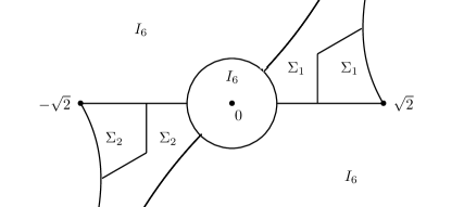
Figure 21. Constant matrix $M_{6}$

We arrive to the Riemann-Hilbert problem for $T(\lambda)=Z(\lambda)M_{6}$.

Riemann-Hilbert problem 3.11.

Consider the contour $\Gamma$ shown on Figure 22. The $6\times 6$ matrix valued function $T(\lambda)$ satisfies the following conditions

• $T(\lambda)$ is holomorphic on $\mathbb{C}\setminus\Gamma$.

• $T(\lambda)$ has finite boundary values on the contour $\Gamma$ and satisfies the jump condition indicated on Figure 22.

• $T(\lambda)$ has the asymptotic (3.15) at infinity and (3.16) at zero respectively.

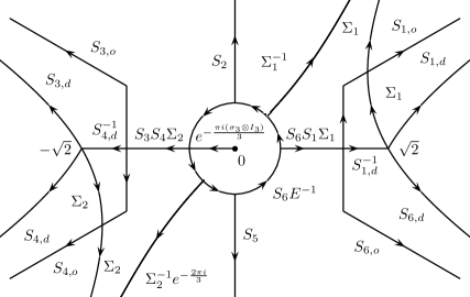
Figure 22. Contour for the Riemann-Hilbert problem 3.11

In particular we have the following products of matrices involved

$$S_{6}S_{1}\Sigma_{1}=\left(\begin{array}[]{cccccc}1&{b_{1}\sqrt{3}e^{\frac{5\pi i}{6}}{}}&{\sqrt{3}e^{\frac{2\pi i}{3}}{}}&-i&0&0\\ 0&1&0&0&e^{-\frac{\pi i}{6}}&0\\ 0&{\sqrt{3}e^{\frac{\pi i}{3}}{}}&1&0&0&e^{-\frac{5\pi i}{6}}\\ 0&{3i{}}&0&1&{b_{1}\sqrt{3}e^{\frac{i\pi}{6}}{}}&{\sqrt{3}e^{-\frac{2\pi i}{3}}{}}\\ 0&0&0&0&1&0\\ 0&-{3{}}&0&0&{\sqrt{3}e^{\frac{2\pi i}{3}}{}}&1\end{array}\right),$$

$$S_{3}S_{4}\Sigma_{2}=\left(\begin{array}[]{cccccc}1&{b_{1}\sqrt{3}e^{-\frac{5\pi i}{6}}{}}&{\sqrt{3}e^{\frac{i\pi}{3}}{}}&0&-{3i{}}&0\\ 0&1&0&0&0&0\\ 0&{\sqrt{3}e^{\frac{2\pi i}{3}}{}}&1&0&-{3{}}&0\\ -i&0&0&1&{b_{1}\sqrt{3}e^{-\frac{i\pi}{6}}{}}&{\sqrt{3}e^{-\frac{i\pi}{3}}{}}\\ 0&e^{-\frac{\pi i}{6}}&0&0&1&0\\ 0&0&e^{-\frac{5\pi i}{6}}&0&{\sqrt{3}e^{\frac{i\pi}{3}}{}}&1\end{array}\right).$$

We introduce notation for essential parts of these products

$$J_{1}=\left(\begin{array}[]{cccccc}1&0&0&0&0&0\\ 0&1&0&0&0&0\\ 0&0&1&0&0&0\\ 0&{3i{}}&0&1&0&0\\ 0&0&0&0&1&0\\ 0&-{3{}}&0&0&0&1\end{array}\right),$$

$$J_{2}=\left(\begin{array}[]{cccccc}1&0&0&0&-{3i{}}&0\\ 0&1&0&0&0&0\\ 0&0&1&0&-{3{}}&0\\ 0&0&0&1&0&0\\ 0&0&0&0&1&0\\ 0&0&0&0&0&1\end{array}\right).$$

Finally we perform the g-function transformation for this problem.

$$S(\lambda)=e^{(-t)^{\frac{3}{2}}(I_{2}\otimes\Lambda_{8})}(-t)^{-I_{2}\otimes\Lambda_{9}}T(\lambda)e^{(-t)^{\frac{3}{2}}g(\lambda)({\sigma}_{3}\otimes I_{3})}e^{-(-t)^{\frac{3}{2}}(I_{2}\otimes\Lambda_{8})}(-t)^{I_{2}\otimes\Lambda_{9}},$$

where

$$\Lambda_{8}=\dfrac{2\sqrt{2}}{3}\left(\begin{array}[]{ccc}-1&0&0\\ 0&1&0\\ 0&0&0\\ \end{array}\right),\quad\Lambda_{9}=\left(\begin{array}[]{ccc}\frac{17}{12}&0&0\\ 0&-\frac{13}{12}&0\\ 0&0&-\frac{1}{3}\end{array}\right).$$

Terms with $\Lambda_{9}$ will be used further in matching of parametrices.

We have the following sign charts describing behavior of $\mathrm{Re}\left(g(\lambda)\right)$.

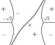
Figure 23. Sign chart for $\mathrm{Re}\left(g(\lambda)\right)$

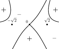
Figure 24. Sign chart for $\mathrm{Re}\left(g(\lambda)\right)+\frac{\sqrt{2}}{3}$

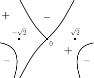
Figure 25. Sign chart for $\mathrm{Re}\left(g(\lambda)\right)-\frac{\sqrt{2}}{3}$

Similar to (3.6) we have

$$e^{-g({\sigma}_{3}\otimes I_{3})}e^{I_{2}\otimes\Lambda_{8}}\Upsilon e^{g({\sigma}_{3}\otimes I_{3})}e^{-I_{2}\otimes\Lambda_{8}}=\left(\begin{array}[]{cccccc}1&e^{-\frac{4\sqrt{2}}{3}}&e^{-\frac{2\sqrt{2}}{3}}&e^{-2g}&e^{-2g-\frac{4\sqrt{2}}{3}}&e^{-2g-\frac{2\sqrt{2}}{3}}\\ e^{\frac{4\sqrt{2}}{3}}&1&e^{\frac{2\sqrt{2}}{3}}&e^{-2g+\frac{4\sqrt{2}}{3}}&e^{-2g}&e^{-2g+\frac{2\sqrt{2}}{3}}\\ e^{\frac{2\sqrt{2}}{3}}&e^{-\frac{2\sqrt{2}}{3}}&1&e^{-2g+\frac{2\sqrt{2}}{3}}&e^{-2g-\frac{2\sqrt{2}}{3}}&e^{-2g}\\ e^{2g}&e^{2g-\frac{4\sqrt{2}}{3}}&e^{2g-\frac{2\sqrt{2}}{3}}&1&e^{-\frac{4\sqrt{2}}{3}}&e^{-\frac{2\sqrt{2}}{3}}\\ e^{2g+\frac{4\sqrt{2}}{3}}&e^{2g}&e^{2g+\frac{2\sqrt{2}}{3}}&e^{\frac{4\sqrt{2}}{3}}&1&e^{\frac{2\sqrt{2}}{3}}\\ e^{2g+\frac{2\sqrt{2}}{3}}&e^{2g-\frac{2\sqrt{2}}{3}}&e^{2g}&e^{\frac{2\sqrt{2}}{3}}&e^{-\frac{2\sqrt{2}}{3}}&1\end{array}\right)$$

We can see that after conjugation the jump matrices $S_{1,o},S_{3,o},S_{4,o},S_{6,o}$ are exponentially close to identity matrices. The products $S_{6}S_{1}\Sigma_{1}$ and $S_{3}S_{4}\Sigma_{1}$ after conjugation are exponentially close to $J_{1}$ and $J_{2}$. Conjugated jumps $S_{1,d},S_{2},S_{3,d},S_{4,d},S_{5},S_{6,d},J_{1},J_{2}$ are exponentially close to identity if you step away from points $\lambda=\pm\sqrt{2},0$. This outcome has motivated us to put offdiagonal elements of matrices $A,B,C$ to zero in (3.2).

As the result we have that $S(\lambda)$ has jumps exponentially close to identity everywhere except for neighborhoods of $\lambda=\pm\sqrt{2}$, $\lambda=0$ and parts with jumps $\Sigma_{1}$, $\Sigma_{2}$, $E^{-1}$. To cancel them we need to introduce parametrices solving the model Riemann-Hilbert problems.

3.2.2. Construction of parametrices

We start with global parametrix.

Riemann-Hilbert problem 3.12.

Consider the contour $\Gamma$ shown on Figure 26. The $6\times 6$ matrix valued function $P_{\infty}(\lambda)$ satisfies the following conditions

• $P_{\infty}(\lambda)$ is holomorphic on $\mathbb{C}\setminus\Gamma$.

• $P_{\infty}(\lambda)$ satisfies the jump condition indicated on Figure 26.

• $P_{\infty}(\lambda)$ has the asymptotic

  $$P_{\infty}(\lambda)=(I_{6}+O(\lambda^{-1}))\lambda^{I_{2}\otimes\Lambda},\quad\lambda\to\infty$$

  at infinity and satisfies the estimates

  $$P_{\infty}(\lambda)e^{-{i\pi}{}(\sigma_{3}\otimes\Lambda_{7})}(K\otimes I_{3})(\lambda-\sqrt{2})^{-\frac{1}{4}(\sigma_{3}\otimes I_{3})}=O(1),\quad\lambda\to\sqrt{2},$$

  $$P_{\infty}(\lambda)(\sigma_{3}\otimes I_{3})e^{{i\pi}{}(\sigma_{3}\otimes\Lambda_{7})}(K\otimes I_{3})(\lambda+\sqrt{2})^{\frac{1}{4}(\sigma_{3}\otimes I_{3})}=O(1),\quad\lambda\to-\sqrt{2},$$

  $$P_{\infty}(\lambda)=(K\otimes I_{3})e^{{i\pi}{}(\sigma_{3}\otimes\Lambda_{10})}2^{3{}(\sigma_{3}\otimes\Lambda_{10})}\lambda^{-2\sigma_{3}\otimes\Lambda_{10}+I_{2}\otimes\Lambda_{1}}(I_{6}+O(\lambda)),\quad\lambda\to 0,\quad\frac{\pi}{4}<\arg\lambda<\frac{5\pi}{4}$$

  $$P_{\infty}(\lambda)=(K\otimes I_{3})^{-1}e^{{i\pi}{}(\sigma_{3}\otimes\Lambda_{10})}2^{-3{}(\sigma_{3}\otimes\Lambda_{10})}\lambda^{2\sigma_{3}\otimes\Lambda_{10}+I_{2}\otimes\Lambda_{1}}(I_{6}+O(\lambda)),\quad\lambda\to 0,\quad-\frac{3\pi}{4}<\arg\lambda<\frac{\pi}{4}$$

  where

  $$\Lambda_{10}=\left(\begin{array}[]{ccc}\frac{1}{4}&0&0\\ 0&\dfrac{1}{12}&0\\ 0&0&\dfrac{5}{12}\\ \end{array}\right)=\Lambda_{7}+\frac{I_{3}}{4}.$$

Figure 26. Contour for the Riemann-Hilbert problem 3.12

The solution Riemann-Hilbert problem 3.12 can be constructed explicitly.

To describe the parametrix near $\lambda=\sqrt{2}$ we introduce

$$\frac{2}{3}\zeta^{\frac{3}{2}}=(-t)^{\frac{3}{2}}g(\lambda);\quad\zeta=(-t)\dfrac{1}{2^{\frac{4}{3}}}(2-\lambda^{2})\simeq(-t){2^{\frac{1}{6}}}e^{i\pi}(\lambda-\sqrt{2}),\quad\lambda\to\sqrt{2}$$

We will need solution to the following model Riemann-Hilbert problem

Riemann-Hilbert problem 3.13.

Consider the contour $\Gamma$ shown on Figure 27. It consists of rays starting at zero in directions $\arg(z)=0,\frac{2\pi}{3},\frac{4\pi}{3},-\frac{\pi}{3}$. The $6\times 6$ matrix valued function $\Phi_{\sqrt{2}}(z)$ satisfies the following conditions

• $\Phi_{\sqrt{2}}(z)$ is holomorphic on $\mathbb{C}\setminus\Gamma$.

• $\Phi_{\sqrt{2}}(z)$ has finite boundary values on contour $\Gamma$ and satisfies the jump condition indicated on Figure 27.

• $\Phi_{\sqrt{2}}(z)$ has the asymptotic

  $$\Phi_{\sqrt{2}}(z)=z^{-\frac{(\sigma_{3}\otimes I_{3})}{4}}(K\otimes I_{3})\left(I_{2}+O(z^{-1})\right)e^{-\frac{2}{3}{z^{\frac{3}{2}}}\sigma_{3}}e^{{i\pi}(\sigma_{3}\otimes\Lambda_{7})},\quad z\to\infty$$

  at infinity and satisfies the estimate $\Phi_{\sqrt{2}}(z)=O(1)$ at $z=0$.

Figure 27. Contour for the Riemann-Hilbert problem 3.13

The solution to Riemann-Hilbert problem 3.7 can be constructed using Airy functions. Using it we construct the parametrix near $\lambda=\sqrt{2}$.

$$P_{\sqrt{2}}=P_{\infty}e^{-{i\pi}(\sigma_{3}\otimes\Lambda_{7})}(K\otimes I_{3})^{-1}\zeta^{\frac{({\sigma}_{3}\otimes I_{3})}{4}}\Phi_{\sqrt{2}}(\zeta)e^{\frac{2}{3}\zeta^{\frac{3}{2}}({\sigma}_{3}\otimes I_{3})}$$

The cut for $\zeta^{\frac{1}{4}}$ is taken along $\gamma_{1}$. The expression $P_{\infty}e^{-{i\pi}(\sigma_{3}\otimes\Lambda_{7})}(K\otimes I_{3})^{-1}\zeta^{\frac{({\sigma}_{3}\otimes I_{3})}{4}}$ is holomorphic near $\lambda=\sqrt{2}$. The parametrix satisfies matching condition.

$$P_{\sqrt{2}}=P_{\infty}\left(I+O\left(\dfrac{1}{(-t)^{\frac{3}{2}}}\right)\right),\quad t\to-\infty$$ (3.17)

To describe the parametrix near $\lambda=-\sqrt{2}$ we introduce

$$\frac{2}{3}\zeta^{\frac{3}{2}}=-(-t)^{\frac{3}{2}}g(\lambda);\quad\zeta=(-t)\dfrac{1}{2^{\frac{4}{3}}}(2-\lambda^{2})\simeq(-t){2^{\frac{1}{6}}}(\lambda+\sqrt{2}),\quad\lambda\to-\sqrt{2}$$

We will need solution to the following model Riemann-Hilbert problem

Riemann-Hilbert problem 3.14.

Consider the contour $\Gamma$ shown on Figure 28. It consists of rays starting at zero in directions $\arg(z)=0,\frac{2\pi}{3},\frac{4\pi}{3},-\frac{\pi}{3}$. The $6\times 6$ matrix valued function $\Phi_{-\sqrt{2}}(z)$ satisfies the following conditions

• $\Phi_{-\sqrt{2}}(z)$ is holomorphic on $\mathbb{C}\setminus\Gamma$.

• $\Phi_{-\sqrt{2}}(z)$ has finite boundary values on contour $\Gamma$ and satisfies the jump condition indicated on Figure 28.

• $\Phi_{-\sqrt{2}}(z)$ has the asymptotic

  $$\Phi_{-\sqrt{2}}(z)=z^{-\frac{(\sigma_{3}\otimes I_{3})}{4}}(K\otimes I_{3})\left(I_{2}+O(z^{-1})\right)e^{-\frac{2}{3}{z^{\frac{3}{2}}}\sigma_{3}}e^{-{i\pi}(\sigma_{3}\otimes\Lambda_{7})}(\sigma_{1}\otimes I_{3}),\quad z\to\infty$$

  at infinity and satisfies the estimate $\Phi_{-\sqrt{2}}(z)=O(1)$ at $z=0$.

Figure 28. Contour for the Riemann-Hilbert problem 3.14

The solution to Riemann-Hilbert problem 3.7 can be constructed using Airy functions.

We construct the parametrix near $\lambda=-\sqrt{2}$

$$P_{-\sqrt{2}}=P_{\infty}e^{{i\pi}(\Lambda_{7}\otimes\sigma_{3})}(\sigma_{1}\otimes I_{3})(K\otimes I_{3})^{-1}\zeta^{\frac{({\sigma}_{3}\otimes I_{3})}{4}}(\Phi_{Airy}(\zeta)\otimes I_{3})e^{\frac{2}{3}\zeta^{\frac{3}{2}}({\sigma}_{3}\otimes I_{3})}$$

The cut for $\zeta^{\frac{1}{4}}$ is taken along $\gamma_{3}$. The expression $P_{\infty}e^{{i\pi}(\sigma_{3}\otimes\Lambda_{7})}(\sigma_{1}\otimes I_{3})(K\otimes\sigma_{3})^{-1}\zeta^{\frac{({\sigma}_{3}\otimes I_{3})}{4}}$ is holomorphic near $\lambda=-\sqrt{2}$. The parametrix satisfies matching condition.

$$P_{-\sqrt{2}}=P_{\infty}\left(I+O\left(\dfrac{1}{(-t)^{\frac{3}{2}}}\right)\right),\quad t\to-\infty$$ (3.18)

To describe the parametrix near $\lambda=0$ we introduce

$$\dfrac{\zeta^{2}}{4}=(-t)^{\frac{3}{2}}g(\lambda)\dfrac{\arg(\lambda-\sqrt{2})}{\pi}+(-t)^{\frac{3}{2}}\dfrac{\sqrt{2}}{3},\quad\zeta\simeq\lambda 2^{\frac{1}{4}}(-t)^{\frac{3}{4}},\quad\lambda\to 0.$$

We will need solution to the following model Riemann-Hilbert problem

Riemann-Hilbert problem 3.15.

Consider the contour $\Gamma$ shown on Figure 30. It consists of rays starting in directions $\arg(z)=0,\frac{\pi}{4},\frac{\pi}{2},{\pi}{},\frac{5\pi}{4},\frac{3\pi}{2}$ and a circle of fadius $\delta$. The $6\times 6$ matrix valued function $\Phi_{0}(z)$ satisfies the following conditions

• $\Phi_{0}(z)$ is holomorphic on $\mathbb{C}\setminus\Gamma$.

• $\Phi_{0}(z)$ has finite boundary values on contour $\Gamma$ and satisfies the jump condition indicated on Figure 30.

• $\Phi_{0}(z)$ has the asymptotic

  $$\Phi_{0}(z)=\left(I_{6}+\frac{m_{1,0}}{z}+O(z^{-2})\right)e^{\frac{z^{2}}{4}(\sigma_{3}\otimes I_{3})}z^{2(\sigma_{3}\otimes\Lambda_{10})+I_{2}\otimes\Lambda_{1}}M_{7}^{-1},\quad z\to\infty$$

  at infinity and satisfies the estimate $\Phi_{0}(z)z^{-\frac{1}{6}(\sigma_{3}\otimes I_{3})}=O(1)$ at $z=0$. The constant matrix $M_{7}$ is given by the Figure 29.

  

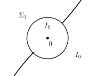
  Figure 29. Constant matrix $M_{7}$

Figure 30. Contour for the Riemann-Hilbert problem 3.15

The solution to Riemann-Hilbert problem 3.7 can be constructed using confluent hypergeometric functions. This construction allows us to evaluate

$$m_{1,0}=\left(\begin{array}[]{cccccc}0&0&0&0&0&0\\ 0&0&0&0&0&-\frac{i\Gamma\left(\frac{2}{3}\right)\Gamma\left(\frac{4}{3}\right)}{\pi}\\ 0&0&0&-\frac{{2^{\frac{2}{3}}{}e^{\frac{5\pi i}{6}}\Gamma\left(\frac{5}{3}\right)}}{\pi}&0&0\\ 0&0&\frac{{2^{\frac{2}{3}}{}e^{\frac{5\pi i}{6}}\Gamma\left(\frac{5}{3}\right)}}{\pi}&0&0&0\\ 0&0&0&0&0&0\\ 0&\frac{i\Gamma\left(\frac{2}{3}\right)\Gamma\left(\frac{4}{3}\right)}{\pi}&0&0&0&0\\ \end{array}\right)$$

We construct the parametrix near $\lambda=0$

$$P_{0}=A_{0}(\lambda)\Phi_{0}(\zeta(\lambda))e^{\frac{\arg(\lambda-\sqrt{2})}{i\pi}\frac{\zeta^{2}}{4}({\sigma}_{3}\otimes I_{3})}(-t)^{I_{2}\otimes\Lambda_{9}}$$

Here $A_{0}(\lambda)$ is the holomorphic function

$$A_{0}(\lambda)=P_{\infty}M_{7}\zeta^{-2\sigma_{3}\otimes\Lambda_{10}}\zeta^{-I_{2}\otimes\Lambda_{1}}(-t)^{-I_{2}\otimes\Lambda_{9}}=A_{0,0}+O(\lambda)$$

The matrix $A_{0,0}$ is given by

$$A_{0,0}=(K\otimes I_{3})^{-1}2^{-\frac{1}{4}(14\sigma_{3}\otimes\Lambda_{10}+I_{2}\otimes\Lambda_{1})}e^{i\pi\sigma_{3}\otimes\Lambda_{10}}(-t)^{-\frac{1}{4}(6\sigma_{3}\otimes\Lambda_{10}+3I_{2}\otimes\Lambda_{1}+4I_{2}\otimes\Lambda_{9})}.$$

We have the matching condition

$$P_{0}=P_{\infty}\left(I+O\left(\dfrac{1}{(-t)^{\frac{3}{4}}}\right)\right)$$ (3.19)

3.2.3. Computation of asymptotic

Now, having all parametrices constructed we define

$$S_{as}=\left\{\begin{array}[]{cc}P_{0},&\quad|\lambda|<\delta,\\ P_{\sqrt{2}},&\quad|\lambda-\sqrt{2}|<\delta,\\ P_{-\sqrt{2}},&\quad|\lambda+\sqrt{2}|<\delta,\\ P_{\infty},&\quad\mbox{otherwise}.\end{array}\right.$$

for small number $\delta$. Then we arrive to the Riemann Hilbert problem for $R=SS_{as}^{-1}$ with small jump.

Riemann-Hilbert problem 3.16.

Consider the contour $\Gamma$ shown on Figure 31. The $6\times 6$ matrix valued function $R(\lambda)$ satisfies the following conditions

• $R(\lambda)$ is holomorphic on $\mathbb{C}\setminus\Gamma$.

• $R(\lambda)$ has finite boundary values on the contour $\Gamma$ and satisfies the jump condition indicated on Figure 31. On the non-labeled parts of contour the jump is obtained from the jump for $S(\lambda)$ conjugating with $S_{as}(\lambda)$.

• $R(\lambda)$ has the asymptotic at infinity

  $$R(\lambda)=I_{6}+\frac{l_{1}}{\lambda}+O(\lambda^{-2}),\quad\lambda\to\infty$$

  .

Figure 31. Contour for the Riemann-Hilbert problem 3.16

We have again $P_{\infty}(\lambda)$ growing at infinity and we can do the estimates similar to (3.10). After that, using (3.17), (3.18),(3.19) we get

$$|J(\mu)-I_{6}|=O((-t)^{-\frac{3}{4}}).$$ (3.20)

Now following the standard procedure we write the singular integral equation for $R_{-}(\lambda)$.

$$R_{-}(\lambda)=I-\intop_{\Gamma}\frac{R_{-}(\mu)(J(\mu)-1)}{\mu-\lambda+i0}\frac{d\mu}{2\pi i},$$

where $J(\lambda)$ is the jump matrix. Using (3.20) we get

$$R(\lambda)=I+O((-t)^{-\frac{3}{4}}).$$ (3.21)

We also have the formula for $R(\lambda)$ away from contour $\Gamma$.

$$R(\lambda)=I-\intop_{\Gamma}\frac{R_{-}(\mu)(J(\mu)-1)}{\mu-\lambda}\frac{d\mu}{2\pi i}$$

Expanding it at infinity we get

$$l_{1}=\intop_{\Gamma}{R_{-}(\mu)(J(\mu)-1)}\frac{d\mu}{2\pi i}.$$

Using the estimates (3.21), (3.20) we arrive at

$$l_{1}=\intop_{\Gamma}{(J(\mu)-1)}\frac{d\mu}{2\pi i}+O((-t)^{-\frac{3}{2}}).$$

The main part of this integral comes from circle around $\lambda=0$.

$$l_{1}=\intop_{|\mu|=\delta}{(J(\mu)-1)}\frac{d\mu}{2\pi i}+O((-t)^{-\frac{3}{2}}).$$

Using the expansion for $\Phi_{0}$ at infinity we get

$$l_{1}=-\dfrac{A_{0,0}m_{1,0}A_{0,0}^{-1}}{{2^{\frac{1}{4}}}(-t)^{\frac{3}{4}}}+O((-t)^{-\frac{3}{2}}).$$

Tracing back the transformations from section 3.1.1 we have

$$m_{1}=\sqrt{-t}P_{1}e^{-(I_{2}\otimes\Lambda_{8})(-t)^{\frac{3}{2}}}(-t)^{I_{2}\otimes\Lambda_{9}+\frac{1}{2}I_{2}\otimes\Lambda_{1}}\left(\frac{\sigma_{2}\otimes I_{3}}{\sqrt{2}}+l_{1}\right)e^{(I_{2}\otimes\Lambda_{8})(-t)^{\frac{3}{2}}}t^{-I_{2}\otimes\Lambda_{9}-\frac{1}{2}I_{2}\otimes\Lambda_{1}}P_{1}^{-1}.$$

Using the formula $q(t)=-i\hat{m}_{1,12}$ we have

$$\det(q(t)-xI_{3})=-x^{3}+\left(-3\sqrt{\frac{-t}{2}}+O(t^{-1})\right)x^{2}+\left(\frac{3t}{2}+O((-t)^{-\frac{1}{2}})\right)x-\left(\frac{-t}{2}\right)^{\frac{3}{2}}+O(1).$$

Using Cardano formula we have the following asymptotic of eigenvalues up to permutation

$$x_{1}=-\sqrt{\frac{-t}{2}}+O(t^{-1}),\quad x_{2}=-\sqrt{\frac{-t}{2}}+\frac{i}{{2^{\frac{3}{4}}(-t)^{\frac{1}{4}}}}+O(t^{-1}),\quad x_{3}=-\sqrt{\frac{-t}{2}}-\frac{i}{{2^{\frac{3}{4}}(-t)^{\frac{1}{4}}}}+O(t^{-1})$$

The asymptotic of solutions have form

$$x_{1}=-\sqrt{\frac{-t}{2}}+\sum_{j=0}^{\infty}c_{j}(-t)^{-1-\frac{3}{4}j},\quad x_{2}=-\sqrt{\frac{-t}{2}}+\frac{i}{{2^{\frac{3}{4}}(-t)^{\frac{1}{4}}}}+\sum_{j=0}^{\infty}d_{j}(-t)^{-1-\frac{3}{4}j},\quad x_{3}=-\sqrt{\frac{-t}{2}}-\frac{i}{{2^{\frac{3}{4}}(-t)^{\frac{1}{4}}}}+\sum_{j=0}^{\infty}e_{j}(-t)^{-1-\frac{3}{4}j},$$

We rewrite the Calogero-Painlevé system in the following form

$$\begin{gathered}3(x_{1}-x_{2})^{3}(x_{1}-x_{3})^{3}(-6x_{1}^{\prime\prime}+12x_{1}^{3}+6x_{1}t-1)-4((x_{1}-x_{2})^{3}+(x_{1}-x_{3})^{3})=0\\ 3(x_{2}-x_{3})^{3}(x_{2}-x_{1})^{3}(-6x_{2}^{\prime\prime}+12x_{2}^{3}+6x_{2}t-1)-4((x_{2}-x_{1})^{3}+(x_{2}-x_{3})^{3})=0\\ 3(x_{3}-x_{2})^{3}(x_{3}-x_{1})^{3}(-6x_{3}^{\prime\prime}+12x_{3}^{3}+6x_{3}t-1)-4((x_{3}-x_{2})^{3}+(x_{3}-x_{1})^{3})=0\end{gathered}$$ (3.22)

We have

$$(x_{1}-x_{2})^{3}=\frac{i}{2^{\frac{9}{4}}(-t)^{\frac{3}{4}}}-\frac{3}{2\sqrt{2}}\sum_{k=2}^{\infty}(c_{k-2}-d_{k-2})(-t)^{-\frac{3}{4}k}-\frac{3i}{2^{\frac{3}{4}}}\sum_{k=3}^{\infty}\sum_{j=0}^{k-3}(c_{j}-d_{j})(c_{k-j-3}-d_{k-j-3})(-t)^{-\frac{3}{4}k}$$

$$+\sum_{k=4}^{\infty}\sum_{j_{1}=0}^{k-4}\sum_{j_{2}=0}^{k-4-j_{1}}(c_{j_{1}}-d_{j_{1}})(c_{j_{2}}-d_{j_{2}})(c_{k-4-j_{1}-j_{2}}-d_{k-4-j_{1}-j_{2}})(-t)^{-\frac{3}{4}k}$$

$$(x_{1}-x_{3})^{3}=-\frac{i}{2^{\frac{9}{4}}(-t)^{\frac{3}{4}}}-\frac{3}{2\sqrt{2}}\sum_{k=2}^{\infty}(c_{k-2}-e_{k-2})(-t)^{-\frac{3}{4}k}+\frac{3i}{{2^{\frac{3}{4}}}}\sum_{k=3}^{\infty}\sum_{j=0}^{k-3}(c_{j}-e_{j})(c_{k-j-3}-e_{k-j-3})(-t)^{-\frac{3}{4}k}$$

$$+\sum_{k=4}^{\infty}\sum_{j_{1}=0}^{k-4}\sum_{j_{2}=0}^{k-4-j_{1}}(c_{j_{1}}-e_{j_{1}})(c_{j_{2}}-e_{j_{2}})(c_{k-4-j_{1}-j_{2}}-e_{k-4-j_{1}-j_{2}})(-t)^{-\frac{3}{4}k}$$

$$(x_{2}-x_{3})^{3}=-\frac{i2^{\frac{3}{4}}}{(-t)^{\frac{3}{4}}}-3\sqrt{2}\sum_{k=2}^{\infty}(d_{k-2}-e_{k-2})(-t)^{-\frac{3}{4}k}+{3i2^{\frac{1}{4}}}{}\sum_{k=3}^{\infty}\sum_{j=0}^{k-3}(d_{j}-e_{j})(d_{k-j-3}-e_{k-j-3})(-t)^{-\frac{3}{4}k}$$

$$+\sum_{k=4}^{\infty}\sum_{j_{1}=0}^{k-4}\sum_{j_{2}=0}^{k-4-j_{1}}(d_{j_{1}}-e_{j_{1}})(d_{j_{2}}-e_{j_{2}})(d_{k-4-j_{1}-j_{2}}-d_{k-4-j_{1}-j_{2}})(-t)^{-\frac{3}{4}k}$$

$$x_{1}^{\prime\prime}=\frac{1}{4\sqrt{2}{(-t)^{\frac{3}{2}}}}+\sum_{k=4}^{\infty}\left(2-\frac{3}{4}k\right)\left(1-\frac{3}{4}k\right)c_{k-4}t^{-\frac{3}{4}k}$$

$$x_{2}^{\prime\prime}=\frac{1}{4\sqrt{2}{(-t)^{\frac{3}{2}}}}+\frac{5i}{2^{\frac{3}{4}}16(-t)^{-\frac{9}{4}}}+\sum_{k=4}^{\infty}\left(2-\frac{3}{4}k\right)\left(1-\frac{3}{4}k\right)d_{k-4}t^{-\frac{3}{4}k}$$

$$x_{3}^{\prime\prime}=\frac{1}{4\sqrt{2}{(-t)^{\frac{3}{2}}}}-\frac{5i}{2^{\frac{3}{4}}16(-t)^{-\frac{9}{4}}}+\sum_{k=4}^{\infty}\left(2-\frac{3}{4}k\right)\left(1-\frac{3}{4}k\right)e_{k-4}t^{-\frac{3}{4}k}$$

$$x_{1}^{3}=-\frac{(-t)^{\frac{3}{2}}}{2\sqrt{2}}+\frac{3}{2}\sum_{k=0}^{\infty}c_{k}t^{-\frac{3}{4}k}-\frac{3}{\sqrt{2}}\sum_{k=2}^{\infty}\sum_{j=0}^{k-2}c_{j}c_{k-j-2}t^{-\frac{3}{4}k}$$

$$+\sum_{k=4}^{\infty}\sum_{j_{1}=0}^{k-4}\sum_{j_{2}=0}^{k-4-j_{1}}c_{j_{1}}c_{j_{2}}c_{k-4-j_{1}-j_{2}}t^{-\frac{3}{4}k}$$

$$x_{2}^{3}=-\frac{(-t)^{\frac{3}{2}}}{2\sqrt{2}}+\frac{3i(-t)^{\frac{3}{4}}}{2^{\frac{7}{4}}}+\frac{3}{2}\sum_{k=0}^{\infty}d_{k}t^{-\frac{3}{4}k}+\frac{3}{4}-\frac{3i}{2^{\frac{1}{4}}}\sum_{k=1}^{\infty}d_{k-1}t^{-\frac{3}{4}k}-\frac{3}{\sqrt{2}}\sum_{k=2}^{\infty}\sum_{j=0}^{k-2}d_{j}d_{k-j-2}t^{-\frac{3}{4}k}-\frac{i}{2^{\frac{9}{4}}(-t)^{\frac{3}{4}}}$$

$$-\frac{3}{2\sqrt{2}}\sum_{k=2}^{\infty}d_{k-2}(-t)^{-\frac{3}{4}k}+\frac{3i}{{2^{\frac{3}{4}}}}\sum_{k=3}^{\infty}\sum_{j=0}^{k-3}d_{j}d_{k-j-3}(-t)^{-\frac{3}{4}k}+\sum_{k=4}^{\infty}\sum_{j_{1}=0}^{k-4}\sum_{j_{2}=0}^{k-4-j_{1}}d_{j_{1}}d_{j_{2}}d_{k-4-j_{1}-j_{2}}(-t)^{-\frac{3}{4}k}$$

$$x_{3}^{3}=-\frac{(-t)^{\frac{3}{2}}}{2\sqrt{2}}-\frac{3i(-t)^{\frac{3}{4}}}{2^{\frac{7}{4}}}+\frac{3}{2}\sum_{k=0}^{\infty}e_{k}t^{-\frac{3}{4}k}+\frac{3}{4}+\frac{3i}{2^{\frac{1}{4}}}\sum_{k=1}^{\infty}e_{k-1}t^{-\frac{3}{4}k}-\frac{3}{\sqrt{2}}\sum_{k=2}^{\infty}\sum_{j=0}^{k-2}e_{j}e_{k-j-2}t^{-\frac{3}{4}k}+\frac{i}{2^{\frac{9}{4}}(-t)^{\frac{3}{4}}}$$

$$-\frac{3}{2\sqrt{2}}\sum_{k=2}^{\infty}e_{k-2}(-t)^{-\frac{3}{4}k}-\frac{3i}{{2^{\frac{3}{4}}}}\sum_{k=3}^{\infty}\sum_{j=0}^{k-3}e_{j}e_{k-j-3}(-t)^{-\frac{3}{4}k}+\sum_{k=4}^{\infty}\sum_{j_{1}=0}^{k-4}\sum_{j_{2}=0}^{k-4-j_{1}}e_{j_{1}}e_{j_{2}}e_{k-4-j_{1}-j_{2}}(-t)^{-\frac{3}{4}k}$$

We can see that in (3.22) in the coefficient near $t^{-\frac{3}{4}k}$ the terms with highest indices $c_{k-2},d_{k-2},e_{k-2}$ come from the terms

$$\begin{gathered}18(x_{1}-x_{2})^{3}(x_{1}-x_{3})^{3}(2x_{1}^{3}+x_{1}t)-4((x_{1}-x_{2})^{3}+(x_{1}-x_{3})^{3}),\\ 18(x_{2}-x_{3})^{3}(x_{2}-x_{1})^{3}(2x_{2}^{3}+x_{2}t)-4((x_{2}-x_{1})^{3}+(x_{2}-x_{3})^{3}),\\ 18(x_{3}-x_{2})^{3}(x_{3}-x_{1})^{3}(2x_{3}^{3}+x_{3}t)-4((x_{3}-x_{2})^{3}+(x_{3}-x_{1})^{3}),\end{gathered}$$ (3.23)

It has form

$$\left(\begin{array}[]{ccc}\frac{57\sqrt{2}}{8}&-3\sqrt{2}&-3\sqrt{2}\\ 24\sqrt{2}&-\frac{69\sqrt{2}}{2}&\frac{3\sqrt{2}}{{2}}\\ 24\sqrt{2}&\frac{3\sqrt{2}}{{2}}&-\frac{69\sqrt{2}}{2}\end{array}\right)\left(\begin{array}[]{c}c_{k-2}\\ d_{k-2}\\ e_{k-2}\end{array}\right)+\mbox{lower terms}$$

The determinant of the matrix above is $6561\sqrt{2}$, so we derived the recurrence relation for the coefficients $c_{k},e_{k},d_{k}$. We don’t write the explicit formula for it. It determines all the coefficients uniquely.

References

- [BBDiF] J. Baik, R. Buckingham, and J. DiFranco, Asymptotics of Tracy-Widom distributions and the total integral of a Painlevé II function, Commun. Math. Phys. 280 (2008), 463Ð497.arXiv:math.FA/0704.3636v1 (2007).
- [BCR] M. Bertola, M. Cafasso, V. Roubtsov, Noncommutative Painlevé equations and systems of Calogero type, Commun. Math. Phys. 363 (2018), arXiv:1710.00736 [math-ph].
- [BV] A. Bloemendal, B. Virág, Limits of spiked random matrices I. Probab. Theory Related Fields156 (2013), no. 3-4, 795 - 825, arXiv:1011.1877.
- [BO] A. Borodin, G. Olshanski, Z-measures on partitions and their scaling limits. European Journal of Combinatorics, 6, no. 26, (2015), 795-834;
- [BEMN] G. Borot, B. Eynard, S. N. Majumdar, C. Nadal, Large deviations of the maximal eigenvalue of random matrices. J. Stat. Mech. Theory Exp. 11 (2011), P11024, 56 pp. arXiv:1009.1945.
- [BN] G. Borot, C. Nadal, Right tail asymptotic expansion of Tracy-Widom beta laws, Random Matrices: Theory and Applications, Vol. 01, No. 03, 1250006 (2012).
- [EGO] P. Etingof, W. L. Gan, A. Oblomkov, Generalized double affine Hecke algebras of higher rank, Journal fur die reine und angewandte Mathematic, 2006, 600, DOI: 10.1515/CRELLE.2006.091 , arXiv: math/0504089
- [DIK] P. Deift, A. Its, I. Krasovsky, Asymptotics of the Airy-kernel determinant, Comm. Math. Phys. 278, no. 3, (2008), 643-678; arXiv:math/0609451 [math.FA].
- [DE] I. Dumitriu, A. Edelman , Matrix models for beta ensembles. J. Math. Phys. 43 (2002), 5830 - 5847.
- [FIKN] A. Fokas, A. Its, A. Kapaev, V. Novokshenov, Painlev´e transcendents. The Riemann-Hilbert Approach, AMS Series: Mathematical Surveys and Monographs, vol. 128, 2006.
- [For] P. Forrester, Asymptotics of spacing distributions 50 years later, in Random matrix theory, interacting particle systems, and integrable systems, 199 - 222, Math. Sci. Res. Inst. Publ., 65, Cambridge Univ. Press, New York, 2014, arXiv:1204.3225.
- [For2] P. Forrester, Log-Gases and Random Matrices, London Mathematical Society Monographs Series, v. 34, Princeton University Press. 2010.
- [GIKM] T. Grava, A. Its, A. Kapaev, F. Mezzadri, On the Tracy-Widomβ distribution fro , SIGMA, 12, 2016, 26 pages, arXiv: 1607.01351v1
- [GH] A. Guionnet, J. Huang, Rigidity and Edge Universality of Discrete -Ensembles , Communications on pure and applied mathematics, Vol. 72, Issue 9, (2019).
- [Ino] V. I. Inozemtsev, Lax representation with spectral parameter on a torus for integrable particle systems. Lett. Math. Phys., 17:11-17, 1989.
- [L] Y. Li, On the Open Question of The Tracy-Widom Distribution of -Ensemble With , arXiv:1812.00522 [math-ph].
- [RRV] J. A. Ramírez, B. Rider, B, Virág, Beta ensembles, stochastic Airy spectrum, and a diffusion, J. Amer. Math. Soc., 24 (2011), no. 4, 919 - 944, arXiv:math/0607331.
- [Rum1] I. Rumanov, Classical integrability for beta-ensembles and general Fokker-Plank equations, J. Math. Phys., 56 (2015), no. 1 013508, 16pp, arXiv:1306.2117.
- [Rum2] I. Rumanov, Painlevé Representation of distribution for = 6, Comm. Math. Phys. 342 (2016), no. 3, 843 - 868.
- [Rum3] I. Rumanov, Beta ensembles, quantum Painlevé equations and isomonodromy systems, Contemp. Math. AMS series, v. 651 (2015), pp. 125 -155, arXiv:1408.3847.
- [Tak] K. Takasaki, Painlevé-Calogero correspondence revisited. J. Math. Phys., 42(3):1443-1473, 2001.
- [TW] C. A. Tracy, H. Widom, Level-spacing distributions and the Airy kernel, Comm. Math. Phys. 159, (1994), 151-174; hep-th/9211141.
- [VV] B. Valkó, B. Virág, Continuum limits of random matrices and the Brownian carousel. Invent. Math. 177 (2009), no. 3, 463 - 508. arXiv:0712.2000