Downscale energy fluxes in scale invariant
oceanic internal wave turbulence

Abstract

We analyze analytically and numerically the scale invariant stationary solution to the internal wave kinetic equation. Our analysis of the resonant energy transfers shows that the leading order contributions are given (i) by triads with extreme scale separation and (ii) by triads of waves that are quasi-colinear in the horizontal plane. The contributions from other types of triads is found to be subleading. We use the modified scale invariant limit of the Garrett and Munk spectrum of internal waves to calculate the magnitude of the energy flux towards high wave numbers in both the vertical and the horizontal directions. Our results compare favorably with the finescale parametrization of ocean mixing that was proposed in [Polzin et al. (1995)].

1 Introduction

Internal waves are the gravity waves that oscillate in the bulk of the stratified ocean due to the modulation of surfaces of constant density. Internal waves are ubiquitous in the ocean, contain a large amount of energy, and affect significantly the processes involved in water mixing and transport. Understanding the role played by internal gravity waves in the energy budget of the oceans represents a major challenge in physical oceanography, intimately related to the quantification of ocean mixing [Ferrari & Wunsch (2008); Polzin et al. (2014)]. Internal waves constitute a highly complex problem, involving scales from few meters to hundreds of kilometers, and periods ranging from a few minutes up to days. The processes that supply energy to and remove energy from internal waves include interactions with surface gravity waves, mesoscale eddies, scattering of the tidal flow from the bottom topography, overturning of wave fronts and wave breaking. These pumping and damping processes are characterized by vastly different spatial and temporal scales. Despite this enormous complexity, the spectral energy density of internal waves is thought to be pretty universal, and is given by what is now called Garrett and Munk spectrum of internal waves. First proposed in 1972 [Garrett & Munk (1972)], then subject to subsequent revisions, [Garrett & Munk (1975); Cairns & Williams (1976); Garrett & Munk (1979)], the Garrett and Munk spectrum (GM, from now on referring to the 1976 version) has since become the accepted default choice to quantify the oceanic internal wave field. Since then substantial deviations, both seasonal and regional, were documented (notably near boundaries, [Wunsch & Webb (1979); Polzin (2004); Polzin & Lvov (2011)], and at the equator, [Eriksen (1985)]). Nonetheless, the GM spectrum has survived to our day as the standard for inter-comparison of different data sets, to the amazement of Chris Garrett and Walter Munk themselves [von Storch & Hasselmann (2010)], providing the baseline for generalizations that try to account for the observed variability [Polzin & Lvov (2011)].

The spectral energy fluxes in the oceanic internal wave field have been a subject of intense investigation in the last four decades [Müller et al. (1986); McComas & Bretherton (1977); Olbers (1973); Polzin et al. (1995)]. Understanding these energy fluxes is crucial for climate modeling and predictions, since internal waves are not resolved in Global Circulation Models (GCM) and they are replaced by simple phenomenological formulas [MacKinnon et al. (2017)] . One of such broadly used expressions is the finescale parametrization formula derived in [Polzin et al. (1995)].

In this paper we use the wave turbulence theory for internal gravity waves developed in [Lvov & Tabak (2001, 2004); Lvov et al. (2010); Lvov & Yokoyama (2009)] and reviewed in [Polzin & Lvov (2011)] to analyze these energy fluxes towards high wave numbers. We assume that the spectral energy density of internal waves is given by a simple scale invariant solution, that was found in [Lvov et al. (2010)], (hereafter, the convergent stationary solution of the internal wave kinetic equation, Eq. (17) in the body of the paper). Interestingly, this scale invariant spectrum is close to the scale invariant limit of the famous Garrett and Munk (GM) spectrum of internal waves [Garrett & Munk (1972); Cairns & Williams (1976); Garrett & Munk (1979)], see Eq. (3) in the body of the paper. Thus, slightly adjusting the GM spectrum so that its scale invariant limit matches the power-law behavior of the convergent stationary solution, we compute the energy flux via the collision integral of the wave kinetic equation. This collision integral contains complete information concerning resonant spectral energy transfers. The computation of the flux is performed numerically. Our expression for these energy fluxes compares favorably with the finescale parametrization formula put forward in [Polzin et al. (1995)].

To characterize the energy fluxes towards high wave numbers we investigate the formation of the stationary wave spectra in the kinetic equation. We therefore analyze and classify the contributions of the various resonant triads that contribute to the kinetic equation. The importance of triads with extreme scale separation were previously identified in the literature [McComas & Bretherton (1977)] and named Induced Diffusion (ID), Parametric Subharmonic Instability (PSI) and Elastic Scattering (ES). In addition, we point out an additional class of important interactions that are colinear, or almost so, in the horizontal plane, which appear to contribute significantly to the formation of the stationary state and the fluxes of energy.

The paper is written as follows. In Section 2 we give the reader the relevant background along with necessarily brief literature review. In Section 3 we analyze the convergence conditions of the collision integral at the infrared and the ultraviolet limits. We perform a rigorous numerical integration paying special attention to accurately integrate integrable singularities of the kinetic equation kernel. We also analyze in details the nature of the interacting triads contributing to the stationary scale invariant solution of the kinetic equation. An analytical and numerical analysis of these various contributions is presented in Section 4, highlighting the main physical mechanisms at play. In Section 5 we compute the energy fluxes toward the small scales and thereby quantify the total dissipated energy. Finally, we summarize our results in Section 6.

2 Background material

2.1 Internal waves and the Garrett and Munk spectrum

Garrett and Munk have observed that the internal wave spectrum is separable in frequency-vertical wave numbers. In other words it can be accurately represented as a product of a function of frequency and a function of vertical wave number. The GM energy spectrum is therefore represented in the two-dimensional domain of vertical wavenumber $m$ with $m\in[m_{\min},m_{\max}]$ and frequency $\sigma$ with $\sigma\in[f,N]$ as

$$\qquad e_{\rm GM}(m,\sigma)=N_{0}Nb^{2}EA(m)B(\sigma)\,,$$ (1)

$$A(m)=\frac{2}{\pi}\frac{m_{\star}}{m_{\star}^{2}+m^{2}}\,,\qquad B(\sigma)=\frac{2f}{\pi}\frac{1}{\sigma\sqrt{\sigma^{2}-f^{2}}}\,,\qquad m_{\star}=\frac{3\pi}{b}{\color[rgb]{0,0,0}\frac{N}{N_{0}}}\,,$$ (2)

normalized in such a way that $\int_{m_{\min}}^{m_{\max}}A(m)dm\simeq\int_{0}^{\infty}A(m)dm=1$, $\int_{f}^{N}B(\sigma)d\sigma\simeq\int_{0}^{\infty}B(\sigma)d\sigma=1$, and the total energy density (per unit mass) is therefore given by $N_{0}Nb^{2}E$, in units of ${\rm J}\,{\rm kg}^{-1}$. Here $N$ and $N_{0}=0.00524\;{\rm s}^{-1}$ are respectively the buoyancy frequency and the reference buoyancy frequency, $f=2\times 7.3\times 10^{-5}\sin(l)\;{\rm s}^{-1}$ is the Coriolis parameter computed at latitude $l=32.5^{\circ}$, $b=1300\;{\rm m}$ is the scale height of the ocean, $E=6.3\times 10^{-5}$ is the GM specification of the nondimensional energy level, and $m_{\star}$ is a reference vertical wave number. Furthermore, $m_{\rm min}=2\pi(2600\text{ m})^{-1}\,,$ $m_{\rm max}=2\pi(10\text{ m})^{-1}$ are the physical cutoffs imposed by the ocean depth and by wave breaking, respectively.

2.2 Wave-turbulence interpretation of the GM spectrum

Despite the GM far reaching combination of simplicity and descriptive power of available field measurements, its phenomenological nature does not necessarily provide an explanation to the underlying physics. Since the 1970s, the concept of nonlinear interactions has become the leit motiv in the search for a physical interpretation of the GM spectrum starting from the primitive equations of a stratified ocean, [McComas & Bretherton (1977); McComas & Müller (1981); Holloway et al. (1986); Müller et al. (1986); Olbers (1973, 1976); Pelinovsky & Raevsky (1977); Caillol & Zeitlin (2000); Voronovich (1979); Lvov & Tabak (2001)]. The quadratic nonlinearity in the primitive fluid equations and a dispersion relation allowing for three-wave interactions imply that internal waves interact through triads. In a weakly nonlinear regime, three-wave resonant interactions are responsible for slow, net energy transfers between different wave numbers, [Davis et al. (2020)]. This process can be described by a wave kinetic equation, the evolution equation of the action spectrum of the internal wavefield, [Hasselmann (1966); Zakharov et al. (1992); Nazarenko (2011)]. In the present paper we use the three-dimensional wave number domain $\mathbf{p}=(\mathbf{k},m)$, where $\mathbf{k}$ and $m$ are the horizontal and the vertical wave numbers, respectively. Note that $\mathbf{k}$ is a two-dimensional horizontal wave vector and we define its norm as $k:=|\mathbf{k}|$. The dispersion relation of internal gravity waves is given by $\sigma^{2}_{\bf p}=f^{2}+N^{2}\frac{k^{2}}{m^{2}}$. which can be used to switch from one domain to the other, since only two of the three variables $k$, $m$ and $\sigma$ are independent. The action spectrum is related to the energy spectrum (now both intended as three-dimensional spectra) via $e(\mathbf{k},m)=\sigma n(\mathbf{k},m)$, where for simplicity we use the quantities in brackets to specify the domain of dependence of the quantity of interest. We assume horizontal and vertical isotropy, so that we have $e(m,\sigma)={\color[rgb]{0,0,0}4}\pi ke(\mathbf{k},m)\left(\frac{d\sigma}{dk}\right)^{-1}$, after integrating over the horizontal azimuthal angle and considering a positive definite $m$. Considering the scale invariant (or non-rotating) limit $f\ll\sigma\ll N$, which yields the scale-invariant dispersion relation (here defined as the positive branch) $\sigma=Nk/|m|\,$, Eq. 1 transforms into

$$n_{\rm GM}(\mathbf{k},m)=\frac{{\color[rgb]{0,0,0}1}}{\pi^{3}}\frac{Eb^{2}{\color[rgb]{0,0,0}N_{0}}fm_{\star}}{{\color[rgb]{0,0,0}N}}k^{-4}\,,$$ (3)

which represents the non-rotating limit of the GM three-dimensional action spectrum, in the horizontal wave number - vertical wave number domain.

The wave turbulence theory for internal waves was revisited with the generalized random phase and amplitude formalism ([Choi et al. (2004, 2005); Nazarenko (2011)]) in the series of works [Lvov & Tabak (2001); Lvov et al. (2004, 2010)], where the internal wave kinetic equation was derived starting from the primitive equations of motion in hydrostatic balance by using isopycnal coordinates. A detailed review is found in the introductory paragraphs of [Lvov et al. (2010)], and will not be repeated here. The main steps can be schematized as follows: (i) The primitive equations of a vertically stratified ocean in hydrostatic balance and with no background rotation are rewritten in isopycnal coordinates under the Boussinesq approximation. The scale invariant limit of the dispersion relation in the new variables reads (with no background rotation)

$$\sigma(\mathbf{k},m)=\frac{g}{\rho_{0}N}\frac{k}{|m|}\,,$$ (4)

where $g$ is the acceleration of gravity, $\rho_{0}$ is the reference density and the vertical wave number $m$ is now an inverse density. (ii) In the isopycnal formulation the equations of motion are reduced to Hamiltonian form for the two conjugate fields $\phi$ and $\Pi$, the velocity potential and the normalized differential layer thickness. (iii) The machinery of wave turbulence is applied by switching to Fourier space and introducing the complex canonical normal variables $c_{\mathbf{p}}$ and $c_{-\mathbf{p}}^{*}$, representing complex amplitudes of the normal modes of the system. Under the assumption of spatial homogeneity, the action spectral density is defined as

$$\langle c_{\mathbf{p}_{1}}c_{\mathbf{p}_{2}}^{*}\rangle=n_{\mathbf{p}_{1}}\delta_{\mathbf{p}_{1}-\mathbf{p}_{2}}\,,$$ (5)

where $\delta(\cdot)$ is a Dirac delta, and the angular brackets denote averaging on a suitably defined statistical ensemble: under the standard assumptions of random phases and amplitudes [Zakharov et al. (1992); Nazarenko (2011)], in the joint limit of large box and small nonlinearity the following wave kinetic equation is derived, assuming isotropy in the horizontal plane (for simplicity, here written in the non-rotating limit:

$$\frac{\partial n_{\mathbf{p}}}{\partial t}=\frac{8\pi}{k}\int\left(f^{\mathbf{p}}_{12}|V^{\mathbf{p}}_{12}|^{2}\delta_{m-m_{1}-m_{2}}\delta_{\sigma_{\mathbf{p}}-\sigma_{1}-\sigma_{2}}\frac{kk_{1}k_{2}}{\Delta_{\mathbf{p}12}}-(0\leftrightarrow 1)-(0\leftrightarrow 2)\right)dk_{1}dk_{2}dm_{1}dm_{2}\,,$$ (6)

where $n_{\mathbf{p}}=n(\mathbf{k},m;t)$ is the three-dimensional action spectrum defined in (5), $f^{\mathbf{p}}_{12}=n_{1}n_{2}-n_{\mathbf{p}}(n_{1}+n_{2})$, $V^{\mathbf{p}}_{12}$ is the matrix element describing the magnitude of nonlinear interactions between the triad of wave numbers $\mathbf{p}$, $\mathbf{p}_{1}$ and $\mathbf{p}_{2}$, given below by (11). Furthermore the two delta functions impose the conservation of vertical momentum and energy in each three-wave interaction. The $\Delta_{\mathbf{p}12}$, given by (10), is a factor coming from integration of the horizontal momentum delta function, proportional to the area of the triangle with sides $k$, $k_{1}$ and $k_{2}$. (iv) The wave kinetic equation (6) with dispersion relation (4) is fully scale invariant and the consequent theory of power-law spectra, [Zakharov et al. (1992)], was worked out in [Lvov et al. (2010)]. Assuming a solution of type

$$n_{\mathbf{p}}\propto k^{-a}|m|^{-b}\,,$$ (7)

the stationary solution corresponding to constant energy flux, i.e. the Kolmogorov-Zakharov (KZ) spectrum, can be derived by Zakharov-Kuznetsov conformal mapping [Zakharov et al. (1992)] yielding $a=7/2$, $b=1/2$:

$$n^{PR}(k,m)=k^{-\frac{7}{2}}m^{-\frac{1}{2}}\,.$$ (8)

Such a solution was derived in [Pelinovsky & Raevsky (1977)] and again in [Lvov & Tabak (2001)] and is known as the Pelinovski-Raevski (PR) spectrum. (v) A KZ spectrum is a valid solution of the wave kinetic equation if and only if the locality conditions are satisfied, i.e. when the collision integral on the r.h.s. of the wave kinetic equation converges. It turns out that this is not the case for the PR spectrum; more precisely, in the $a-b$ power-law space [Lvov et al. (2010)] found that the collision integral converges only on the segment $b=0,3.5<a<4$. (vi) On this convergence segment, it was shown by direct numerical integration that the collision integral is zero for $a\simeq 3.7$, locating the scale invariant stationary solution of the wave kinetic equation at the point $a=3.7,b=0$. Since this is not far from the $a=4,b=0$ point of Eq. (3), such a solution has therefore been put forward as the possible theoretical explanation of the GM spectrum provided by wave turbulence.

In the present work we use the wave turbulence kinetic equation to analyze how the stationary scale invariant internal wave spectrum is formed, and we calculate the corresponding energy fluxes related to this spectrum. This quantity is modelled phenomenologically, as interpretation of the available data, by what is known as the finescale parametrization of the oceanic turbulent mixing, [Polzin et al. (1995, 2014); Whalen et al. (2012); MacKinnon et al. (2017); Liang et al. (2018)], and represents a fundamental building block of the Global Circulation Models.

3 The convergent stationary solution of the wave kinetic equation

Our starting point is the scale invariant wave kinetic equation (6). In [Lvov et al. (2010)] the locality conditions on the exponents $a,b$ of Eq (7) were computed, yielding convergence conditions $b=0,3.5<a<4$. We repeated those calculations confirming that for $b\neq 0$ the collision integral is divergent, i.e. corresponds to interactions that are nonlocal in Fourier space, because of divergence in the infrared or the ultraviolet limits, or both. In the present paper we focus our attention to the case $b=0$. We recompute the leading order of the integrand at the boundaries of the kinematic box, showing that the infrared convergence condition gives $a<4$ and the ultraviolet convergence condition gives $a>3$. The combination of the two conditions yields a convergence segment $3<a<4$, different from the condition $3.5<a<4$ found in [Lvov et al. (2010)]. The correction to the previous result is due to a second exact cancellation in the ultraviolet divergence, previously undetected. We use a rigorous numerical procedure, with details in Supplementary materials [Dematteis & Lvov (2020)], to compute the integrable singularities accurately by exploiting the analytical knowledge of the leading order terms. By direct numerical computation, we numerically confirm that on the convergence segment the collision integral tends to $-\infty$ as $a\to 3^{+}$, due to the ultraviolet divergence, and it tends to $+\infty$ as $a\to 4^{-}$, due to the infrared divergence. Moreover, it is monotonically increasing with $a$, crossing zero at $a=3.69$. Numerical convergence is checked to a high degree of accuracy. The independent computation of the convergent stationary spectrum $a=3.69,b=0$ is the first important result of the paper, confirming the previous result in [Lvov et al. (2010)], although a correction to the convergence segment has been made.

3.1 Locality conditions

Let us consider the wave kinetic equation of internal gravity waves in a non-rotating frame, in hydrostatic balance, and in the scale invariant limit. This is described by Eq. 6, with the dispersion relation Eq. 4, expressed in isopycnal coordinates. By integrating analytically the two remaining Dirac deltas, we simplify the collision integral reducing it to a double integral. The wave kinetic equation thus takes the following form

$$\qquad\quad\qquad\qquad\qquad\partial_{t}n_{\mathbf{p}}=\mathcal{I}(k,m;a,b):=\int_{0}^{\infty}dk_{1}dk_{2}\;{\cal J}(k,k_{1},k_{2},m)\,,$$ (9)

$${\cal J}(k,k_{1},k_{2},m)=\frac{8\pi}{k}\left(R^{\mathbf{p}}_{12}f^{\mathbf{p}}_{12}-R^{1}_{\mathbf{p}2}f^{1}_{\mathbf{p}2}-R^{2}_{\mathbf{p}1}f^{2}_{\mathbf{p}1}\right)\,,\quad R^{\mathbf{p}}_{12}=kk_{1}k_{2}|V^{\mathbf{p}}_{12}|^{2}/\left(|{g^{\mathbf{p}}_{12}}^{\prime}|\Delta_{\mathbf{p}12}\right)\,.$$

Here $f^{\mathbf{p}}_{12}=n_{1}n_{2}-n_{\mathbf{p}}(n_{1}+n_{2})\,$ and the area of the triangle of sides $k,k_{1},k_{2}$, coming from integration over angles under the assumption of isotropy, is given by

$$\Delta_{\mathbf{p}12}=\frac{1}{2}\sqrt{2(k^{2}k_{1}^{2}+k_{1}^{2}k_{2}^{2}+k^{2}k_{2}^{2})-k^{4}-k_{1}^{4}-k_{2}^{4}}\,.$$ (10)

The expression of the matrix elements reads [Lvov et al. (2010)]:

$$V^{\mathbf{p}}_{\mathbf{p}_{1}\mathbf{p}_{2}}=\sqrt{kk_{1}k_{2}}\left(\frac{k^{2}+k_{1}^{2}-k_{2}^{2}}{2kk_{1}}\sqrt{\left|\frac{m_{2}^{\star}}{mm_{1}^{\star}}\right|}+\frac{k^{2}+k_{2}^{2}-k_{1}^{2}}{2kk_{2}}\sqrt{\left|\frac{m_{1}^{\star}}{mm_{2}^{\star}}\right|}+\frac{k^{2}-k_{1}^{2}-k_{2}^{2}}{2k_{1}k_{2}}\sqrt{\left|\frac{m}{m_{1}^{\star}m_{2}^{\star}}\right|}\right)\,,$$ (11)

$${g^{\mathbf{p}}_{12}}^{\prime}=\frac{\operatorname{sign}(m_{1}^{\star})\;k_{1}}{(m_{1}^{\star})^{2}}-\frac{\operatorname{sign}(m_{2}^{\star})\;k_{2}}{(m_{2}^{\star})^{2}}\,,$$ (12)

where $m_{1}^{\star},m_{2}^{\star}$ are given by the solution of the resonance conditions, i.e. the joint conservation of momentum and energy in each triadic interaction. Thus, in the four-dimensional space spanned by $k_{1}$, $k_{2}$, $m_{1}$, $m_{2}$, the problem is now restricted to the resonant manifold, parametrized by two independent variables $k_{1}$ and $k_{2}$ as summarized in Table 1.

Label	Resonance condition	Solutions
$(\rm{Ia}),(\rm{Ib})$	$\left\{\begin{array}[]{ll}\mathbf{p}=\mathbf{p}_{1}+\mathbf{p}_{2}\\ \frac{k}{|m|}=\frac{k_{1}}{|m_{1}|}+\frac{k_{2}}{|m-m_{1}|}\end{array}\right.$	$\left\{\begin{aligned} &m_{1}^{\star}=\frac{m}{2k}\left[k\pm k_{1}\pm k_{2}\pm\sqrt{(k\pm k_{1}\pm k_{2})^{2}\mp 4kk_{1}}\right]\\ &m_{2}^{\star}=m-m_{1}^{\star}\end{aligned}\right.$
$(\rm{IIa}),(\rm{IIb})$	$\left\{\begin{array}[]{ll}\mathbf{p}_{1}=\mathbf{p}+\mathbf{p}_{2}\\ \frac{k_{1}}{|m_{1}|}=\frac{k}{|m|}+\frac{k_{2}}{|m_{1}-m|}\end{array}\right.$	$\left\{\begin{aligned} &m_{2}^{\star}=-\frac{m}{2k}\left[k\mp k_{1}-k_{2}+\sqrt{(k\mp k_{1}-k_{2})^{2}+4kk_{2}}\right]\\ &m_{1}^{\star}=m+m_{2}^{\star}\end{aligned}\right.\$
$(\rm{IIIa}),(\rm{IIIb})$	$\left\{\begin{array}[]{ll}\mathbf{p}_{2}=\mathbf{p}+\mathbf{p}_{1}\\ \frac{k_{2}}{|m_{2}|}=\frac{k}{|m|}+\frac{k_{1}}{|m_{2}-m|}\end{array}\right.$	$\left\{\begin{aligned} &m_{1}^{\star}=-\frac{m}{2k}\left[k-k_{1}\mp k_{2}+\sqrt{(k-k_{1}\mp k_{2})^{2}+4kk_{1}}\right]\\ &m_{2}^{\star}=m+m_{1}^{\star}\end{aligned}\right.$

Table 1: The six independent solutions to the resonance conditions, [Lvov et al. (2010))].

Note the symmetries of the resonant manifold: the solution $(\rm Ia)$ is obtained from solution $(\rm Ib)$ through permutation of the indices $1\leftrightarrow 2$. We also notice that solutions $(\rm IIa)$, $(\rm IIb)$ reduce to solutions $(\rm IIIa)$, $(\rm IIIb)$, respectively, under permutation of the indices $1\leftrightarrow 2$.

Based on the condition $b=0$ in Eq. (7), we consider a scale invariant solution which is horizontally isotropic and independent of the vertical wave number:

$$n_{\mathbf{p}}=n(\mathbf{p})\propto k^{-a}\,.$$ (13)

Since the collision integral is scale invariant in $k$, it is sufficient to calculate it for a fixed value (e.g. $k=1$ for simplicity), and then retrieve the solution for any value of $k$ by using the scale invariance relation involving the homogeneity degree of the collision integral.

Integration is performed in the kinematic box, defined by the three triangular relations: $k+k_{1}\geq k_{2}$, $k_{1}+k_{2}\geq k$, $k+k_{2}\geq k_{1}$. We differentiate three different regions of the kinematic box: near-colinear region ($A_{C}$ and $B_{C}$), extreme-scale-separated region (the infrared region $\rm IR$ and the ultaviolet region $\rm UV$), and the region of unclassified triads, denoted as ($A_{U}$ and $B_{U}$), as shown in Fig. 1. Here, $A_{C}$ and $B_{C}$ are named near-colinear regions since the resonant triads tend to the colinear limit approaching their boundary given by $k_{2}=|k_{1}-k|$, a relationship that can be fulfilled only by degenerate triangles with their sides lying on the same line. The thickness of the regions $A_{C}$ and $B_{C}$ is given by the parameter $k_{\rm IR}$: small values of $k_{\rm IR}$ imply that the resonant triads inside these regions are close to the colinear limit. We refer to $\rm IR$ and $\rm UV$ as the extreme-scale-separated regions: for the triads in $\rm IR$, two wave numbers have finite horizontal momentum, and one wave number has vanishing horizontal momentum. For the triads in $\rm UV$, two wave numbers have very large horizontal momentum, and one wave number has a much smaller horizontal momentum. All the possible resonances in $\rm IR$ and $\rm UV$ constitute the so-called named triads. Finally, $A_{U}$ and $B_{U}$ include all the non-colinear, unclassified triads.

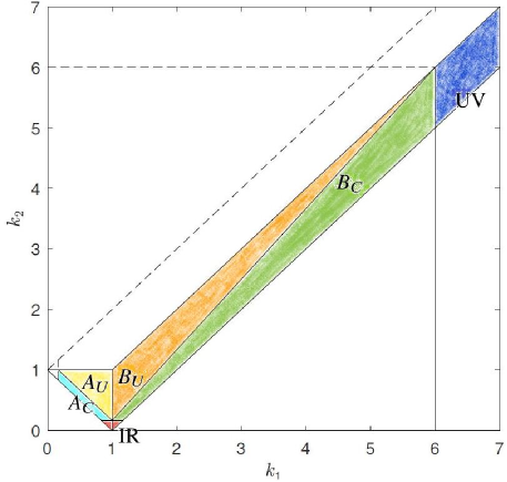
Figure 1: The kinematic box is splitted into subregions: $A_{C}$ (light blue), $A_{U}$ (yellow), $B_{C}$ (green), $B_{U}$ (orange), $\rm IR$ (red), $\rm UV$ (blue). $A_{C}$ and $B_{C}$ are the near-colinear regions, $\rm IR$ and $\rm UV$ are the extreme scale-separated regions, and $A_{U}$ and $B_{U}$ are the unclassified regions. A suitable Zakharov-Kraichnan transformation, see Eq. (18), maps the regions $B_{C}$ and $B_{U}$ into $A_{C}$ and $A_{U}$, respectively.

Exploiting symmetries, the r.h.s. of Eq. (6), which we denote by $\mathcal{I}(k,m;a,b)$ after introducing the ansatz (7), can be reorganized as follows:

$$\mathcal{I}(k,m;a,b)=\Bigg{[}\int_{A_{C}}+\int_{A_{U}}+2\left(\int_{B_{C}}+\int_{B_{U}}+\int_{\rm IR}+\int_{\rm UV}\right)\Bigg{]}\;{\cal J}(k,k_{1},k_{2},m)\;dk_{1}dk_{2}\,,$$ (14)

where a sum over the six solutions to the above resonance conditions is implicit. With $b=0$, the conditions on the exponent $a$ for convergence of the collision integral on the r.h.s. of Eq. (9) come from the infrared ($\rm IR$, red in Fig. 1) and the ultraviolet ($\rm UV$, dark blue in Fig. 1) regions of integration. The details for the computation of the following results are given in Supplementary materials [Dematteis & Lvov (2020)]. Both singularities involve a first and a second cancellations between equal and oppositely signed leading tems. For the infrared contribution, we obtain

$$\mathcal{I}_{\rm IR} \simeq-16\pi ak^{-2a+4}m\int_{0}^{k_{\rm IR}/k}dx\int_{-x}^{x}dy\;x^{-a-1}\frac{y^{2}(y^{2}-x^{2})}{\sqrt{x^{2}-y^{2}}}\ =2\pi^{2}\frac{a}{4-a}mk^{-a}k_{\rm IR}^{-a+4}\,,$$ (15)

where $k_{\rm IR}$ is the (small) height of the red region in Fig. 1. The integral converges if $a<4$. Also notice that the integral is positive. For the ultraviolet contribution, we obtain

$$\mathcal{I}_{\rm UV} \simeq-32\pi ak^{-2a+4}m\int_{0}^{k/k_{\rm UV}}dx\int_{0}^{x}dy\;\frac{k^{2}}{x^{3}}\;x^{a-8}\left[(x-y)^{4}+x^{2}(x-y)^{2}\right]/\sqrt{(2x-y)y}$$ (16)

$$\simeq-14\pi^{2}\frac{a}{a-3}k^{-a+1}m\;k_{\rm UV}^{3-a}\,,$$

where $k_{\rm UV}$ is the $k_{1}$ coordinate of the left boundary of the ultraviolet region. The integral converges when $a>3$. Note that this contribution is negative, providing possibility for this contribution to balance the positive contribution from (15). This observation will later be exploited in Section 4.2 to find the steady state solution composed of a balance of infrared and ultraviolet contributions. The contribution (15) is given by the resonance conditions $({\rm Ia})$ and $({\rm IIa})$, the infrared ID resonances, while the contribution (15) is given by the resonance conditions $({\rm IIb})$ and $({\rm IIIc})$, the ultraviolet ID resonances. Both ES and PSI resonances turn out to be subleading.

3.2 Numerical solution: $a=3.69$

Straightforward numerical integration can be performed only in $A_{\rm U}$ and $B_{\rm U}$, since close to the boundaries the integrand contains integrable singularities. For this reason, numerical integration is performed adopting the following technique for integrable singularities [Heath (2002)]. We take the leading order singularity of the integrand, integrate it analytically and add the numerical integral of the difference between the integrand and the leading order singularity. This way, the integrable singularities is integrated analytically rather than numerically, ensuring accurate results. Notice that a singular behavior is found not only in the infrared and ultraviolet regions, but also in the colinear regions, due to the vanishing denominator $\Delta_{\mathbf{p}12}$. The vanishing of denominator occurs because the area of a triangle with colinear sides tend to zero. The detail of the procedure for each of the five regions is found in Supplementary materials  [Dematteis & Lvov (2020)].

To convince the reader that the numerical integration is performed accurately, we show that the discretized integral is independent of the step size of the discretization grid for sufficiently fine grid. This is demonstrated in Supplementary materials  [Dematteis & Lvov (2020)].

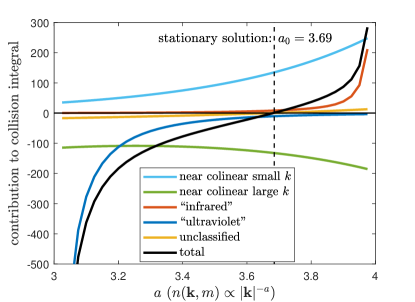
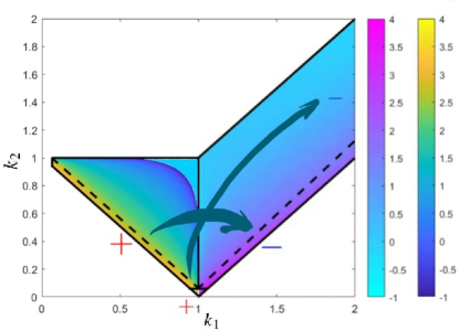
Figure 2: Left: Contributions of each subregion (as split in Eq. (14)) to the integral for $b=0$ and varying $a$. Right: The base-$10$ logarithm of the magnitude of the integrand is shown, for the solution $a=3.69$, $b=0$. The colormap labeled by the left colorbar indicates negative values, and the right colorbar indicates positive values. Also, we show here the schematic representation of the downscale energy transfers. The thicker arrow represents the stationary transfer between near-colinear regions, and the thinner arrow between regions with extreme scale separation. The fluxes of energy are explained in Section 5.

The width of the regions around $k_{2}=0$ is determined by the parameter $k_{\rm IR}$, while the cut at large $k$’s is performed at $k_{1}=k_{\rm UV}$. For the result to be general, it must be independent of the choice of $k_{\rm IR}$ and $k_{\rm UV}$, as long as they are finite numbers, $k_{\rm IR}$ being sufficiently small and $k_{\rm UV}$ sufficiently large. Iit turns out this is indeed the case in our numerics. In Supplementary materials  [Dematteis & Lvov (2020)] we show how convergence is reached as $k_{\rm UV}$ increases, as the neglected contribution in $\rm UV$ vanishes. Independence of the result upon variations of $k_{\rm IR}$ is even more robust.

According to our results, the stationary spectrum of internal waves is given by

$$n(k,m)\propto k^{-a_{0}}\,,\qquad a_{0}\simeq 3.69\,.$$ (17)

The result in Fig. 2, obtained with a choice $k_{\rm UV}=1/k_{\rm IR}=16$, confirms convergence of the collision integral for $3<a<4$: divergence of the integral is found both as $a\to 3^{+}$ and $a\to 4^{-}$. In Fig. 2, we show the contributions of each region of the kinematic box. The $a=3$ divergence is negative and due to the region $\rm UV$ (ultraviolet). The contribution of $\rm UV$ is always negative and tends to zero as $a\to 4$. On the other hand, the $a=4$ divergence is positive and due to the region $\rm IR$. The contribution of $\rm IR$ is always positive and tends to zero as $a\to 3$. At the stationary solution $a=a_{0}$ the contributions of $\rm IR$, $A_{U}$, $B_{U}$, $\rm UV$ are close to zero, while the contributions of $A_{C}$ (positive) and $B_{C}$ (negative) are large and cancel out. Notice that the results are obtained for $A_{C}$ and $B_{C}$ being thin slices of width $1/16$: the points in the colinear region correspond to triads of wave vectors that have angles between each other’s horizontal components of $3^{\circ}$ or less!

Let us consider an arbitrary reference number $k=1$. The sign of the integrand in the right panel of Fig. 2 indicates the direction of the energy transfers. We see from Fig. 2 that the contribution from the wave numbers with $k_{1}<1$ is positive. Therefore there is a net energy flow from wave numbers smaller than reference number $k=1$ to the reference wave number $k=1$. On the other hand, the contribution from the wave numbers with $k_{1}>1$ is negative. Consequently the wave number $k=1$ constantly pumps energy towards higher wave numbers. Therefore we conclude that the energy transfer is directed towards high horizontal wave numbers. We elaborate on this further in Section 5.

The outflowing energy from the small-wave-number near-colinear triads is balanced by the inflowing energy at the large-wave-number near-colinear triads, implying a stationary flow mediated by $k=1$ which is represented as a thick arrow in Fig. 2. The outflowing energy from the infrared region is balanced by the inflowing energy entering the ultraviolet region,giving a stationary energy flow between these two regions mediated by $k=1$. This energy transfer is represented as a thin directed arrow connecting the two regions. The quantitative justification of the balance is given by the left panel of Fig. 2.

The value of the exponent appears to be characterized importantly by a balance of the regions $A_{C}$ and $B_{C}$. This suggests that a suitable transformation mapping one region into the other could potentially make the search for the steady self-similar spectrum amenable to analytical treatment. This task is addressed in the next section.

4 Analysis of the contributions to the stationary solution

We consider the reorganized expression of the collision integral in Eq. (9). Let us introduce the following Zakharov-Kraichnan transformations,

$$\left\{\begin{aligned} &k_{1}=\frac{k^{2}}{\tilde{k}_{1}}\ &k_{2}=\frac{k\tilde{k}_{2}}{\tilde{k}_{1}}\end{aligned}\right.\,,\qquad\qquad\qquad\qquad\left\{\begin{aligned} &k_{2}=\frac{k^{2}}{\tilde{k}_{2}}\ &k_{1}=\frac{k\tilde{k}_{1}}{\tilde{k}_{2}}\end{aligned}\right.\,,$$ (18)

and notice that under the first transformation the regions $B_{C}$ and $B_{U}$ are mapped into $A_{C}$ and $A_{U}$, respectively, if the choice $k_{\rm UV}=k^{2}/k_{\rm IR}$ is made. In the following we consider the contributions from the three types of regions (near-colinear, extreme-scale-separated and unclassified) separately, with the goal of locating the regions and the resonances that matter the most and the ones that are negligible.

4.1 Colinear limit

We start by analyzing the contributions in the regions $A_{C}$ and $B_{C}$ by decomposing them into separate sub-contributions from the three resonance types $({\rm I})$, $({\rm II})$ and $({\rm III})$ (see Table 1). The different contributions are plotted in Fig. 3. We realize that in the region $A_{C}$ the leading contribution is given by the resonance condition $({\rm I})$, while in region $B_{C}$ the leading contribution is given by the resonance condition $({\rm II})$. Let us consider only these two contributions, naming them the main colinear contributions:

$$\mathcal{I}_{A_{C}}+2\mathcal{I}_{B_{C}}\simeq \int_{k_{\rm IR}}^{1-k_{\rm IR}}dk_{2}\int_{0}^{k_{\rm IR}}dx\frac{T^{k}_{k_{1},k-k_{1}}}{\sqrt{2kk_{1}(k-k_{1})x}}$$ (19)

$$-\int_{1+k_{\rm IR}}^{k_{\rm UV}}dk_{2}\int_{0}^{k_{\rm IR}}dx\frac{T^{k_{1}}_{k,k_{1}-k}}{\sqrt{2kk_{1}(k_{1}-k)x}}-\int_{1+k_{\rm IR}}^{k_{\rm UV}}dk_{2}\int_{0}^{k_{\rm IR}}dx\frac{T^{k_{2}}_{k,k_{2}-k}}{\sqrt{2kk_{2}(k_{2}-k)x}}\,,$$

where $T^{0}_{12}=kk_{1}k_{2}|V^{0}_{12}|^{2}f^{0}_{12}/|{g^{0}_{12}}^{\prime}|\,.$ Transforming the integral into an integral in the region $A_{C}$, by using the symmetries of Eq. (18) (with $k_{\rm UV}=k^{2}/k_{\rm IR}$) and the scale-invariant properties of the integrand, we obtain (renaming $\tilde{k}_{1}\rightarrow k_{1}$, $\tilde{k}_{2}\rightarrow k_{2}$)

$$\mathcal{I}_{A_{C}}+2\mathcal{I}_{B_{C}}\simeq\int_{0}^{k_{\rm IR}}dx\int_{k_{\rm IR}}^{1-k_{\rm IR}}dk_{2}\frac{T^{k}_{k_{1},k-k_{1}}}{\sqrt{2kk_{1}(k-k_{1})x}}\left[1-\left(\frac{k}{k_{1}}\right)^{r+3}-\left(\frac{k}{k_{2}}\right)^{r+3}\right]\,,$$ (20)

where $r$ is the degree of homogeneity of the integrand: $r=3-2a$ (same dependence on $k$ as in the computation of the Pelinovski-Raevski spectrum). We used the property of the Zakharov-Kraichnan transformation for an homogeneous function of degree $r$ with respect to horizontal wave numbers:

$$\mathcal{J}\left(k_{1},k,k_{2},m\right)=\mathcal{J}\left(\frac{k}{\tilde{k}_{1}}k,\frac{k}{\tilde{k}_{1}}\tilde{k}_{1},\frac{k}{\tilde{k}_{1}}\tilde{k}_{2},m\right)=\left(\frac{k}{\tilde{k}_{1}}\right)^{r}\mathcal{J}\left(\tilde{k},\tilde{k}_{1},\tilde{k}_{2},m\right)\,,$$ (21)

and a factor $(k/\tilde{k_{1}})^{3}$ appeared due to the Jacobian of the coordinate change. Now, we notice that if $r+3=-1$, the integrand contains a factor $[k-k_{1}-k_{2}]$. Since we are considering the near-colinear region, horizontal momentum conservation implies that such a factor vanishes (more precisely, it would vanish in the limit $k_{\rm IR}\to 0$): $A_{C}$ is a thin slice lying on the line $k_{2}=k-k_{1}$. Therefore, we have that $\mathcal{I}_{A_{C}}+2\mathcal{I}_{B_{C}}=0$ for $6-2a=-1$, which determines the value of $a=7/2$ as the critical exponent .

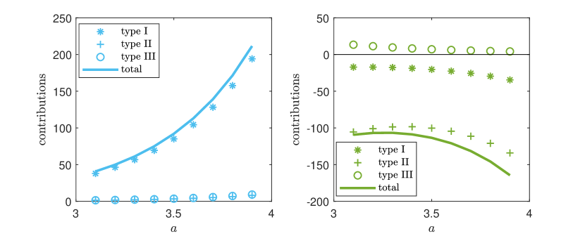
Figure 3: The contributions from $A_{C}$, left panel, and $B_{C}$, right panel (the latter multiplied by $2$ to account for its symmetric $B_{C}^{\prime}$ by permutation $k_{1}\leftrightarrow k_{2}$), are splitted into their sub-contributions from the three resonance types, showing that $A_{C}$ is dominated by the contribution $({\rm I})$, while $B_{C}$ is dominated by the contribution $({\rm II})$. Computing the balance between these two contributions leads to a theoretical estimate $a=7/2$.

We have therefore found analytically the steady state solution for the reduced kinetic equation dominated by the balance between the contribution of type $({\rm I})$ in the region $A_{C}$ and the contribution of type $({\rm II})$ in the region $B_{C}$, which are the largest contributions from the near-colinear regions. This solution is therefore given by

$$n(k,m)=k^{-\frac{7}{2}}m^{0}\,.$$ (22)

Since this solution is close to the Pelinovsky-Raevsky spectrum (8), we propose to call this solution modified Pelinovsky-Raevsky spectrum. The difference between (22) and (8) is that the latter is the formal solution, corresponding to a non-local spectrum (i.e., implying a divergent collision integral). The former solution, on the other hand, is a physically relevant solution corresponding to a local action spectrum (i.e., whose collision integral is finite). Note, however that a part of the resonances have been neglected.

The result $a=7/2$ coming from the colinear limit of Eq. (20) involves only the two leading contributions in Fig. 3. This observation provides an intuition on how the exponent $a$ is determined by the kinetic equation. The sum of the subdominant contributions in Fig. 3 is negative and almost independent of $a$. When added to the main contribution crossing zero at $a=7/2$, this negative contribution makes the zero-crossing point shift toward the right and in Fig. 4(A) the total colinear contribution is shown to cross zero at $a\simeq 3.69$.

4.2 Extreme-scale-separated triads

In this section we consider the contribution that comes from the extreme-scale-separated triads, the sum of the infrared and the ultraviolet contributions. The former is positive and tends to $+\infty$ as $a\to 4^{-}$; the latter is negative and tends to $-\infty$ as $a\to 3^{+}$. In Fig. 4(A) we show the total contribution of the extreme-scale-separated resonances and we observe numerically that it crosses zero around $a\simeq 3.69$, too.

A	B

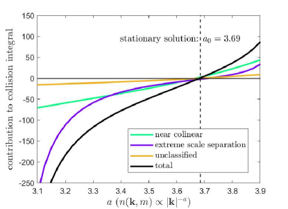
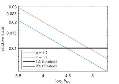
Figure 4: A The net contribution of the three types of triads, showing that each type balances to zero independently at the convergent stationary solution. B Relative error of Eq. (16) with respect to the fully numerically integrated contribution of region ${\rm UV}$. Around $a=3.7$, we see that a choice of $k_{\rm UV}=16$ ($y=4$) implies an error of about $2\%$, which we consider acceptable. Thus, we consider $k_{\rm UV}=16$ as a reasonable delimitation of the ultraviolet region, as well as $k_{\rm IR}=1/16$ as the delimitation of the infrared region.

In Section 3.1 we proposed a balance between positive infrared (15) and negative ultraviolet (16) contributions as a way to form the steady state spectrum of internal waves. This balance hinges upon the choice $k_{\rm UV}=k^{2}/k_{\rm IR}$, as explained in Section 4.1.

In Fig. 4, we show the relative error of the leading order analytical expression (16), with respect to the numerically computed contribution, as a function of $k_{\rm UV}$. The result is shown for $a=3.5$ and $a=3.7$. Using the expression $k_{\rm UV}=2^{y}$, with $k=1$, we observe that the analytical approximation is good starting from values of $y$ between $4$ and $5$. We choose $y$ (and therefore $k_{\rm UV}$ and $k_{\rm IR}$) large enough for an accurate approximation with the leading order expression (16) (or (15)), yet small enough so that all extreme-scale-separated triads ((16)) and ((15)) are actually included in the ultraviolet and infrared regions. We make an arbitrary choice $y=4$ ($k_{\rm UV}=1/k_{\rm IR}=16$) so that the leading order error of ((15)) and ((16)) is about 2 percent (see Fig. 4). Our results are insensitive to this specific choice. The balance between the two expressions gives

$$2\pi^{2}\frac{a}{4-a}k_{\rm IR}^{4-a} =14\pi^{2}\frac{a}{a-3}\frac{1}{k_{\rm IR}^{3-a}}$$ (23)

$$h_{y}(a):=(2a-7)y\log 2 =\log 7+\log\left(\frac{4-a}{a-3}\right)=:g(a)\,.$$

First, we notice that the presence of a factor $7$ on the r.h.s. breaks the symmetry that would imply the two contributions to balance out at $a=7/2$, in the middle of the convergence interval $(3,4)$. Secondly, we notice that the function $g(a)$ has an inflection point at $a=7/2$, making its Taylor expansion of first order have an error of third order. Using linear interpolation centered at $a=7/2$, $g_{7/2}(a)=\log 7-2(2a-7)$, as an accurate approximation to $g(a)$, demanding that $h_{y}(a)=g_{7/2}(a)$ we obtain

$$a=\frac{7}{2}+\frac{\log 7}{2y\log 2+4}\,.$$ (24)

If we adopt $y=4$, as chosen throughout the paper, we obtain the solution $a\simeq 3.70$. Using $y=5$ would yield a solution $a\simeq 3.68$.

In this section, we have shown how the formation of the stationary solution of the wave kinetic equation can be interpreted via two independent balances, between near-colinear triads and between the ID triads of the extreme-scale-separated regions. This is consistent with recent results from direct numerical simulations where the dominating interactions were located in the ID regime but also throughout all of the interval $k_{1}\in[0,1.4k]$ [Pan et al. (2020)]. Despite the latter effect was there investigated as a broadening of ID due to large nonlinearity, we find that it may be consistent with the colinear resonances depicted in the right panel of Fig. 2.

5 Downscale energy transfers

5.1 Physical dimensions and energy conservation

Using the scale-invariant properties of the collision integral, the r.h.s. of Eq. (9) can be rewritten considering the appropriate physical dimensions as

$$I(\mathbf{k},m)=|m|^{-2b+1}k^{-2a+4}(V_{0}A)^{2}\mathcal{I}(k=1,m=1;a,b)\,,$$ (25)

where $\mathcal{I}(k=1,m=1;a,b)$ is non-dimensional, $V_{0}$ is the dimensional prefactor of the matrix element defined below in Eq. (29), and $A$ is the prefactor of the Garrett and Munk spectrum defined in (2) above. A simple way to check the dimensional consistency of the prefactor in (25) is to consider the contribution from the extreme-scale-separated region, Eq. (23), which is analytically tractable:

$$2\pi^{2}\frac{a}{4-a}k^{-a}k_{\rm IR}^{4-a}-14\pi^{2}\frac{a}{a-3}\frac{k^{-a+1}}{k_{\rm IR}^{3-a}}=mk^{-2a+4}\left(2\pi^{2}\frac{a}{4-a}x_{\rm IR}^{4-a}-14\pi^{2}\frac{a}{a-3}x_{\rm IR}^{a-3}\right)\,,$$ (26)

where $x_{\rm IR}=k_{\rm IR}/k$ and the term in brackets is a nondimensional function of the exponent $a$ that vanishes at $a=a_{0}$. The factor $(V_{0}A)^{2}$ comes from having both the matrix elements and the spectrum to the second power in the collision integral, and by introducing the appropriate dimensional constants that have been omitted so far. The dimensional properties of the collision integral are indeed the same also in the other integration regions.

Next, we compute the spectral energy fluxes, recalling that the energy density is given by

$$e(k,m)=2\pi k\sigma(\mathbf{k},m)n(\mathbf{k},m)\,,\qquad\sigma(\mathbf{k},m)=\alpha\frac{k}{|m|}\,,\;\text{ with }\;\;\alpha=\frac{g}{\rho_{0}N}\,,$$ (27)

where the scale invariant dispersion relation (4) is used. Using (25), the stationary wave kinetic equation for the energy density assumes the simple form

$$\dot{e}(k,m)=2\pi(AV_{0})^{2}k^{-2a+6}m^{-2b}\mathcal{I}(k=1,m=1;a,b)=0\,.$$ (28)

5.2 Dimensional prefactors

The dimensional factor coming from the matrix elements in Eq. (25) is given by

$$|V_{0}|^{2}=\frac{N}{\color[rgb]{0,0,0}32\rho_{0}}\,.$$ (29)

The factor $A$ is the dimensional prefactor of the GM spectrum, our observational input for the oceanic wave field. The procedure to obtain $A$ is explained in the rest of this paragraph. The non-rotating limit of the GM spectrum in $k-m$ coordinates is given by Eq. (3). However, in isopycnal coordinates the spectrum needs to be multiplied by a factor $N^{2}\rho_{0}/g$, which gives

$$n_{\rm GM}(k,m)=\frac{{\color[rgb]{0,0,0}1}}{\pi^{3}g}Eb^{2}{\color[rgb]{0,0,0}N_{0}N}\rho_{0}fm_{\star}k^{-4}\,,\qquad m_{\star}=3\pi\frac{N}{bN_{0}}\,,$$ (30)

where $E=6.3\times 10^{-5}$ is the non-dimensional energy level, $b=1300$ m, $\rho_{0}=1000$ kg$/$m³, $N_{0}=0.00524$ s^-1, $f=2\cdot 7.3\times 10^{-5}\sin(l)$ (at latitude $l=32.5^{\circ}$). The values given here are the ones of the standard GM parametrization. Since for the GM spectrum we have $a=4$ instead of $a=3.69$, we introduce the modified version of Eq. (30):

$$n_{\rm GM,c}(k,m)=\frac{{\color[rgb]{0,0,0}1}}{\pi^{3}g}Eb^{2}{\color[rgb]{0,0,0}N_{0}N}\rho_{0}f\frac{m_{\star}}{{k_{\star}}^{(1-s)/2}}k^{-(4-(1-s)/2)}\,,\quad k_{\star}=m_{\star}/r\,,$$ (31)

where $s=2a-7=0.38$. This is a slightly less steep, dimensionally consistent version. The non-dimensional parameter $r={\color[rgb]{0,0,0}N}/f$ quantifies the horizontal-to-vertical anisotropy, [Polzin & Lvov (2011)]. Now, the GM spectrum is normalized so that the total energy is expressed in units of J$/$kg, as usual in physical oceanography. On the other hand, in the wave turbulence formalism the total energy is expressed as a density per unit of volume of the physical space. Here, the physical space has units of ${\rm kg}/{\rm m}$, given by an area in the horizontal directions times a density in the vertical. It is therefore possible to switch from one representation to the other multiplying by the appropriate density, which in this case is the characteristic density of the isopycnal coordinates, ${\color[rgb]{0,0,0}\Pi=g/N}^{2}$, in units of meters (normalized differential thickness of an isopycnal layer). This results into the equivalence: $n_{\rm WKE}=n_{\rm GM}\cdot g/{\color[rgb]{0,0,0}N}^{2}$, which applied to (31) finally gives the dimensionally consistent factor

$$A=\frac{{\color[rgb]{0,0,0}1}}{\pi^{3}}Eb^{2}\rho_{0}f{\color[rgb]{0,0,0}\frac{N_{0}}{N}}\frac{m_{\star}}{k_{\star}^{(1-s)/2}}\,.$$ (32)

5.3 Dissipated power at high wave numbers

In order to compute the energy flux towards high wave numbers we need to consider the physical cutoffs of the problem. Natural cutoffs are imposed on the vertical wave number by the depth of the ocean and by the wave breaking cut off, and on the frequency by the inertial frequency and the buoyancy frequency,

$$m_{\rm min}=\frac{2\pi g}{\rho_{0}N^{2}}\times(2600\text{ m})^{-1}\,\quad m_{\rm max}=\frac{2\pi g}{\rho_{0}N^{2}}\times(10\text{ m})^{-1}\,,\quad\sigma_{\rm min}=f\,,\quad\sigma_{\rm max}=N\,.$$ (33)

These limiting values define a rectangle in $\sigma-m$ space that translates into a trapezoid in $k-m$ space, with inclined sides given by

$$k_{\rm min}(m)=\frac{f}{\alpha}m\,,\quad k_{\rm max}(m)=\frac{N}{\alpha}m\,.$$ (34)

The collision integral contains all of the necessary information on the spectral energy transfers. In the following, we compute numerically the outflowing power at high wave numbers from computation of the contribution of the resonant triads with an output wave number such that $m>m_{\max}$ or $k>k_{\max}(m)$, i.e. assuming that the production of a wave beyond the physical high wavenumber cutoff results into complete dissipation of its energy. At the same time, it is assumed that the region within the physical cut-offs is an inertial range with no sources nor sinks, where energy is transfered exclusively via resonant interactions.

Let us define the part of the collision integral which contributes to the dissipation of energy by transferring it beyond the dissipation cut-offs:

$$I_{\rm diss}(\mathbf{k},m;k_{\max}): =\frac{{{\color[rgb]{0,0,0}N}}^{2}}{g}(V_{0}A)^{2}\alpha^{-1}|m|^{-2b+1}k^{-2a+4}\mathcal{I}_{\rm diss}(\kappa)\,,$$ (35)

$$\mathcal{I}_{\rm diss}(\kappa) =\int_{\Omega_{\rm h}(\kappa)}\mathcal{J}(k=1,k_{1},k_{2},m=1)dk_{1}dk_{2}\,,$$

where $\kappa=k_{\max}/k$ and $\Omega_{\rm h}(\kappa)$ as the set of triads transferring energy to output waves beyond the horizontal dissipation cutoff $k_{\max}$, and is defined in Table 2. Moreover, a factor $\frac{{{\color[rgb]{0,0,0}N}}^{2}}{g}$ is added to account for transition to isopycnal coordinates, the inverse of the factor in Eq. (32). Here, $I_{\rm diss}(\mathbf{k},m;k_{\max})$ quantifies the amount of wave action that wave number $\mathbf{p}$ sends via resonant interactions beyond the dissipation threshold $k_{\max}$, per unit time and per unit volume of Fourier space.

Input	Output	$\Omega_{\rm h}(\kappa)$	$\Omega_{\rm v}(\mu)$
$\mathbf{p}$	$\mathbf{p}_{1},\mathbf{p}_{2}$	$\left.\begin{array}[]{l}k_{1}>\kappa,k_{2}>\kappa\\ k_{1}>\kappa,k_{2}<\kappa:\text{ weight }\tfrac{\sigma_{1}}{\sigma_{1}+\sigma_{2}}\\ k_{1}<\kappa,k_{2}>\kappa:\text{ weight }\tfrac{\sigma_{2}}{\sigma_{1}+\sigma_{2}}\end{array}\right.$	$\left.\begin{array}[]{l}|m_{1}|>\mu,|m_{2}|>\mu\\ |m_{1}|>\mu,|m_{2}|<\mu:\text{ weight }\tfrac{\sigma_{1}}{\sigma_{1}+\sigma_{2}}\\ |m_{1}|<\mu,|m_{2}|>\mu:\text{ weight }\tfrac{\sigma_{2}}{\sigma_{1}+\sigma_{2}}\end{array}\right.$
$\mathbf{p},\mathbf{p}_{2}$	$\mathbf{p}_{1}$	$k_{1}>\kappa,k_{2}<\kappa$	$|m_{1}|>\mu,|m_{2}|<\mu$
$\mathbf{p},\mathbf{p}_{1}$	$\mathbf{p}_{2}$	$k_{1}<\kappa,k_{2}>\kappa$	$|m_{1}|<\mu,|m_{2}|>\mu$

Table 2: All of the non-negligible contributions for $\kappa>1$ are negative (see right panels of Figs. 2-3). The same holds for $\mu>1$. Thus, wave number $\mathbf{p}$ is always an incoming wave in the triads here considered. The table represents the conditions under which every type of resonance results into the dissipation of energy due to at least one output beyond the dissipation cutoffs. During the numerical computation of the integrals $C_{\rm h}$ and $C_{\rm v}$, these conditions are applied for every point of the kinematic box. In the case of a decay into two waves of which only one is dissipated, only the fraction of energy of the dissipated wave must be accounted for, multiplying the contribution by the weight shown in the table.

The power (per unit of $m$) dissipated beyond $k_{\max}$ at fixed $m$ (now considered as the positive definite magnitude of $m$) is related to the integral of $I_{\rm diss}(\mathbf{k},m)$ for all values of $k$:

$$F_{\rm diss}(m) =\int_{k_{\min}}^{k_{\max}}{\color[rgb]{0,0,0}4}\pi k\omega(\mathbf{p})I_{\rm diss}(\mathbf{k},m;k_{\max})dk\,$$ (36)

$$=\frac{{{\color[rgb]{0,0,0}N}}^{2}}{g}\int_{k_{\min}}^{k_{\max}}{\color[rgb]{0,0,0}4}\pi|m|^{-2b+1}k^{-2a+5}\alpha\frac{k}{|m|}(V_{0}A)^{2}\alpha^{-1}\mathcal{I}_{\rm diss}(\kappa)$$

$$={\color[rgb]{0,0,0}4}\pi\frac{{{\color[rgb]{0,0,0}N}}^{2}}{g}(V_{0}A)^{2}k_{\max}^{-s}C_{\rm h}\,,\quad\text{with}\qquad C_{\rm h}:=\int_{1}^{\frac{N}{f}}\kappa^{s-1}\mathcal{I_{\rm diss}(\kappa)}\,,$$

where we recall that $s=2a-7=0.38$, and $b=0$. In a similar fashion, we can obtain an analogous relation for the energy flux dissipated vertically at vertical wave numbers larger than $m_{\max}$:

$$G_{\rm diss}(k)={\color[rgb]{0,0,0}4}\pi\frac{{{\color[rgb]{0,0,0}N}}^{2}}{g}(V_{0}A)^{2}k^{-(1+s)}{m_{\max}}C_{\rm v}\,,\qquad C_{\rm v}:=\int_{1}^{\frac{m_{\max}}{m_{\min}}}\mu^{-2}\mathcal{K_{\rm diss}(\mu)}\,,$$ (37)

$$\qquad\qquad\mathcal{K}_{\rm diss}(\mu)=\int_{\Omega_{\rm v}(\kappa)}\mathcal{J}(k=1,k_{1},k_{2},m=1)dk_{1}dk_{2}\,,$$

where $\mathcal{K}_{\rm diss}(\mu)$ is the analogue of $\mathcal{I}_{\rm diss}(\kappa)$ in the vertical direction, i.e. the collision integral restricted to the triads with output waves beyond the $m_{\max}$ threshold. The conditions defining $\Omega_{\rm v}$ are found in Table 2. These integrals are computed numerically. The computation of $C_{\rm h}$ is quite straightforward since the kinematic box is expressed in horizontal wave number coordinates. The quantity $\mathcal{I}_{\rm diss}(\kappa)$ is computed inside a loop spanning all values of $\kappa$, checking the constraint of $\Omega_{\rm h}(\kappa)$ for every point. Note that since the position of the right boundary depends on $m$, (34), in the computation of $\mathcal{I}_{\rm diss}(\kappa)$ we have to impose that $k_{1}>k_{\max}m_{1}/m$ (or the same for $k_{2}$) for point $(k_{1},m_{1})$ to be past the absorbing boundary. For the computation of $C_{\rm v}$, on the other hand, at every loop iteration we have to integrate over all of the kinematic box to compute $\mathcal{K}_{\rm diss}$ and check point by point whether $m_{1}$ or $m_{2}$ have “crossed” the boundary at $m_{\max}$ (which is independent of $k$).

One important point requires particular care. In the previous sections we relied upon the leading order of the infrared contribution of Eq. (15), which is obtained after the second cancellation where a negative singularity for $k_{1}>1$ cancels exactly with a positive singularity for $k_{1}<1$. However, since now in Eq. (35) we consider an integration region where $k_{1}>\kappa>1$, the positive singularity due to $k_{1}<1$ is no longer present and thus the use of Eq. (15) is not justified. In the integrand of Eq. (35), whose expression is found in the Supplementary materials [Dematteis & Lvov (2020)], the finite point singularity therefore has exponent $-a+3/2$ rather than the $-a+2$ resulting after the second cancellation (leading to Eq. (15)). Integrating twice according to Eq. (35), the exponent of the singularity of the integrand defining $C_{\rm h}$ in Eq. (36) is $\beta_{\rm h}=-a+7/2\simeq 0.19$ . Numerical computation of $\mathcal{I}_{\rm diss}(\kappa)$ as $\kappa\to 1^{+}$ confirms this analytical prediction and gives a best least square fit of $\mathcal{I}_{\rm diss}(\kappa)\sim-d_{\rm h}(\kappa-1)^{-\beta_{\rm h}}$, for $\kappa-1\ll 1$, with $d_{\rm h}={\color[rgb]{0,0,0}127}\times 8\pi$, $\beta_{\rm h}=0.19$. An analogous computation for the integral $C_{\rm v}$ defined in Eq. (37) leads to a best fit scaling of its integrand of $\mathcal{K}_{\rm diss}(\mu)\sim-d_{\rm v}(\mu-1)^{-\beta_{\rm v}}$, for $\mu-1\ll 1$, with $d_{\rm v}\simeq 9.0\times 8\pi$, $\beta_{\rm v}\simeq 0.75$. In this case, an analytical evidence of the exponent is not simply available since the kinematic box is not expressed in vertical wave number coordinates. In Fig. 5, we show the rapidly decaying behaviour of the integrands of $C_{\rm h}$ and $C_{\rm v}$. Therefore, $C_{\rm h}$ and $C_{\rm v}$ are “universal constants” which are relatively insensitive to the limits of integration in Eqs. (36)-(37). The figure also shows a closer look to the scaling of the singularities as $\kappa\to 1^{+}$ and $\mu\to 1^{+}$, with the respective best fit scalings. Therefore we obtain:

$$C_{\rm h}\simeq\int_{1}^{\frac{N}{f}}\kappa^{s-1}\mathcal{I_{\rm diss}(\kappa)} \simeq-\frac{d_{\rm h}\,{k_{\rm IR}}^{1-\beta_{\rm h}}}{1-\beta_{\rm h}}+\int_{1+k_{\rm IR}}^{\frac{N}{f}}d\kappa\,\kappa^{s-1}\mathcal{I}_{\rm diss}(\kappa)$$ (38)

$$\simeq-8\pi{\color[rgb]{0,0,0}(16.6+54.6+10.2)\simeq-8\pi\times 81.4}\,.$$

Here the three numbers $16.6$, $54.6$ and $10.2$ represent the partial contributions by the infrared ID interactions, near-colinear interactions and unclassified interactions, respectively. The ultraviolet contribution is negligible.

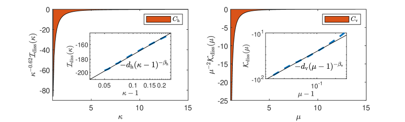
Figure 5: The two panels show the integrands of $C_{\rm h}$ and $C_{\rm v}$, respectively, and the areas colored in red represent $C_{\rm h}$ and $C_{\rm v}$ themselves. Both integrals have a finite point integrable singularity (the exponents $\beta_{\rm h}$ and $\beta_{v}$ are in the interval $(0,1)$) at their left boundaries: the insets show the asymptotic power-law scaling of the singularities.

Then, choosing a value $\mu_{\rm IR}=1/16$ to delimit the infrared region for vertical wave numbers, we have

$$C_{\rm v}\simeq\int_{1}^{\frac{m_{\max}}{m_{\min}}}\mu^{-2}\mathcal{K_{\rm diss}(\mu)} \simeq-\frac{d_{\rm v}\,{\mu_{\rm IR}}^{1-\beta_{\rm v}}}{1-\beta_{\rm v}}+\int_{1+\mu_{\rm IR}}^{\frac{m_{\max}}{m_{\min}}}d\mu\,\mu^{-2}\mathcal{K}_{\rm diss}(\mu)$$ (39)

$$\simeq-8\pi(18.0+14.0+3.1)\simeq-8\pi\times 35.1\,.$$

Again, the numbers $18.0$, $14.0$ and $3.1$ represents infrared (ID), near-colinear and unclassified contributions, respectively, with a negligible contribution from the ultraviolet regions.

Now, we compute the power crossing the $k_{\max}$ boundary, denoted as $P_{\rm h}$ (horizontal boundary), and the power crossing the $m_{\max}$ boundary, denoted as $P_{\rm v}$ (vertical boundary), via

$$P_{\rm h}=\int_{m_{\rm min}}^{m_{\rm max}}F_{\rm diss}(m)\;dm=D_{\rm h}(1-s)^{-1}\left(\frac{N}{\alpha}\right)^{-s}(m_{\rm max}^{1-s}-m_{\rm min}^{1-s})\,,$$ (40)

$$P_{\rm v}=\int_{\frac{f}{\alpha}m_{\max}}^{\frac{N}{\alpha}m_{\max}}G_{\rm diss}(k)\;dk=D_{\rm v}s^{-1}\left[\left(\frac{f}{\alpha}\right)^{-s}-\left(\frac{N}{\alpha}\right)^{-s}\right]m_{\rm max}^{1-s}\,,$$

where

$$D_{\rm h}={\color[rgb]{0,0,0}4}\pi\frac{{{\color[rgb]{0,0,0}N}}^{2}}{g}(V_{0}A)^{2}C_{\rm h}\,\quad D_{\rm v}={\color[rgb]{0,0,0}4}\pi\frac{{{\color[rgb]{0,0,0}N}}^{2}}{g}(V_{0}A)^{2}C_{\rm v}\,,$$ (41)

Using (29), (32), (40) and (41), we obtain

$$P_{\rm h}=\frac{\Gamma C_{\rm h}}{1-s}\;{\color[rgb]{0,0,0}\left[1-\left(\frac{\ell}{2b}\right)^{s}\right]}\;{\color[rgb]{0,0,0}f^{1+s}}N^{2}E^{2}\,,$$ (42)

$$P_{\rm v}=\frac{\Gamma C_{\rm v}}{s}\;\left[1-\left(\frac{f}{N}\right)^{s}\right]\;f{\color[rgb]{0,0,0}N^{1+s}}E^{2}\,,$$

$$\Gamma={\color[rgb]{0,0,0}{\frac{3}{4\pi^{3}}}\left(\frac{{3}\ell}{2b}\right)^{s}\frac{\rho_{0}b^{2}{N_{0}^{1-s}}}{g\ell}\,,\qquad s=0.38\,,\quad\ell=10{\rm\,m}}.$$

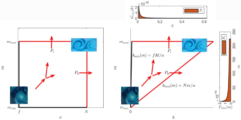
Figure 6: Left: the inertial box in $\sigma-m$ space. Right: the inertial box in $k-m$ space. The low frequency energy forcing is represented in the picture a mesoscale eddy, while wave breaking (with generation of turbulent vortices) represents dissipation at high wave numbers. The distribution of energy dissipation along the absorbing boundaries is depicted in the two insets showing $F_{\rm diss}(m)$ and $G_{\rm diss}(k)$, whose integrals (red area) give respectively $P_{\rm h}$ and $P_{\rm v}$, Eq. (40). In these two plots, $k$ is in units of ${\rm m}^{-1}$, $m$ is in units of ${\rm m}^{3}{\rm kg}^{-1}$, $G_{\rm diss}(k)$ is in $\rm{W}\,{\rm m}\,{\rm kg}^{-1}$, $F_{\rm diss}(m)$ is in $\rm{W}\,{\rm m}^{-3}$, so that both integrals give a power per unit mass.

In Fig. 6 a graphical interpretation of the computations in the above paragraph is shown. The physical cutoffs define a rectangular box (left panel) within which energy is transfered through resonant interactions toward high vertical wave numbers and high horizontal wave numbers. If energy is provided by large scale forcing at low frequency, for simplicity represented as a mesoscale eddy in the figure, it ends up being dissipated at high frequencies or high wave numbers, represented as wave breaking with generation of turbulent vortices. In $k-m$ space this inertial box translates into a trapezoid whose lateral sides are straight lines defined by the dispersion relation. The integrals in Eq. (40) quantify the contribution to the dissipated power along the dissipative sides of the box. In the figure, the red areas quantify how dissipation is distributed along these dissipative sides of the inertial box.

Eq. (42) is the main result of our paper. The outgoing power toward large wave numbers is the quantity that is modelled by the finescale parametrization formula of ocean mixing [Polzin et al. (1995)] as

$$P_{\rm fs}=(1.9\times 10^{7}\,\text{\rm m}^{2})\,\cosh^{-1}\left(\frac{N}{f}\right)\,fN^{2}E^{2}\,,$$ (43)

which is in agreement with (42) regarding the dependence upon the main physical parameters, if the lower-order corrections $(f/N)^{s}$ and $\cosh^{-1}(N/f)$ are neglected. The predicted intensities can also be compared directly, using the standard parameters of the GM spectrum (30) with $N=N_{0}$, which yields

$$P_{\rm h}\simeq-{\color[rgb]{0,0,0}0.5}\times 10^{-8}\,\text{\rm W kg}^{-1}\,,$$ (44)

$$P_{\rm v}\simeq-{\color[rgb]{0,0,0}1.5}\times 10^{-8}\,\text{\rm W kg}^{-1}\,$$

This amounts to a total dissipated power

$$P_{\rm tot}=P_{\rm h}+P_{\rm v}\simeq-{\color[rgb]{0,0,0}2.1}\times 10^{-8}\,\text{\rm W kg}^{-1}\,,$$ (45)

which is negative since it is lost by the wave system considered. With the same parameters and the same sign convention, the finescale parametrization formula predicts a total dissipated power

$$P_{\rm fs}\simeq-0.8\times 10^{-9}\,\text{\rm W kg}^{-1}\,.$$ (46)

These two predictions are in qualitative agreement, but with a difference of about an order of magnitude. We elucidate on possible reasons in the conclusions. Moreover, the following remarks are important for the sake of clarity.

Above, we have used the terminology dissipated power to indicate the amount of energy that is absorbed by the boundary sink at small scales. As far as the internal wave kinetic equation is concerned, this sink is acting as an actual dissipation term. In the finescale parametrization picture to which we refer (see [Polzin et al. (2014)], Sec. 2), this amount of energy is converted into turbulent kinetic energy at small scales, and therefore roughly equals the turbulent energy production. In turn, the latter contributes separately both to diapycnal mixing and to heat production, in proportions that can be quantified by closure assumptions beyond the scope of the present paper. We stress that the use of the word dissipation in this paper does not refer to dissipation of energy as heat, but to the role played by the sink that takes energy out of the wave system considered.

The energy fluxes at the boundaries, Eqs. (36)-(37), show a non-trivial dependence on the variables $k$ and $m$. In non-isotropic systems, rather than one single stationary state it is common to have a family of stationary states ([Nazarenko (2011)], Sec. 9.2.5) whose energy fluxes depend on $k$ and $m$ in different ways. The generalized Kolmogorov-Zakharov spectrum (that is the Pelinovski-Raevski spectrum, for internal waves) is only one among the members of the family. Then, the locality conditions imply that for the internal waves only one solution is physically meaningful, i.e. $(a,b)=(3.69,0)$. Indeed, since the solution is stationary, for any enclosed region in $k-m$ space (contained in the inertial range where no sources or sinks are present), the incoming energy flux must be equal to the outgoing energy flux (and opposite in sign). Equivalently, as long as both ends of a boundary are fixed, the total outgoing flux through the boundary must be independent of the path of the boundary in $k-m$ space. For instance, one could show that the flux through the dissipative boundary equals the flux through the forcing boundary (respectively, the red and the black boundaries in Fig. 6).

Finally, we acknowledge the fact that the solutions with $b=0$ are known in the literature as no flux solutions to the Fokker-Planck (diffusive) approximation to the kinetic equation (9). How this approximation is achieved is shown for instance in [Lvov et al. (2010)], by use of a straightforward leading order approximation of the infrared Induced Diffusion interactions. An exact leading-order balance makes the infrared flux apparently vanish, whose trace in this paper is found in the two exact cancellations in the infrared region. However, our computations leading to Eq. (15) show how the next leading order terms carry a small but non-zero flux toward high horizontal wave numbers. Moreover, a net energy flux is indeed due to interactions outside the infrared region, such as the colinear interactions. Therefore, there is no mathematical contraddiction in having $b=0$ and a nonzero downscale energy flux. Indeed, the considerations in the present paper go way beyond the diffusive approximation to the internal wave kinetic equation, where the concept of no flux solutions was concocted.

6 Discussion and conclusions

This paper is focused on the specific case of a scale invariant field of internal waves in the ocean with vertically homogeneous ($b=0$) wave action. For such a case we have found that

$\bullet$ There necessarily exists a stationary state for $3<a<4$ dictated by the opposite signs of the infrared and ultraviolet resonant singularities.

$\bullet$ The dominant contributions to the integrand of the kinetic equation are coming from Induced Diffusion and near-colinear resonances;

$\bullet$ Both near-colinear and extreme-scale-separated resonances are subject to subtractive cancellation between differing triad types;

$\bullet$ Both types of resonances balance to zero for $a\simeq 3.69$ independently, cf. Fig. 4(A);

$\bullet$ The contribution from the unclassified resonances is negligible, although it balances to zero at $a\simeq 3.69$, too;

$\bullet$ We point out an important role played by colinear resonances, and we find a modified Pelinovsky-Raevsky spectrum, Eq. (22), from a balance of the largest colinear contributions. Curiously, this solution is precisely in the middle of the interval of values of the exponent for which the collision integral is convergent, [Zakharov et al. (1992)]. With the help of this analytical result, we explained how the exponent $3.69$ appears concerning the near-colinear region. It is a result of a shift of the balance of the modified Pelinovsky-Raevsky spectrum due to the negative contribution from the subleading colinear triads.

$\bullet$ By considering the sign of the integrand of the kinetic equation we can visualize a downscale flux of energy in the horizontal wave number space, see Fig. 2.

$\bullet$ Modifying the scale invariant spectrum (17) to include natural physical boundaries in Fourier space we numerically calculate the value of the spectral flux of energy towards high horizontal and vertical wave numbers. This quantitative estimate might be useful for a direct estimate of turbulent energy mixing in the ocean.

$\bullet$ Our results compares favorably with the finescale parametrization formula of [Polzin et al. (1995)], reproducing the correct order of magnitude.

Our results are obtained for a scale invariant internal wave field with vertically homogeneous wave action profile. This profile is close to the scale invariant limit of the Garrett and Munk spectrum, yet it is a strong idealization of the actual internal wave spectrum. Generalizing the evaluations presented in this paper for more realistic ocean internal wave spectra, including the presence of background rotation and spatial inhomogeneity, is a subject of current research.

Supplementary material

7 Infrared and ultraviolet singularities

7.1 Infrared singularity

In the region ${\rm IR}$, in red in Fig. 9, let us change variables using

$$k_{1}=k(1+y),\qquad k_{2}=kx\,,$$ (47)

which gives the new integration area shown in the left panel of Fig. 7, with $x,y=O(\epsilon),\epsilon\ll 1$. Now, using a power-series expansion the factor $f^{0}_{12}$, we notice that the dominant matrix elements are those given by the resonances (${\rm Ia}$) and (${\rm IIa}$), the Induced Diffusion contributions, and we obtain

$$R^{0}_{12}f^{0}_{12}- R^{1}_{02}f^{1}_{02}-R^{2}_{01}f^{2}_{01}$$ (48)

$$\simeq \;R^{k}_{k(1+y),kx}[n_{k(1+y)}n_{kx}-n_{k}(n_{k(1+y)}+n_{kx})]-R^{k(1+y)}_{k,kx}[n_{k}n_{kx}-n_{k(1+y)}(n_{k}+n_{kx})]$$

$$\simeq \;n_{kx}\frac{\partial n_{k}}{\partial k}ky\left[R^{k}_{k(1+y),kx}+R^{k(1+y)}_{k,kx}\right]$$

$$\simeq \;-ak^{-2a}x^{-a}y\left[R^{k}_{k(1+y),kx}+R^{k(1+y)}_{k,kx}\right]\,,$$

where $R^{2}_{01}$ has been neglected, and the so-called first cancellation has taken place due to the fact that $\lim_{k\to 0}n_{k(1+y)}=n_{k}$. To evaluate the terms $R^{k}_{k(1+y),kx}$ and $R^{k(1+y)}_{k,kx}$ we notice that the two leading-order contributions are given by the conditions $({\rm Ia})$ and $({\rm IIa})$ where, respectively,

$$m_{1}^{\star}\simeq m(1+\sqrt{x}),\qquad m_{2}^{\star}\simeq-m(\sqrt{(}x)+\frac{1}{2}(x+y))\,,$$ (49)

$$m_{1}^{\star}\simeq m(1-\sqrt{x}),\qquad m_{2}^{\star}\simeq-m(\sqrt{(}x)-\frac{1}{2}(x+y))\,.$$ (50)

Thus, we obtain

$$|V^{k}_{k(1+y),kx}|^{2}\simeq 4k^{3}m^{-1}\left[\frac{y^{2}}{x^{2}}\sqrt{x}+\frac{y^{2}}{2x^{2}}(x+y)-y\right]\,,$$ (51)

$$|V^{k(1+y)}_{k,kx}|^{2}\simeq 4k^{3}m^{-1}\left[\frac{y^{2}}{x^{2}}\sqrt{x}+\frac{y^{2}}{2x^{2}}(x+y)+y\right]\,.$$ (52)

Furthermore, we have

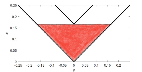
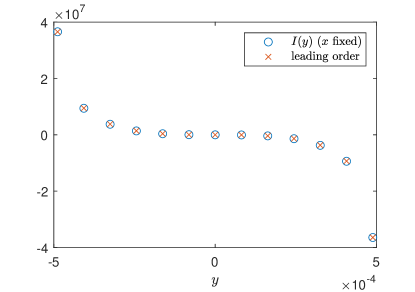
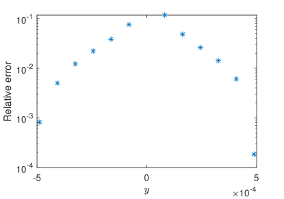
Figure 7: Top: Sub-region ${\rm IR}$, containing the singularity $k_{2}\to 0$. The region is represented after performing the change of variables $(k_{1},k_{2})\to(y,x)$. Bottom left: Some values of the integrand of (55) during the double loop of integration in the $x$ and $y$ variables. The circles are the full integrand integrated numerically, and the crosses are the leading order of the integrand in (55). In the plot, $x$ is fixed and $y$ varies from $-x$ to $x$. Note the magnitude of the integrand as the singular boundary is approached. Bottom right: relative error of the points in the left panel, in logaritmic scale.

$$|{g^{0}_{12}}^{\prime}|\simeq|{g^{1}_{02}}^{\prime}|\simeq m^{2}/{2k}\,,\qquad\Delta_{012}\simeq\frac{k^{2}}{\sqrt{x^{2}-y^{2}}}\,.$$ (53)

Using Eqs. (51)-(53), we finally obtain

$$R^{k}_{k(1+y),kx}+R^{k(1+y)}_{k,kx}\simeq 2k^{3}mx\left[2\frac{y^{2}}{x^{2}}\sqrt{x}+\frac{y}{x^{2}}(y^{2}-x^{2})\right]/\sqrt{x^{2}-y^{2}}\,.$$ (54)

Thus, Eq. (48) yields a contribution $\mathcal{I}_{C}(k)$ to the total $\mathcal{I}(k)$ (due to integration in region C):

$$\mathcal{I}_{\rm IR}(k) =8\pi k\int_{\rm IR}dx\,dy\;\left[-ak^{-2a}x^{-a}y\left(R^{k}_{k(1+y),kx}+R^{k(1+y)}_{k,kx}\right)\right]$$ (55)

$$=-16\pi ak^{-2a+4}m\int_{0}^{x_{\rm IR}}dx\int_{-x}^{x}dy\;x^{-a-1}\frac{2y^{3}\sqrt{x}+y^{2}(y^{2}-x^{2})}{\sqrt{x^{2}-y^{2}}}\,.$$

The first term of the integrand is dominating but it is an odd function of $y$ in a domain symmetric with respect to the origin, so its contribution is vanishing: this is the second cancellation, implying:

$$I_{\rm IR}(k) \sim-16\pi ak^{-2a+4}m\int_{0}^{x_{\rm IR}}dx\int_{-x}^{x}dy\;x^{-a-1}\frac{y^{2}(y^{2}-x^{2})}{\sqrt{x^{2}-y^{2}}}$$ (56)

$$=2\pi^{2}\frac{a}{4-a}mk^{-a}{k_{\rm IR}}^{-a+4}\,,$$

where $k_{\rm IR}$ is the (small) height of the red region in Fig. 7. For convergence of the integral we have to impose that $a<4$, and we notice that the contribution is positive.

The leading order of the integrand of Eq. (55) is tested numerically in the right panel of Fig. 7, leaving no doubt about its correctness.

7.2 Ultraviolet singularity

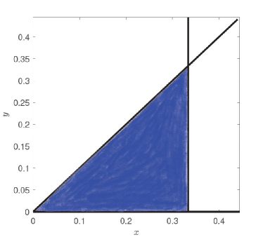
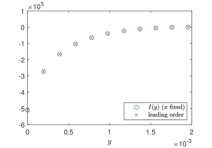
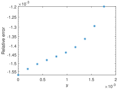
Figure 8: Top: Sub-region $D$, in the variables defined by Eq. (57). Bottom left: Some values of the integrand of (64) during the double loop of integration in the $x$ and $y$ variables. In the plot, $x$ is fixed and $y$ varies from $-x$ to $x$. Note the magnitude of the integrand as the singular boundary is approached. Bottom right: relative error of the points in the left panel, in logaritmic scale.

Let us focus on the region ${\rm UV}$, applying the following change of variables:

$$k_{1}=\frac{k}{x},\qquad k_{2}=\frac{k}{x}(1+y-x)\,,$$ (57)

for $x\ll 1$ and $y\in(0,x)$ . $1/x$ provides the largeness of $k_{1}$ and $k_{2}$, while $y=0$ corresponds to the singular line $k_{2}=k_{1}-k$, thereby allowing singular power expansions around the point $y=0$. Finally, $y=x$ corresponds to the line $k_{2}=k_{1}$. In the new variables, the region ${\rm UV}$ is represented in Fig. 8 (for a value $k_{\rm UV}=3k$). We have that the integrand of the UV contribution is given by

$$R^{0}_{12}f^{0}_{12}- R^{1}_{02}f^{1}_{02}-R^{2}_{01}f^{2}_{01}$$ (58)

$$\simeq \;-R^{k/x}_{k,k(1+y-x)/x}[n_{k}n_{k(1+y-x)/x}-n_{k/x}(n_{k}+n_{k(1+y-x)/x})]$$

$$-R^{k(1+y-x)/x}_{k,k/x}[n_{k}n_{k/x}-n_{k(1+y-x)/x}(n_{k}+n_{k/x})]$$

$$\simeq \;-a(x-y)k^{-2a}x^{a}\left[R^{k/x}_{k,k(1+y-x)/x}-R^{k(1+y-x)/x}_{k,k/x}\right]\,,$$

where $R^{0}_{12}$ has been neglected (subleading), and the first cancellation has taken place in the terms $f^{1}_{02}$ and $f^{2}_{01}$, expanded to first order in $x$ and $y$. Now, the two leading order contributions are given by the matrix elements satisfying the resonance conditions (${\rm IIb}$) and (${\rm IIIb}$), again the Induced Diffusion contributions, yielding respectively

$$m_{1}^{\star}\simeq-m\left(\frac{1}{\sqrt{x}}-\frac{y}{2x}\right)\,,\qquad m_{2}^{\star}\simeq-m\left(\frac{1}{\sqrt{x}}+1-\frac{y}{2x}\right)\,,$$ (59)

$$m_{1}^{\star}\simeq-m\left(\frac{1}{\sqrt{x}}+\frac{y}{2x}\right)\,,\qquad m_{2}^{\star}\simeq-m\left(\frac{1}{\sqrt{x}}-1+\frac{y}{2x}\right)\,,$$ (60)

which imply the leading order expressions

$$|V^{1}_{02}|^{2}/|{g^{2}_{13}}^{\prime}|\simeq\frac{2k^{2}m(x-y)^{2}}{x^{9/2}}+\frac{2k^{2}m(2x^{3}-4x^{2}y+3xy^{2}-y^{3})}{x^{5}}\,,$$ (61)

$$|V^{2}_{01}|^{2}/|{g^{2}_{01}}^{\prime}|\simeq\frac{2k^{2}m(x-y)^{2}}{x^{9/2}}-\frac{2k^{2}m(2x^{3}-4x^{2}y+3xy^{2}-y^{3})}{x^{5}}\,.$$ (62)

Plugging into the expression (48), with

$$\Delta_{012}\simeq\frac{k^{2}}{x^{2}}\sqrt{(2x-y)y}\,,$$ (63)

we finally obtain the following expression for the integrand:

$$-a(x-y)k^{-2a}x^{a} \left[R^{k/x}_{k,k(1+y-x)/x}-R^{k(1+y-x)/x}_{k,k/x}\right]$$ (64)

$$=-a(x-y)k^{-2a}x^{a}\frac{k^{3}}{x^{2}}\left[\frac{4k^{2}m}{x^{5}}(2x^{3}-4x^{2}y+3xy^{2}-y^{3})\right]\frac{x^{2}}{k^{2}\sqrt{(2x-y)y}}$$

$$=-4ak^{-2a+5}mx^{a-8}\left[(x-y)^{4}+x^{2}(x-y)^{2}\right]/\sqrt{(2x-y)y}\,.$$

This can be integrated analytically, giving the following result:

$$\mathcal{I}_{\rm UV}(k) =-32\pi ak^{-2a+4}m\int_{0}^{x_{\rm UV}}dx\int_{0}^{x}dy\;\frac{k^{2}}{x^{3}}\;x^{a-8}\left[(x-y)^{4}+x^{2}(x-y)^{2}\right]/\sqrt{(2x-y)y}$$ (65)

$$\simeq-14\pi^{2}\frac{a}{a-3}k^{-a+1}m\;k_{\rm UV}^{3-a}\,.$$

For convergence of the integral we must have that $a>3$, which along with the infrared condition results into the convergence segment $3<a<4$. Evidence of the correctness of the convergence condition $-3<a<4$ is given in the figures in the next Section, where the convergent integral is computed numerically.

8 Numerical computation of integrable singularities

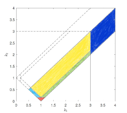
Figure 9: The five subregions of the kinematic box, where integration is performed (in the figure, $k=1$): region $\mathcal{R}_{1}$ (or ${\rm IR}$ in the main text) in red, region $\mathcal{R}_{2}$ in light blue, region $\mathcal{R}_{3}$ in green, region $\mathcal{R}_{4}$ in yellow, and region $\mathcal{R}_{5}$ (or ${\rm UV}$ in the main text) in blue. $\mathcal{R}_{1}$ contains the singularity for $k_{2}\to 0$; $\mathcal{R}_{2}$ and $\mathcal{R}_{3}$ contain the singularities due to a vanishing area of the interaction triangle with sides $k$, $k_{1}$ and $k_{2}$, which is at denominator in the integrand; $\mathcal{R}_{4}$ contains no singularities of the integrand; $\mathcal{R}_{5}$ is integrated over after a suitable change of coordinates that map the singularity of the integrand approaching infinity into the origin in the new coordinate system.

The five regions represented in Fig. 9, identified by the values of the two parameters $k_{\rm IR}$ and $k_{\rm UV}$, are treated separately. Just for numerical purpose, it is easier to consider these new regions, and then stich the results together to reconstruct the contributions of each of the regions in the main text. We recall that $k_{\rm IR}$ defines the height of the red region in Fig. 7 in the $k_{2}$ direction, and $k_{\rm UV}$ defines the lower boundary of the blue region in the $k_{1}$ direction. The singularities are integrated with the following procedure: the divergent leading order is subtracted to the integrand, giving a convergent difference that is integrated numerically. Subsequently, the exact analytical result of the integral of the subtracted part is added, ensuring convergence. The leading order in the regions $\mathcal{R}_{1}$ and $\mathcal{R}_{5}$ is given in the previous section, while the regions $\mathcal{R}_{2}$ and $\mathcal{R}_{3}$ are singular because of the $\Delta_{012}$ denominator at the boundary, i.e. the vanishing area of triangles formed by triads of collinear horizontal wave vectors.

In the code, the five terms are decomposed and integrated in the following form:

• Region $\mathcal{R}_{1}$:

  $$\mathcal{I}_{1}=\mathcal{L}+k^{2}\int_{0}^{k_{\rm IR}/k}dx^{\prime}\int_{-x}^{x}dy\left[J(x,y)-L(x,y)\right]\,,$$ (66)

  where

  $$J(x,y)=R^{k}_{k(1+y),kx}f^{k}_{k(1+y),kx}-R^{k(1+y)}_{k,kx}f^{k(1+y)}_{k,kx}-R^{kx}_{k,k(1+y)}f^{kx}_{k,k(1+y)}\,,$$

  $$L(x,y)=-2ak^{-2a+3}mx^{-a-1}\frac{2y^{3}\sqrt{x}+y^{2}(y^{2}-x^{2})}{\sqrt{x^{2}-y^{2}}}\,,\qquad\mathcal{L}=\frac{\pi}{4}\frac{a}{4-a}mk^{-a+1}k_{\rm IR}^{-a+4}\,.$$

• Region $\mathcal{R}_{2}$:

  $$\mathcal{I}_{2}=\int_{k/2}^{k-k_{\rm IR}}dk_{1}\left[\mathcal{L}(k_{1})+\int_{0}^{k_{\rm IR}}dx\left(J(x,k_{1})-L(x,k_{1})\right)\right]\,,$$ (67)

  where

  $$J(x,k_{1})=\frac{T^{k}_{k_{1},k-k1+x}-T^{k_{1}}_{k,k-k_{1}+x}-T^{k-k_{1}+x}_{k,k_{1}}}{\Delta_{k,k_{1},k-k_{1}+x}}\,,$$

  $$L(x,k_{1})=\frac{T^{k}_{k_{1},k-k_{1}}-T^{k_{1}}_{k,k-k_{1}}-T^{k-k_{1}}_{k,k_{1}}}{\sqrt{2kk_{1}(k-k_{1})x}}\,,\qquad\mathcal{L}(k_{1})=\left(T^{k}_{k_{1},k-k_{1}}-T^{k_{1}}_{k,k-k_{1}}-T^{k-k_{1}}_{k,k_{1}}\right)\frac{\sqrt{2k_{\rm IR}}}{\sqrt{kk_{1}(k-k_{1})}}\,,$$

  and the following definition was used:

  $$T^{0}_{12}=kk_{1}k_{2}|V^{0}_{12}|^{2}f^{0}_{12}/|{g^{0}_{12}}^{\prime}|\,.$$

• Region $\mathcal{R}_{3}$:

  $$\mathcal{I}_{3}=\int_{k+k_{\rm IR}}^{k_{\rm UV}}dk_{1}\left[\mathcal{L}(k_{1})+\int_{0}^{k_{\rm IR}}dx\left(J(x,k_{1})-L(x,k_{1})\right)\right]\,,$$ (68)

  where

  $$J(x,k_{1})=\frac{T^{k}_{k_{1},k1-k+x}-T^{k_{1}}_{k,k_{1}-k+x}-T^{k_{1}-k+x}_{k,k_{1}}}{\Delta_{k,k_{1},k_{1}-k+x}}\,,$$

  $$L(x,k_{1})=\frac{T^{k}_{k_{1},k_{1}-k}-T^{k_{1}}_{k,k_{1}-k}-T^{k_{1}-k}_{k,k_{1}}}{\sqrt{2kk_{1}(k_{1}-k)x}}\,,\qquad\mathcal{L}(k_{1})=\left(T^{k}_{k_{1},k_{1}-k}-T^{k_{1}}_{k,k_{1}-k}-T^{k_{1}-k}_{k,k_{1}}\right)\frac{\sqrt{2k_{\rm IR}}}{\sqrt{kk_{1}(k_{1}-k)}}\,,$$

• In region $\mathcal{R}_{4}$ the integrand is finite and integration is straightforward:

  $$\mathcal{I}_{4}=\int_{\mathcal{R}_{4}}dk_{12}\;(R^{0}_{12}f^{0}_{12}-R^{1}_{02}f^{1}_{02}-R^{2}_{01}f^{2}_{01})\,.$$ (69)

• Region $\mathcal{R}_{5}$:

  $$\mathcal{I}_{5}=\mathcal{L}+\int_{0}^{k/k_{\rm UV}}dx\int_{0}^{x}dy\left[J(x,y)-L(x,y)\right]\,,$$ (70)

  where

  $$J(x,y)=\left[R^{k}_{k/x,k(1+y-x)/x}f^{k}_{k/x,k(1+y-x)/x}-R^{k/x}_{k,k(1+y-x)/x}f^{k/x}_{k,k(1+y-x)/x}-R^{k(1+y-x)/x}_{k,k/x}f^{k(1+y-x)/x}_{k,k/x}\right]\frac{k^{2}}{x^{3}}\,,$$

  $$L(x,y)=-4ak^{-2a+5}mx^{a-8}\left[(x-y)^{4}+x^{2}(x-y)^{2}\right]/\sqrt{(2x-y)y}\,,\qquad\mathcal{L}=-\frac{7}{4}\pi\frac{a}{a-3}k^{-a+2}m\;k_{\rm UV}^{3-a}\,.$$

9 Numerical convergence and independence from the cuts

In Fig. 10 such numerical convergence is shown independently for each of the five regions. In region ${\rm UV}$ the two leading order contributions alone are integrated in Eq. (70), since there are subleading contributions whose integrand is divergent as well, hindering convergence. In the following, letting the position of the cut ($k_{\rm UV}$) vary, we will show that such term can indeed be neglected.

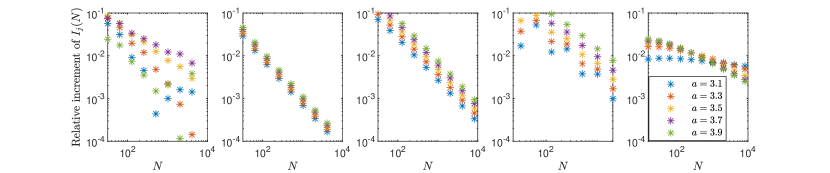
Figure 10: Test of convergence in each subregion of integration, as the number of gridpoints ($N$) increases. From left to right, the plots refer to regions from $\mathcal{R}_{1}$ to $\mathcal{R}_{5}$, respectively, and the plotted quantity is the absolute value of the relative increment of each contribution, as $N$ doubles (in log-log scale). All contributions appear to converge up to variations of at most $1\%$, for the largest numbers of points here considered.

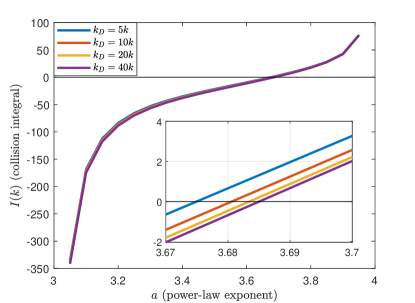
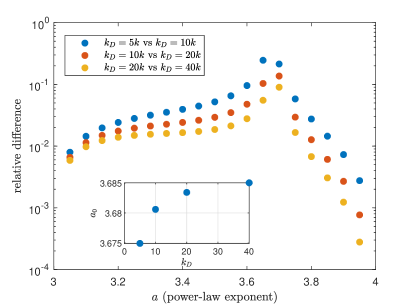
Figure 11: Left: Result of the integral as a function of the exponent $a$, as the cut at $k_{1}=k_{\rm UV}$ is sent toward infinity. The inset shows a zoomed region around the point where the integral vanishes. Right: Relative difference between the curves in the left panel, in logaritmic scale, giving evidence of convergence. In the inset, convergence of the stationary solution exponent (zero-crossing point in the left panel) is shown.

The width of the regions around $k_{2}=0$ is determined by the parameter $k_{\rm IR}$, while the cut at large $k$’s is performed at $k_{1}=k_{\rm UV}$. For the result to be general, it must be independent of the choice of $k_{\rm IR}$ and $k_{\rm UV}$, as long as they are finite numbers, $k_{\rm IR}$ being sufficiently small and $k_{\rm UV}$ sufficiently large. This has been checked. In Fig. 11 we show how convergence is reached as $k_{\rm UV}$ increases, as the neglected contribution in ${\rm UV}$ vanishes. Independence of the result upon variations of $k_{\rm IR}$ is even more robust (not shown here).