Operator Inference and Physics-Informed Learning of Low-Dimensional Models for Incompressible Flows

Abstract

Reduced-order modeling has a long tradition in computational fluid dynamics. The ever-increasing significance of data for the synthesis of low-order models is well reflected in the recent successes of data-driven approaches such as Dynamic Mode Decomposition and Operator Inference. With this work, we discuss an approach to learning structured low-order models for incompressible flow from data that can be used for engineering studies such as control, optimization, and simulation. To that end, we utilize the intrinsic structure of the Navier-Stokes equations for incompressible flows and show that learning dynamics of the velocity and pressure can be decoupled, thus leading to an efficient operator inference approach for learning the underlying dynamics of incompressible flows. Furthermore, we show the operator inference performance in learning low-order models using two benchmark problems and compare with an intrusive method, namely proper orthogonal decomposition, and other data-driven approaches.

37N10, 68T05, 76D05, 65F22, 93A15, 93C10

1 Introduction

The numerical solution of the incompressible Navier-Stokes equation is a demanding task in terms of computational effort and memory requirements. Reduced-order models can significantly decrease demands while maintaining a certain accuracy. One may well say that flow simulations have been a success story for the application of model reduction schemes as well as a driving force for the development of new approaches. For example, the popular methods of Proper Orthogonal Decomposition and Dynamic Mode Decomposition seem to have their origins in flow computations; see [45, 43]. On the other hand, the distinguished nonlinear and differential-algebraic structure of the semi-discrete incompressible Navier-Stokes has been attractive for the testing of extensions of standard system-theoretic approaches like Balanced Truncation (BT), LQG-BT, moment-matching, or polynomial expansions of the HJB equations; see [1, 8, 12, 22, 10]. Over the years, many applications and variants of POD for incompressible flows have been reported. We only mention particular works that include finite volume schemes, the use of supremizers, and pressure reconstruction [46, 47] that adaptively improve the bases for the use in optimal control [42], or works that address the algebraic constraint in different spatial discretizations [19] and refer to the numerous references therein. For an application of the Proper Generalized Decomposition (PGD), see [15].

Albeit the success of the projection-based methods such as POD, one of the significant drawbacks of these methods is that they require a discretized full-order model. It may be unavailable or a cumbersome task to obtain it. One may think of a scenario when a process is simulated using a black-box commercial solver. Hence, data-driven modeling has gained interest, aiming to determine reduced-order models directly using data that may be either obtained using a solver or in an experimental set-up. There exist vast literature on learning dynamical systems from data, and we review the most relevant literature to this work in what follows. Often referred to as system identification, the inference of models for linear time-invariant (LTI) systems has a long history with applications in control theory. One of the most relevant classical approaches is the eigenvalue realization algorithm, which was first proposed in [23] in the minimal realization set-up and then in [25] for system identification. This algorithm is based on the Hankel matrix using data from the system’s impulse response. For frequency domain data, several approaches were designed allowing rational interpolation of LTI transfer functions through, e.g., vector-fitting [20], Loewner approach [29, 34], and the so-called AAA algorithm [32].

On the other hand, nonlinear system identification requires an assumption on the structure of the non-linearity. Towards this, the Loewner framework has been extended to classes of nonlinear systems, especially bilinear and quadratic-bilinear systems in [3] and [17], respectively. Other identification methods are based on block-oriented nonlinear modeling, which defines systems as interconnections of an LTI block and static nonlinear blocks [16]. An example of these block-oriented modeling is the Wiener-Hammerstein systems, and many works have been dedicated to the identification of such systems, see, e.g., [11, 51, 44]. Lately, sparse identification has also emerged as a powerful technique [13]. The approach’s principle is to pick up a few nonlinear terms from a vast library of candidate nonlinear functions representing the dynamics of the system. However, it relies on the fact that the nonlinear terms that are important to represent the dynamics should be presented in the library. Another attractive data-driven method for nonlinear systems is based on the interpretation of dynamical systems via the Koopman operator, which readily applies to nonlinear systems. The identification is done by the so-called Dynamic Mode Decomposition (DMD). Curiously, DMD has initially been developed for low dimensional approximations of fluid dynamics [43]. Since then, it has seen various extensions such as extended DMD [49], kernel DMD [50], higher-order DMD [27]. Furthermore, it is intrinsically related to the Koopman operator analysis, see [31]. Moreover, DMD can be used to simultaneously identify an input operator [36, 37], and an output operator [2, 9]. Additionally in [18], the authors propose the DMD with control incorporation of quadratic-bilinear terms. We refer readers to [26] for a comprehensive monograph on this topic.

One often comes across scenarios where prior knowledge, such as governing equations of the process, is known. In these set-ups, however, the system parameters and discretization scheme are not known, but the underlying partial differential equations that govern the dynamics are known. Under these assumptions, the operator inference approach has emerged as a powerful tool to learn reduced-order models operators. It was first studied in [35], aiming at identifying nonlinear polynomial systems, which was later extended to general nonlinear systems [38, 7]. Moreover, recently, physics-informed neural network-based approaches have received a lot of attention, where one aims to utilize the known knowledge such as partial differential equations to build a model to solve nonlinear multi-physics problems, see, e.g., [41, 39, 40].

In this work, we focus on constructing models for incompressible flows. The dynamics of such a flow is, typically, given by the Navier-Stokes equations that comprise a differential equation and an algebraic equation. The algebraic equation enforces the incompressibility condition. Even though one may write down the equations, the discretization scheme and parameters such as the Reynolds number may be unknown. If the Reynolds is known, then physics-informed neural network for incompressible flow can be utilized that explicitly makes use of the known Navier-Stokes equations for incompressible flows, see [24]. However, the approach requires system parameters such as Reynolds numbers to be known, which may not be available, and the proposed methodology is valid for uncontrollable flows. Moreover, the proposed neural network has high-dimensional outputs that are the velocity and pressure in a given domain. Hence, the network can be computationally expensive for large-scale flows. But we know that the dynamics of large-scale dynamical systems typically lie in a low-dimensional subspace. With that aim, we propose a scheme to identifying reduced-order models for flows using data that incorporates the knowledge of Navier-Stokes equations for incompressible flows to learn reduced-order models from data; particularly, we discuss how to employ the operator inference approach proposed in [35] to incompressible flows governed by Navier-Stokes equations.

To this end, we discuss an application of the operator inference approach, proposed in [35] to build low-order models for incompressible flows. For this, we use the intrinsic structure of the semi-discrete Navier-Stokes equations and show that the learning dynamics of the velocity and pressure can be decoupled. As the main result, we present an efficient learning algorithm for modeling incompressible flows via a low-dimensional ordinary differential equation (ODE). In practice, it is a nontrivial task to extract such an underlying ODE from the model equations. As we will discuss, standard projection based approaches like POD may require corrections of the model and the projection basis and still suffer from systematic model errors caused by numerical inaccuracies. On the other hand, the tailored operator inference method for incompressible flows directly identifies an underlying ODE without being subjected to these theoretical and practical issues. Moreover, we show that in theory and under certain assumptions, the intrusive POD model converges to the learned model using the proposed non-intrusive method.

The rest of the manuscript is structured as follows. In Section 2, we introduce the spatially discretized incompressible Navier-Stokes equations in the velocity-pressure formulation and recall how to write the underlying ordinary differential equation for the velocity alone by eliminating the coupling with the pressure. In Section 3, we discuss an intrusive method (POD) to determine reduced-order models. In Section 4, we recap the operator inference approach, proposed in [35]. In Section 5, we tailor the operator inference approach for incompressible flows and show that intrusive and non-intrusive models converge under certain conditions. In Section 6, we discuss the case of inhomogeneity in the incompressibility constraints and its implications for the model reduction schemes. Finally, we present illustrative numerical studies in Section 7, and in the subsequent section, we conclude the paper with summarizing remarks and an outlook on future related research.

2 Navier-Stokes and its Equivalent Transformation as ODE

In this paper, we focus on the Navier-Stokes equations given in the partial differential form as follows:

$$\dfrac{\partial\mathfrak{v}}{\partial t} =-\mathfrak{v}\nabla\mathfrak{v}+\dfrac{1}{\texttt{Re}}\Delta\mathfrak{v}-\nabla\mathfrak{p}+f\quad \text{on}~{}\Omega,$$ (1)

$$\texttt{div}~{}\mathfrak{v} =g \text{on}~{}\Omega,$$

$$\dfrac{\partial\mathfrak{v}}{\partial t} =0 \text{on}~{}\partial\Omega,$$

$$\mathfrak{v} =\mathfrak{v}_{0} \text{for}~{}t=0,$$

where $\mathfrak{v}$ and $\mathfrak{p}$ are the velocity and pressure, respectively, and $\Omega$ and $\partial\Omega$ denote the domain and boundary of the domain, respectively; Re denotes the Reynolds number. We begin by presenting the differential algebraic equations (DAE), arising from the semi-discretization of the Navier-Stokes equation (1); that is,

$$\mathbf{E}_{11}\dot{\mathbf{v}}(t) =\mathbf{A}_{11}\mathbf{v}(t)+\mathbf{A}_{12}\mathbf{p}(t)+\mathbf{H}\left(\mathbf{v}\otimes\mathbf{v}\right)+\mathbf{f}(t),$$ (2a)

$$0 =\mathbf{A}_{12}^{\top}\mathbf{v}(t)+\mathbf{g}(t),\quad\mathbf{v}(0)=\mathbf{v}_{0},$$ (2b)

where $\mathbf{v}(t)\in\mathbb{R}^{n_{\mathbf{v}}}$, $\mathbf{p}(t)\in\mathbb{R}^{n_{\mathbf{p}}}$ are, respectively, the velocity and the pressure with $n_{\mathbf{v}}>n_{\mathbf{p}}$, and $\mathbf{E}_{11},\mathbf{A}_{11}\in\mathbb{R}^{n_{\mathbf{v}}\times n_{\mathbf{v}}}$, $\mathbf{A}_{12}\in\mathbb{R}^{n_{\mathbf{v}}\times n_{\mathbf{p}}}$, $\mathbf{f}(t)\in\mathbb{R}^{n_{\mathbf{v}}\times 1}$, $\mathbf{g}(t)\in\mathbb{R}^{n_{\mathbf{p}}\times 1}$; the initial condition for the velocity is denoted by $\mathbf{v}_{0}$. Furthermore, we assume that $\mathbf{E}_{11}$ and $\mathbf{A}_{12}^{\top}\mathbf{E}_{11}^{-1}\mathbf{A}_{12}$ are nonsingular matrices; hence, the system (2) is an index-2 linear system when $\mathbf{H}\equiv 0$. Additionally, we will suppose that the forcing terms are giving by

$$\mathbf{f}(t)=\mathbf{B}_{1}\mathbf{u}(t)\quad\text{and}\quad\mathbf{g}(t)\equiv 0,$$

where $\mathbf{u}(t)\in\mathbb{R}^{m}$ is an input vector and $\mathbf{B}_{1}\in\mathbb{R}^{n_{\mathbf{v}}\times m}$; we show how to handle the case when $\mathbf{g}(t)\neq 0$ in Section 6.

Next, we aim at transforming the DAE system (2) into an equivalent ODE system, which will be crucial in the analysis done in the rest of the paper.

Transformation of Navier-Stokes DAEs

Taking the time derivative of the algebraic conditions $\mathbf{A}_{12}^{\top}\mathbf{v}(t)=\mathbf{g}(t)=0$ $\forall t\geq 0$, implies that $\mathbf{A}_{12}^{\top}\dot{}\mathbf{v}(t)=0$ $\forall t\geq 0$. Then, we premultiply (2a) by $\mathbf{A}_{12}^{\top}\mathbf{E}_{11}^{-1}$ from the left-hand side, yielding:

$$0=\mathbf{A}_{12}^{\top}\mathbf{E}_{11}^{-1}\mathbf{A}_{11}\mathbf{v}(t)+\mathbf{A}_{12}^{\top}\mathbf{E}_{11}^{-1}\mathbf{A}_{12}\mathbf{p}(t)+\mathbf{A}_{12}^{\top}\mathbf{E}_{11}^{-1}\mathbf{H}(\mathbf{v}(t)\otimes\mathbf{v}(t))+\mathbf{A}_{12}^{\top}\mathbf{E}_{11}^{-1}\mathbf{f}(t).$$

With $\mathbf{S}:=\mathbf{A}_{12}^{\top}\mathbf{E}_{11}^{-1}\mathbf{A}_{12}$ being invertible, the pressure $\mathbf{p}$ can be expressed in terms of $\mathbf{v}$ and $\mathbf{f}$ as follows:

$$\mathbf{p}(t)=-\mathbf{S}^{-1}\mathbf{A}_{12}^{\top}\mathbf{E}_{11}^{-1}(\mathbf{A}_{11}\mathbf{v}(t)+\mathbf{H}(\mathbf{v}(t)\otimes\mathbf{v}(t))+\mathbf{f}(t)).$$ (3)

Substituting $\mathbf{p}(t)$ in (2a) from the above equation, we obtain an ODE for the velocity as follows:

$$\mathbf{E}_{11}\dot{}\mathbf{v}(t)=\Pi^{\top}\mathbf{A}_{11}\mathbf{v}(t)+\Pi^{\top}\mathbf{H}(\mathbf{v}(t)\otimes\mathbf{v}(t))+\Pi^{\top}\mathbf{f}(t),$$ (4)

where

$$\Pi^{\top}=\mathbf{I}-\mathbf{A}_{12}\mathbf{S}\mathbf{A}_{12}^{\top}\mathbf{E}_{11}^{-1}.$$ (5)

This leads to the important observation that although both the velocity and pressure are evolved and are coupled through the DAE (2), the DAE can be decoupled into an algebraic and differential part. Precisely, the evolution of the velocity over time can be given by the quadratic ODE (4), and there exists an algebraic equation that links the pressure and velocity given by (3).

Remark 1.

Equation (3) is often referred to as Pressure Poisson Equation, and the projector defined in (5) is called the discrete Leray Projector.

3 Projection-based Reduced-order Modeling for Navier-Stokes Equations

In this section, we discuss the construction of reduced-order models as surrogates for the large-scale DAEs in (2). To preserve the DAE structure, we consider block Galerkin projections. To that end, we aim at finding projection matrices $\mathbf{V}_{\mathbf{v}}\in\mathbb{R}^{n_{\mathbf{v}}\times r_{\mathbf{v}}}$ and $\mathbf{V}_{\mathbf{p}}\in\mathbb{R}^{n_{\mathbf{p}}\times r_{\mathbf{p}}}$ such that

$$\mathbf{v}(t)\approx\mathbf{V}_{\mathbf{v}}\mathbf{\widetilde{v}}(t)\quad\text{and}\quad\mathbf{p}\approx\mathbf{V}_{\mathbf{p}}\mathbf{\widetilde{p}}(t).$$

This leads to a reduced-order model that preserves the DAE structure:

$$\widetilde{\mathbf{E}}_{11}\mathbf{\dot{\widetilde{v}}}(t) =\widetilde{\mathbf{A}}_{11}\mathbf{\widetilde{v}}(t)+\widetilde{\mathbf{A}}_{12}\mathbf{\widetilde{p}}(t)+\widetilde{\mathbf{H}}\left(\mathbf{\widetilde{v}}\otimes\mathbf{\widetilde{v}}\right)+\mathbf{\widetilde{B}}_{1}\mathbf{u}(t),$$ (6a)

$$0 =\widetilde{\mathbf{A}}_{12}^{\top}\mathbf{\widetilde{v}}(t),$$ (6b)

where

$$\widetilde{\mathbf{E}}_{11} =\mathbf{V}_{\mathbf{v}}^{\top}\mathbf{E}_{11}\mathbf{V}_{\mathbf{v}}, \widetilde{\mathbf{A}}_{11} =\mathbf{V}^{\top}_{\mathbf{v}}\mathbf{A}_{11}\mathbf{V}_{\mathbf{v}},\quad\widetilde{\mathbf{A}}_{12}=\mathbf{V}_{\mathbf{v}}^{\top}\mathbf{A}_{12}\mathbf{V}_{\mathbf{p}},$$ (7)

$$\widetilde{\mathbf{H}} =\mathbf{V}_{\mathbf{v}}^{\top}\mathbf{H}\left(\mathbf{V}_{\mathbf{v}}\otimes\mathbf{V}_{\mathbf{v}}\right), \text{and}\quad\mathbf{\widetilde{B}}_{1} =\mathbf{V}_{\mathbf{v}}^{\top}\mathbf{B}_{1}.$$ (8)

The above reduced-order system can be obtained in a Galerkin projection framework using a holistic projection matrix as follows:

$$\mathbf{V}=\begin{bmatrix}\mathbf{V}_{\mathbf{v}}&\\ &\mathbf{V}_{\mathbf{p}}\end{bmatrix}.$$

POD projection bases

There exist several approaches to determine the projection matrices, see, e.g., [1, 8, 12, 22]. Here, we consider the case when the bases are determined using POD. In its basic form, an $r_{\mathbf{v}}$-dimensional $\mathbf{V}_{\mathbf{v}}$ projection matrix is determined using the $r_{\mathbf{v}}$ principal singular vectors of the snapshot matrix:

$$\mathbb{V}=\begin{bmatrix}\mathbf{v}(t_{0}),\mathbf{v}(t_{1}),\ldots,\mathbf{v}(t_{N})\end{bmatrix}.$$ (9)

One of many equivalent characterizations is the choice that minimizes the index

$$\|\mathbb{V}-\Pi_{r_{\mathbf{v}}}\mathbb{V}\|_{F}$$ (10)

over all projections $\Pi_{r_{\mathbf{v}}}$ of rank $k$ with $\mathbf{V}_{\mathbf{v}}\mathbf{V}_{\mathbf{v}}^{\top}$ being the minimizing projection.

In the context of the system (2), arising from the FEM or FVM discretization of the Navier-Stokes equations, the matrix $\mathbf{E}_{11}$ is a symmetric positive definite mass matrix that induces the discrete $L_{2}$ norm via

$$\|\mathbf{v}(t)\|_{\mathbf{E}_{11}}:=\sqrt{\mathbf{v}(t)^{\top}\mathbf{E}_{11}\mathbf{v}(t)}$$ (11)

and the corresponding index (10) as

$$\|\mathbf{L}_{\mathbf{E}_{11}}^{\top}(\mathbb{V}-\Pi_{k}\mathbb{V})\|_{F},$$ (12)

where $\mathbf{L}_{\mathbf{E}_{11}}$ is a factor of $\mathbf{E}_{11}$, i.e., $\mathbf{L}_{\mathbf{E}_{11}}\mathbf{L}_{\mathbf{E}_{11}}^{\top}=\mathbf{E}_{11}$. Hence, the $r_{\mathbf{v}}$-dimensional POD basis that minimizes the index (12) and respects the mass matrix, is given as

$$\mathbf{V}_{\mathbf{v}}:=\mathbf{L}_{\mathbf{E}_{11}}^{\top}\widetilde{\mathbf{V}}_{r_{\mathbf{v}}},$$ (13)

where $\widetilde{\mathbf{V}}_{r_{\mathbf{v}}}$ contains the $r_{\mathbf{v}}$ dominant left singular vectors of the matrix

$$\mathbf{L}_{E_{11}}^{-\top}\mathbb{V};$$

cp. [5, Lem. 2.5].

Remark 2.

In the true divergence-free case, i.e., if in the algebraic constraint (2b) $\mathbf{g}\equiv 0$, then the solution snapshots and the POD modes fulfill the constraint so that

$$\mathbf{A}_{12}^{\top}\mathbb{V}=0\quad\textnormal{and}\quad\mathbf{A}_{12}^{\top}\mathbf{V}_{\mathbf{v}}=0$$

and, thus, the reduced coefficients read $\widetilde{\mathbf{A}}_{12}=0$. Accordingly, the projected equations decouple and reduce to (6a). As a consequence, the reduced-order model obtained by POD has the following ordinary differential equation structure

$$\widetilde{\mathbf{E}}_{11}\mathbf{\dot{\widetilde{v}}}(t)=\widetilde{\mathbf{A}}_{11}\mathbf{\widetilde{v}}(t)+\widetilde{\mathbf{H}}\left(\mathbf{\widetilde{v}}\otimes\mathbf{\widetilde{v}}\right)+\mathbf{\widetilde{B}}_{1}\mathbf{u}(t),$$ (14)

where the algebraic conditions are automatically satisfied by the POD basis $\mathbf{V}_{\mathbf{v}}$.

Remark 3.

Even in the case when the snapshots are divergence-free, it may happen that the POD modes will not satisfy the constraints uniformly well as standard computational approaches for an SVD focus on the decomposition aspect. For a uniform accuracy of the decomposition, the accuracy of a singular vector can be inversely proportional to the associated singular value. For ODE systems, this inaccuracy is not an issue since the dominant modes are computed with high precision. For DAE systems, however, a failure in complying with the constraints introduces a systematic error. In the numerical examples later in the paper, we illustrate how the POD modes deviate from the actual subspace and how this limits the accuracy of POD for incompressible Navier-Stokes equations. A remedy for this could be the use of highly-accurate SVD computations [14] as it is available in LAPACK.

4 Operator Inference Approach

In the previous section, we discussed the projection-based model reduction based on POD. The approach requires the knowledge of the (semi-discretized in space) system matrices in (2), the so-called system realization. The reduced basis is obtained by compressing the time-domain snapshots of the system. Hence, the reduced-order model is typically constructed in the framework of Galerkin projection. Although this approach is effective in many set-ups, the assumption of having the full order model realization might lead to some practical limitations. In various instances, the dynamical system or a partial differential equation solver works as a black-box software, and the user has no access to the system realization. Hence, the authors in [35] have proposed an operator inference framework that aims at constructing reduced-order models directly using data without having access to the realization explicitly. In the following, we first give a brief overview of the operator inference approach[35] for ODEs. Let us consider a system of the form

$$\dot{}\mathbf{x}(t)=\mathbf{A}\mathbf{x}(t)+\mathbf{H}\left(\mathbf{x}(t)\otimes\mathbf{x}(t)\right)+\mathbf{B}\mathbf{u}(t),\quad\mathbf{x}(0)=\mathbf{x}_{0},$$ (15)

where $\mathbf{x}(t)\in\mathbb{R}^{n}$, $\mathbf{u}(t)\in\mathbb{R}^{m}$, and all the other system matrices are of appropriate size. We are interested in constructing a reduced-order model of the form:

$$\dot{\widehat{\mathbf{x}}}(t)=\widehat{\mathbf{A}}\widehat{\mathbf{x}}(t)+\widehat{\mathbf{H}}\left(\widehat{\mathbf{x}}(t)\otimes\widehat{\mathbf{x}}(t)\right)+\widehat{\mathbf{B}}\mathbf{u}(t),\quad\widehat{\mathbf{x}}(0)=\widehat{\mathbf{x}}_{0},$$ (16)

where $\widehat{\mathbf{x}}(t)\in\mathbb{R}^{r}$ such that $\mathbf{x}(t)\approx\mathbf{V}\widehat{\mathbf{x}}(t)$, where $\mathbf{V}$ is a projection matrix, and all the other system matrices are of appropriate size. We aim at constructing the reduced-order model (16) using the snapshots of $\mathbf{x}(t)$ at time steps $t_{0},t_{1},\ldots,t_{N}$ and input snapshots at the same time steps, i.e., $\mathbf{u}(t_{0}),\ldots,\mathbf{u}(t_{N})$. Now, we first collect these snapshots in matrices as follows:

$$\mathbf{X}=\begin{bmatrix}\mathbf{x}_{0},\ldots,\mathbf{x}_{N}\end{bmatrix},\quad\mathbf{U}=\begin{bmatrix}\mathbf{u}_{0},\ldots,\mathbf{u}_{N}\end{bmatrix},$$ (17)

where $\mathbf{x}_{i}:=\mathbf{x}(t_{i})$ and $\mathbf{u}_{i}:=\mathbf{u}(t_{i})$. Next, we determine dominant POD bases using the SVD of the matrix $\mathbf{X}$ and construct the projection matrix, denoted by $\mathbf{V}\in\mathbb{R}^{n\times r}$ using the $r$ dominant basis vectors. This allows us to compute the reduced state trajectory $\widehat{\mathbf{X}}=\mathbf{V}^{\top}\mathbf{X}$, where

$$\widehat{\mathbf{X}}:=\begin{bmatrix}\widehat{\mathbf{x}}(t_{0}),\ldots,\widehat{\mathbf{x}}(t_{N})\end{bmatrix}\quad\text{with}\quad\widehat{\mathbf{x}}(t_{i})=\mathbf{V}^{\top}\mathbf{x}_{i}.$$

Furthermore, we denote the derivative of $\widehat{\mathbf{x}}(t)$ at the time steps $t_{1}\ldots,t_{N}$ by $\dot{\widehat{\mathbf{x}}}(t_{0}),\ldots,\dot{\widehat{\mathbf{x}}}(t_{N})$, which can be approximated using the reduced trajectory $\widehat{\mathbf{x}}(t)$, see, e.g., [33, 28]. Next, we collect the time-derivative approximation of $\widehat{\mathbf{x}}(t)$ in a matrix as:

$$\dot{\widehat{\mathbf{X}}}=\begin{bmatrix}\dot{\widehat{\mathbf{x}}}(t_{0}),\ldots,\dot{\widehat{\mathbf{x}}}(t_{N})\end{bmatrix}.$$ (18)

We would like to point out that there exist several commercial software that make us available $\dot{}\mathbf{x}(t)$ as well. In such a case, an alternative way to compute the time-derivative of $\widehat{\mathbf{x}}(t)$ is by projecting $\dot{}\mathbf{x}(t)$ using the projection matrix $\mathbf{V}$, i.e., $\dot{\widehat{\mathbf{x}}}(t)=\mathbf{V}^{\top}\dot{}\mathbf{x}(t)$. However, in this paper, we consider the case where we do not have access to $\dot{}\mathbf{x}(t)$ and aim at estimating it using the data of $\widehat{\mathbf{x}}(t)$.

Having the projected data, we solve the following least-squares optimization problem to determine the operators of the reduced-order model (16):

$$\min_{\widehat{\mathbf{A}},\widehat{\mathbf{H}},\widehat{\mathbf{B}}}\left\|\dot{\widehat{\mathbf{X}}}-\begin{bmatrix}\widehat{\mathbf{A}},\widehat{\mathbf{H}},\widehat{\mathbf{B}}\end{bmatrix}\mathcal{D}\right\|,$$ (19)

where $\mathcal{D}=\begin{bmatrix}\widehat{\mathbf{X}}\\ \widehat{\mathbf{X}}\mathbin{\widetilde{\otimes}}\widehat{\mathbf{X}}\\ \mathbf{U}\end{bmatrix}$, and the product $\mathbin{\widetilde{\otimes}}$ is defined as

$$G\mathbin{\widetilde{\otimes}}G=\begin{bmatrix}g_{1}\otimes g_{1},\ldots,g_{N}\otimes g_{N}\end{bmatrix}$$ (20)

with $g_{i}$ being $i$-th column of the matrix $G\in\mathbb{R}^{n\times N}$. In many cases, we may find the matrix $\mathcal{D}$ to be ill-conditioned. There exist various possible ways to circumvent this issue, see, e.g., [52, 30]. In this paper, we use an SVD based approach; a similar approach is used in the context of DMD as well, e.g., in [4]. For this, we consider first the SVD of the matrix $\mathcal{D}$, denoted as follows:

$$\mathcal{D}=\mathcal{U}\Sigma\mathcal{V}^{\top}$$ (21)

Next, we neglect the singular values of the matrix $\mathcal{D}$ smaller than a given tolerance; hence, we can write

$$\mathcal{D}\approx\widetilde{\mathcal{U}}\widetilde{\Sigma}\widetilde{\mathcal{V}}^{\top},$$ (22)

where $\widetilde{\mathcal{U}}\in\mathbb{R}^{n+n^{2}+m\times r}$, $\widetilde{\Sigma}\in\mathbb{R}^{r\times r}$ and $\widetilde{\mathcal{V}}\in\mathbb{R}^{N\times r}$ and the number of singular values, larger than the tolerance, is $r$. As a result, we determine the matrices $\widehat{\mathbf{A}},\widehat{\mathbf{H}},\widehat{\mathbf{B}}$ as follows:

$$\begin{bmatrix}\widehat{\mathbf{A}},\widehat{\mathbf{H}},\widehat{\mathbf{B}}\end{bmatrix}=\dot{\widehat{\mathbf{X}}}\widetilde{\mathcal{V}}\widetilde{\Sigma}^{-1}\widetilde{\mathcal{U}}^{\top}.$$ (23)

We summarize all the necessary steps to obtain reduced-order models using the operator inference approach in Algorithm 1 with a slight modification, which is a regularization step.

Algorithm 1 Operator inference approach to learn low-dimensional models using data [35].

Input: Snapshots $\mathbf{x}(t)$ and $\mathbf{u}(t)$ at time steps $t_{0},t_{1},\ldots,t_{N}$, tol.

1:Determine projection matrix $\mathbf{V}\in\mathbb{R}^{n\times r}$, containing the dominant POD modes (or dominant singular vectors) of the matrix $\mathbf{X}=\begin{bmatrix}\mathbf{x}(t_{0}),\ldots,\mathbf{x}(t_{N})\end{bmatrix}$.

2:Compute the reduced trajectories $\widehat{\mathbf{x}}(t)$ at the same time steps:

$$\widehat{\mathbf{X}}:=\begin{bmatrix}\widehat{\mathbf{x}}(t_{0}),\ldots,\widehat{\mathbf{x}}(t_{N})\end{bmatrix},$$

where $\widehat{\mathbf{x}}(t_{i})=\mathbf{V}^{\top}\mathbf{x}(t_{i}),i\in\{0,\ldots,N\}$.

3:Approximate the time-derivative of $\widehat{\mathbf{x}}(t)$ using the reduced trajectory and collect them in a matrix as follows:

$$\dot{\widehat{\mathbf{X}}}:=\begin{bmatrix}\dot{\widehat{\mathbf{x}}}(t_{0}),\ldots,\dot{\widehat{\mathbf{x}}}(t_{N})\end{bmatrix}.$$

4:Compute the SVD of the matrix

$$\mathcal{D}=\begin{bmatrix}\widehat{\mathbf{X}}\\ \widehat{\mathbf{X}}\mathbin{\widetilde{\otimes}}\widehat{\mathbf{X}}\\ \mathbf{U}\end{bmatrix}=:\mathcal{U}\Sigma\mathcal{V}^{T},$$

where $\Sigma$ contains the singular values of the matrix $\mathcal{D}$ in the descending order.

5:Consider the singular values of the matrix $\mathcal{D}$ larger than tol. Let the number of singular values larger than tol be $\widetilde{r}$.

6:Compute the operators of the reduced-order model (16) as follows:

$$\begin{bmatrix}\widehat{\mathbf{A}},\widehat{\mathbf{H}},\widehat{\mathbf{B}}\end{bmatrix}=\dot{\widehat{\mathbf{X}}}\widetilde{\mathcal{V}}^{T}\widetilde{\Sigma}^{-1}\widetilde{\mathcal{U}}^{T},$$

where $\widetilde{\mathcal{U}}$ and $\widetilde{\mathcal{V}}$ are the first $\widetilde{r}$ columns of $\mathcal{U}$ and $\mathcal{V}$, respectively, and $\widetilde{\Sigma}$ is the principal $\widetilde{r}\times\widetilde{r}$ block of the matrix $\Sigma$.

Output: Operators: $\widehat{\mathbf{A}},\widehat{\mathbf{H}},\widehat{\mathbf{B}}$ of a reduced-order model, having the structure as (16).

Remark 4.

The tolerance, as an input to Algorithm 1, is a hyper-parameter. A larger tolerance yields a larger mismatch of the data fidelity term, whereas, for a smaller tolerance, the problem will become ill-conditioned. Therefore, one can employ the idea of an $L$-curve, discussed in [21] in the context of computed tomography. The $L$-curve analysis allows us to determine good tolerance that has a good compromise between the matching of data-fidelity term and making the problem well-conditioned.

5 Operator Inference for Navier-Stokes Equations

This section tailors the operator inference framework presented in the previous section to flow problems. We assume that the flow is incompressible, and the Navier-Stokes equations govern the underlying dynamics (2). With this assumption, consider the snapshots of the velocity and pressure vectors at the time steps $t_{0},t_{1},\dots,t_{N}$ and associate snapshot matrices as follows:

$$\mathbf{V}=\begin{bmatrix}\mathbf{v}(t_{0}),\mathbf{v}(t_{1}),\dots,\mathbf{v}(t_{N})\end{bmatrix}\quad\text{and}\quad\mathbf{P}=\begin{bmatrix}\mathbf{p}(t_{0}),\mathbf{p}(t_{1}),\dots,\mathbf{p}(t_{N})\end{bmatrix}$$ (24)

with the corresponding input matrix

$$\mathbf{U}=\begin{bmatrix}\mathbf{u}(t_{0}),\mathbf{u}(t_{1}),\dots,\mathbf{u}(t_{N})\end{bmatrix}.$$

Our goal is to construct reduced-order models that can predict the evolution of the velocity and pressure over time. We focus on constructing such models using only the velocity and pressures snapshot matrices $\mathbf{V}$ and $\mathbf{P}$ defined in (24) without having access to the discretized system (2) and its matrix realization. With this aim, let $\mathbf{V}_{\mathbf{v}}$ and $\mathbf{V}_{\mathbf{p}}$ be the dominant POD basis vectors of the velocity and pressure snapshot matrices $\mathbf{V}$ and $\mathbf{P}$, respectively. As a consequence, we can define the projected reduced velocity and pressure trajectories as follows:

$$\mathbf{\widehat{V}} =\begin{bmatrix}\mathbf{\widehat{v}}(t_{0})&\mathbf{\widehat{v}}(t_{1}),\dots,\mathbf{\widehat{v}}(t_{N})\end{bmatrix}=\mathbf{V}_{\mathbf{v}}^{\top}\mathbf{V},~{}~{}\text{and}$$ (25)

$$\mathbf{\widehat{P}} =\begin{bmatrix}\mathbf{\widehat{p}}(t_{0})&\mathbf{\widehat{p}}(t_{1}),\dots,\mathbf{\widehat{p}}(t_{N})\end{bmatrix}=\mathbf{V}_{\mathbf{p}}^{\top}\mathbf{P}.$$ (26)

Moreover, let $\dot{\widehat{\mathbf{v}}}(t_{i})$ denote the derivative of the reduced velocity $\widehat{\mathbf{v}}(t)$ at time $t_{i}$. It can be approximated using the reduced velocity trajectory $\widehat{\mathbf{v}}$ as given in (25). We collect the derivative information of $\mathbf{v}(t)$ in a matrix:

$$\mathbf{\dot{\widehat{V}}}=\begin{bmatrix}\dot{\widehat{\mathbf{v}}}(t_{0}),\ldots,\dot{\widehat{\mathbf{v}}}(t_{N})\end{bmatrix}.$$ (27)

Since the original system, arising from the Navier-Stokes discretization, has a quadratic DAE structure as (2), one could blindly consider a least-squares problem that yields a reduced DAE model (6), having the same structure as in (2). The matrices involved in defining (6) are the solution of the following optimization problem:

$$\min\limits_{\mathbf{\widehat{A}}_{11},\mathbf{\widehat{A}}_{12},\mathbf{\widehat{H}},\mathbf{\widehat{B}}_{1}}\left\|\begin{bmatrix}\mathbf{\widehat{A}}_{11}&\mathbf{\widehat{A}}_{12}&\mathbf{\widehat{H}}&\mathbf{\widehat{B}}_{1}\\ \mathbf{\widehat{A}}_{12}^{\top}&0&0&0\end{bmatrix}\mathbf{\widehat{X}}-\mathbf{\widehat{D}}\right\|^{2}_{F},$$

where

$$\mathbf{\widehat{X}}=\begin{bmatrix}\mathbf{\widehat{V}}\\ \mathbf{\widehat{P}}\\ \mathbf{\widehat{V}}{\mathbin{\widetilde{\otimes}}}\mathbf{\widehat{V}}\\ \mathbf{U}\end{bmatrix}\quad\text{and}\quad\mathbf{\widehat{D}}=\begin{bmatrix}\mathbf{\dot{\widehat{V}}}\\ 0\end{bmatrix}.$$

Note that so far, we have not used any additional information on the Navier-Stokes equations. One of the important observations we make is that the dynamics of the velocity in the Navier-Stokes equations is given independently of the pressure. Precisely, there is an underlying ODE for the velocity that completely describes its dynamics, see (4). This can also be seen when a reduced-order model is constructed using POD as described in Section 3 as long as the choice of the POD basis is divergence-free, i.e., $\mathbf{A}_{12}^{\top}\mathbf{V}_{\mathbf{v}}=0$. Moreover, the pressure and velocity are connected via an algebraic equation as shown in (3). Hence, it is conceivable to find an ODE for the reduced velocity $\widehat{\mathbf{v}}(t)$ as follows:

$$\dot{\widehat{\mathbf{v}}}(t)=\widehat{\mathbf{A}}_{\mathbf{v}}\mathbf{v}(t)+\widehat{\mathbf{H}}_{\mathbf{v}}\left(\mathbf{v}(t)\otimes\mathbf{v}(t)\right)+\widehat{\mathbf{B}}_{\mathbf{v}}\mathbf{u}(t),$$ (28)

and determine the algebraic equation relating pressure and velocity in a reduced space of the form

$$\widehat{\mathbf{p}}(t)=\widehat{\mathbf{A}}_{\mathbf{p}}\mathbf{v}(t)+\widehat{\mathbf{H}}_{\mathbf{p}}\left(\mathbf{v}(t)\otimes\mathbf{v}(t)\right)+\widehat{\mathbf{B}}_{\mathbf{p}}\mathbf{u}(t).$$ (29)

To that end, we can determine the involved operator to define (28) by the classical operator inference described in Section 4. For this, we aim at solving the following optimization problem:

$$\min_{\widehat{\mathbf{A}}_{\mathbf{v}},\widehat{\mathbf{H}}_{\mathbf{v}},\widehat{\mathbf{B}}_{\mathbf{v}}}\left\|\dot{\widehat{\mathbf{V}}}-\begin{bmatrix}\widehat{\mathbf{A}}_{\mathbf{v}},\widehat{\mathbf{H}}_{\mathbf{v}},\widehat{\mathbf{B}}_{\mathbf{v}}\end{bmatrix}\mathcal{D}\right\|_{F},$$ (30)

where $\mathcal{D}=\begin{bmatrix}\widehat{\mathbf{V}}\\ \widehat{\mathbf{V}}\mathbin{\widetilde{\otimes}}\widehat{\mathbf{V}}\\ \mathbf{U}\end{bmatrix}$. Similarly, we can solve the following optimization problem to find the operators of (31):

$$\min_{\widehat{\mathbf{A}}_{\mathbf{p}},\widehat{\mathbf{H}}_{\mathbf{p}},\widehat{\mathbf{B}}_{\mathbf{p}}}\left\|{\widehat{\mathbf{P}}}-\begin{bmatrix}\widehat{\mathbf{A}}_{\mathbf{p}},\widehat{\mathbf{H}}_{\mathbf{p}},\widehat{\mathbf{B}}_{\mathbf{p}}\end{bmatrix}\mathcal{D}\right\|_{F}.$$ (31)

As discussed in Section 4, the optimization problems (30) and (31) can be ill-conditioned; thus, we employ the similar remedy based on the SVD as discussed therein.

Next, we analyze the non-intrusive reduced model (28) with respect to the one obtained using an intrusive model. For this, we extend the result from [35, Sec 3.2] and show that the non-intrusive model (28) converges to the intrusive one. For this, we first make the following four assumptions:

Assumption 1.

The time-stepping scheme for the discretized model (2) is convergent in the $L_{2}$ norm for $\mathbf{v}$, i.e.,

$$\max_{i\in\{1,\dots,T/\Delta t\}}\|\mathbf{v}_{i}-\mathbf{v}(t_{i})\|_{2}\rightarrow 0\quad\text{as}\quad\Delta t\rightarrow 0.$$

Assumption 2.

The derivative approximation from the projected state converges to $\frac{d}{dt}\mathbf{\widehat{v}}(t_{N})$ as $\Delta t\rightarrow 0$.

Assumption 3.

The matrix data $\mathcal{D}=\begin{bmatrix}\widehat{\mathbf{V}}\\ \widehat{\mathbf{V}}\mathbin{\widetilde{\otimes}}\widehat{\mathbf{V}}\\ \mathbf{U}\end{bmatrix}$ has full column rank.

Assumption 4.

$\mathbf{V}_{\mathbf{v}}\in\mathbb{R}^{n\times r}$ is a divergence-free projected basis, i.e., $\mathbf{A}_{12}^{\top}\mathbf{V}_{\mathbf{v}}=0$.

Theorem 5.1.

Let Assumptions 1, 2, 3, and 4 hold. Let $\widetilde{\mathbf{E}}_{11}$, $\widetilde{\mathbf{A}}_{11}$, $\widetilde{\mathbf{H}}$ and $\mathbf{\widetilde{B}}_{1}$ be the reduced order ODE obtained by Galerkin projection as in (14) using the basis $\mathbf{V}_{\mathbf{v}}$. Then, for every $\varepsilon>0$, there exist an $r<n_{\mathbf{v}}$ and a $\Delta t>0$, such that

$$\|\widetilde{\mathbf{E}}_{11}^{-1}\widetilde{\mathbf{A}}_{11}-\mathbf{\widehat{A}}\|_{F}<\varepsilon,\quad\|\widetilde{\mathbf{E}}_{11}^{-1}\widetilde{\mathbf{H}}-\mathbf{\widehat{H}}\|_{F}<\varepsilon,\quad\text{and},\quad\|\widetilde{\mathbf{E}}_{11}^{-1}\mathbf{\widetilde{B}}_{1}-\mathbf{\widehat{B}}_{1}\|_{F}<\varepsilon.$$ (32)

Proof.

The proof follows the same lines as the one for [35, Theorem 1]. From Assumption 4, we know that the projected reduced model is of the quadratic ODE form (14), or equivalently,

$$\mathbf{\dot{\widetilde{v}}}(t)=\widetilde{\mathbf{E}}_{11}^{-1}\widetilde{\mathbf{A}}_{11}\mathbf{\widetilde{v}}(t)+\widetilde{\mathbf{E}}_{11}^{-1}\widetilde{\mathbf{H}}\left(\mathbf{\widetilde{v}}\otimes\mathbf{\widetilde{v}}\right)+\widetilde{\mathbf{E}}_{11}^{-1}\mathbf{\widetilde{B}}_{1}\mathbf{u}(t).$$ (33)

Let us denote $\widetilde{\mathcal{D}}=\begin{bmatrix}\widetilde{\mathbf{V}}\\ \widetilde{\mathbf{V}}\mathbin{\widetilde{\otimes}}\widehat{\mathbf{V}}\\ \mathbf{U}\end{bmatrix}$, where $\widetilde{\mathbf{V}}=\begin{bmatrix}\mathbf{\widetilde{v}}_{1},\mathbf{\widetilde{v}}_{2},\dots,\mathbf{\widetilde{v}}_{N}\end{bmatrix}$ denotes the data matrix assembling $N$ snapshots of the projected reduced model (33) and

$$\dot{\widetilde{\mathbf{V}}}=\begin{bmatrix}\frac{d}{dt}\mathbf{\widetilde{v}}(t_{1}),\frac{d}{dt}\mathbf{\widetilde{v}}(t_{2}),\dots,\frac{d}{dt}\mathbf{\widetilde{v}}(t_{N})\end{bmatrix}$$

is its right-hand side matrix. Hence, the reduced operators $\widetilde{\mathbf{E}}_{11}^{-1}\widetilde{\mathbf{A}}_{11}$, $\widetilde{\mathbf{E}}_{11}^{-1}\widetilde{\mathbf{H}}$ and $\widetilde{\mathbf{E}}_{11}^{-1}\mathbf{\widetilde{B}}_{1}$ represent one solution of the least-squares problem (30) for the data matrix $\widetilde{\mathcal{D}}$ and right-hand side matrix $\dot{\widetilde{\mathbf{V}}}$. Moreover, they represent the unique solution if the matrix $\widetilde{\mathcal{D}}$ has full rank.

Next, due to Assumption 1, notice that the projected velocities $\mathbf{\widehat{V}}$ are perturbations of the reduced velocities $\widetilde{\mathbf{V}}$, i.e., $\mathbf{\widehat{V}}=\widetilde{\mathbf{V}}+\delta\mathbf{V}$, and, for $\Delta t\rightarrow 0$ and the dimension $r$ increases, we have $\|\delta\mathbf{V}\|_{F}\rightarrow 0$, because the reduced model (33) is equivalent to the full-order ODE (4) in the POD basis of order $n_{\mathbf{v}}$. Also, Assumption 2 together with the limiting case $r=n_{\mathbf{v}}$ leads to $\frac{d}{dt}\mathbf{\widehat{v}}(t_{k})\rightarrow\frac{d}{dt}\mathbf{\widetilde{v}}(t_{k})$ as $r\rightarrow n_{\mathbf{v}}$, for $k=1,\dots,N$. As a consequence, the data matrix $\mathcal{D}$ and the approximated derivative information $\mathbf{\dot{\widehat{V}}}$ both can be interpreted as perturbation of $\widetilde{\mathcal{D}}$ and $\dot{\widetilde{\mathbf{V}}}$ respectively, i.e., $\mathcal{D}=\widetilde{\mathcal{D}}+\delta\mathcal{D}$ and $\mathbf{\dot{\widehat{V}}}=\dot{\widetilde{\mathbf{V}}}+\delta\dot{\mathbf{V}}$, with $\|\delta\mathcal{D}\|_{F}\rightarrow 0$ and $\|\delta\dot{\mathbf{V}}\|_{F}\rightarrow 0$ whenever $\Delta t\rightarrow 0$ and $r\rightarrow n_{\mathbf{v}}$. Hence, as presented in [7], this leads to the following asymptotic result for the least-squares problem:

$$\min_{\widehat{\mathbf{A}}_{\mathbf{v}},\widehat{\mathbf{H}}_{\mathbf{v}},\widehat{\mathbf{B}}_{\mathbf{v}}}\left[\lim\limits_{\begin{subarray}{c}\Delta t\rightarrow 0\\ r\rightarrow n_{\mathbf{v}}\end{subarray}}\left\|\dot{\widehat{\mathbf{V}}}-\begin{bmatrix}\widehat{\mathbf{A}}_{\mathbf{v}},\widehat{\mathbf{H}}_{\mathbf{v}},\widehat{\mathbf{B}}_{\mathbf{v}}\end{bmatrix}\mathcal{D}\right\|_{F}\right]=\min_{\widehat{\mathbf{A}}_{\mathbf{v}},\widehat{\mathbf{H}}_{\mathbf{v}},\widehat{\mathbf{B}}_{\mathbf{v}}}\left\|\dot{\widetilde{\mathbf{V}}}-\begin{bmatrix}\widehat{\mathbf{A}}_{\mathbf{v}},\widehat{\mathbf{H}}_{\mathbf{v}},\widehat{\mathbf{B}}_{\mathbf{v}}\end{bmatrix}\widetilde{\mathcal{D}}\right\|_{F}.$$

As a consequence, the pre-asymptotic case combined with Assumption 3 leads to the proof of the theorem. ∎

Theorem 5.1 shows that the identified operators converge to the POD projected operators as $r\rightarrow n_{\mathbf{v}}$. One particular limitation of this theorem is Assumption 4. Indeed, as mentioned in Remark 3, the SVD of the velocity snapshot matrix might generate POD modes that will not satisfy the algebraic constraints. This would result in intrusive velocity reduced-order models that are not fully independent of the pressure. On the other hand, the operator inferred model will still be a good approximation of the ODE velocity model (4). Another limitation of this theorem is that the least-squares problem in (30) can be ill-conditioned. The numerical remedy for that is the regularizer procedure from Remark 4. Although, in this case, Theorem 5.1 does not hold, it will be shown in Section 7 that the operator inference can still identify reduced-order models with very accurate state errors.

Remark 5.

If our goal is to learn a linear system as folllows:

$$\dot{\widehat{\mathbf{v}}}(t)=\widehat{\mathbf{A}}_{\mathbf{v}}\mathbf{v}(t)+\widehat{\mathbf{B}}_{\mathbf{v}}\mathbf{u}(t),$$ (34)

that captures the dynamics of the nonlinear Navier-Stokes equations as close as possible, in the above described operator inference approach, we set $\widehat{\mathbf{H}}\equiv 0$. Such a linear model can be learned by solving the above least-squares problem

$$\min_{\widehat{\mathbf{A}}_{\mathbf{v}},\widehat{\mathbf{B}}_{\mathbf{v}}}\left\|\dot{\widehat{\mathbf{V}}}-\begin{bmatrix}\widehat{\mathbf{A}}_{\mathbf{v}},\widehat{\mathbf{B}}_{\mathbf{v}}\end{bmatrix}\mathcal{D}\right\|_{F},\quad\text{where $\mathcal{D}=\begin{bmatrix}\widehat{\mathbf{V}}\\ \mathbf{U}\end{bmatrix}$.}$$ (35)

6 Inhomogeneities in the Continuity Equation

In case $\mathbf{A}_{12}^{\top}\mathbf{v}(t)-\mathbf{g}(t)=0$ and $\mathbf{g}\not\equiv 0$, we decompose the state $\mathbf{v}$ as $\mathbf{v}(t)=\mathbf{v}_{\top}(t)+\mathbf{v}_{\perp}(t)$, where $\mathbf{v}_{\top}(t)\in\ker\mathbf{A}_{12}^{\top}$ that can be defined as a solution to an ODE, and $\mathbf{v}_{\perp}(t)$ is an element of the complement of $\ker\mathbf{A}_{12}^{\top}$. This is typically done in the literature to compute projection-based reduced-order models in such cases, see, e.g., [22, 1]. An advantage of this decomposition is that we can employ model reduction schemes developed for the homogeneous case, i.e., $\mathbf{A}_{12}^{\top}\mathbf{v}(t)=0$. With the discrete Leray projection as in (5), one has

$$\mathbf{v}(t)=\Pi\mathbf{v}(t)+(\mathbf{I}-\Pi)\mathbf{v}(t)=:\mathbf{v}_{\top}(t)+\mathbf{v}_{\perp}(t)$$ (36)

with the remainder part given as

$$\mathbf{v}_{\perp}(t)=-\mathbf{E}_{11}^{-1}\mathbf{A}_{12}(\mathbf{A}_{12}^{\top}\mathbf{E}_{11}^{-1}\mathbf{A}_{12})^{-1}\mathbf{g}(t).$$ (37)

Assume that $\mathbf{g}(t)=\mathbf{B}_{\perp}\mathbf{u}_{\perp}(t)$ with $\mathbf{u}_{\perp}(t)\in\mathbb{R}$; thus, we can write $\mathbf{v}_{\perp}(t)=\mathbf{S}_{\perp}\mathbf{u}_{\perp}(t)$. In this case, the pressure $\mathbf{p}$ is defined via

$$\mathbf{p}(t)=-\mathbf{S}^{-1}(\mathbf{A}_{12}^{\top}\mathbf{E}_{11}^{-1}\mathbf{A}_{11}\mathbf{v}(t)+\mathbf{A}_{12}^{\top}\mathbf{E}_{11}^{-1}\mathbf{H}(\mathbf{v}(t)\otimes\mathbf{v}(t))+\mathbf{A}_{12}^{\top}\mathbf{E}_{11}^{-1}\mathbf{f}(t)-\mathbf{B}_{\perp}\dot{}\mathbf{u}_{\perp}(t))$$

and the ODE (4) can be formulated for $\mathbf{v}_{\top}$ via

$$\mathbf{E}_{11}\dot{\mathbf{v}}_{\top}(t) =\mathbf{A}_{11}\mathbf{v}_{\top}(t)+\mathbf{H}(\mathbf{v}_{\top}(t)\otimes\mathbf{v}_{\top}(t))+\mathbf{N}\mathbf{v}_{\top}(t)\mathbf{u}_{\perp}(t)$$ (38)

$$\quad+\mathbf{H}\left(\mathbf{S}_{\perp}\otimes\mathbf{S}_{\perp}\right)\mathbf{u}_{\perp}^{2}(t)+\mathbf{A}_{12}\mathbf{p}(t)+{\mathbf{f}}(t),$$

where $\mathbf{N}=\mathbf{H}\left(\mathbf{I}\otimes\mathbf{S}_{\perp}+\mathbf{S}_{\perp}\otimes\mathbf{I}\right)$.

Remark 6.

Because $\Pi\dot{\mathbf{v}}_{\perp}(t)\equiv 0$, one can show that $\dot{\mathbf{v}}_{\perp}$ does not occur in (38); cp. [22, Sec. 6].

For a projection based reduction as described in Section 3, the following considerations are relevant:

• If $\mathbf{g}\equiv 0$ and the basis $\mathbf{V}$ is divergence-free, i.e. $\mathbf{A}_{12}^{\top}\mathbf{V}=0$, then $\mathbf{\widetilde{A}}_{12}=0$ and the projected equation (6a) recovers the corresponding projection of (4).

• If $\mathbf{g}\neq 0$ and, thus, the corresponding basis $\mathbf{V}$ is not divergence-free when they are computed using the original velocity snapshots, i.e.,

  $$\mathbf{V}=\begin{bmatrix}\mathbf{v}(t_{0}),\mathbf{v}(t_{1}),\dots,\mathbf{v}(t_{N})\end{bmatrix},$$ (39)

  we first need to compute a divergence-free basis on the base of $\Pi\mathbf{V}$ and $\mathbf{v}_{\perp}(t)$ and apply the projection procedure to the corrected full order model (38).

Note that the resulting ODE equation has some additional terms if compared (6a); these are a bilinear term and square term of the input. But for a special case $\mathbf{u}_{\perp}(t)\equiv\texttt{const}$, the bilinear term can be merged into the linear term, and the square input term becomes a constant. Furthermore, we mention that if the numerical realization of $\Pi$ is impossible or too costly, one may apply empirically divergence-free bases obtained by a projection defined by snapshots of the discrete pressure gradient

$$\mathbb{P}:=\begin{bmatrix}\mathbf{A}_{12}\mathbf{p}(t_{0}),\mathbf{A}_{12}\mathbf{p}(t_{1}),\ldots,\mathbf{A}_{12}\mathbf{p}(t_{N})\end{bmatrix}.$$ (40)

Let $\mathbf{Q}_{N}$ be an orthogonal basis of $\mathop{\mathrm{span}}\left(\mathbb{P}\right)$. Then, for the projection $\widetilde{\Pi}:=\mathbf{I}-\mathbf{Q}_{N}\mathbf{Q}_{N}^{\top}$, it holds that $\widetilde{\Pi}\mathbb{P}=0$. Consequently, for a basis $\widetilde{\mathbf{V}}_{\mathbf{v}}=\widetilde{\Pi}\widetilde{\mathbf{V}}_{\mathbf{v}}$, we have $\widetilde{\mathbf{V}}_{\mathbf{v}}^{\top}\mathbf{A}_{12}\mathbf{p}(t_{k})=0$ at all snapshot locations $t_{k}$. Accordingly, for a Galerkin projection of (38) by $\widetilde{\mathbf{V}}_{\mathbf{v}}=\widetilde{\Pi}\widetilde{\mathbf{V}}_{\mathbf{v}}$, one may well assume that $\widetilde{\mathbf{A}}_{12}=0$, since this condition holds at all data points.

When the exact projection $\Pi$ is known and $\mathbf{u}_{\perp}\equiv\texttt{const}$, the approximation of the full state is defined as

$$\mathbf{v}(t)\approx\widetilde{\mathbf{V}}_{\mathbf{v}}^{\top}\widehat{\mathbf{v}}(t)+\mathbf{v}_{\perp}(t):=\widetilde{\mathbf{V}}_{\mathbf{v}}^{\top}\widehat{\mathbf{v}}(t)+(\mathbf{I}-\widetilde{\Pi})\mathbf{v}(t_{0})\approx\widetilde{\mathbf{V}}_{\mathbf{v}}^{\top}\widehat{\mathbf{v}}(t)+\mathbf{Q}_{N}\mathbf{Q}_{N}^{\top}\mathbf{v}(t_{0}),$$ (41)

where the reduced state $\widehat{\mathbf{v}}$ solves the projected (and corrected) equations (38) with $\widetilde{\mathbf{A}}_{12}$ set to zero; cp. also (14).

The preceding considerations are only relevant for projection-based methods from Section 3. These modifications are not necessary when a model is learned using data. It is based on the fact that the dynamics of velocity can be governed by an ODE regardless of whether the velocity satisfies divergence-free constraint or not. To elaborate more on it, we consider the algebraic equations as follows:

$$\mathbf{A}_{12}^{\top}\mathbf{v}(t)+\mathbf{B}_{\perp}\mathbf{u}_{\perp}(t)=0,$$ (42)

implying

$$\mathbf{A}_{12}^{\top}\dot{}\mathbf{v}(t)+\mathbf{B}_{\perp}\dot{}\mathbf{u}_{\perp}(t)=0.$$ (43)

Next, we substitute the equation for $\dot{}\mathbf{v}(t)$ from (2), we get

$$0=\mathbf{A}_{12}^{\top}\mathbf{E}_{11}^{-1}\mathbf{A}_{11}\mathbf{v}(t)+\mathbf{A}_{12}^{\top}\mathbf{E}_{11}^{-1}\mathbf{A}_{12}\mathbf{p}(t)+\mathbf{A}_{12}^{\top}\mathbf{E}_{11}^{-1}\mathbf{H}(\mathbf{v}(t)\otimes\mathbf{v}(t))+\mathbf{A}_{12}^{\top}(\mathbf{E}_{11}^{-1}\mathbf{f}(t)+\mathbf{B}_{2}\dot{}\mathbf{u}_{\perp}(t)).$$ (44)

With $\mathbf{S}:=\mathbf{A}_{12}^{\top}\mathbf{E}_{11}^{-1}\mathbf{A}_{12}$ being invertible, the pressure $\mathbf{p}$ can be expressed in terms of $\mathbf{v}$ and $\mathbf{f}$ as follows:

$$\mathbf{p}(t)=-\mathbf{S}^{-1}\mathbf{A}_{12}^{\top}\mathbf{E}_{11}^{-1}(\mathbf{A}_{11}\mathbf{v}(t)+\mathbf{H}(\mathbf{v}(t)\otimes\mathbf{v}(t))+\mathbf{f}(t))-\mathbf{S}^{-1}\mathbf{A}_{12}^{\top}\mathbf{B}_{2}\dot{}\mathbf{u}_{\perp}(t).$$ (45)

Substituting $\mathbf{p}(t)$ in (2a) from the above equation, we obtain an ODE for the velocity as follows:

$$\mathbf{E}_{11}\dot{}\mathbf{v}(t)=\Pi^{\top}\mathbf{A}_{11}\mathbf{v}(t)+\Pi^{\top}\mathbf{H}(\mathbf{v}(t)\otimes\mathbf{v}(t))+\Pi^{\top}\mathbf{f}(t)-\mathbf{A}_{12}\mathbf{S}^{-1}\mathbf{A}_{12}^{\top}\mathbf{B}_{\perp}\dot{}\mathbf{u}_{\perp}(t).$$ (46)

This illustrates that there exists an underlying ODE for the velocity, even in the inhomogeneous case. Hence, we can determine the underlying ODE by employing the proposed operator inference approach, discussed in Section 5 with a slight modification. This is to include learning the operator for the derivative of the input $\mathbf{u}_{\perp}$. This is one of the significant advantages of the non-intrusive method over the intrusive POD method.

Remark 7.

One may argue that intrusive approaches can be applied to (46), but this is highly undesirable since it requires the explicit computation of matrices such as $\Pi^{\top}\mathbf{A}_{11}$ to determine projected reduced matrices. Moreover, some matrices, e.g., $\Pi^{\top}\mathbf{A}_{11}$ may lose sparsity, thus making intrusive model reduction computationally very expensive.

7 Numerical experiments

In this section, we illustrate the efficiency of the proposed method using numerical experiments and compare with the intrusive POD method and the data-driven method DMD. Precisely, the following methodologies are compared:

• OpInf: the proposed operator inference from Section 5,

• OpInf_lin: its linear variant described in Remark 5,

• POD: intrusive model reduction based on POD, see Section 3,

• DMD: classical DMD approach, see [48, Algorithm 1],

• DMDc: DMD with control, see [36, Algorithm 3.4]), and

• DMDquad: DMD with quadratic term and control, see [18, Section 3.2].

Moreover, below, we provide some technical information that applies to the construction of the surrogate models and the integration of the reduced systems:

• POD, OpInf and OpInf_lin surrogate models are simulated using the Python routine odeint from scipy.integrate.

• To employ the operator inference approach, we require the time-derivative approximation of $\mathbf{\widehat{v}}(t)$. This is obtained using the reduced trajectory $\widehat{\mathbf{v}}(t)$ by employing a fourth-order Runge-Kutta scheme.

• The DMD procedures are applied to the projected velocity trajectories (25) and then lifted using the POD basis.

• We assume that the POD surrogate models are pure ODE models as (14), i.e., $\mathbf{\widetilde{A}}_{12}=0$ in (7). For that we apply the necessary corrections as indicated by the theory laid out in Section 6. However, since this is not in the scope of the standard POD approach, we will not take particular measures against the error introduced by inaccuracies in the SVD (cp. Remark 3).

The code and the raw data is made available as mentioned in Figure 14.

7.1 A low-order demo example

In order to illustrate the proposed approach, we create a low-order random demo example of the form (2). We have generated it using the seed $0$ with $n_{\mathbf{v}}=4$ and $n_{\mathbf{p}}=1$. We construct the data for velocity and pressure using an input $u(t)=\sin(2t)e^{-0.05t}$ with zero initial condition. Next, we learn surrogate models using OpInf, DMD, DMDc, and DMDquad. We set the tolerance $\texttt{tol}=10^{-4}$ for the SVD (step 5 of Algorithm 1). In Figure 1, we compare the time-domain simulations of the original and inferred model using OpInf. Moreover, we plot the mean-absolute error of the velocity of the original and various inferred models in Figure 2. We observe that OpInf learns the best model among the considered approaches that capture the dynamics of the given data. DMD approaches that aim to learn a linear model fail to capture the dynamics; however, DMD with quadratic observers improves the model as one can expect.

Figure 1: A comparison of the velocity of the original model and inferred model using OpInf.

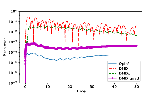
Figure 2: A comparison of the velocity obtained from the original model and inferred models using various approaches.

7.2 Navier-Stokes examples

We consider two test cases modeled by incompressible Navier-Stokes equations; namely, the lid driven cavity and cylinder wake, to illustrate the performance and highlight certain properties of the non-intrusive schemes. Both examples consider two-dimensional flows. For the spatial discretization, we use Taylor-Hood elements with piece-wise quadratic ansatz functions for the velocities and piece-wise linear ansatz functions for the pressure on a triangulation; see Figure 3 for an illustration of the setup.

As described, e.g., in [6], a spatial discretization of the problems leads to a system of the form (cp. (2))

$$\mathbf{E}_{11}\dot{\mathbf{v}}(t) =\mathbf{A}_{11}\mathbf{v}(t)+\mathbf{A}_{12}\mathbf{p}(t)+\mathbf{H}\left(\mathbf{v}(t)\otimes\mathbf{v}(t)\right)+\mathbf{f}(t),$$ (47a)

$$0 =\mathbf{A}_{12}^{\top}\mathbf{v}(t)+\mathbf{g}(t),$$ (47b)

$$y_{\mathbf{v}}(t) =\mathbf{C}_{\mathbf{v}}\mathbf{v}(t),$$ (47c)

$$y_{\mathbf{p}}(t) =\mathbf{C}_{\mathbf{p}}\mathbf{p}(t),$$ (47d)

where $y_{\mathbf{v}}$ and $y_{\mathbf{p}}$ denotes characteristic outputs that is derived from the state $\mathbf{v}$ and $\mathbf{p}$ via a linear map, respectively; cp. [6, Ch. 8].

Figure 3: An illustration of the computational domains of the driven cavity flow (above) and and flow around a cylinder (below), and example discretizations of the respective domains.

The driven cavity example describes an internal flow in a cavity that is driven by a moving lid (depicted by $\Gamma_{0}$ in Figure 3) modeled by a Dirichlet boundary condition for the tangential component of the velocity. The resulting semi-discrete system is as in (47) with $\mathbf{g}(t)\equiv 0$. On the other hand, the cylinder wake example models flow through a channel with a round obstacle in between. The flow is induced by a strongly imposed parabolic flow profile at the inlet (depicted by $\Gamma_{0}$ in Figure 3). The corresponding semi-discrete model is in the form of (47) with $\mathbf{g}(t)\equiv\mathop{const}$.

7.2.1 Numerical setup and computation of the snapshots

As for the discretization of the time dimension, we apply an implicit-explicit Euler scheme – i.e., an explicit treatment of the nonlinear term and implicit treatment of the linear term and, in particular, the constraint equation in (47) – on an equidistant grid. For the initial value, we use the solution of the corresponding steady-state Stokes problem.

To probe the accuracy of the discretization and, thus, the reliability of the snapshots and the resulting reduced-order models, we compute the resulting discrete approximation of the velocities $v$

$$\int_{0}^{T}\|v(t)\|_{L^{2}(\Omega)}dt,$$ (48)

where $T$ is the end time (see Table 1) and $\Omega$ is the domain of the problems, and compare it to the corresponding approximation based on a finer spatial grid and a high-accuracy time integration scheme with step-size control applied to the ODE formulation (4). As indicated by the numbers presented in Table 2, the error in the spatial discretization is dominating, so that the linear convergence of the time integration scheme only occurs on the finest triangulation.

Parameter	driven cavity	cylinder wake
Reynolds number	500	60
state dimensions $(n_{\mathbf{v}},n_{\mathbf{p}})$	(3042,441)	(9356,1289)
time interval	[0, 6]	[0, 2]
number of timesteps	512	512
number of snapshots	513	513
order of discretized model (47)	3042	5812

Table 1: The parameters of the numerical setups.

driven cavity

$n_{\mathbf{v}}$/ number of timesteps	$256$	$512$	$1024$
$722$	$-0.0988$	$-0.0992$	$-0.0993$
$3042$	$-0.0292$	$-0.0299$	$-0.0303$
$6962$	$0.0015$	$0.0007$	$0.0003$

cylinder wake

$n_{\mathbf{v}}$/ number of timesteps	$512$	$1024$	$2048$
$5812$	$-0.0022$	$-0.0025$	$-0.0026$
$9356$	$-0.0002$	$-0.0005$	$-0.0006$
$19468$	$0.0005$	$0.0002$	$0.0001$

Table 2: The difference in the numerical approximation of the norm of the computed velocity to the approximation on the finest spatial discretization with a high-accuracy time integration scheme.

Remark 8.

For the large-scale Navier-Stokes examples, DMDquad produced only unstable models; therefore, the results will not be reported.

7.2.2 Example 1: driven cavity

Here, we report the numerical experiments conducted for the driven cavity example. We consider the full-order model (FOM) semi-discretized in space of order $n_{\mathbf{v}}=3042$. To infer models, $513$ velocity snapshots are generated in the interval $[0,6]$ equally spaced in time using the implicit-explicit Euler scheme. It is again worth noticing that, for this example, $\mathbf{g}(t)\equiv 0$. As a consequence, the velocity snapshot matrix $\mathbf{V}$ satisfies the algebraic constraints, i.e., $\mathbf{A}_{12}^{\top}\mathbf{V}=0$. Then, the POD basis $\mathbf{V}_{\mathbf{v}}$ was constructed using the SVD of the snapshot matrix $\mathbf{V}$. Figure 4 depicts the decay of the singular values of the snapshot matrix and shows how much the algebraic conditions are satisfied if the POD basis is increased, i.e.,

$$\dfrac{\|\mathbf{A}_{12}^{\top}\mathbf{V}_{\mathbf{v}}\|_{F}}{\|\mathbf{V}_{\mathbf{v}}\|_{F}},$$

as function of the reduced order $r_{\mathbf{v}}$. As expected, the POD basis does not satisfy the algebraic constraints if a larger order for the reduced model is chosen. Consequently, for high orders of the reduced models, the POD bases are not entirely divergence-free, leading to surrogate models that have a non-neglectable influence of the pressure. Ideally, these POD bases should be divergence-free, but in standard implementations in Python and MATLAB, singular vectors corresponding to smaller singular values are computed with low accuracy; cp. Remark 3.

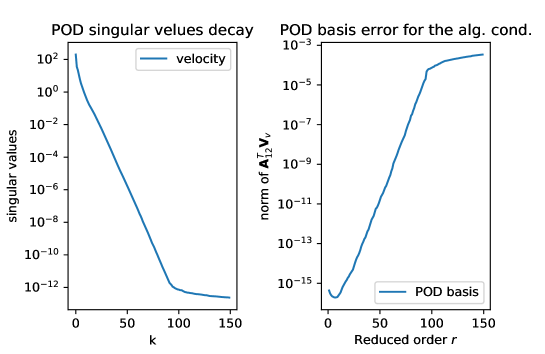
Figure 4: driven cavity: Decay of singular values and POD basis error for algebraic conditions.

We infer reduced-order models of order $r_{\mathbf{v}}=30$ using OpInf, OpInf_lin, POD, DMD, and DMDc. As mentioned in Remark 4, the least-squares problem arising in OpInf can be ill-conditioned; thus, the choice of tol in step 5 of Algorithm 1 plays a crucial role. Hence, for different tolerances in the range of $[10^{-11},10^{-6}]$, Figure 5 shows the L-curve, i.e., for each given tol, a scatter plot between the least-squares error and the norm of the least-squares solution. Using the L-curve criterion, we set the tolerance as $\texttt{tol}=10^{-7}$. Figure 6 depicts the time-domain simulation of some observed trajectories for order $r_{\mathbf{v}}=30$. It also shows the error $\|\mathbf{v}_{\texttt{FOM}}(t)-\mathbf{\widehat{v}}_{\texttt{ROM}}(t)\|_{F}^{2}$ committed by the different surrogate models. Surprisingly, although the FOM had an intrinsic nonlinear behavior, OpInf, OpInf_lin and DMDc have a similar performance on this model. These three methodologies outperform DMD and POD. Additionally, by solving the least-squares problem (31), one obtains the OpInf reduced model for the pressure. The time-domain evolution of the pressure for the FOM and OpInf models are depicted in Figure 7 as well as the approximation error.

Figure 5: driven cavity: L-curve for $r_{\mathbf{v}}=30$

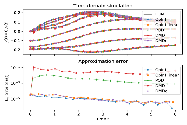
Figure 6: driven cavity: A comparison of time-domain simulations of the original and reduced-order models for $r_{\mathbf{v}}=30$.

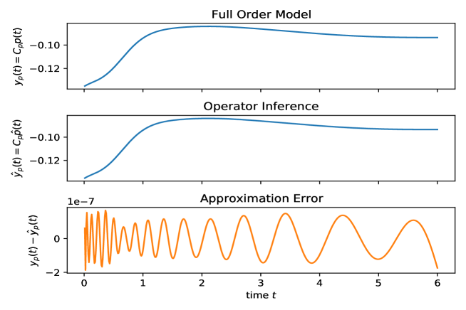
Figure 7: driven cavity: Time-domain evolution of the observed pressure (top), the values for the inferred model for order $r_{\mathbf{v}}=30$ and the difference in the outputs.

Next, we compute the relative time-domain $L_{2}$ errors for the order of the reduced-order models, ranging from $6$ to $30$. Figure 8 depicts the decay of those errors for the different methodologies. For this example, the POD and DMD methodologies reach its performance limitations after some given reduced order. Once again, OpInf, OpInf_lin, and DMDc have a similar performance for the different reduced orders. This shows that, for this example, the presence of a control matrix $\mathbf{\widehat{B}}$ in the surrogate model structure is crucial for learning the dynamics of the FOM, and the quadratic structure $\mathbf{\widehat{H}}$ seems not to play an important role.

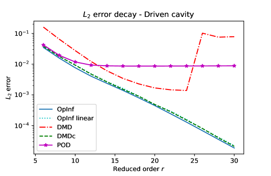
Figure 8: driven cavity: $L_{2}$ errors between the velocities obtained using the original and other reduced-order models, obtained using various method and orders.

7.2.3 Example 2: cylinder wake

Now, we report the numerical experiments conducted for the cylinder wake example. We have considered the semi-discretized in space FOM of order $n_{\mathbf{v}}=5812$. For this example, we again compute $513$ velocity snapshots in the interval $[0,2]$ equally spaced in time which are generated using the implicit-explicit Euler scheme. Note that $\mathbf{g}(t)\equiv\texttt{const}$ and, hence, the snapshot matrix $\mathbf{V}$ does not satisfy the algebraic constraints. However, as explained in Section 6, we can construct the divergence-free snapshot matrix

$$\mathbf{V}_{0}=\Pi\mathbf{V}=\begin{bmatrix}\mathbf{v}_{\top}(t_{0}),\mathbf{v}_{\top}(t_{1}),\dots,\mathbf{v}_{\top}(t_{N})\end{bmatrix}$$

by means of the Leray projection, see (36), where $\mathbf{v}_{\top}(t)$ is the divergence-free velocity and, hence, $\mathbf{A}_{12}^{\top}\mathbf{V}_{0}=0$ holds. The POD surrogate model will then be computed using the velocity free-snapshots as stated in Section 6. On the other hand, data-driven methods such as OpInf and DMD to infer reduced models do not require such a transformation, and the original velocity snapshots can directly be used to learn models. This is due to the fact that there is a hidden quadratic ODE for the velocity $\mathbf{v}(t)$. Next, two POD bases are computed using the snapshot matrix $\mathbf{V}$ and another for the divergence-free velocity $\mathbf{V}_{0}$. Figure 9 depicts the decay of the singular values of these snapshot matrices as well as the algebraic error committed by the divergence-free POD basis.

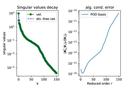
Figure 9: cylinder wake: We plot the decay of singular values (left) and show how the divergence-free POD basis satisfies the algebraic constraints (right).

Next, for $r_{\mathbf{v}}=30$, surrogate models are obtained using the different methodologies. To compare the qualities of these models, we perform time-domain simulations and compare them in Figure 10. We did not include the time-domain simulation for DMD, since the results could not follow the FOM behavior at all. Additionally, Figure 11 shows the pressure evolution obtained using OpInf. Moreover, we compute the relative time-domain $L_{2}$ errors for different orders between $8$ and $32$, and the results are depicted in Figure 8. As in the driven cavity example, OpInf, OpInf_lin and DMDc have a similar performance for the different reduced orders. Hence, for this example, the control term $\mathbf{\widehat{B}}$ is crucial for the identification of FOM.

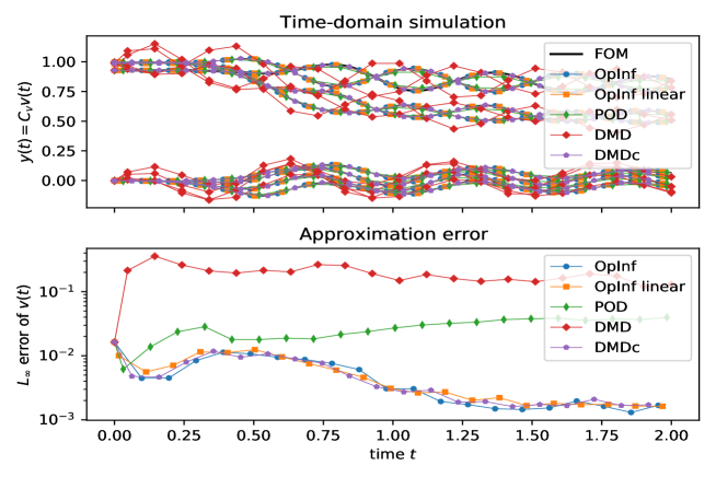
Figure 10: cylinder wake: A comparison of time-domain simulation of different models.

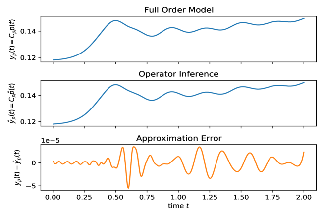
Figure 11: cylinder wake: Comparison of the pressure output for the original model and the inferred model using OpInf.

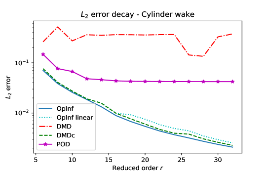
Figure 12: cylinder wake: $L_{2}$ errors between the velocities obtained using the original and other reduced-order models, obtained using various method and orders.

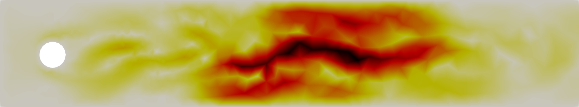
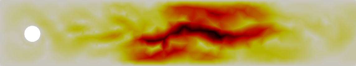
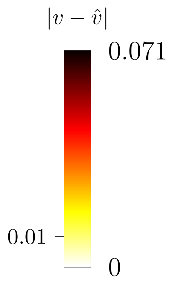
Figure 13: Errors $|\mathbf{v}(t)-\widehat{\mathbf{v}}(t)|$ for $r_{\mathbf{v}}=30$ at $t=2$ for the approximation via DMDc (top) and OpInf (bottom).

Code and Data Availability

The source code of the implementations, the raw data, and the scripts for computing the presented results are available via

doi:10.5281/zenodo.4086018

and GitHub under the MIT license.

Figure 14: Link to code and data.

8 Conclusions

In this paper, we have tailored the operator inference approach [35] to learn physics-informed low-order models for incompressible flows using data. We have shown that although the velocity and pressure are coupled in incompressible flow problems, one can identify a differential equation using only velocity snapshots that determine the velocity field’s evolution. Moreover, there exists an algebraic equation linking pressure and velocity. In Koopman’s philosophy, to learn dynamical systems, one can think of the velocity being the right observers to determine the evolution of pressure. Therefore, learning of differential and algebraic equations can be easily separated, and we can identify the underlying differential and algebraic equations using only data. In contrast to that, the projection-based approaches such as POD need to respect the differential-algebraic structure of the Navier-Stokes equations, in particular if there is inhomogeneity in the incompressibility constraint or if the basis vectors are not divergence-free. Furthermore, an affine-linear variant of DMD that is completely data-based too, showed very similar performance with operator inference. However, as illustrated in a small example, we expect to see a limit of DMD when the nonlinear term plays a significant role in defining the dynamics.

References

- [1] M. I. Ahmad, P. Benner, P. Goyal, and J. Heiland. Moment-matching based model reduction for Navier-Stokes type quadratic-bilinear descriptor systems. Z. Angew. Math. Mech., 97(10):1252–1267, 2017. doi:10.1002/zamm.201500262.
- [2] J. Annoni, P. M. O. Gebraad, and P. J. Seiler. Wind farm flow modeling using an input-output reduced-order model. In 2016 American Control Conference, ACC 2016, Boston, MA, USA, July 6-8, 2016, pages 506–512. IEEE, 2016. doi:10.1109/ACC.2016.7524964.
- [3] A. C. Antoulas, I. V. Gosea, and A. C. Ionita. Model reduction of bilinear systems in the Loewner framework. SIAM J. Sci. Comput., 38(5):B889–B916, 2016. doi:10.1137/15M1041432.
- [4] Z. Bai, E. Kaiser, J. L. Proctor, J. N. Kutz, and S. L. Brunton. Dynamic mode decomposition for compressive system identification. AIAA J., 58(2):561–574, 2020.
- [5] M. Baumann, P. Benner, and J. Heiland. Space-time Galerkin POD with application in optimal control of semi-linear parabolic partial differential equations. SIAM J. Sci. Comput., 40(3):A1611–A1641, 2018. doi:10.1137/17M1135281.
- [6] M. Behr, P. Benner, and J. Heiland. Example setups of Navier-Stokes equations with control and observation: Spatial discretization and representation via linear-quadratic matrix coefficients. e-print 1707.08711, arXiv, 2017.
- [7] P. Benner, P. Goyal, B. Kramer, B. Peherstorfer, and K. Willcox. Operator inference for non-intrusive model reduction of systems with non-polynomial nonlinear terms. Comp. Meth. Appl. Mech. Eng., 372:113433, 2020. doi:10.1016/j.cma.2020.113433.
- [8] P. Benner and J. Heiland. LQG-balanced truncation low-order controller for stabilization of laminar flows. In R. King, editor, Active Flow and Combustion Control 2014, volume 127 of Notes on Numerical Fluid Mechanics and Multidisciplinary Design, pages 365–379. Springer International Publishing, 2015. doi:10.1007/978-3-319-11967-0_22.
- [9] P. Benner, C. Himpe, and T. Mitchell. On reduced input-output dynamic mode decomposition. Adv. Comput. Math., 44(6):1821–1844, 2018. doi:10.1007/s10444-018-9592-x.
- [10] P. Benner, J. Saak, and M. M. Uddin. Balancing based model reduction for structured index-2 unstable descriptor systems with application to flow control. Numer. Algebra Control Optim., 6(1):1–20, 2016. doi:10.3934/naco.2016.6.1.
- [11] S. A. Billings and S. Y. Fakhouri. Identification of systems containing linear dynamic and static nonlinear elements. Automatica, 18(1):15–26, 1982.
- [12] T. Breiten, K. Kunisch, and L. Pfeiffer. Feedback stabilization of the two-dimensional Navier-Stokes equations by value function approximation. Appl. Math. Optim., 80(3):599–641, 2019. doi:10.1007/s00245-019-09586-x.
- [13] S. L. Brunton, J. L. Proctor, and J. N. Kutz. Discovering governing equations from data by sparse identification of nonlinear dynamical systems. Proc. Natl. Acad. Sci. USA, 113(15):3932–3937, 2016.
- [14] Z. Drmač and K. Veselic. New fast and accurate Jacobi SVD algorithm. I. SIAM J. Matrix Anal. Appl., 29(4):1322–1342, 2007. doi:10.1137/050639193.
- [15] A. Dumon, C. Allery, and A. Ammar. Proper general decomposition (PGD) for the resolution of Navier-Stokes equations. J. Comput. Phys., 230(4):1387–1407, 2011. doi:10.1016/j.jcp.2010.11.010.
- [16] F. Giri and E.-W. Bai. Block-oriented nonlinear system identification, volume 1. Springer, Berlin, Germany, 2010.
- [17] I. V. Gosea and A. C. Antoulas. Data-driven model order reduction of quadratic-bilinear systems. Numer. Lin. Alg. Appl., 25(6):e2200, 2018. doi:10.1002/nla.2200.
- [18] I. V. Gosea and I. Pontes Duff. Toward fitting structured nonlinear systems by means of dynamic mode decomposition. e-print 2003.06484, arXiv, 2020. URL: https://arxiv.org/abs/2003.06484.
- [19] C. Gräßle, M. Hinze, J. Lang, and S. Ullmann. POD model order reduction with space-adapted snapshots for incompressible flows. Adv. Comput. Math., 45(5):2401–2428, 2019. doi:10.1007/s10444-019-09716-7.
- [20] B. Gustavsen and A. Semlyen. Rational approximation of frequency domain responses by vector fitting. IEEE Trans. Power Del., 14(3):1052–1061, 1999.
- [21] P. C. Hansen. The L-curve and its use in the numerical treatment of inverse problems. In P. Johnston, editor, in Computational Inverse Problems in Electrocardiology, Advances in Computational Bioengineering, pages 119–142. WIT Press, 2000.
- [22] M. Heinkenschloss, D. C. Sorensen, and K. Sun. Balanced truncation model reduction for a class of descriptor systems with application to the Oseen equations. SIAM J. Sci. Comput., 30(2):1038–1063, 2008. doi:10.1137/070681910.
- [23] B. L. Ho and R. E. Kálmán. Effective construction of linear state-variable models from input/output functions. at-Automatisierungstechnik, 14(1-12):545–548, 1966.
- [24] X. Jin, S. Cai, H. Li, and G. E. Karniadakis. NSFnets (Navier-Stokes Flow nets): Physics-informed neural networks for the incompressible Navier-Stokes equations. e-print 2003.06496, arXiv, 2020.
- [25] J.-N. Juang and R. S. Pappa. An eigensystem realization algorithm for modal parameter identification and model reduction. J. Guidance, Control, and Dyn., 8(5):620–627, 1985.
- [26] J. N. Kutz, S. L. Brunton, B. W. Brunton, and J. L. Proctor. Dynamic Mode Decomposition: Data-Driven Modeling of Complex Systems. Society of Industrial and Applied Mathematics, Philadelphia, USA, 2016. doi:10.1137/1.9781611974508.
- [27] S. Le Clainche and J. M. Vega. Higher order dynamic mode decomposition. SIAM J. Appl. Dyn. Syst., 16(2):882–925, 2017.
- [28] J. R. R. A. Martins and J. T. Hwang. Review and unification of methods for computing derivatives of multidisciplinary computational models. AIAA J., 51(11):2582–2599, 2013. doi:10.2514/1.J052184.
- [29] A. J. Mayo and A. C. Antoulas. A framework for the solution of the generalized realization problem. Linear Algebra Appl., 425(2-3):634–662, 2007.
- [30] S. A. McQuarrie, C. Huang, and K. Willcox. Data-driven reduced-order models via regularized operator inference for a single-injector combustion process. e-print arXiv:2008.02862, 2020.
- [31] I. Mezić. Analysis of fluid flows via spectral properties of the Koopman operator. Annu. Rev. Fluid Mech., 45:357–378, 2013.
- [32] Y. Nakatsukasa, O. Sète, and L. N. Trefethen. The AAA algorithm for rational approximation. SIAM J. Sci. Comput., 40(3):A1494–A1522, 2018.
- [33] N. Nguyen, A. T. Patera, and J. Peraire. A best points interpolation method for efficient approximation of parametrized functions. Internat. J. Numer. Methods Engrg., 73(4):521–543, 2008.
- [34] B. Peherstorfer, S. Gugercin, and K. Willcox. Data-driven reduced model construction with time-domain Loewner models. SIAM J. Sci. Comput., 39(5):A2152–A2178, 2017.
- [35] B. Peherstorfer and K. Willcox. Data-driven operator inference for nonintrusive projection-based model reduction. Comput. Methods Appl. Mech. Eng., 306:196–215, 2016.
- [36] J. L. Proctor, S. L. Brunton, and J. N. Kutz. Dynamic mode decomposition with control. SIAM J. Appl. Dyn. Syst., 15(1):142–161, 2016.
- [37] J. L. Proctor, S. L. Brunton, and J. N. Kutz. Generalizing Koopman theory to allow for inputs and control. SIAM J. Appl. Dyn. Syst., 17(1):909–930, 2018. doi:10.1137/16M1062296.
- [38] E. Qian, B. Kramer, B. Peherstorfer, and K. Willcox. Lift & learn: Physics-informed machine learning for large-scale nonlinear dynamical systems. Physica D: Nonlinear Phenomena, 406:132401, 2020. doi:10.1016/j.physd.2020.132401.
- [39] M. Raissi. Deep hidden physics models: Deep learning of nonlinear partial differential equations. J. Machine Learning Research, 19(1):932–955, 2018.
- [40] M. Raissi, P. Perdikaris, and G. E. Karniadakis. Multistep neural networks for data-driven discovery of nonlinear dynamical systems. arXiv preprint arXiv:1801.01236, 2018.
- [41] M. Raissi, P. Perdikaris, and G. E. Karniadakis. Physics-informed neural networks: A deep learning framework for solving forward and inverse problems involving nonlinear partial differential equations. J. Comput. Phy., 378:686–707, 2019.
- [42] S. S. Ravindran. Reduced-order adaptive controllers for fluid flows using POD. J. Sci. Comput., 15(4):457–478, 2000. doi:10.1023/A:1011184714898.
- [43] P. J. Schmid. Dynamic mode decomposition of numerical and experimental data. J. Fluid Mech., 656:5–28, 2010. doi:10.1017/S0022112010001217.
- [44] M. Schoukens and K. Tiels. Identification of block-oriented nonlinear systems starting from linear approximations: A survey. Automatica, 85:272–292, 2017.
- [45] L. Sirovich. Turbulence and the dynamics of coherent structures. I. Coherent structures. Quart. Appl. Math., 45(3):561–571, 1987.
- [46] G. Stabile, S. Hijazi, A. Mola, S. Lorenzi, and G. Rozza. POD-Galerkin reduced order methods for CFD using finite volume discretisation: vortex shedding around a circular cylinder. Commun. Appl. Indust. Math., 8(1):210–236, 2017. URL: https://content.sciendo.com/view/journals/caim/8/1/article-p210.xml, doi:https://doi.org/10.1515/caim-2017-0011.
- [47] G. Stabile and G. Rozza. Finite volume POD-Galerkin stabilised reduced order methods for the parametrised incompressible Navier-Stokes equations. Computers & Fluids, 173:273 – 284, 2018. doi:https://doi.org/10.1016/j.compfluid.2018.01.035.
- [48] J. H. Tu, C. W. Rowley, D. M. Luchtenburg, S. L. Brunton, and J. N. Kutz. On dynamic mode decomposition: Theory and applications. J. Comput. Dyn., 1(2):391–421, 2014.
- [49] M. O. Williams, I. G. Kevrekidis, and C. W. Rowley. A data-driven approximation of the Koopman operator: Extending dynamic mode decomposition. J. Nonlinear Sci., 25(6):1307–1346, 2015. doi:10.1007/s00332-015-9258-5.
- [50] M. O. Williams, C. W. Rowley, and I. G. Kevrekidis. A kernel-based method for data-driven Koopman spectral analysis. J. Comput. Dyn., 2(2):247–265, 2015.
- [51] A. Wills, T. B. Schön, L. Ljung, and B. Ninness. Identification of Hammerstein-Wiener models. Automatica, 49(1):70–81, 2013.
- [52] S. Yıldız, P. Goyal, P. Benner, and B. Karasozen. Data-driven learning of reduced-order dynamics for a parametrized shallow water equation. e-print arXiv:2007.14079, 2020.