A correlation between the dark content of elliptical galaxies and their ellipticity.
Abstract
Observations indicate that the baryonic matter of galaxies is surrounded by vast dark matter halos, which nature remains unknown. This document details the analysis of the results published in Ref. [32] reporting an empirical correlation between the ellipticity of elliptical galaxies and their dark matter content. Large and homogeneous samples of elliptical galaxies for which their dark matter content is inferred were selected using different methods. Possible methodological biases in the dark mass extraction are alleviated by the multiple methods employed. Effects from galaxy peculiarities are minimized by a homogeneity requirement and further suppressed statistically. After forming homogeneous samples (rejection of galaxies with signs of interaction or dependence on their environment, of peculiar elliptical galaxies and of S0-type galaxies) a clear correlation emerges. Such a correlation is either spurious –in which case it signals an ubiquitous systematic bias in elliptical galaxy observations or their analysis– or genuine –in which case it implies in particular that at equal luminosity, flattened medium-size elliptical galaxies are on average five times heavier than rounder ones, and that the non-baryonic matter content of medium-size round galaxies is small. It would also provides a new testing ground for models of dark matter and galaxy formation.
1 Scope of this document
This document is an archival article that details the analysis performed in Ref. [32] to investigate the relation between the amount of dark matter in elliptical galaxies and their shape. A significant correlation was found and reported in [32]. Here, we provide the details of the analysis method, the data used and the systematic studies conducted to understand the nature of the correlation and the influences of specific factors such as the environment of the galaxies. We also provide a similar analysis as that performed in [32], but for the baryonic mass rather than the dark mass. No similar correlation is found.
2 Introduction
Dark matter is an essential ingredient of cosmology. It provides together with dark energy for a consistent description of many large-scale features of the universe [63]. However, at the galactic and semi-galactic scales, open questions remain [1, 80]. There, galaxies are depicted as constituted of a vast dark matter halo surrounding a smaller baryonic component. One method to advance our understanding at the galactic scale is to look for relationships between the dark matter content of a galaxy and its observed luminous matter. Useful empirical relations have been found, e.g. that of Tully-Fisher [101] for spiral galaxies which links the galactic rotation speed to the galaxy absolute luminosity. For elliptical galaxies, a prominent empirical correlation is the “Fundamental Plane" [37, 38] which combines the Kormendy [66] and the Faber-Jackson [41] relations and links the galactic effective radius , the surface brightness and the dispersion of stellar velocities . Intriguingly, none of these correlation directly involve dark matter. Equally puzzling is the observation that some elliptical galaxies harbor little dark matter [87]. We discuss here the correlation between the defining characteristic of elliptical galaxies –the ellipticity, on which e.g. their Hubble sequence is entirely founded– and their relative dark matter content, expressed as the total galactic mass (baryonic+dark) normalized to luminosity ( ratio).
The conventional Hubble classification groups galaxies into four broad morphological categories based on visual appearance: spiral, elliptical (with smooth featureless distribution), lenticular (with a bright central bulge and external disk but no spiral structure) and irregular (without well-defined structure). In this study, we focus on elliptical galaxies. Although those generally have tri-axial ellipsoidal structures and ellipticities depending on radii, to first approximation the geometric structure of elliptical galaxies can generally be simply modeled as oblate ellipsoids with constant ellipticities (). Those span a wide range, from (round galaxies) to (highly flattened ellipsoids). This essentially continuous variation of allows us to investigate how the general elliptical galaxy characteristics evolve with . A caveat, however, is that only the ellipticity projected on our observation plane (hereafter , the apparent ellipticity) is observed. The true ellipticity (henceforth ) can be inferred only by detailed modeling of the galaxy. Furthermore for elliptical galaxies are difficult to measure comparatively to disk galaxies [87]. These difficulties can be circumvented statistically: in a large and homogeneous samples of elliptical galaxies one can minimize the effects of galaxy peculiarities by a homogeneity requirement. The large number of galaxies further suppresses these effects statistically. Performing this analysis with extracted using different methods allows to minimize possible systematic bias associated with a particular method. Finally, the projection problem can also be addressed statistically: it is straightforward to model its overall effect on the studied correlation and correcting for it.
The actual shape of the dark halo remains an open question. A correlation between the amount of dark matter and the ellipticity of galaxies offers an opportunity to experimentally address this question as well as the fundamental questions of the interaction of baryonic and dark matter, and the present tensions between the standard model of galaxy formation and the data.
Throughout this document, the are expressed in solar unit and to characterize the shape of a galaxy (assumed to be oblate) we use its axis ratio where is the minor radius and the major radius. Finally, will stand for Distance Modulus, not dark matter.
3 Choice of data set and method
We used 42 separate publications that provide or related ratios for at least several elliptical galaxies. We also considered 24 other articles, but without using their results for reasons given in Appendix A. Overall, after selecting appropriate galaxies, we obtained 255 different galaxies for a total of 685 data points. Tables listing the galaxies used are given in appendices C to J. The last appendix presents our most detailed analysis, including a study of the interrelation between the various variables characterizing the galaxies to check whether the correlation with that was eventually identified could be a consequence of other correlations. We grouped the publications according to the methods used to extract (or related ratios such as with the part of the galactic mass from stars, or the dark matter fraction ). In the following sections we describe the methods, their advantages and caveats. In the subsections, we summarize our analysis for each data set and its specificities. We classified the results into reliability groups defined as:
-
•
Group 1: reliable results.
-
•
Group 2: somewhat reliable.
-
•
Group 3 somewhat less reliable.
-
•
Group 4: less reliable.
Authors whose work belong to groups 4 or 3 should not be offended: this grouping is pertinent solely in the context of the work relevance to our study, and not in any other sense: all the results are published in peer-reviewed journals (except for [16]) and thus should be reliable. This reliability criterion was used in Section 13 to weight the results when combining them. This procedure is coarse and might introduce some subjectivity but in practice, its effects turned out to be numerically small because lower reliability groups typically have lower statistics. After combining the results in Section 13, correcting them (Section 10.2) if necessary for the fact that the correlation was studied vs the projected axis ratio (apparent axis ratio ) rather than the intrinsic one (true axis ratio ), we present and discuss the global results in Section 13.
3.1 General selection criteria
For each publication, we chose of subset of the analyzed elliptical galaxies as homogeneous
as possible. This was done for two reasons:
1) it reduces the noise coming from effects peculiar to given galaxies
which would obscure a possible correlation with point-to-point uncorrelated variations;
2) it avoids biasing the studied correlation
with systematic effects from a class of galaxies, e.g. giant elliptical
galaxies (point-to-point correlated effect).
Our selection criteria are more strictly applied to sets of local galaxies and have to be
relaxed for sets of distant galaxies because these are not
characterized as accurately. (Typically, one can use only distant galaxies for strong
lensing analyses or those using the Fundamental Plane time-evolution,
see e.g. Ref. [61]).
The local and distant selection criteria are listed bellow, with galaxy characteristics obtained from either the NASA/IPAC Extragalactic Database (NED) [110] or from the publication that provided the . It is important to take notice that the selection criteria have been decided before carrying out the analysis. Thus, the analysis is “blind” with minimal subjective bias.
3.1.1 Local galaxies
When possible, only medium size elliptical galaxies were selected. Those tend to be “disky” and to have almost isotropic random velocities. We also required the galaxies to be undisturbed because galaxy interactions often compromise the applicability of the formulae used to extract the dark matter content (e.g. strong lensing equations, virial theorem, hydrostatic equilibrium equations). We reject galaxies that are, according to the NASA/IPAC Extragalactic Database (NED) [110] or the article in which is calculated:
-
•
Lenticular galaxies (S0-type);
-
•
Active Galactic Nucleus (AGN) galaxies because an AGN may signal a recent disturbance of the galaxy. Furthermore, AGNs emit at all wavelengths and can consequently bias our study by lowering the ratios;
-
•
LINERS galaxies (because they may be due to AGN), Seyfert (Sy) and BL Lacertae objects (BLLAC) active galaxies, for the same reasons as AGN;
-
•
Peculiar galaxies, or any galaxy listed in the Arp catalogue [111] of peculiar galaxies;
-
•
Giant elliptical galaxies (D), supergiant elliptical galaxies (cD), Brightest Cluster Galaxies (BrClG), EXG [112] and XE galaxies. These galaxies belong to different classes of elliptical galaxies, tend to be triaxial and moreover, the “boxy” giant galaxies are characterized by anisotropic random velocities. In addition, the determination of their amount of dark matter could be skewed by contribution from the cluster or group the galaxy belong to; Further reasons to reject large elliptical galaxies are provided in [17];
-
•
Compact elliptical galaxies (cE);
-
•
E? galaxies in the NED because the lack of definite morphology assignment may reflect poor measurements and may contaminate our galaxy set with non-elliptical galaxies;
-
•
Transition-type (E+) and galaxies formerly described as elliptical but now identified as spiral galaxies;
-
•
HII emission galaxies, because it may signal a recent disturbance. In any case, the presence of HII regions is unusual for elliptical galaxies, making those to fulfill the “peculiar galaxy” rejection criterion. HII emission might also bias the determination because newly born blue stars increase significantly the luminosity ;
-
•
VCXG galaxies [112] since they show signs of disturbed hydrostatic equilibrium.
-
•
NELG (narrow emission line galaxy) galaxies since it may signal a recently disturbed galaxy.
We keep LERG (low excitation radio galaxies) and WLRG (weak emission-line radio-galaxies) since we saw no obvious reason to exclude them.
3.1.2 Distant galaxies
Distant galaxies are usually not well enough characterized to apply the above criteria. Nevertheless, they are very useful to include in our study since typically only distant galaxies are available to apply the strong lensing method e.g. [2] or [59] or that of the Fundamental Plane time-evolution, e.g. [61] or [86]. The rejection criteria for distant galaxies are:
-
•
Massive galaxies, with typically . This criterion should minimize the amount of contamination of our sample by cD, D or BrClG galaxies. The choice for mass selection is based on the work of Ferreras et al. [46]: the authors noted that galaxies with behave differently that those with ;
-
•
Galaxies with relatively low velocity dispersions, km.s-1, if S0 and elliptical galaxies are not separated but considered altogether in the publication, or if the classification may not be reliable enough. This should suppress possible S0 contamination: S0 tend to have km.s-1. We verified that, within a sample of well identified local elliptical galaxies, rejecting the genuine elliptical galaxies with km.s-1 does introduce a bias of the vs correlation, see Section 4.6.2. Hence, this criterion is adequate to reject S0 without biasing our study.
In addition, if some of the characteristics listed in Section 3.1.1 are available (such as AGN or known interaction with another galaxy), then these galaxies are also rejected.
3.2 Uncertainties
Since all the data sets will be eventually combined in a single overall determination of vs. , the uncertainties for and must be estimated consistently lest galaxy samples with optimistic determinations of their uncertainties will be given an unwarranted preponderance. In addition, some publications do not provide any uncertainties and these then need to be assessed without the detailed knowledge of the analyses carried in the publication. To obtain a consistent determination of the uncertainties, we employ the unbiased estimate, i.e, we re-scaled the uncertainties111If the uncertainties are not provided in the publication, we assume to be proportional to , assume no uncertainty on , and then apply the unbiased estimate method. so that, when a fit of vs. is performed, its is set to unity. This supposes a gaussian dispersion of the data of a given galaxy set. For the fit, we choose it to be linear for simplicity and to minimize the number of fit parameters. If the true dependence of vs. is not linear, then the would increase which in turn would increase the final uncertainties when is set to unity. Hence, the linearity assumption is accounted for in the final uncertainty.
A caveat of forcing to unity when fitting vs apparent axis ratio comes from the fact that a large part of the data scatter is not due to the data gaussian dispersion. Rather, it is due to the random projection of the real 3D shape of the galaxy onto our 2D observation plan, see Section 10.2 and in particular Fig. 43 or 44. Still, we adopte the procedure of forcing because 1) it is the simplest method to estimate uncertainties when data are provided without uncertainties; 2) we can apply the same procedure to all data sets for consistency; and 3) it was a conservative procedure, as discussed above.
Finally, conscious that some assumptions underlie the fit procedure and the unbiased estimate method, we independently assessed the degree of correlation using the Pearson correlation coefficient.
3.3 Systematic studies
In sections 4 to 9, we summarize the analyses made on each galaxy set for obtain vs . When possible, the systematic effect associated with a particular galaxy characteristic was also studied. This was done when the set contained a large enough number of galaxies and the galaxy characteristic was provided. We list below these auxiliary studies.
-
•
Effect of galactic metallicity using the Lauer data [69] based on the virial theorem. (no effect) ;
-
•
Influence of the correlation between and central luminosity density, using the Lauer data [69] based on the virial theorem. (Large effect);
-
•
The effect of luminosity was also studied using the Auger et al. data [2] based on lensing. This also check the correlation with galaxy boxy/disky shape: more luminous galaxies tend to be boxy and less ones tend to be disky. No correlation between the and the luminosity/boxy-disky galaxy character was observed.
-
•
Effect rejecting bona-fide galaxies with low velocity dispersion, using the Prugniel & Simien data [84] based on the virial theorem. (No effect);
-
•
Effects of LINERS, using the Prugniel & Simien data [84] based on the virial theorem. (No effect);
- •
-
•
The effect of environment was studied using the Auger et al. [2], Barnabe et al. [5] and Cardone et al.(2009, 2011) [21, 22] data sets based on lensing. Galaxies residing in clusters tend to show a smaller vs axis ratio correlation (smaller slope) with more jitter (larger relative uncertainty). The lensing data set from Cardone et al.(2009) [21] shows, however, the opposite trend.
-
•
The effect of choosing a particular initial mass function (IMF) to interpret the data can be checked with the Auger et al. [2] and Barnabe et al. [5] data sets based on lensing, and the Deason et al. [30] data employing PNe and GC. See also the Cappellari et al. [17] data based on using light profile measurements and stellar orbit modeling.
4 Data sets using virial theorem
Galactic mass-to-light ratio can be extracted using the virial theorem. Its simple form (scalar virial theorem) gives where is the stellar velocity dispersion, a proportionality coefficient, a given radius (e.g. the effective radius or the core radius) and is the surface brightness. The value of is in principle the same for galaxies of an homogeneous sample. The formula assumes spherical symmetry and a virialized system. The ellipticity of the galaxy can be accounted for using the tensor virial theorem, see [3] and references within. The data discussed in this section were obtained using ellipticity corrected virial formulae. When the published data did not account for ellipticity, we used the Bacon et al. [3] ellipticity corrections formula (simplified formula using central dispersion only and ). This correction, derived analytically, is important. It was independently verified by the results of van der Marel [104], see Section 5.6. In addition, without this correction, the averaged would be too small compared to an expected value around 8 . We remark that the modification to the (spherical) Newton Shell Theorem to include ellipticity yields a similar figure, see Section 7.
Caveats for this method of extracting are:
-
•
Anisotropy effects are generally not accounted for;
-
•
Only for the galaxy inner part are obtained. This one tends to be rounder and dominated by baryonic matter, thereby biasing and diluting the effect we study;
- •
Another potential caveat of this method is that unphysical correlations between and can be induced by anisotropic star motions. However, this should not be an issue because, as assessed in Ref. [3], the effect is small. Furthermore anisotropies have little effects on the slopes of Figs. 1a and 1b of [3] whilst affecting primarily the absolute values. Because we are investigating a dependence of on , the absolute scale of is of secondary importance. Therefore, possible effects of the anisotropies are not critical. Furthermore, the absolute values of will be normalized to the expected =8 when all the data sets are combined, see Section 13. In addition, bright galaxies –which tend to display these anisotropies– are discarded from our samples by our selection criteria. Our assessment that anisotropies should be of small concern was a posteriori justified by checking that the results from [3] –which used a large set of galaxies and the virial method– displayed no significant vs brightness correlation, see the correlation study in appendix L.
4.1 Bacon et al. (1985)
Bacon et al. [3] extracted ( in the B-band) for 197 early-type galaxies. We analyzed these data thoroughly using additional selection criteria222We required in addition to the selection criteria described in 3.1.1 that the galaxy characteristics listed in the 1985 Ref. [3] are compatible with the up-to-date (as of 2008, when the analysis was performed) characteristics provided in the NED [110]. and studying possible correlations between various galaxy characteristics that could have biased our study. The full analysis is presented in appendix L. Depending on data availability, ellipticity corrections formulae of various accuracies were used.
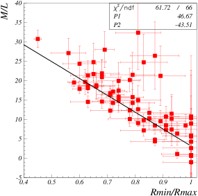
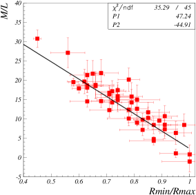
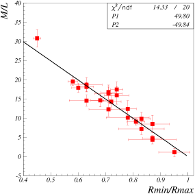
After applying the selection criteria, we were left with of 64 elliptical galaxies in our main sample (Sample 1). Better ellipticity corrections are available for 11 galaxies (Sample 2). The results of fits to these data using the Bacon et al. values for and distance moduli are shown in Figs. 1, 2 and 3 and are:
for Sample 1 (ellipticity corrections from isotropic method).
for Sample 2 (ellipticity corrections from isotropic method, where is the quadratic sum of the galaxy velocity and its central velocity dispersion , see [3]).
for Sample 2 (ellipticity corrections from anisotropic method).
The uncertainties on were taken as the difference between the Bacon et al. and NED values. The uncertainties are from Bacon et al., rescaled so that (unbiased estimate).
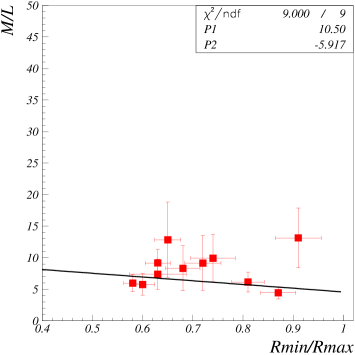
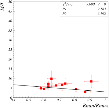
There are several advantages to this data set:
The virial formula used to obtain the published is
corrected for galactic ellipticity;
The large data set (197 galaxies) allowed
strict criteria to be used to remove unsuitable or suspicious galaxies;
Three methods were used to obtain ;
Triaxial galaxies were excluded
from the original data set, as they are less suited for the virial
method.
The analysis is dated (1985) but we have used only data consistent with the more recent NED numbers, so we do not consider this to be an important caveat. We assigned the results to group 2 reliability for Samples 1 and 2 with ellipticity corrections from the isotropic method, and reliability group 1 for Sample 2 with ellipticity correction from the anisotropic method.
4.2 Bender et al. (1989)
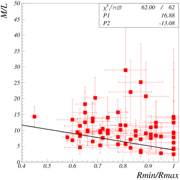
Bender et al. [6] analysis assumed spherical symmetry. There was 109 galaxies in the original sample. After selection, we retained 35 galaxies. vs apparent axis ratio is shown in Fig. 4. The fit result for the 35 selected galaxies (using NED values for with a uncertainty) is:
.
The uncertainty was assigned to be proportional to with the overall scale factor adjusted so that .
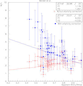
Specific caveats of this analysis are: the analysis is dated; There were frequent large discrepancies between the values used in the original analysis and the NED values (e.g. redshift, ellipticity or luminosity values); No uncertainty was provided.
We remark that the values without ellipticity corrections appear to be too low: in average, . Using the more modern value for the Hubble constant km/s/Mpc rather than 50 km/s/Mpc as used by the authors, we obtained . This is well below the expected (minimal) value of for an elliptical galaxy without dark matter contribution, and with dark matter contribution. This proves the necessity of the ellipticity corrections. We assigned the results to group 3 reliability.
4.3 Kelson et al. (2000)
Kelson et al. [61] determined the internal kinematics, length scale and surface brightness of 53 galaxies from cluster CL1358+62, 11 of them elliptical galaxies. The data were used to form . Applying an absolute magnitude selection to minimize the contamination from boxy galaxies would have left only one available galaxy. Relaxing the selection to left 5 galaxies to study. We applied the ellipticity corrections from Bacon et al. [3]. The vs apparent axis ratio is shown in Fig. 5. Uncertainties were slightly scaled to force .

The best linear fit is:
.
The specific caveats of this analysis are that the galaxies are not as well characterized (morphology, spectra) as local ones, and they belong to a dense cluster. Thus, they may not be in virial equilibrium, and we cannot apply the usual strict criteria that select galaxies likely to be in virial equilibrium. Consequently, we assigned these data to group 4 reliability.
For completeness, the fit before ellipticity ellipticity corrections yields .
4.4 Lauer (1985)
The Lauer data set [69] contains 42 galaxies. was extracted from the stellar velocity dispersion in the galaxy core, assuming a spherical star distribution. Thus, the were determined for radii . The ratios were given without uncertainty estimates. The uncertainty we assigned did not follow our standard procedure: we assigned a constant uncertainty of rather than because of the low outlier at , see Fig. 6. With the standard procedure, the outlier would have had a very small uncertainty and would have driven the fit. The value is chosen so that . Lauer classified galaxies in 3 classes, depending on the quality of the core resolution. Class 1 is for well resolved cores, class 2 for partially resolved cores and class 3 for unresolved cores. In addition to for the core, Lauer provided a secondary analysis that determined more globally using effective radius rather than the core radius, which extends his analysis beyond the galaxy core. However, because his main analysis concerns galaxy cores, we will consider only rather than . We applied our usual selection criteria with, as in Section 4.1, the added requirement that the galaxy characteristics listed in Lauer’s 1985 publication are compatible with the one in NED [110], with the exception of the axis ratio because it was not provided in [69]. We used the NED values for the axis ratios. The sample was reduced to 10 galaxies after selection. If we had restricted the sample to galaxies with resolved (class 1) or partially resolved (class 2) cores, only two galaxies would have remained (one in class 1: NGC 720 and one class 2: NGC 7619). Hence we did not apply this additional requirement and used galaxies from the 3 classes indiscriminately.
The dependence with axis ratio is shown in Fig 6. The fit results gives:
.
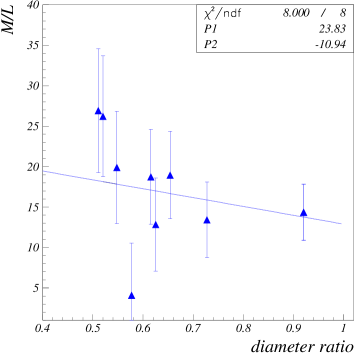
The data set has several specific caveats: it is dated and no ellipticity correction was originally done. The ratios were computed for the galaxy cores and given without uncertainty estimates. The uncertainty was determined following a particular procedure rather than our standard one due to an outlier having a value close to 0. Because of the above caveats, we assigned the results to group 4 reliability.
For information we note that:
-
•
Before applying ellipticity corrections the fit was: .
-
•
Results using the more recent NED distances [110] are: .
-
•
Results for the global mass to light ratio are: . Using the more recent NED distances: . The opposite correlation sign appears to be spurious and due to correlations between the luminosity density and on the one hand and and on the other. This is discussed next.
Correlations
Correlation with metallicity
Lauer noticed a correlation between galaxy metallicity and . Indeed we found and . However, we found no clear correlation between and . Consequently, the relation between and should not induce the correlation oberved between and .
Correlation with central luminosity density
Lauer also signaled a correlation between the luminosity density and . We found and . Notice the opposite correlations between central and effective densities. There is no clear correlation between and , whilst a correlation exists between and : . Thus, the correlation between and may be biased by, or even due to, the () and () correlations. This can explain the opposite (positive) sign of the (, ) correlation compared to the (negative sign) (, ) correlation: subtracting the correlation from , we get , consistent with the negative slope in and the expectation that below should not vary strongly. We will not use the results in the global analysis of Section 13.
4.5 Leier (2009)
4.6 Prugniel & Simien (1996)
4.6.1 Main study
Prugniel & Simien [84] compiled kinematics and photometric data for 371 early-type galaxies. They remarked that this set might be biased toward flat galaxies since those are preferably chosen for major axis kinematic measurements. This should be of no consequence in our context. We selected adequate elliptical galaxies following the usual morphology and emission criteria. We did not use the galaxies from the PCG catalog, although some seem to be good elliptical galaxies, since they all have low velocity dispersions. The set obtained contains 102 galaxies.
We formed from the virial theorem and corrected it for ellipticity using the virial tensor correction formula from Bacon et al. [3]. The galaxy type and characteristics, including axis ratio, were obtained from NED. The uncertainties were assumed to be proportional to and set so that . vs apparent axis ratio is shown in Fig. 7.
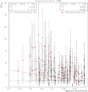
The best linear fit is:
.
The advantage of this analysis is that the data are numerous and relatively recent compared to the other extractions of that used the virial theorem. The only specific caveat of this analysis is that no uncertainties are provided. We assigned these results to group 2 reliability.
For information, the result before applying the ellipticity corrections is: .
4.6.2 Systematic studies
Effect of a velocity dispersion selection
The large sample of well identified elliptical galaxies provided the opportunity to check the effect of removing from the sample good elliptical galaxies with low velocity dispersion km.s-1). Such selection is applied in the analyses of distant galaxies that have less reliable type identification, in order to minimize possible S0 contamination. However, this selection may at the same time also remove genuine elliptical galaxies. Thus, it is important to check if a low velocity dispersion selection produces a bias. Once the km.s-1 criterion was applied, only 44 galaxies out of 112 remained. The mean value of increased significantly because . However, normalizing the fit result to the same average value as in the main study yielded a correlation similar to that of the main study:
,
This indicates that no bias arises from the the km.s-1 criterion. This test is statistically significant because more than 50% of the 112 galaxies has been removed. (We performed the same study on data without ellipticity corrections and reached the same conclusion).
Effects of LINERs
We added 17 LINER elliptical galaxies to the main sample. The best fit from this larger sample including LINERs agrees well with the main result given in previous section. However, this is not statistically significant because the sample size increased only by 13% (from 112 to 127 galaxies). We also checked the results of the linear fit using only LINERs and found it compatible with the main data (again with large statistical uncertainty). However, we notice that:
-
•
The LINER distribution may be biased toward apparently rounder galaxies: 94% of LINER have , for only 76% of our non-LINER sample. If true, this could bias the magnitude of the and correlation in the case of the LINER if that correlation is not linear (e.g. a weaker correlation at high values would lower more the average vs slope in the case of LINERs).
-
•
The shape of the vs distribution is similar for LINER and non-LINER. The are both flat before ellipticity corrections and thus similar after applying identical ellipticity corrections.
4.7 Retturaet al. (2006)
Rettura et al. [86] studied the relation between galaxy stellar masses and dynamical masses for a sample of 37 elliptical, 5 lenticular and 6 bulge-dominated spiral galaxies. was obtained by matching the spectral energy distribution to composite stellar population model templates obtained from stellar population models in which a Kroupa Initial Mass Function -IMF- [68] was assumed. Several models were used but the results are not strongly model-dependent. includes masses from stars and stars remnants (white dwarves, Black Holes,…) masses. was computed assuming that galaxies are spheroidal non rotation-supported systems in virial equilibrium: . From the 37 elliptical galaxies, we formed a sample excluding known AGN, two interacting giant galaxies belonging to the CL1252 cluster, O-II emission galaxies, E+A galaxies, and large X-ray emission galaxies. Furthermore, because the morphology of the galaxies is not as well known as for local galaxies, we excluded galaxies with velocity dispersion km.s-1 to minimize possible S0 contamination (this selection could a priori bias our investigation because of the relation . However, our study in Section 4.6 indicated no such bias). Our final sample contains 16 galaxies. The axis ratios are obtained from [102], [40] or [55]. We assumed a uncertainty on them. We applied the ellipticity corrections from Bacon et al. [3]. The vs apparent axis ratio is shown in Fig. 8.

The best linear fit is:
.
Advantages of this analysis are that the stellar component was calculated differently from the other analyses and the data are relatively recent. A caveat is the additional model dependency (stellar population model, IMF choice) of the method. In addition, the galaxies are not as well characterized (morphology, spectra) as local ones. We assigned these data to group 3 reliability.
For completeness, the fit before ellipticity corrections yields ).
4.8 van der Welet al. (2006)
In Ref. [102], van der Wel et al. used a similar galaxy set as Rettura et al. [86]. The vs apparent axis ratio is shown in Fig. 9. We apply the ellipticity corrections from Bacon et al. [3]. There are 13 galaxies in our sample.

The best linear fit is:
.
As for Rettura et al. [86], we assign these data to group 3 reliability.
For completeness, the fit before ellipticity correction yields )
5 Data using light profile measurements and stellar orbit modeling
This approach relies on modeling the stellar dynamics of galaxies using photometry data at different radii (light profile). Potentials for stellar and dark components are assumed and the light of the stars moving in the total potential is simulated. Parameters of the potentials are adjusted until the models match the data. We applied on the data sets the usual homogeneity selection criteria. However, when models did not rely on virial or isothermal equilibrium, we have relaxed the standard selection and include LINERS, AGN and Seyfert galaxies. An advantage of this method is that the true ellipticity of the galaxy can be inferred and accounted for in the determinations of . A caveat is that the results are necessary model-dependent.
5.1 Cappellari et al. SAURON IV data set (2006)
Cappellari et al. [17] used stellar photometry data to provide at for 25 nearby bright elliptical galaxies. Careful extraction of is argued, leading the authors to estimate a 6% error on and 10% on stellar mass to light ratios, . The true ellipticity was input in the calculations. It was obtained by modeling the photometry data. The authors chose to work with the velocity dispersion at , , rather than the central velocity dispersion because is less sensitive to the aperture used for the observation device, and to details of orbitals. Out of an initial sample of 48 galaxies the authors selected 25 galaxies, requesting them to have accurate distance determination, a Hubble Space Telescope WFPC2 photometry and no strong evidence of a bar. After our selection we obtained a set of 6 galaxies. The authors provided two estimates of . One is based on a 2-integral Jeans model (numerically accurate but less general) and one on a 3-integral Schwarzschild model [92] (numerically noisier but more general). The authors cautioned that large elliptical galaxies (more massive and slow rotators, redder and more metal rich) tend to be tri-axial, which may alter the determination. The fits to the vs ellipticity are shown in Fig. 10. The best fits, slightly corrected for the stellar dependence with the intrinsic axis ratio are:
and
.
The fit result for the stellar population is .
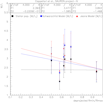
The analysis is based on a robust extraction, with true ellipticity and projection effect accounted for. We assigned the results to group 1 reliability.
5.2 Cappellari et al. ATLAS project (2013)
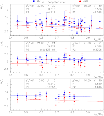
The data used here come from two publications from Cappellari et al. [19, 20]. The authors analyzed a set of 32 elliptical galaxies using either the Salpeter IMF or the JAM model for modeling the light distribution. The authors also provide a quality factor for their extracted and ellipticities, classifying each galaxy model from 0 (lower quality) to 3 (better quality). Thus, in addition to the full galaxy sample, we also considered two subsamples, the largest containing 23 galaxies with models of quality 1 to 3, and a smaller sample of 12 galaxies with models of quality 2 or 3. (The quality 3 model provides a sample of only 4 galaxies, a too small sample to be of use). The fits to the vs axis ratio are shown for the full sample and subsamples in Fig. 11. The best fits for these samples are:
Quality 0-3, Salpeter IMF:
Quality 0-3, JAM model:
—
Quality 1-3, Salpeter IMF:
Quality 1-3, JAM model:
—
Quality 2-3, Salpeter IMF:
Quality 2-3, JAM model:
The used in the analysis are robust and the true ellipticities are assessed consistently. Thus, we assigned the results to group 1 reliability.
As the four (sub)samples are not independent, we can use only one of them when combining all the data reported in this article to obtain an overall correlation. We used the results from the full sample (32 galaxies).
5.3 Kronawitter et al. (2000)
Kronawitter et al. [67] used non-parametric spherical models to map the gravitational fields of 21 round elliptical galaxies. From the maps, in the inner (central ) and outer (outermost kinematic data point) parts of the galaxies were calculated. The technique used here did not rely on isothermal or virial equilibrium. We thus rejected only the cD, S0, peculiar, cE, SA0 and Arp galaxies present in the initial sample, keeping in particular LINERS, AGN and Seyfert galaxies. We remark that after standard selection, only three elliptical galaxies would have remained. This relaxed selection provided a sample of 10 galaxies. To estimate the model uncertainty, we took the difference between low and high values provided in [67]. In addition, we added an uncertainty proportional to to account for possible experimental uncertainties that would be common to the low and high estimates. The uncertainties were adjusted so that for the best fits. The authors estimated the effects of non-sphericity on their data and we corrected their based on their numbers. Fig. 12 shows vs apparent axis ratio. The best fits to the data are:
.
.
The ratio was originally determined at the outermost kinematic data point with varying between 0.45 and 2.95, a domain where the dependence of with radius becomes important. To obtain the at the same radius value (, the average value for ), we interpolated or extrapolated the authors results.

The caveat of this data set is that the galaxies are chosen preferentially round. In the case of , the smaller uncertainties on two galaxies (NGC3640 and NGC3379) drives the fit results. An advantage of the analysis is the correction for (apparent) ellipticity. We assigned the results to group 1 reliability.
5.4 Magorrian et al. (1998)
Magorrian et al. [73] modeled 32 galaxies to obtain and central black hole mass (the main goal of [73]). The models assumed that galaxies are axisymmetric with an arbitrary inclination (not provided in the article), have a constant , and have a central black hole. The models did not include anisotropies. The black hole, stellar and dark matter gravity fields were obtained respectively from a fit to Hubble Space Telescope (HST) photometry data, a given and assuming a given constant . Jeans equations were used to obtain velocity and velocity dispersion profiles that were compared with ground based data. The ground based and HST data do no extend further than and are typically a few tenths of . After our standard selection, 7 galaxies remained. We used axis ratios from NED. The uncertainty was symmetrize and rescaled so that . vs apparent axis ratio is shown in Fig. 13.
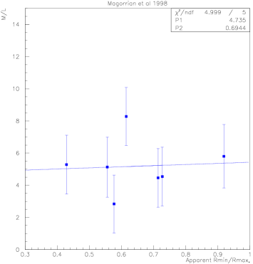
The best fit is:
.
A caveat is that the models do not include anisotropies. is assumed to be constant, which is now known to be incorrect in general but is probably valid in the radial range addressed in this study. Advantages of the analysis are the corrections for ellipticity and inclination. We assigned the results to group 1 reliability.
5.5 Thomas et al. (2007, 2011) and Wegner et al. (2012)
Thomas et al. [97] studied 19 galaxies from the Coma cluster. Dark and luminous masses were obtained within using a dynamical model employing Schwarzschild orbit superposition techniques [92]. Galaxies were assumed to be axisymmetric and in dynamical equilibrium. The flattening of the galaxies was included in the model, although only 3 possible values for the galaxy inclinations were considered: 90∘ (assumes ), minimum inclination (assumes the galaxy is a E7) and intermediate inclination (assumes galaxy is a E5). A Log or a Navarro-Frenk-White (NFW) [81] profile was used for dark matter distribution and it was assumed that the baryonic mass profile is the same as the light emission profile (mass follows light assumption). Using these mass profiles, the potential was calculated and all possible orbits were determined. The light profiles obtained were compared to the data and the best fit determined the best model. The authors cautioned that, although this procedure should determine the most likely of the 3 possible inclinations, the selection procedure may be biased toward the 90∘ case. The uncertainty on was calculated by accounting for all possible inclinations. We rescaled it so that our fit is 1. The authors computed the lens characteristics of their galaxies, although there is no known lensing observation from them, in order to compare their results to the SLACS strong lensing results, see sections 9.1 and 9.2. From this they provided, in the -band, a dark matter fraction () within the Einstein radius .
The same group that reported in [97] used the same methods and tools to analyze 8 early-type galaxies from the Abell 262 cluster (Wegner et al. [108] ). We can thus add these data to the ones of [97]. Differences between the two works include:
-
•
The Abell 262 cluster is less densely populated than the Coma cluster, so these galaxies are less liable to interaction with environment;
- •
- •
Four galaxies from [97] and three galaxies from [108] passed our selection criteria. The mass over light ratios and within are shown in Fig. 14. is obtained from the relation .
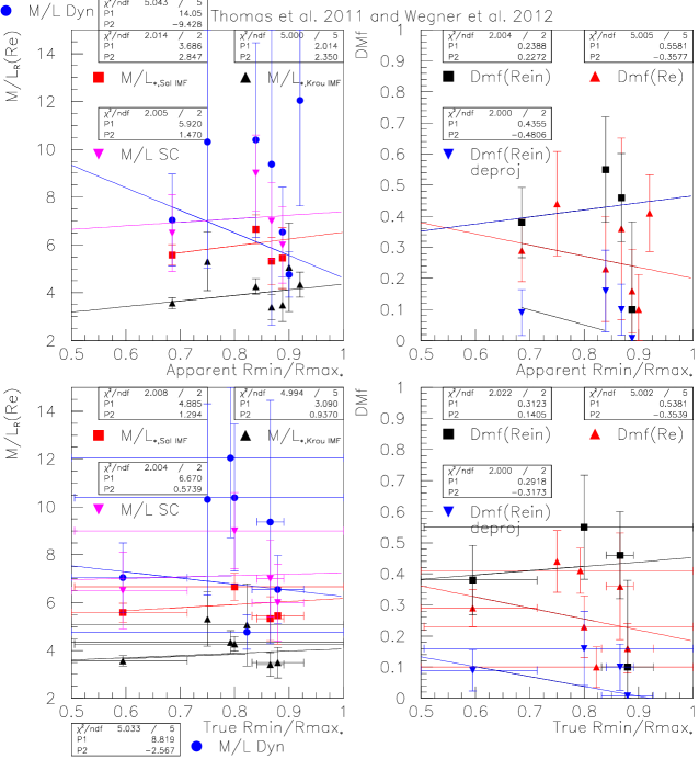
The best fits are:
,
for the apparent axis ratio and:
,
for the true axis ratio.
The fit parameters obtained with apparent and true axis ratios are compatible, as expected since the uncertainties cover all 3 assumed inclinations.
The advantage of this analysis is that the effect of ellipticity was fully accounted for, although necessarily in a model dependent way and with only 3 possible values for the galaxy inclination. The caveat of this study is that the galaxies belong to a cluster. They thus may be subject to their environment. The results were assigned to group 1 reliability.
For information, we show other quantities in Fig. 14 : the stellar computed using a Kroupa or Salpeter IMF (available only from [97]); : this quantity assumes that the total mass follows light, i.e, is independent of the galaxy radius. This assumption has been ruled out for by many recent studies, including the one of Thomas et al.; Projected and deprojected : these quantities are available only from [97]. They depend on the choice of linear relation between and , which is rather arbitrary. The procedure is adequate in the context of [97] but somewhat arbitrary for our purpose.
The best fits for these quantities are:
,
,
,
,
for the apparent axis ratios and
,
,
. (We will use this result for our global analysis with a reliability factor 2)
,
for the true axis ratios.
5.6 van der Marel (1991)
In [104] van der Marel constructed axisymmetric dynamical models for 37 local early-type galaxies selected for their high quality photometry. The models include anisotropy and rotation but kept constant with radius. was obtained by fitting the major and minor axis kinematics, which is more accurate than core fitting using the virial theorem. However, the author checked his work by also computing using the virial tensor formula of Bacon et al. [3] which includes ellipticity but assumes to be constant with radius. The two results, and correlate well but the virial results are in average smaller. The good correlation confirms Baconet al. [3] formula, which we used throughout Section 4 to correct results that did not account for the galaxy ellipticity. To form , the mass density was obtained by deprojecting the luminosity profile and assuming . From that density, the gravitational potential was calculated by solving the Poisson equation. Finally, the Jeans equations, which assume hydrostatic equilibrium, were solved. was calculated for two inclination angles: and but the difference is small: is larger by about 10% for axis ratios of about 0.7 and, as expected, disappears for axis ratios near 1. The used here are the average between the and results. The author computed the axis ratios using his models. We used the average of his result with the NED axis ratio, the difference being taken as uncertainty. The ratios vs apparent axis ratios are shown in Fig. 15 for the 9 galaxies that passed selection. In addition to the standard selection criteria, we further rejected S0 candidates (NGC636, 3557, 4494 and IC0179) and S (NGC1370) galaxies, although they are listed as elliptical galaxies in NED.
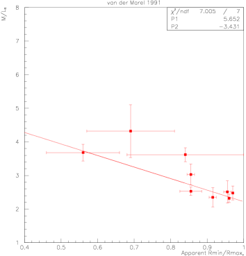
The best fit is:
).
We rescaled the uncertainties so that . The advantage of the analysis is that care has been taken in accounting and studying the effects of apparent ellipticities, inclination angles, anisotropies and rotations. The caveats are that the analysis is dated, but this is balanced by the author’s galaxy selection based on the high quality of their photometry. The models assumed hydrostatic equilibrium, which we enforced by strict selection that removes about two thirds of the original galaxy sample. Finally a constant is assumed. This is known to be incorrect at large radii, as the author and many other studies found, but this is reasonable at radius up to . We assigned the results to group 1 reliability.
5.7 van der Marel and van Dokkum (2007a)
In Ref. [105], van der Marel and van Dokkum studied 25 early-type galaxies using stellar rotation and velocity dispersion data. The galaxies belong to 3 clusters at redshift (except for one field galaxy. But we will ignore it as it is classified as a E/S0). The data were interpreted with oblate axisymmetric 2-integral dynamical models based on Jeans’ equations of hydrostatic equilibrium. was assumed to be constant with radius. This assumption has been ruled out by many recent studies (e.g. [67, 97, 104, 16, 74, 78, 79, 9]), although it appears reasonable in the radius range considered here (). Using the inferred probability distribution of true axis ratio for elliptical galaxies, the authors computed for each galaxy a most-likely true axis ratio. This one was calculated by taking the average over all possible values of the true axis ratio for a galaxy () weighted by the true axis ratio probability distribution. The resulting “true” axis ratio may not be the actual one but is a reasonable guess that follows the expected gaussian distribution of true axis ratios. The galaxies in [105] were identified only by visual inspection. To address the possibility of S0 contaminating the galaxy set, we estimated the probability to be a S0 using the expected characteristics of S0 ( tends to be lower, high rotational support and strong ellipticity dependence with radius. We did not consider the additional fact that ellipticities of S0 are large to not bias our study). Based upon this criteria, of the 25 galaxies 7 were unlikely to be S0 (none of those are listed as S0 in [105]), 12 were possibly S0 (4 listed as S0 or E/S0 in [105]) and 6 were likely to be S0 (1 of those is a known S0/Sb). Assuming that about half of the 12 possible S0 are indeed S0, the 25 early-type sample contained about 13 E and 12 S0, agreeing with the known repartition of the local E and S0 galaxies. Removing the 5 galaxies listed in [105] as visually identified as S0, E/S0 or S0/Sb, we obtained Sample 3 of 19 galaxies. Removing from it 5 galaxies that are likely to be S0 based on our criteria, we obtained Sample 2 (15 galaxies). Finally considering only the galaxies unlikely to be S0, we obtained Sample 1 (7 galaxies). The ratios vs apparent and true axis ratios are shown in Fig. 16. We can see that the S0 rejection criteria removed the low points, possibly biasing our study. To address this, we did not use this criteria for the determination of the slopes but only to estimate the uncertainty due to possible S0 contamination.
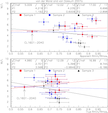
The best fits are:
for Sample 1,
for Sample 1,
for Sample 2,
Sample 2,
for Sample 3,
for Sample 3.
All in all using the samples 1 and 2 to estimate the S0 contamination to the main sample (sample 3), we obtain:
,
.
The uncertainties from [105] were rescaled so that . Advantages of this study are that ellipticity was mostly accounted for in the calculations, and a true ellipticity was tentatively given. Caveats of this analysis are the lack of good galaxy identification (S0 contamination) and of features revealing possible disturbance, whereas the extraction assumes hydrostatic equilibrium. Thus, we could not implement our standard selection of undisturbed galaxies. An uncertainty for the S0 contamination was assessed using tight selection. Other caveats are the redshift may cause systematic differences between the sample and local galaxies, and that was assumed to be constant. Finally, the positive fit slopes are driven by a single galaxy of large ellipticity and small uncertainty: CL1601-2040. As can be seen in Fig. 16, all slopes would be negative without CL1601-2040. However, we had no reason to exclude it from the study. The unbias estimate method partly accounted for this outlier. Since the S0 and outlier issues are reflected in the final uncertainty, the results are still assigned to group 2 reliability rather than a lower reliability group.
5.8 van der Marel and van Dokkum (2007b)
In order to compare the results of the previous section with results from local galaxies, van der Marel and van Dokkum compiled from the literature a homogenized for 60 early-type galaxies [106]. The were corrected using a consistent distance determination and, if needed to be, re-expressed in the B-band. The redshift of the galaxies forming the set is . All the literature sources compiled in [106] were also used in the our present study: van der Marel: Section 5.6, Magorrian et al.: Section 5.4, Gebhardt et al.: Section A, Kronawitter et al.: Section 5.3 and Cappellari et al.: Section 5.1. However, it is still interesting to consider the compilation of [106] because results have been homogenized. Applying our standard selection to the initial 60 galaxies, we obtained a sample of 17 galaxies. The sources contribute with similar statistics (van der Marel: 8 galaxies, Magorrian et al.: 5 galaxies, Kronawitter et al.: 4 galaxies, Gebhardt et al.: 6 galaxies, Cappellari et al.: 6 galaxies). Hence, our final sample is a representative average rather than being strongly bias toward a particular work. The ratio vs apparent axis ratio is shown in Fig. 17.
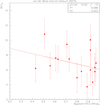
The best fit gives:
.
The advantages and caveats of these data are already discussed in the sections 5.6 (group 1 reliability), 5.4 (group 1 reliability), A (data unused, due to low statistics and correlations), 5.3 (group 1 reliability) and 5.1 (group 1 reliability). Most of these data were already used for our analysis, although they have been homogenized and averaged when a particular galaxy was available from several of the literature sources. The results are assigned to group 1 reliability but partly weighted out when we considere the global results incorporating all vs axis ratio, see Section 13.
6 Data sets using Planetary Nebulae and Globular Clusters
Planetary Nebulae (PNe) and Globular Clusters (GC) provide well resolved tracers extending to large radii. They offer the possibility to examine individual stars (PNe) or compact stelar assemblies (GC) to robustly assess the gravitational potential over a large radial range. Caveats of this method in our context is that the ellipticity determined from photometry might not match the ellipticity at large radii, and that the tracers at large radii may be influenced by the cluster or group hosting the galaxy. A general concern with GC is that they may be decoupled from the evolution their host galaxy: they are good tracers of the overall gravity field but may have a different rotational structure and whilst PNe tend to follow the light distribution, GC tend to be more extended. However, this is unimportant in the context of our study. Furthermore, since GC tend to belong to heavier galaxies which typically do not fulfill the selection criteria, the role of GC in our study is minimal.
All the literature sources used below assumed spherical symmetry. To account for ellipticity, we noted that the ellipticity corrections to the virial method (Section 4) and the X-ray method (Section 7) are close, as can be seen by comparing our Fig. 22 to the figures 1a and 1b of Bacon et al. [3]. We assumed the same correction to the extracted from PNe and GC data.
6.1 Capaccioli, Napolitano and Arnaboldi (1992)
Capaccioli, Napolitano and Arnaboldi [16] provided a compilation from the literature on . The mass to light ratio for 14 galaxies was obtained from PNe tracers (no GC) at two different radii (inner and outer ), so that the gradient could be calculated. The radii at which the were given differ from galaxy to galaxy so we interpolated linearly between the inner and outer to obtain a value at for all the galaxies. Following the authors, we used uncertainties of 10% and 30% for the inner and outer respectively, and propagated them to . None of the galaxies in [16] passed our selection criteria. Relaxing the selection to include all galaxies except the disrupted ones, galaxies showing possible interactions and clear non-elliptical galaxies, we obtained a set of 5 galaxies: NGC 1379 (maybe a spiral), 1700 (EXG), 3379 (LINER, VCXG), 4406 (SO(3)/E3) and 4697 (LLAGN). The fit to the vs axis ratio is shown in Fig. 18. The best fit is:
.
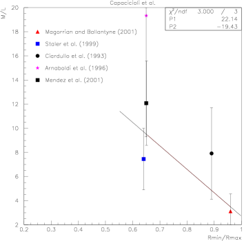
Caveats are that the data were obtained from difference sources (which may result in author-to-author bias) and include galaxies of unsure type, cD, LINERS and LLAGN. We assigned the results to group 3 reliability.
For information, the best fit before ellipticity corrections is:
.
6.2 Deason et al. (2012)
Deason et al. [30] employed PNe and GC as kinematic tracers to provide and integrated up to a radius of 5. The was extracted model dependently using either a Chabrier/Kroupa [25]/[68] or a Salpeter [89] Initial Mass Function (IMF). The authors studied 15 galaxies using a spherically symmetric model. The model allowed to form line of sight velocity distributions that were matched to the measured ones using a maximum likelihood method. It was assumed that the tracers’ orbit are dominated by random motion rather than systematic motion. Furthermore, any possible galaxy rotation was ignored and simple power-law profiles for tracer density and potential were assumed. Velocity anisotropies were accounted for. The potentials and anisotropy parameters were determined by the best fit to the measurements of the tracer line of sight velocity distribution. From this, the mass was extracted. The usual galaxy selection yielded a first sample (Sample 1) of 4 good elliptical galaxies (NGC 821, 1344, 3377 and 4564). For this analysis, we can relax the selection to include LINERS, Sy, VCXG and LLAGN galaxies. We obtained then Sample 2 with 3 additional galaxies NGC 3379, 4374 and 4697. vs is shown on Fig. 19. The fits yield:
for sample 1 and
for sample 2.
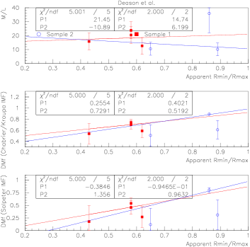
We assigned the result to group 1 reliability and used Sample 2 when combining all the publication together into one global result in Section 13.
For information, the best fits before ellipticity corrections
are:
for sample 1:
,
for the Chabrier/Kroupa IMF and
for the Salpeter IMF.
For Sample 2:
,
for the Chabrier/Kroupa IMF and
for the Salpeter IMF.
6.3 Magorrian and Ballantyne (2001)
Magorrian and Ballantyne [74] used PNe data to compute for 18 round early-type galaxies. The following method was employed: the velocity dispersion was calculated assuming a form and using Jeans equations and the luminosity density. This one was obtained from the measured surface brightness deprojected assuming a spherically symmetric galaxy. The obtained was fit to measured stellar or PNe velocity dispersions. The best fit determined the free parameters of the assumed form.
After we applied our standard selection, 6 elliptical galaxies remained. We used values of integrated up to . The vs stellar axis ratios are shown in Fig. 20.
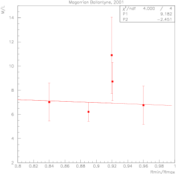
The best fit yields:
.
Advantages of this analysis are that the authors provided a detailed study of the effect of anisotropy and spherical asymmetry assumptions. They concluded that anisotropies have a small effect on whilst the spherical symmetry is a critical assumption with large effects on . The difficulty is that the effects of anisotropies or flattening are not distinguishable on the observed velocity dispersion data whilst, as just said, the magnitude of their influence on the value is different. According to [74] their spherically symmetric model underestimates . We assigned the result to reliability group 1.
For information, the best fit before ellipticity corrections is:
.
6.4 Romanowsky et al. (2003)
Romanowsky et al. [87] used kinematics of PNe to extract the rotation curves of three elliptical galaxies, each of them possessing about a hundred of observable PNe. The possible effect of anisotropies was studied with a spherical Jeans model in which an anisotropy parameter spans its full possible range. From the model, were obtained. Furthermore, a different method was used with NGC3379 to investigate the effect of velocity anisotropy variation with radius. The true axis ratios of the galaxies investigated in [87] had been inferred in [17] , [48] and [95]. The vs axis ratios are shown in Fig. 21.
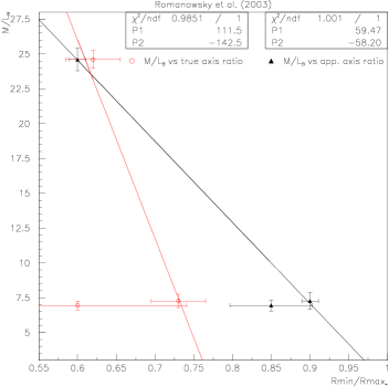
The best fits are:
,
,
where we rescaled the uncertainties on both and
so that the fit . An advantage of this work
is the detailed study of the effect of anisotropies using two different
techniques. We assigned the results to group 1 reliability.
For information, the best fits before ellipticity corrections are:
,
.
7 Data sets using X-ray
The extraction of a galaxy mass from X-ray emitting interstellar medium (ISM) data assumes that 1) the hot gas is in hydrostatic equilibrium under the galaxy gravitational potential: , and 2) that the gas follows the perfect gas law: . Here, is the ISM gas pressure, its density, its temperature, the gas molecule average mass ( MeV) and is the Boltzmann constant. can be extracted by combining the two previous equations: .
In the context of our study, this method has caveats. X-ray emission occurs mostly in giant galaxies, usually the one dominating its group or cluster (cD galaxies). Hot gas is highly collisional and can be heated by inner processes (electromagnetic emissions) or outer influences (galaxy interacting with its environment) and hence may be off equilibrium. In fact, results may correlate with the galaxy environment, as found in Das et al. [29].
All publications used here assumed spherical symmetry. We can partly account for ellipticity effects by replacing Newton’s shell theorem used to derive by a relation accounting for the ellipticity. In Fig. 22, we show the gravitational force in function of the axis ratio of an oblate spheroid of constant density, normalized to the force one would obtain if it were computed from Newton’s shell theorem. We set the mass of the spheroid to be independent of the axis ratio. Thus the density increases with ellipticity. This is relevant for a galaxy of known mass (luminosity) and unknown density333To obtain similar results at constant density (relevant to galaxies of known density but unknown luminosity), one should take the results of Fig. 22 and multiply them by the axis ratio , because an oblate spheroid volume is (4/3). However, this case is irrelevant to us. . Although this simple correction is only accounting for part of the ellipticity effects, we have used the median case in Fig. 22 to correct the X-ray data.
7.1 Fukazawa et al. (2006)
X-ray data from Chandra X-ray Observatory satellite were used by Fukazawa et al. [49] to extract the temperature profiles of 53 elliptical galaxies. Each luminosity profile was obtained assuming a de Vaucouleur law [39]. Values for were provided at . After standard selection, our final sample contains 7 adequate elliptical galaxies. vs axis ratio (from NED) is shown in Fig. 23. No uncertainties were provided in [49], so we assumed them to be proportional to their corresponding , and adjusted them so that the best fit has The best fit to the data yields:
.
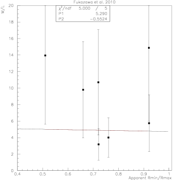
The caveats of these results are as follow. Our correction for ellipticity is basic (see Section 7). There is no correction for the asymmetry of the gas distribution (due e.g. to AGN jets), although this particular caveat is alleviated by our selection requirement. No uncertainties were provided. Because of the simplicity of the ellipticity corrections, the possible gas asymmetry effects and the absence of provided uncertainties, we assigned the results to group 2 reliability.
For information, the fit before ellipticity correction is:
.
7.2 Nagino and Matsushita (2009)
Nagino and Matsushita [78] used X-ray data from the XMM-Newton and Chandra satellites to extract integrated up to 3 different radii (0.5, 3 and 6) for 22 early-type galaxies. To obtain , the temperature and density profiles were deprojected assuming the ISM to be spherically symmetric. Likewise, the luminosity was deprojected to obtain the stellar mass profile assuming spherical symmetry and a de Vaucouleur profile [39]. After standard selection, 4 galaxies remain. was extracted both in the B-band and K-band. We assumed the uncertainties to be proportional to the corresponding values, with . However, only two points are available for 6 so is undefined. In that case, we used the average of the uncertainties from 0.5 and 3. The axis ratios are from NED.
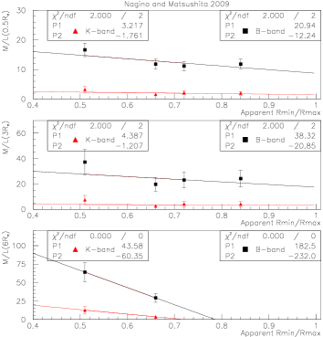
The best fits (shown in Fig. 24) are:
,
,
,
.
The lines going through the 2 data points at 6 are:
,
.
As for the results from Section 7.1, we assigned these
results to reliability group 2.
For information, the fit results before ellipticity
correction are:
,
,
,
.
The lines going through the 2 data points at 6 are:
,
.
8 Data sets using warm or cold gas disk dynamics
Cold hydrogen gas (HI) can be found in some elliptical galaxies. It extends to large distances (). is determined using ionized gas disks embedded in the galaxies as kinematical tracers. Ionized warm gas can also be used but warm gas disks are less extended and thus can be determined only in the inner regions. The are obtained the same way as for spiral galaxies, i.e, using a model with visible and dark component potentials to match the disk rotation curve. Thus virial or hydrostatic equilibrium is not assumed and our usual selection criteria can be relaxed. A caveat for our study with this method of determination is that extended HI rings are located mostly in S0 galaxies. In most cases elliptical galaxies with HI disks are gas rich, and thus are unusual among elliptical galaxies.
8.1 Bertola et al. (1991 and 1993)
Bertola et al. [9] provided for inner regions () of 5 elliptical and 2 galaxies using ionized gas disks. They also determined values for the outer regions of 4 elliptical galaxies using HI disks (). They had already used the same technique to obtain the inner ) for NGC5077, see [8], which we added to the sample. All galaxies are LINERS and/or Sy type. Their true ellipticities were obtained by fitting data with a tri-axial model for four of the elliptical galaxies and one of the lenticular galaxies. The best fit for the 4 elliptical galaxies is (see Fig. 25):
for
the 4 elliptical galaxies,
where and are the radii of the triaxial shape model for the elliptical galaxy.
Uncertainties were not given. We assumed that ,
with the proportionality constant such as in the
fit. We assigned a uncertainty on the intrinsic “axis
ratio” . We did not include the galaxy in
the fit reported above. Including it changes little
the results, except that the correlation is more marked. Using the
5 elliptical galaxies for which are provided and determining
the correlation with the apparent axis ratio ,
we found:
.
This illustrates the importance of the galaxy projection effect.
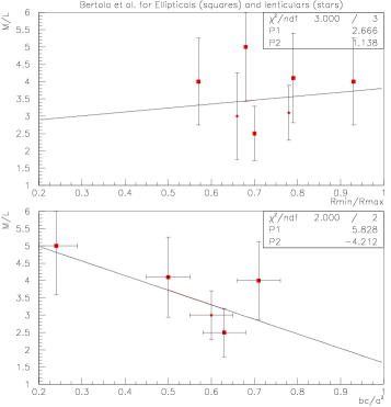
The data analysis accounted for the true shapes of the galaxies, so that there was no need of projection correction. The analysis used special galaxies (presence of a gas disks, Sy2, LINERS) and no uncertainty was given. On the other hand, the method is robust (similar to determination for spiral galaxies). We assigned the result to group 1 reliability.
8.2 Pizzella et al. (1997)
Pizzella et al. [83] used the velocity field measurements on ionized warm gas disks embedded in 4 elliptical galaxies to obtain their gravitational potentials. For each galaxy, an intrinsic triaxial galactic shape was obtained, which was argued by the authors to not be strongly model-dependent. The galactic mass integrated up to the maximum available radius was obtained from the velocity field. The modeling worked well for 3 galaxies but not as well for NGC7097 (which has a counter-rotating core). All galaxies are LINERS and two (NGC2974 and 5077) are Sy galaxies. We kept NGC7097 because its results are published nonetheless and its intrinsic ellipticity (, where and are the intrinsic axis ratios of the triaxial galaxy) is close to the one given by Bertola et al. [9]. was obtained from the potential and the light density profile. vs apparent and intrinsic axis ratios are shown in Fig. 26.

The best fits are:
,
.
The uncertainties on were scaled so that ,
and a uncertainty was assumed for the intrinsic axis ratio.
The bias for using apparent rather than intrinsic axis ratios is clear
(the effect of using the true shape rather than the projected one
to get is already accounted for). We assigned the
results to reliability group 1.
9 Data sets using strong lensing
Strong lensing has become a standard technique to extract . Its advantage is that the determination of , the total mass within the Einstein radius , is in principle model independent. Obtaining at other radii necessitates assuming a mass profile. Since strong lensing galaxies are distant, a light profile must be assumed too. Nevertheless, the method is the least model dependent way to obtain a galactic total mass. Virial or hydrostatic equilibria are not assumed, so our tight selection can be relaxed, keeping in mind that evidence of starburst or H-II emission can bias by affecting the luminosity. Selection enforcing a homogeneous galaxy sample (i.e, discarding cD, S0, cE galaxies…) is still necessary. Although equilibrium is not required, internal or external shears due to interaction with nearby neighbors can bias the determination of the mass. They are usually corrected for by the authors, although such correction is not unambiguous. Lensing galaxies are often found in clusters or groups. Our systematic study of the effects of environment shows that the galaxies in groups or clusters display more dispersion around their vs correlation, see Sections 9.1, 9.2 and 9.4 (we found the opposite in Section 9.3 but it may be a statistical fluctuation). This is expected if unaccounted galaxy-galaxy interactions cause a data jitter. In addition, the correlation slope seems larger for isolated galaxies.
A general caveat of this technique is that the probability of observing lensing from a galaxy is low so the known ones are distant. Consequently, their detailed characteristics are not known. In addition, distant galaxies may be at different evolution stages compared to the local ones. Furthermore, lensing equations bias samples toward heavier elliptical galaxies on the one hand, and higher ellipticity on the other hand. whilst the galaxies are at large redshifts , we chose to not correct for a possible - correlation because it is unclear whether it comes from structure evolution (as investigated e.g. in [60]), or from structure and sample bias (lensing sample biased toward flatter galaxies, with flatness correlating with ).
9.1 Auger et al. (2010)
Auger et al. [2] modeled the light and mass of 73 early-type galaxies based on photometric and strong lensing data from the Sloan Lens ACS (SLACS) survey [12]. The galaxies are located at redshifts. The data are interpreted with a de Vaucouleur profile [39] for photometry and a SIE (Singular Isothermal Ellipsoid) for the mass profile. The interpretation includes the effects of (apparent) ellipticity. From this, was estimated at . S0 galaxies were identified so we did not apply the standard km.s-1 criterion for this analysis (and all other analyses using SLACS data).
9.1.1 Analysis on full sample of Elliptical galaxies
We kept 34 elliptical galaxies, rejecting S0 galaxies (we relied on the identification from [1]) and minimizing the contamination of giant galaxies by requesting (the masses were taken from [53]). Mass axis ratios ,444 is the axis ratio of the modeled mass system. apparent axis ratios and luminosities are from [12]. If none were provided for a given galaxy, it was rejected. In addition, we rejected the galaxies signaled by the authors as significant fit outliers in the size-- correlation space. The vs axis is shown in Fig. 27. The best fits give, for the results derived with a SIE model using a Chabrier IMF [25]:
and, for results derived with a Salpeter IMF [89]:
.
For the mass ratio, we have:
(Chabrier),
(Salpeter).
Using apparent axis ratio rather than mass, we obtain for the Chabrier IMF:
and, for the Salpeter IMF:
,
Chabrier),
(Salpeter).
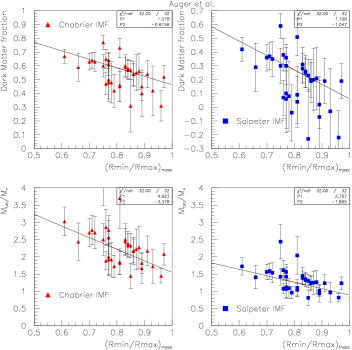
The published uncertainties were rescaled slightly so that . We assigned the results using a Chabrier IMF to reliability group 1.
9.1.2 Luminosity and environment study
Subsamples of galaxies allowed us to study the effect of luminosity (correlating with the boxy/disky galactic shape) and environment on these results:
-
1.
Subsample 1 contains elliptical galaxies not found in clusters according to Treu et al. [99] (17 elliptical galaxies);
-
2.
Subsample 2 contains elliptical galaxies found in clusters (17 elliptical galaxies);
-
3.
Subsample 3 contains elliptical galaxies with magnitude . This selects less massive disky galaxies (25 elliptical galaxies);
-
4.
Subsample 4 contains elliptical galaxies with magnitude and no generic selection on the total mass. This selects more massive boxy galaxies (17 elliptical galaxies);
-
5.
Subsample 5 contains elliptical galaxies with magnitude and not found in clusters (13 elliptical galaxies).
Subsample 1 results
The best fit to the data obtained using a Chabrier IMF and mass axis ratio is:
and, for the Salpeter IMF and mass axis ratio:
.
Using apparent axis ratio, we obtain for the Chabrier IMF:
and, for the Salpeter IMF:
.
Subsample 2 results
The best fit to the data obtained using a Chabrier IMF and mass axis ratio is:
and, for the Salpeter IMF and mass axis ratio:
.
Using apparent axis ratio, we obtain for the Chabrier IMF:
and, for the Salpeter IMF:
.
Subsample 3 results
The best fit to the data obtained with a Chabrier IMF and mass axis ratio is:
and, for the Salpeter IMF and mass axis ratio:
.
Using apparent axis ratio, we obtain for the Chabrier IMF:
and, for the Salpeter IMF:
.
Subsample 4 results
The best fit to the data obtained using a Chabrier IMF and mass axis ratio is:
and, for the Salpeter IMF and mass axis ratio:
.
Using apparent axis ratio, we obtain for the Chabrier IMF:
and, for the Salpeter IMF:
.
Subsample 5 results
The best fit to the data derived with Chabrier IMF and mass axis ratio is:
and, for results derived with Salpeter IMF and mass axis ratio:
.
Using apparent axis ratio, we obtain for the Chabrier IMF:
and, for the Salpeter IMF:
.
9.1.3 Conclusion
The subsample results are generally compatible with the full sample ones. There is no clear difference between samples of luminous/boxy and of fainter/disky galaxies. Selecting field galaxies increased the slope whilst the ones in groups/cluster appeared to have a smaller slope. The correlation for field galaxies is also clearer (smaller relative uncertainty for the slope)
The caveats of the analysis are that apparent axis ratios were used. However, from the results of Barnabe et al. [5], considering intrinsic axis ratios rather than apparent ones has a small effect: the change in slope is compatible with 0: for the Chabrier results and for the Salpeter IMF. The results and the mass axis ratios are model dependent. The IMF dependency can be estimated by comparing the Salpeter and Chabrier IMF results.
9.2 Barnabe et al. (2011)
Barnabe et al. [5] modeled the dark matter and stellar contents within about 0.5 for 16 E and S0 galaxies from the SLACS survey. In addition, they used spectroscopic observations from other sources than SLACS to further constrain their models. The stellar content was obtained with a Stellar Population Synthesis model using a Chabrier or a Salpeter IMF. Independently, they obtained a lower limit on by using a “maximum bulge hypothesis”. The models provide intrinsic mass axis ratios and luminous axis ratios. We selected 10 elliptical galaxies, the rest being S0 galaxies or E for which (masses from [53]). Among the 10 elliptical galaxies, 2 are fast rotators and 8 are slow rotators, 4 belong to clusters and 6 are more isolated. We formed using and . The best fits yield for the correlation with intrinsic luminous axis ratio (see Fig. 28):
for the data computed with a Chabrier IMF,
for the data computed with a Salpeter IMF.
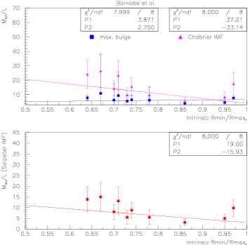
By fitting samples containing only isolated galaxies or galaxies belonging to clusters we check the effects of the environment on these results. The best fits yield for the galaxies not found in clusters:
for the data obtained with a Chabrier IMF,
with a Salpeter IMF,
and for the galaxies found in clusters:
for the data computed with a Chabrier IMF,
with a Salpeter IMF.
The isolated galaxies have a clearer, and possibly stronger, correlation as seen already in Section 9.1.
Finally, we checked the effect of the viewing angle projection on our analysis by repeating the analysis done on sample 1 but using the apparent light axis ratios rather than the intrinsic one:
for the data computed with a Chabrier IMF,
with a Salpeter IMF.
The projection effect is small and the fit values of the intrinsic and apparent cases are largely compatible. When the intrinsic axis ratio is used rather than the apparent one, the vs axis ratio slope decreases by about for the Chabrier result and by about for the Salpeter result. (The uncertainties determination assumes that the Chabrier and Salpeter data are uncorrelated, which is not true. Hence, the 59% and 70% uncertainties are overestimated.)
Advantages of this analysis are that it was done in term of real axis ratio and it used additional spectroscopic data. We assigned the results to group 1 reliability.
9.3 Cardone et al. (2009)
Cardone et al. [21] examined 21 early-type galaxies from the SLACS survey. Among them, 18 are elliptical galaxies (identification from [1]). The strong-lensing/photometry method was used to extract the up to the effective and Einstein radii, with a flexible ansatz that interpolated between several types of halo models. The preferred halo was selected by minimization. This reduces the model dependence of the determination compared to other strong-lensing/photometry results. Spherical symmetry was assumed, the ellipticity of the galaxies being accounted for only in the deprojection procedure to obtain luminosity profiles. The stellar was obtained from a Stellar Population Model using a Chabrier IMF. We formed from and . The apparent and mass axis ratios were taken from [12]. We compared the luminosities reported by the authors with those in [12] and rejected galaxies disagreeing by more than , and galaxies for which luminosities were not given in [12]. We also rejected 3 giant galaxies (, masses from [53]). All in all, we kept 13 galaxies (Main Sample). We split the Main Sample in two subsamples containing field galaxies (subsample 1, with 9 elliptical galaxies) and galaxies found in clusters (subsample 2, with 4 elliptical galaxies) [99]. The fits to or vs , shown in Fig 29, yield, for the quantities obtained at (uncertainties are from the 95% CL values of [21] scaled so that ):
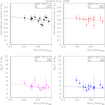
,
,
,
.
For the isolated galaxies (subsample 1), the best fits are:
,
,
,
.
For the galaxies found in clusters, the best fits are:
,
,
,
.
The trend is that, contrarily to the results in sections 9.1, 9.2 and 9.4, isolated galaxies have a weaker correlation than clustered ones. The low statistics may be the cause of this disagreement with the other studies.
Results obtained at the Einstein radius yield similar slopes ( and results are correlated). However, they should be less model dependent555 The and have still some model dependence because of the assumed luminosity and star mass profiles. than the results at . In average for our sample, . The best fits are:
,
,
,
.
For the isolated galaxies:
,
,
,
.
For the galaxies found in clusters, the best fits are:
,
,
,
.
An advantage of this analysis is the lesser model dependence claimed by the authors. A caveat is that the model assumes spherical symmetry. We assigned the results to group 1 reliability.
9.4 Cardone et al. (2011)
Cardone et al. [22] studied 59 early-type galaxies from the SLACS survey using a Secondary Infall Model which describes the collapse and virialization of a spherical halo. This theoretically sound model was for the first time employed to describe light and dark matter profiles. This allowed us, by comparing to other dark matter extractions, to investigate their model dependence. The study provided the total masses within . The was extracted using the stellar results from Auger et al. (with Salpeter IMF) [2]. We formed the using the luminosities given in [22]. Comparing them with the luminosities from [12], we found a 10% shift between the two results. We retained galaxies for which, apart for this 10% shift, luminosities from [22] and [12] agree within 15%. We also rejected 3 E/So galaxies, galaxies for which axis ratios were not available from [12] and giant galaxies (, masses from [53]). All in all, we obtained a sample of 36 galaxies. Using either mass or apparent axis ratios, the best fits are (see Fig 30):
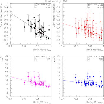
,
,
,
.
We checked the influence of environment by analyzing 2 subsamples in which galaxies that are isolated (20 galaxies) or belong to clusters (16 galaxies), according to [99]. For the isolated galaxies, the best fits are:
,
,
,
.
For the galaxies found in clusters, the best fits are:
,
,
,
.
Isolated galaxies display a stronger and clearer correlation than clustered ones, as already seen in sections 9.1 and 9.2.
This analysis is useful because it employed an original and physically founded model. Its caveats are its assumed spherical symmetry and usage of the old Salpeter IMF. We assigned the results to group 2 reliability.
9.5 Faure et al. (2011)
Faure et al. [44] examined 20 strong-lensing candidates from the COSMOS survey [109] and provided within effective and Einstein Radii for 12 of them. The lens candidates were tentatively identified as elliptical and galaxies. The galaxies are distant (redshift ). Standard strong-lensing and photometry methods to extract were used, with a Synthesis Model to infer the stellar mass and a SIE model for the total mass. The authors assumed that mass follows light: a Sersic profile [93] was used for both the mass and light distributions. Consequently, mass axis ratio and apparent axis ratios are equal. Effect of the environment was accounted for in the model. We formed from the authors’ and . Out of the 12 galaxies, we rejected two for which, according to [44], the model does not fit well the data (0047-5023 and 0050+4901) and one (5914-1219) for which the mass suggests that it is a giant. Furthermore, we rejected a galaxy (5921+0638) for which the ellipticity from [44] disagrees with [43] because of less reliable modeling. In addition, its low mass and low velocity dispersion suggest that it is a S0. Finally, we rejected a galaxy (0038+4133) with an unphysical and for which the low mass and velocity dispersion suggests again that it is a S0. The final sample contains 7 galaxies. The fits to or vs yield,666 We recall that it is assumed that . see Fig. 31:

,
.
To compare with other works providing we can use because for elliptical galaxies, typically. The specific caveats of this analysis are the “mass follows light” assumption (i.e, constant with ), which is believed to be invalid for , and that the model assumed spherical symmetry. We assigned the results to group 1 reliability.
9.6 Ferreras, Saha and Williams (2005)
Ferreras, Saha and Williams [46] compared the Einstein masses of 18 strong-lensing early-type galaxies to their visible masses obtained from photometry. The stellar model used had its parameters varied over a large volume of the parameter space, which should make the estimates robust [46]. is given in the V-band and depends on the choice of IMF. The authors determined with a Chabrier IMF but also provided it with a Salpeter IMF to assess the uncertainty attached to the choice of IMF. The masses given are contained within , which is a few : for our 4-galaxies sample 1.6, with in average . To select our sample, we rejected a galaxy known to be a spiral or S0 galaxy (B2237). To further suppress possible S0 contamination, we selected galaxies with km.s-1 (the are from [103], we slightly relaxed the usual km.s-1 otherwise only 2 galaxies would remain in the final sample). This rejected J0951, B0952, B1009, J1017, J1411, B1422 and B2149. We excluded galaxies with (B1104 and J1417). We rejected B0818 since it may be interacting with its environment and had no axis ratio available from literature. We rejected B1030 and B1608 because of interaction with environment. Finally B1115 was excluded as a peculiar galaxy. There are only 4 galaxies remaining after this selection (B0047, B0142, J0414 and B1520). We plot vs axis ratio in Fig. 32. The uncertainty is assigned so that =1. The best fits to the data yield:
for the Chabrier IMF,
for the Salpeter IMF.
The results were assigned to group 1 reliability.

9.7 Ferreras, Saha and Burles (2008)
Ferreras, Saha and Burles [47] fit photometric and strong lensing data from the SLACS survey [12] to extract for 9 E and S0 galaxies. The fit functions are based on models (de Vaucouleur profile for photometry and a SIE model for the mass profile). We kept 4 galaxies, rejecting 2 S0 galaxies (identifications from [1]), one galaxy for which and 2 galaxies for which the integrated was determined at significantly larger radius (1.66 and 2.01). The other were determined at . Ellipticities from [47] differ from the mass and apparent ellipticities from the SLACS survey article [12]. We assign an uncertainty on equals to the difference between the [12] and [47] values. The redshift correction to is small: there is at most a redshift difference of among the galaxies of the sample. From Keeton et al. [60], this implies a modification of of 5%, therefore we neglected it. The dependence with apparent and mass are shown in Fig. 33. The best fit results are:
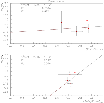
and
.
We assigned the results to group 1 reliability.
9.8 Grillo et al. (2009)
Grillo et al. [53] studied the stellar and dark matter content of 57 early-type galaxies from the SLACS survey. A Stellar Composite Model was used to obtain the stellar mass using two different sets of metallicity template and three different IMF (Salpeter [89], Kroupa [68], Chabrier [25]). The best choice was selected by the best fit to the galactic spectral energy density measurements. The total magnitude for each galaxy was obtained using a spherically symmetric de Vaucouleur profile. The total mass within was calculated via a SIE model, although the authors noted that with their choice of normalization, the mass should not depend on the ellipticity. After our standard SLACS selection, we retained 40 galaxies. The values of axis ratios used are from [12]. All uncertainties were symmetrized and scaled so that for our fits, . The fits, shown in Fig. 34, yield:
for the luminous model using a Salpeter IMF and a Maraston solar metallicity template (SMT) [75]. The corresponding is:
.
for a Salpeter IMF and a Bruzual & Charlot SMT [14]. The corresponding is:
.
for a Kroupa IMF and a Maraston SMT [75]. The corresponding is:
.
for a Chabrier IMF and a Bruzual & Charlot SMT. The corresponding is:
.
The analysis assumes spherical symmetry but the authors argued this to be of minimal importance. We assigned the results to group 1 reliability.
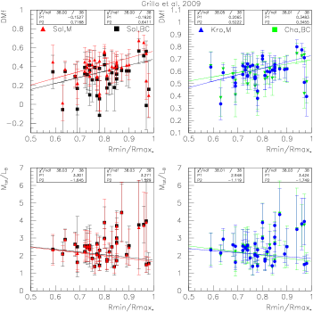
9.9 Jackson et al. (1998)
Jackson et al. [58] studied 12 lensing systems in the context of a “dark galaxy” search. within were inferred using a Singular Isothermal Sphere model for the mass distribution. We kept 4 galaxies out of the original 14 (2 lensing systems are double-lenses). We rejected B2114+022 G1 as a E+A galaxy that has in addition unreliable due to dust [26]. B1608+656, B1600+434, B1933+507 and B0218+357 are spiral galaxies. B2045+265 may be a Sa. Galaxies B1030+074 and B1127+385 show signs of interaction. The two lenses of B1127+385 seem to be late types galaxies [64], had no redshift values (they could be close and interacting) and their were not given in the H-band. All these galaxies were rejected. Our sample comprised 4 galaxies: B2114+022 G2 (ellipticity from [26]), MG0414+054, B0712+472 (both ellipticities are from [60]) and B1938+666 (ellipticity from [62]). The vs fit is shown in Fig. 35 and yields:

.
The caveats of this analysis are that the characteristics of the galaxies are poorly known and the , which were not the main focus of [58], were computed in a simple way without accounting e.g. for environment interaction. The results were assigned to group 3 reliability.
One may question the inclusion of B2114+022 G2 in our sample because it belongs to a complicated 2-lenses system. G1 and G2 have different redshifts so they are not interacting with each other. However, the modeling is more delicate. In any case, not including G2 does not essentially change the results. The best fit gives: .
9.10 Jiang and Kochanek (2007)
Jiang and Kochanek [59] used strong lensing data and stellar velocity dispersion measurements to model the total and stellar mass profiles and for 22 early-type galaxies. It is the same galaxy sample as analyzed by Koopmans et al., see Section 9.12, but the authors argued that they employed a more physical model for the profiles (Hernquist profile [54] for light and NFW [81] profile for dark matter). The analysis is otherwise similar to that of Section 9.12, with spherical symmetry assumed for the profiles and solving the spherical Jeans equations to obtain them. We rejected 4 S0 galaxies (according to [2]), 2 galaxies with (using from [53]) and 3 galaxies for which Jiang and Kochanek did not reproduce well the measurements ( “fit outliers” in [59]). Finally, we removed PG1115+080 as it was stated that it seems peculiar ( “low probability to belong to an homogeneous sample” [59]). All the remaining galaxies are from the SLACS survey. We used axis ratios from Bolton et al. [12]. We used the and given in [59] to form . However, is the mass within , with typically , whilst is the total luminosity. Hence, we underestimate the and they may be subject to systematic variation from galaxy to galaxy. We still present these data for completeness but instead, we focus on and . Two classes of results were reported in [59]: one with adiabatic compression and another without. The authors concluded that the model including it is strongly favored. No uncertainties were given on . We assumed them to be proportional to with a proportionality constant so that . The fits are shown in Fig. 36 and yield for sample 1:
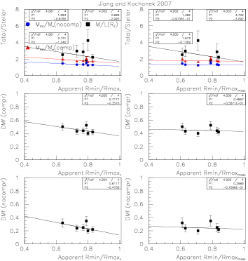
(with adiabatic compression),
(with adiabatic compression),
(without adiabatic compression),
(without adiabatic compression),
(with adiabatic compression),
(with adiabatic compression),
(without adiabatic compression),
(without adiabatic compression).
The analysis assumes spherical symmetry and no uncertainties were
provided. For our global analysis, we used the
and results with compression (favored in [59])
and we assigned them to group 2 reliability.
For information:
,
.
9.11 Keeton, Kochanek and Falco (1997)
In [60] Keeton, Kochanek and Falco analyzed 17 strong lensing candidates. The total mass was obtained by using either a SIE model or a Singular Isothermal Sphere with tidal correction (SIS+Shear) model. The SIE model used to model the 2D mass profiles accounts for ellipticity. This implies a correlation between mass profile and ellipticity, with steeper profile galaxies having larger ellipticity. The luminosity profiles were assumed to follow a de Vaucouleur law. The luminosity uncertainty dominates that of . From the 17 galaxies considered in [60], we excluded 2 spiral galaxies (B0218+357 and B1933+503), 3 for which was not given (MG0414+0534, HST12531-2914 and BRI0952-0115), 4 that are clearly influenced by their environments (MG0751+2716, Q0957+561, B1422+231 and MG1131+0456) and 1 that was poorly understood in [60] (B1600+434). We removed galaxies B0712+472 and MG1549+304 that have a velocity dispersion km.s-1 ( are from [103]). We relaxed our selection compared to our standard km.s-1, otherwise only Q0142-100 would have passed selection. We rejected PG1115+080 as it may be peculiar [59] and B1608+656 because it may have a companion. In all, 3 galaxies remained: Q0142-100, HST14176+5226 and MG1654+1346. We used the values computed in the cosmological model. The vs apparent and mass axis ratios are shown in Fig. 37.

The best fits yield:
,
.
The advantage of the analysis is that ellipticity is accounted for.
The specific caveats are that the analysis is dated (for a strong
lensing analysis) and due to the small number of galaxies we had to
relax our standard criteria minimizing S0 and giant elliptical contaminations.
For these reasons, results were assigned to group 3 reliability.
9.12 Koopmans et al. (2006)
Koopmans et al. [65] analyzed strong lensing and photometry data from 15 early-type field galaxies from the SLACS survey. The strong lensing data allowed them to determine the total mass within . The photometry data was used to determine the total density profile by solving the spherical Jeans equations with an assumed form and a Hernquist profile for the stellar density. Calculations were repeated with a Jaffe profile for stellar density in order to assess the model dependence on the choice of stellar profile. For mass deprojection, a SIE model was used and the mass axis ratio was deduced with precision better than 10%. A systematic study of uncertainties was carried out. There are 4 main sources of uncertainty. The unknown stellar velocity anisotropy has small effects, as does the influence of neighboring galaxies. The choice of model for the stellar and mass densities produced an uncertainty acceptable within the accuracy level of the data. The authors argued that the effect of the halo ellipticity on their study (dark matter fraction variation with radius) is small. We rejected 3 lenses identified as S0 in [2], excluded 2 galaxies with and one with km.s-1. In all, our final sample comprises 9 galaxies. The vs axis ratio, is shown in Fig. 38. We rescaled the uncertainty provided by the authors so that for the best fits. they yield:
,
.
Specific caveats are some model dependence, in particular in the choice
of density profile which was argued to be unphysical in [46]
and spherical symmetry was assumed (except for mass deprojection).
The analysis has the advantages that systematic uncertainties and
model dependence were studied and argued to be under control. Furthermore,
care was taken in choosing and verifying that the galaxies are isolated.
We assigned the results to group 1 reliability.

9.13 Leier (2009)
In [71], Leier analyzed 19 strong lenses with available photometry from the SLACS and CASTLE surveys. The lensing data were used to assess the projected total mass . From it and luminosity data, at was extracted ( is of the same order as for most lenses). was used with the virial theorem to form a velocity dispersion . It agrees generally well with the observed one, , indicating that these galaxies are virialized. We rejected two galaxies for which data are not available (CFRS03.1077, HST14176), one known spiral (Q2237+656)777It has also one of the two worst ratio, , indicating it may not be well virialized., two galaxies identified as S0 in [2], one with significant interaction and classified as peculiar in [59] (PG1115+080, which has and so may not be well virialized), one with significant contribution from its cluster (Q0957) and one with a close companion and unreliable axis ratio (B1608+656). In addition, we applied our standard selection to minimize contamination from giant elliptical galaxies and S0, rejecting one high mass galaxy (J0956+510). In all, 8 galaxies constitute our final sample. For all of them and agree within 20%. Uncertainties on were not provided. We estimated them using the uncertainties given for and and assuming a 20% uncertainty on the luminosity. The resulting uncertainties were then scaled so that . The vs apparent axis ratio, shown in Fig. 39, have best fits:
,
.
The two fits agree well, indicating that the virial
and strong lensing methods are consistent and that the galaxies are
virialized.
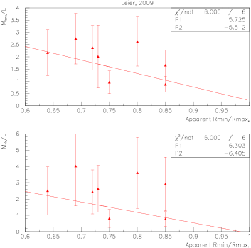
A limitation of this analysis is that spherical symmetry was assumed. The analysis has the advantage that care was taken in choosing virialized galaxies. We assigned the results to group 1 reliability.
9.14 Leier et al. (2011)
In [72], Leier et al. computed the baryon fraction profile for 19 strong lensing galaxies from the CASTLE survey. Lensing and photometry were used to recover the total mass and the mass and light profiles. A Sersic profile was used for stars and the apparent axis ratio was accounted for in the stellar mass calculation. were extracted via a Stellar Population Synthesis model. Various IMF were used with results agreeing within 10%. Ignoring the spiral bulge Q2237, the giant MG2016 and RXJ0911 that is believed to not be a true lens, and applying our standard and km.s-1 criteria, we rejected 13 of the 19 galaxies ( are from [103]). 3 others had to be rejected because of notable interactions with environment, leaving only 3 galaxies (Q0142, Q0047 and MG1104). Slightly relaxing our selection to km.s-1 or km.s-1 provides a sample of 6 galaxies. The vs apparent axis ratio is shown in Fig. 40. The best fit is:
.
The uncertainties were scaled so that the . The caveats
are that in order to get a reasonably sized sample, we relaxed
our selection. Also, like in the other CASTLE lens survey analyses,
the sample is more inhomogeneous, as noted e.g. in [71].
Finally, the axis ratios came from different authors thus possibly
adding point-to-point fluctuations, although this was accounted for
by forcing for the fit. We assigned the results
to group 2 reliability.
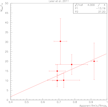
9.15 Ruff et al. (2011)
Ruff et al. [88] analyzed 11 early-type strong-lensing galaxies from the SL2S survey. The lenses have an average redshift of <>=0.5. A SIE model was used to obtain the total mass within . Photometric data were used to compute both the stellar mass , using either a Chabrier or a Salpeter IMF, and the size of the galaxy. An elliptical de Vaucouleur profile was used to obtain the surface brightness. The was calculated at by solving the spherical Jeans equations. No galaxy type identification is given in the article. The requirements that and km.s-1 were used to remove possible S0 and giants. 7 galaxies passed the selection. Mass ratios vs apparent and mass axis ratios are shown in Fig. 41.

The best fits are:
,
,
,
,
,
,
,
,
,
,
The mass ratio uncertainties were scaled so that .
The difference between and is that stands at and the models account for the apparent ellipticity and do not need IMF input. stands at , used models accounting for ellipticity but was obtained solving the spherical Jeans equations with an assumed IMF. For our sample, we have , but with in most cases.
A caveat here is that only a few tentative type identifications are available from [88] so we required km.s-1 and to exclude possible of S0 and giant galaxies. Little indication on the environment influence is given in [88]. Advantages are that ellipticities were accounted for in the mass calculations and the model dependence upon the IMF can be estimated. For these reasons, the results are assigned to group 2 reliability and the and using a Chabrier IMF are assigned to group 3 reliability.
9.16 Treu and Koopmans (2004)
Treu and Koopmans [98] analyzed 5 strong lenses to obtain the distributions of luminous and dark matter within . The galaxies have redshifts 0.5<<1. A SIE model was used to provide a robust estimate of the total mass whilst the luminous mass profile was deduced from stellar dynamics data. Dark and luminous profiles were assumed to be spherical. The dark matter was assumed to follow a NFW profile and the luminous one a Hernquist profile. The lenses were chosen relatively isolated. The authors studied the effects of stellar anisotropy and of neglecting ellipticity and concluded that these effects are small. Applying standard km.s-1 and would have selected only 2 galaxies (0047 and C0302). We slightly relaxed the selection to accept H1417 ( km.s-1). We note that C0302 may belong to a small galaxy group and so subject to environment interaction. The 2 other available galaxies were rejected because one is a giant (MG2016) and the other most probably a S0 (H1543). The best fits to and vs apparent axis ratio, shown in Fig. 42, are
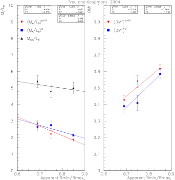
,
and
for which Fundamental Plan assumptions were made to further constrain the data.
The uncertainties from [98] were symmetrized and scaled so that . The reason why has a negative slope and the have a positive one is because drops faster with axis ratio than .
The data were analyzed assuming spherical symmetry but the authors argued that accounting for ellipticities produced little difference. Likewise, the effect of stellar ellipticity was studied and found unimportant. We assigned the result to group 1 reliability.
10 Ellipticity and projection corrections
There are two types of ellipticity corrections. The first one is due to the ellipticity affecting the computation of quantities relevant to our analysis. We call this the “ellipticity corrections” proper and discuss it in the next Section. The second type is correcting for the fact that often only the apparent ellipticity of a galaxy is known, which strongly reduces the correlation we study in this article. We address this correction in Section 10.2.
10.1 Ellipticity corrections
The exact formula to compute depends on ellipticity. Generally, assuming spherical symmetry underestimates . Sensitivity to ellipticity differs for different methods. It is important e.g. for the virial method but less so for the strong lensing method when the total mass is extracted at the Einstein radius and the luminosity is obtained from deprojected data. Except for the strong lensing data for which the correction is expected to be small, the data discussed here at least approximately or partially corrected to account for ellipticity. The caveat is that the correction may be approximate and often uses apparent axis ratio rather than the true intrinsic axis ratio. Hence, it may still not correct fully the .
10.2 Projection correction
This correction is independent of the technique used to extract , as long as the axis ratio distribution of the galaxy sample is also independent of the technique, e.g. a technique does not preferentially choose galaxies with large or small apparent axis ratios. We assume that this is the case and apply the projection correction, unless it was already done in the original publication as e.g. in sections 5.1, 8.1 or 9.2. We use our results from Section 4.1 (Bacon et al. [3]) to estimate this correction since it is the second largest sample of galaxies (the largest sample is that of Prugniel & Simien [84]. However, the authors remarked it could be slightly biased).
For an oblate spheroid viewed at an angle , its real axis ratio relates to its projected apparent axis ratio as [94]:
| (1) |
We can safely assume that the galaxies in our study are oblate and none are prolate. We assume the distribution to be gaussian, see top left plot of Fig. 43. The characteristics of the gaussian are determined by matching the simulated distribution of apparent axis ratios to the actual distribution of our data sample (bottom left plot). This results in a gaussian centered at 0.55 and with a full width of 0.07. The top right plot shows the assumed correlation between and real axis ratio. The simplest choice is a linear relation. However, it could lead to unphysical (negative) . To circumvent this problem, we can choose a function that is linear for most of the values but flattens near the and limits, e.g. a Fermi-Dirac function. We do the projection correction for both linear (Fig. 43) and Fermi-Dirac functions (Fig. 44) cases in order to estimate the dependence upon the choice of function. The linear function fitting best the observed vs (bottom right plot) is with and . The best fit using a Fermi-Dirac function is for , , and . The bottom left panel shows the observed (red) and simulated (black) distributions of the apparent axis ratio. To obtain the simulated one, the gaussian distribution is transformed using Eq. 1 with the viewing angle randomly chosen between 0 and . A random shift toward larger values is added to reproduce the rounding effect of the resolution of the detector. (If, due to this shift, , we either set it to 1 or redraw a random value for the original ). The bottom right panel displays vs apparent axis ratio. We use events for the fit but for clarity, only the error bars of the first 100 events are shown. The distribution reproduces well the observed one (shown by red symbols). This supports that the dispersion is not only gaussian but mostly comes from the galaxies’ random projections. As done with the observational data, we fit this distribution with a linear form . In the simulation, the uncertainties are proportional to , as for the data. Using a gaussian distribution, we randomly offset the central values of the simulated points on the bottom right figure within their error bars.
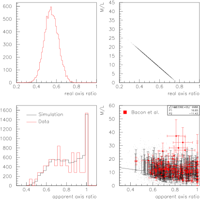
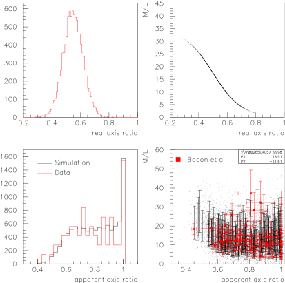
The correction has some model dependence due to the following assumptions:
No prolate galaxies in our sample;
gaussian distribution of the real axis ratios;
The assumed form for the relation between the real axis ratio and ;
The modeling of the detector resolution effect.
Furthermore, it is unclear how to apply the correction because the real axis ratios for
the observed data are unknown and the correction is determined
on statistical basis. Given the distribution
of the real axis ratio (top left panel), it is sufficient to only consider the range
. There, the Fermi-Dirac form is
approximately linear. Averaging the results derived with both forms, the simulation of the projection effect
gives a correction of about for the slope vs axis ratio correlation.
11 Correlations
Many of the quantities describing galaxies are interrelated. Therefore they may indirectly generate correlations with or , some of them spurious: a measurement or observation bias unrelated to and may propagate to one or both of them due to interrelations. We systematically studied this possibility using mostly the galaxy sample from Ref. [3]. We summarize our findings in this section. The detailed analysis can be found in Appendix L. Using the galaxy sample from [3] is convenient due to its large statistics and the relatively large number of galactic characteristics provided. They are:
-
•
The ratios obtained from three different virial estimates.
-
•
The apparent effective radius, (given in arcsec).
-
•
The absolute effective radius, (given in Kpc).
-
•
The apparent axis ratio, .
-
•
The galactic surface brightness, .
-
•
The central velocity dispersion, .
-
•
The distance modulus, , for each galaxy.
-
•
The galactic absolute blue magnitude, .
-
•
The galactic integrated apparent blue magnitude, .
Furthermore, we also used galaxy samples other than that of Ref. [3] to check correlations with galactic characteristics other than those just listed.
That Ref [3]’s data are dated is not an issue because the selection criteria
keeps only galaxies with characteristics agreeing with the NED ones, which are current.
Furthermore, older data are presumably more contaminated with measurement or
observation biases, and therefore, they are better suited to study spurious correlations
and provide a useful upper limit for these biases. In other words, while
the older data may be less sensitive to an actual vs
correlation because it would be diluted by jitters and worst resolutions, they are more
sensitive to spurious correlations and if an upper limit for those is determined to not be large,
the genuine origin of the vs correlation can be validated.
Three types of interrelations are possible:
I) Relations of well-understood origin, e.g. that between
and originating from the virial theorem, or the reduction of apparent sizes and luminosities
as the distances from the galaxies to Earth increase.
II) Relations known Phenomenologically, e.g. the Kormendy [66] and Faber-Jackson [41]
relations.
III) Unknown relations.
We looked for correlations for all the combinations between pairs of characteristics by linearly fitting them, a non-zero fit slope indicating a correlation. We directly used the uncertainties given in Ref. [3] (no rescaling according to the unbiased estimate). We clearly confirmed all known relations (types I and II above) except for the surface brightness vs absolute blue magnitude relation, which was reported in [10]. The correlation is seen, yet not as strongly as for the other known relations. We found several other relations. They are weaker and are either resulting from known relations, or possibly due to measurement or observation biases. All these relations are pictured in Fig. 45.
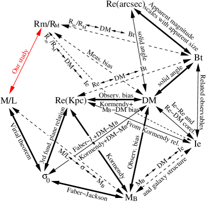

We remark that without applying the selection criteria described in Section 3.1, other relations than those indicated on Fig. 45 should have been present. It is known, e.g., that small galaxies are prone to be flatter, indicating a correlation between and (Kpc). Or that the of giant and dwarf galaxies tend to be larger, indicating a correlation between and (Kpc). Furthermore, giant and dwarf galaxies tend to be rounder indicating a correlation between and . Such correlations would have obscured the present study and this provides another reason for implementing the selection criteria of Section 3.1
Fig. 45 shows that there is no direct relations between both and and a third characteristic. This precludes (at least for sample [3]) that the vs correlation is a indirect consequence of interrelations between some of the other 7 galaxy characteristics in Fig. 45. Yet, the other relations may still somewhat contribute to the vs correlation via multiple steps, e.g. . We discuss this possibility in section 11.1.
Beside the interrelations between the galaxy characteristics listed in [3], we also checked, using the sample of Ref. [69], the effect of the known correlation between metallicity and . Since no correlation was found between and , the - correlation should not affect . Also, a relation between and the luminosity density was signaled in [69]. We confirmed it but saw no correlation between and thus, again, this should not affect .
11.1 Measurement bias study
Fig. 45 shows that all the weak correlations suggestive of
measurement biases are associated with .
This calls for studying the influence of on .
To do so we used again the galaxy sample [3].
was binned and plotted for each bins.
A linear fit of vs yields a non-zero positive
slope of (). This indicates that, once a bias is corrected for,
would increase by a factor of .
However, since this relies on linearly extrapolating over 31 units using a fit just done over 4.5 units,
we decided to not correct . Supporting this conservative
choice are the facts that:
I) It is unclear if the bias is real, the fit slope being just 1.6 from zero;
II) the errors on the extrapolation are large;
III) This bias cannot be at the origin of the correlation we are studying since the correction
would decrease it.
12 S0 contamination study
It is often delicate to distinguish between S0 galaxies and elliptical galaxies with large axis ratios. Such -dependent contamination could cause the decrease of with reported in Section 13 because tends to be smaller for S0 than for elliptical galaxies. If so, the correlation’s origin would not be physical but a systematic bias in galaxy classification. The strict generic rejection criteria described in section 3.1.1 suppress that contamination because they systematically exclude galaxies of unclear/transitional morphologies, namely E/S0, E+ or E? types (E+ are “late elliptical galaxies”, a transition stage between E and S0) since those may be more prone to misclassification. Furthermore, effects of a S0 contamination would would emerge in the systematic studies, specifically varying the strictness of the S0 rejection criteria cf. Section 12.1, the study of how the vs with depends on cf. Section 12.5 and apparent magnitude cf. Section 12.6, and investigating a possible vs correlation (cf. Section 12.4 and appendix B).
We discuss here these specifics tests. They indicate that S0 being at the origin of the correlation is unlikely.
12.1 Independent S0 rejection criterion
A standard method to check the efficiency the main rejection criterion and the consequence of a possible contamination is to add an independent rejection criterion and varies its strictness. To do this, to the primary criterion (based on the NED classification) we added a second one consisting of rejecting low velocity dispersion galaxies, as S0 tend to have lower velocity dispersion values. These two rejection criteria are independent in the sense that any rejection inefficiency of one criterion is unrelated to the inefficiency of the other criterion.
Applying the second rejection criterion results in a correlation agreeing with
the nominal analysis. This test is done on the largest sample of galaxies
(112 galaxies, of which 44 pass the second criterion) so it is statistically
significant. A possible issue is that the second criterion might
bias the correlation e.g. because of the proportionality between and velocity
dispersion. The average value of is in fact smaller once the second criterion is
applied. To compensated for this, we increased uniformly those
so that their average matches that of the nominal analysis.
If S0 contamination was biasing the nominal analysis,
an agreement between the nominal and second analyses
could still occur if:
1) a new effect emerged from introducing the second criterion, and
2) that effect mimics the (now suppressed) S0 contamination effect.
Such coincidence being unlikely, this check attests the reliability of the nominal rejection criterion.
Another such misleading agreement between the nominal and second analyses
could also occur if S0 and E display similar
vs correlations888
Such possibility appears
to be ruled out by other checks performed in this manuscript.. If so, our check would not
be able to assess the S0 contamination. However, this one would then have no influence on our final result.
12.2 Consequence of a S0 contamination for galaxy census
In this section, we assume that the vs correlation reported in this document stems S0 contamination, and we investigate the consequence on galaxy type census. To reduce possible systematic bias, we conducted the analysis on large samples of data determined either with the virial theorem [84] or from lensing [2]. Our analyses (described next) conclude that assuming that the correlation is due to S0 contamination would lead to a proportion of E and S0 galaxies clearly conflicting with the observed census.
12.2.1 Analysis using virial data (Prugniel & Simien data set)
We use here data from Prugniel & Simien [84]. From those, (see table of Section K). At small values of , S0 contamination is suppressed since S0 are highly flattened. Thus, the value of at offers a clean value of . Our work hypothesis here being that for elliptical galaxies is independent of , we have under this hypothesis .999This is the value prior to the projection correction discussed in Section 10.2. This correction should in principle be implemented but, since it is proportionate to the physical correlation assumed here to not be present, the correction has no effect. We have a lower bound for because, to be consistent with the assumption that S0 contamination produces the correlation seen over the full span of , there must be some remaining S0 contamination at .
To determine the mass-to-light ratio for S0, , we apply a similar procedure as that for elliptical galaxies. We keep only good S0, rejecting dwarf or peculiar S0, S0 listed in the Arp catalog, E/S0, S0?, SB0 (because a visible bar would surely identify a S0, even if it is face-on, which then would be rejected and unable to contaminate the elliptical galaxy sample), BrClg, etc. We obtain a set of 24 S0 with an average . Using a subset of S0 with to avoid possible E contamination, the average becomes .
Supposing that and are independent of , and that a S0 contamination causes a correlation, imply a contamination , where is the value of at which the S0 contamination is supposed to become negligible, and is the ratio of misidentified S0 over the total amount of assumed elliptical galaxies. Results vs are displayed in Fig. 46. Clearly, the putative contamination would have to be implausibly large to account for the observed vs correlation. For instance, it would imply that all round () elliptical galaxies that we used in this analysis are in fact S0 misclassified as ellipticals. Even the rather conservative 2 lower bound of the error band in the bottom panel of Fig. 46 implies a large , signifying that over half of the apparently round elliptical galaxies are misidentified and in fact are S0. Considering that of a set of disks oriented randomly would have , together with the fact that in the observed distribution of ellipticals, of the galaxies identified as ellipticals have (see e.g. Fig. 43), then the ratio of S0 to elliptical galaxies should be 7-to-1. Although estimated conservatively, this still disagrees with the censuses that indicate a similar number of elliptical and S0 galaxies [15]. We conclude that a S0 contamination cannot be the origin of the vs correlation.
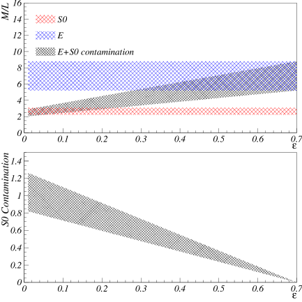
12.2.2 Analysis using lensing data (Auger et al. data set)
The Prugniel & Simien data [84] are obtained using the virial theorem. We repeat here the analysis with the Auger et al. data [2], obtained using gravitational lensing for which the mass estimate procedure is generic to both E and S0. From these data, . We conservatively use the largest correlation (, and extracted using a Chabrier IMF), . Selecting S0 from the set [2], we obtain a subset of 5 S0 (we rejected 2 E/S0). From this sample, we obtain a vs correlation slope of . The deduced putative contamination is shown in Fig. 47. It is similar to the one obtained from virial data and so the same conclusion applies.
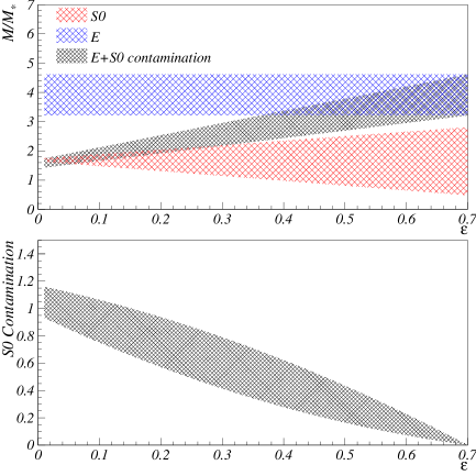
12.3 Case of the S0 contamination at small only
In sections 12.2.1 and 12.2.2, the S0 contamination was chosen to dependent linearly with in order to reproduce the linear dependence of with . However, this linear dependence stems from our choice of the fit function, which we chose to be linear as it is the simplest assumption, see Section 3.2. If S0 contamination were in fact at the origin of the vs correlation, it could be due e.g. to a large S0 contamination presents solely about . If so, higher order polynomials would fit the data better. whilst this is not the case we nevertheless, for completude, investigate here this possibility.
If a (i.e, face-on S0 ) S0 contamination were significant, removing these galaxies from the analysis should significantly decrease . This prediction was investigated with the highest statistics data set of Prugniel & Simien [84]. Excluding galaxies with decreases the sample from 102 to 76 galaxies and yields . This is compatible with the nominal value of and is, if anything, steeper than the nominal value in contrast to what we would have expected from face-on S0 contamination.
It is also immediately evident from any high statistics correlation plots, e.g. Fig. 1, that excluding galaxies with high would not modify significantly .
12.4 Stellar ratio vs ellipticity study
We investigate in appendix B the possibility of a vs ellipticity correlation. No such correlation was found. However, just like for , the stellar ratios tend to be smaller for S0: Ref [19], reports that low velocity dispersion early-type galaxies, i.e, galaxies more likely to be S0, have of about 2 . High early-type galaxies, i.e, those more likely to be ellipticals, have of about 4 .101010Similarly, in [17], it is shown that fast rotators have a smaller (about 1.5 to 3 ) than slow rotators (about 2.5 to 3.5 ). If fast rotators tend to be S0, then S0 tend to have smaller than elliptical galaxies. Consequently, if S0 contamination were at the origin of the vs ellipticity correlation, it would also produce a vs ellipticity correlation, which is not seen. This further rules out the possibility that S0 contamination is at the origin of the correlation.
12.5 Correlation with distance moduli
If the vs correlation were due to contamination from S0, then its slope should be steeper for distant galaxies because they are harder to classify. However, Fig. 49 shows that this is not the case: the obtained using the strong lensing method pertain to distant galaxies, yet their are similar (in fact slightly lower in average) to that obtained with the virial theorem, typically applied to local galaxies. Furthermore, a contamination from S0 would cause an increase of with distance modulus, yet there is no evidence of such increase, see page L.3.2.
12.6 Correlation with apparent magnitude
Following the same argument as in the previous section, a contamination from S0 would cause to be inversely dependent on apparent magnitude because fainter galaxies are harder to identify. The apparent magnitude being strongly correlated with distance modulus, the conclusion of section 12.5 should directly apply. Nevertheless, we investigate explicitly here the possible correlation between (or equivalently ) and apparent magnitude. We grouped the in seven equidistant bins of , the integrated apparent blue magnitude, and then extracted for each bin the slope . The result is shown in Fig. 48. There is no increase of with . The best linear fit to the data yields . As expected from the strong correlation between and distance modulus, there is a hint of effect opposite to what should have been expected from a S0 contamination, i.e, a possibly negative slope .
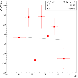
13 Global results
The results of sections 4 to 9 can be combined to extract , the average slope of vs axis ratio. Several points require caution:
-
•
whilst are most often estimated in the B-band, not all of them are. Another scaling factor occurs between using different Hubble parameter values. Lastly, some results are expressed as instead of . We assume here that . To address these points, we impose =8. We choose to normalize to 8 as it is a typical value for of elliptical galaxies. The choice corresponds to where the distribution of elliptical galaxies peaks, which makes extrapolations unnecessary, in contrast to choosing other values such as e.g. .
-
•
Some results use similar methods to obtain and share a number of the same galaxies in their sample. Thus, these results can be highly correlated, biasing the average. Furthermore, some results are, in the context of our study, less reliable than others. This is addressed by applying the following procedure:
-
–
The uncertainty is scaled by the reliability factor from 1 (most reliable) to 4 (least reliable).
-
–
For extractions using a similar method, grouped in Sections 4 to 9, we identify the number of shared galaxies and increase each uncertainty assuming that the uncertainty is statistically dominated. This procedure accounts also for the difference in reliability factors between analyses because results are weighted by them when combined. Uncertainties on results using shared galaxies are multiplied by 1.3 to 6.1 for the virial methods, by 1.2 to 2.0 for the stellar modeling method, by 1.1 to 2.1 for the PNe and CG method, by 1.2 for the X-ray and disk methods and 1.2 to 6.2 for the strong lensing method (except for [60] which is fully weighted out as it employs only galaxies used by more reliable analysis). For this procedure, one must assume that analyses employing the same method and the same galaxies are exactly correlated. This is not true as a particular analysis uses different assumptions, IMF, profiles, etc… Particular analyses also vary in their details and the quality of the data differs since the results have been published over a 30 years range. Hence, our correction is conservative, yielding overestimated uncertainties. This is partly alleviated by fitting vs radius with a constant and scaling the uncertainties so that .
We note that, whilst important, this procedure happens to numerically have a small influence.
-
–
-
•
When the results of an analysis are provided for different IMF, we choose the result using a Chabrier IMF because, with the Salpeter one, it is the most commonly used IMF whilst being more recent than Salpeter’s.
-
•
With the strong lensing method, can be extracted using apparent or mass axis ratios. We prefered using the apparent axis ratio rather than the mass one for several reasons:
-
–
The mass axis ratio is more model dependent.
-
–
It is not systematically calculated in the articles, although it can be obtained from other works using the same galaxies. However, its is desirable for consistency to use mass axis ratio obtained using the same model and assumptions as used for the extraction. We remark that, apart for Grillo et al. [53], the vs axis ratio correlation is always stronger for mass axis ratio, i.e, . It may be because reflects better the intrinsic axis ratio, or it could be a systematic effect of the lensing method since this one does not fully account for ellipticity effects.
-
–
-
•
We globally rescale the uncertainties so that for vs radius, . (We use a one-parameter fit, viz is assumed to be independent of radius.) Forcing is justified since many different methods were used to obtain the with either uncorrelated systematic uncertainties, or, for using the same extraction method, we accounted for the correlation of the results.
Fig. 49 displays the slopes .
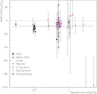
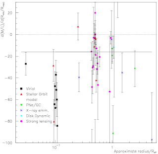
For clarity, they are shown vs the approximate average value of the radius at which a is extracted. The average slope before the projection correction describe in Section 10.2 is:
, and
after correction111111The result is not approximately times larger, as was obtained in Section 10.2, since the additional uncertainty from the projection correction is proportional to the slope. Thus, the contribution to points near is smaller and their relative weight in the averaging procedure increases. .
Note: accounting for the reliability of the methods and for correlations between the various results is methodologically important but this happens to not change significantly the results. Without it, before projection correction, to be compared to with it.
These results assume that is constant with radius .
Fig. 49 reveals that combined results from different methods have systematic shifts, especially between the virial and the strong lensing combined results. This could come from the fact that different methods estimate at typically different radius values: in fact, it has been reported that at smaller radii, the baryonic mass dominates over the dark one [9, 16, 67, 74, 78, 79, 97, 104]. In other words, the values increase with radius. In our analysis however, all values are normalized to 8, which effectively removes the dependence on which particular radius value is used to obtain . However, this introduces an artificial radius dependence of since this one scales with the factor used to normalize to 8, that factor itself depending by definition on the value of the extraction radius. This artificial dependence is opposite to the actual dependence of with radius, i.e. decreases with , see Fig. 49. To fix this issue, we use a normalization derived from the results of Ref. [16],
| (2) |
to include the -dependence of . Fig. 50 displays obtained with Eq. (2) normalization. Compared to Figs. 49, the -dependence of in Fig. 50 has decreased. To completely cancel it, a factor of 3 to 4 (rather than 1.7 in Eq. 2) would be needed. As this larger factor remains compatible with the dependence derived from Ref. [16]’s data, the -dependence seen in Fig. 49 may originate fully from the -dependence of . Nevertheless, other effects could contribute to the systematic differences noticed in Fig. 49. For example, the less stringent selection applied to the distant galaxies used with the strong lensing method could result in a contamination that reduces the correlation. Furthermore, the extracted with the strong lensing method have no ellipticity correction since the method is less sensitive to . Actually, we remark that if is used instead of , the ellipticity-corrected virial results and the strong lensing one would agree.
13.1 Results
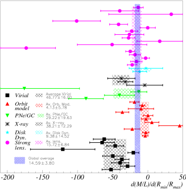
Fig. 50 shows that the averaged obtained using the six different methods are all negative and average to . The uncertainty stemming from the -dependence of the normalization is conservatively estimated from the difference between the two results obtained with the dependent normalization and with the constant one. With this additional uncertainty accounted for, the final result of the analysis is
| (3) |
This signals a statistically meaningful correlation between and . The slope (3) is proportional to the normalization , see Eq. 2. The slope (3) is large compared to 7.7. We remark that if the galaxy selection criteria had not been applied, the correlation would vanish, diluted by large fluctuations. This may account for the fact that the correlation had not been identified earlier. The analyses of Ref [19, 20] e.g. did not find evidence of this correlation. However, whilst they analyzed a large galaxy sample (260 galaxies), only of those galaxies are bona-fide elliptical galaxies, and are lenticular or spiral galaxies. Similarly, we checked using the data [3] that when selection is not applied, the correlation vanishes.
14 Summary and conclusion
We investigated the possibility of a correlation between the dark matter content of elliptical galaxies and their ellipticity. Elliptical galaxies can differ importantly from each other, and peculiarities might bias the estimation of the dark mass, causing systematic and random variations. Therefore, it was important to select a large and homogeneous sample of galaxies. Effects of the peculiarities are then minimized by the homogeneity and suppressed statistically. Furthemore, since the value of depends on the galactic radius at which the ratio is extracted, as well as on the wavelength at which the galaxy luminosity is calculated (typically the B-band, but not always), it was necessary to normalize the at a given to a unique value. We chose and there, used the typical value . With this normalization, we found a clear correlation: . The dark matter information is obtained from six different approaches (virial theorem, stellar orbit modeling, orbits of planetary nebulae and globular clusters, embedded disk dynamics, hydrostatic equilibrium, and strong lensing) to minimize methodological bias. Possible effects of measurement or observation biases were studied thoroughly. Furthermore, we repeated the same analysis on the stellar , see appendix B, and no significant correlation with ellipticity was found, as it should be. This suggests that our procedure is free of significant biases. Possible conclusions are either that:
-
1.
There is a surprisingly strong influence of the dark matter halo on a galaxy shape, possibly from the halo shape as suggested by the stronger correlation generally seen when investigated with mass axis ratio rather than apparent (project luminous) axis ratio. This would allow us to experimentally address the question of the shape of the dark halo and be critical to understand galaxy formation.
-
2.
The dynamical evidences from which the dark matter content of galaxy is inferred are misinterpreted. In fact, the impulse for the present study originated from a prediction from Ref. [31] (see also Refs. [33, 36]). In this framework, if a homogenous system is locally dense enough so that in that location, the non-linearity of General Relativity are non negligible, this system should display a correlation between its dynamical total mass analyzed using Newton’s law of gravity (in our case, the galaxy dark mass) and its asymmetry (in our case, the galaxy ellipticity). Beside the present correlation, this effect also explains [35] the correlation between dynamical and baryonic matter accelerations observed in Ref. [76]. Finally, it provides an explanation for the origin of dark energy: it emerges from the Universe inhomogeneities and anisotropies [34].
-
3.
There is a significant bias in the data and/or methods, in which case they cannot be trusted to estimate accurately the dark matter content of elliptical galaxies. However, our thorough investigation of the various inter-dependences of the variables characterizing an elliptical galaxy reasonably suggests that this correlation is physical rather than a methodological, observational or measurement bias.
Finally, a practical use of the correlation is that once the total galactic mass is known the true ellipticity of the galaxy can be directly deduced.
Acknowledgment This research has made use of the NASA/IPAC Extragalactic Database (NED) which is operated by the Jet Propulsion Laboratory, California Institute of Technology, under contract with the National Aeronautics and Space Administration.
References
- [1] M. W. Auger et al. ApJ 705 1099 (2009)
- [2] M. W. Auger et al. ApJ 724 511 (2010)
- [3] R. Bacon, G. Monnet and F. Simien, A A 152 315 (1985)
- [4] M. Barnabe et al. MNRAS 399 21 (2009)
- [5] M. Barnabe et al. MNRAS 415 2215 (2011)
- [6] R. Bender et al. AA 217 35 (1989)
- [7] G. Bertin et al. AA 292 381 (1994); R. P. Saglia et al. ApJ 403 567 (1993)
- [8] F. Bertola et al. ApJ 373 369 (1991)
- [9] F. Bertola, A. Pizzella, M. Persic and P. Salucci. ApJ 416 45 (1993)
- [10] B. Binggeli, Proc. ESO/OHP Workshop on Dwarf Galaxies, ed. G. Meylan, & Ph. Prugniel, 13 (1994)
- [11] See. e.g. J. Binney and S. Tremaine, Galactic Dynamics. Princeton University Press; (2008)
- [12] A. S Bolton et al. ApJ. 682 964 (2008)
- [13] F. Brighenti, W. Mathews ApJ 486 L83 (1997)
- [14] G. Bruzual and S. Charlot MNRAS 344, 1000 (2003)
- [15] Calvi R., Poggianti B. M, Fasano G., Vulcani B., MNRAS 419, L14 (2012)
- [16] M. Capaccioli, N. R. Napolitano and M. Arnaboldi, astro-ph/0211323 (1992)
- [17] M. Cappellari et al. MNRAS 366 1126 (2006)
- [18] M. Cappellari et al. ApJ 704 L34 (2009)
- [19] M. Cappellari et al., MNRAS, 432, 1709 (2013)
- [20] M. Cappellari et al., MNRAS, 432, 1862 (2013)
- [21] V. F. Cardone, C. Tortora, R. Molinaro and V. Salzano AA 504 769 (2009)
- [22] V. F. Cardone, A. Del Popolo, C. Tortora, and N.R. Napolitano MNRAS 416 1822 (2011)
- [23] C. M. Carollo and I. J. Danziger MNRAS 270 523 (1994); MNRAS 270 743 (1994)
- [24] C. M. Carollo et al. ApJ 441 25 (1995)
- [25] G. Chabrier PASP 115 763 (2003)
- [26] K. H. Chae, S. Mao and P. Augusto MNRAS 326 1012 (2001)
- [27] L. Coccato et al. MNRAS 394 1249 (2009)
- [28] C. Conroy and P. G. van Dokkum ApJ 760 71 (2012)
- [29] P. Das et al. MNRAS 402 1362 (2010)
- [30] A. J. Deason et al., ApJ 748 2 (2012)
- [31] A. Deur, Phys. Lett. B 676, 21 (2009)
- [32] A. Deur, MNRAS 438, 2, 1535 (2014)
- [33] A. Deur A, Eur. Phys. J. C 77, 412 (2017)
- [34] A. Deur, Eur. Phys. J. C 79, 883 (2019)
- [35] A. Deur, C. Sargent and B. Terzic, ApJ 896, 2 94 (2020)
- [36] A. Deur, [arXiv:2004.05905 [astro-ph.GA]].
- [37] S. Djorgovski and M. Davis, ApJ 313 59 (1987)
- [38] A. Dressler, et al. ApJ 313 43 (1987)
- [39] G. de Vaucouleur, Annales d’Astrophysique 11 247 (1948)
- [40] S. di Serego Alighieri et al. AA 442, 125 (2005)
- [41] S. M. Faber and R. E. Jackson, ApJ 204 668 (1976)
- [42] C. D. Fassnacht and J.G. Cohen, ApJ 115 377 (1998)
- [43] C. Faure et al. ApJ 176 19 (2008)
- [44] C. Faure et al. AA 529 A72 (2011)
- [45] H. C. Ferguson et al. ApJ 600 L107 (2004); I. Trujillo et al. ApJ 604 521 (2004); A. W. Zirm et al. ApJ 656 66 (2007); A. Cimatti AA 482 21 (2008); I. Damjanov et al. Ap.J 695 101 (2009).
- [46] I. Ferreras, P. Saha and L. R. Williams ApJ 623 5 (2005)
- [47] I. Ferreras, P. Saha and S. Burles MNRAS 383 857 (2008)
- [48] C. Foster et al. NMRAS 415 3393 (2011)
- [49] Y. Fukazawa et al. ApJ 636 698 (2006)
- [50] R. Gavazzi et al. arXiv:1202.3852 (2012)
- [51] K. Gebhardt et al. ApJ 583 92 (2003)
- [52] C. Grillo et al. AA 477 25 (2008)
- [53] C. Grillo et al. AA 501 461 (2009)
- [54] L. Hernquist, ApJ 356 359 (1990)
- [55] B. P. Holden et al. ApJ, 620 83 (2005)
- [56] P. J. Humphrey et al. Proceedings of “The X-ray universe 2005”, A. Wilson Ed. (2005)
- [57] P. J. Humphrey et al. ApJ 646 899 (2006)
- [58] N. Jackson et al. AA 334 33 (1998)
- [59] G. Jiang and C. S. Kochanek ApJ 671 1568 (2007)
- [60] C. R. Keeton, C. S. Kochanek and E. E. Falco ApJ 509 561 (1998)
- [61] D. D. Kelson et al. ApJ 531 184 (2000)
- [62] L. J. King et al. NMRAS 295 41 (1998)
- [63] E. Komatsuet al., Astrophys. J. Suppl. 192 18 (2011)
- [64] L. V. E. Koopmans et al. NMRAS 303 727 (1999)
- [65] L. V. E. Koopmans et al. ApJ 649 599 (2006)
- [66] J. Kormendy, ApJ 218 333 (1977)
- [67] A. Kronawitter et al. AA 144 53 (2000)
- [68] P. Kroupa, C. A. Tout and G. Gilmore NMRAS 262 545 (1993)
- [69] T. R. Lauer ApJ 292 104 (1985)
- [70] J. Lehar et al. ApJ 536 584 (2000)
- [71] D. Leier MNRAS 400 875 (2009)
- [72] D. Leier et al. ApJ 740 97 (2011)
- [73] J. Magorrian et al. ApJ 115 2285 (1998)
- [74] J. Magorrian and D. Ballantyne NMRAS 322 702 (2001)
- [75] C. Maraston NMRAS 362 799 (2005)
- [76] S. S. McGaugh, F. Lelli, and J. M. Schombert, Phys. Rev. Lett., 117, 201101 (2016)
- [77] A. More et al. ApJ 734 69 (2011)
- [78] R. Nagino and K. Matsushita AA 501 157 (2009)
- [79] N. R. Napolitano et al. NMRAS 357 691 (2005)
- [80] N. R. Napolitano et al. MNRAS 393 329 (2009)
- [81] J. F. Navarro, C. S. Frenk and S. D. M. White ApJ 463 563 (1996)
- [82] E. O’sulivan, A. J. R. Sanderson and T. J. Ponman NMRAS 380 4 1409 (2007)
- [83] A. Pizzella et al. AA 323 349 (1997)
- [84] Ph. Prugniel and F. Simien AA 309 749 (1996)
- [85] R. N. Proctor et al. MNRAS 398 91 (2009)
- [86] A. Rettura et al. AA 458, 717 (2006)
- [87] A. J. Romanowsky et al. Science 301 1696 (2003)
- [88] A. Ruff et al. ApJ 727 96 (2011)
- [89] E. E. Salpeter ApJ 121 161 (1955)
- [90] R. P. Saglia, G Bertin and M. Stiavelli ApJ 384 433 (1992)
- [91] R. P. Saglia et al. ApJ 403 567 (1993)
- [92] M. Schwarzschild ApJ 232 236 (1979)
- [93] J. L. Sersic BAAA 6 41 (1963)
- [94] See. e.g. L. S. Sparke & J. S. Gallagher, Galaxies in the Universe. Cambridge University Press (2007)
- [95] T. S. Statler et al. AA 121 244 (2001)
- [96] S. H. Suyu et al. ApJ 750 10 (2012)
- [97] J. Thomas et al. NMRAS 282 657 (2007); NMRAS 415 545 (2011)
- [98] T. Treu and L.V.E. Koopmans, ApJ 611 739 (2004)
- [99] T. Treu et al. ApJ 690 670 (2009)
- [100] G. Trinchieri, G. Fabbiano, D.-W Kim AA 318 361 (1997)
- [101] R. B. Tully and J. R. Fisher AA 54 661 (1977)
- [102] A. van der Wel et al. ApJ 631 145 (2005)
- [103] G. van de Ven, P. G. van Dokkum and M. Franx MNRAS 344 924 (2003)
- [104] R. P. van der Marel MNRAS 253 710 (1991)
- [105] R. P. van der Marel and P. G. van Dokkum ApJ 668 738 (2007)
- [106] R. P. van der Marel and P. G. van Dokkum ApJ 668 756 (2007)
- [107] P. G. van Dokkum and S. A. Stanford ApJ 585 78 (2003)
- [108] G. A. Wegner et al. ApJ 144 3 (2012)
- [109] COSMOS ApJ Supplement Series 172 (2007)
- [110] http://nedwww.ipac.caltech.edu/
- [111] http://nedwww.ipac.caltech.edu/level5/Arp/Arp_contents.html
- [112] In Fukazawa et al. [49] galaxies are grouped into 3 classes: EXG (bright X-ray) CXG (faint X-ray) and VCXG (very faint X-ray) galaxies. VCXG galaxies show signs of disturbed hydrostatic equilibrium and the hot EXG gas property merges with the extragalactic gas of the group/cluster, indicating influence from the environment. Likewise, the galaxies in Nagino and Matsushita [78] are classified in two groups: one consisting of galaxies with their ISM temperature profile constant or decreasing with growing radius (XC group), and the other group made of galaxies of increasing temperature profile (XE group). They surmise that the ISM of the XE galaxies is influenced by the group/cluster hot gas. (Similar conclusions are obtained in by Fukazawa et al. [49].) The second group corresponds to the large massive EXG galaxies in [49] (although there is no perfect 1 to 1 correspondence). For the same reason as for cD or BrClG galaxies, we exclude EXG and XE galaxies from our analysis.
- [113] Without such selection criteria, the best linear fit of the [3] data, as discussed in Fig. 67, to the full data set has no significant slope: . This is understood as coming from the additional jitter caused by the wider characteristics of the galaxies and by systematic biases. For example, a systematic bias stems from galaxies now known to be disc galaxies. The of those mis-identified galaxies is wrong because the virial method does not apply. Their is generally very small, e.g. 3.6 for the SA0 galaxy NGC6909, but their apparent is likely to be small e.g. 0.5 for NGC6909. Thus, these disc galaxies introduce an unphysical bias to the correlation and should be excluded.
Appendix A Other data
Other works studying the dark matter content for several elliptical galaxies can be found in the literature. We list them here, in alphabetical order, for completeness and state why they were not used in the present analysis:
-
•
Bertin et al. (1994) and Saglia et al. (1993). The two articles are from the same group and use the same method. We may thus combine the two data sets without introducing a systematic bias. The authors estimate using two models to fit stellar dynamics (model 2C: 2 components method and model QP: quadratic programming method) for 9 elliptical and lenticular galaxies. Applying our usual selection criteria and relying on NED for the galaxy type and , only 2 suitable elliptical galaxies remain after rejecting E+/cD, S0, SA0 galaxies and NGC7144 since no realistic modeling for this galaxy was achieved. The two remaining galaxies are E0, with too little lever arm to obtain a meaningful vs ellipticity relation. If we keep in addition the 3 cD galaxies, the fits to the vs ellipticity indicate a correlation, see Fig. 51. The best fit result for the 2C method gives . The best fit result for the QP method gives . The respective are 1.5 and 4.6. This data set has a number of caveats: the data are dated (1994). The are not estimated at the same relative radius (they are estimated at around , with 0.8). No uncertainties are provided. We assumed 25% point-to-point uncertainty as this seems to be typical for such study. This leads to 2C and QP results that are compatible with each others, which indicate that 25% is reasonable. The span is small (0.8< <0.96), making the slope extracted from the fits less accurate. Finally, the statistics are limited (5 galaxies), the models assume spherical symmetry -which introduces a vs bias- and they also assumme no galaxy rotation. The main drawback is that we have cD galaxies in the sample. It explains the strong correlation found: cD galaxies tend to have higher than standard elliptical galaxies and, for this particular sample, the cD galaxies have higher ellipticity. For these reasons, we do not consider these results.
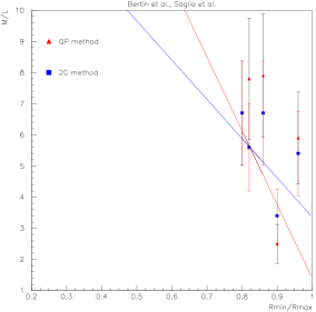
-
•
Barnabe et al. study 6 strong lensing early-type galaxies from the SLACS survey in [4]. This work is superseded by [5] and hence we do not use these results. However, we summarize them briefly: out of the 6 galaxies, we reject one potential giant that has (J0216-0813) and one E/S0 (J0912+0029). The fit to the 4 remaining elliptical galaxies yields and .
-
•
Brighenti and Mathews [13] determine the for 3 early-type galaxies. However, only one is an elliptical. The two others are lenticular galaxies and belong to the Arp catalogue.
-
•
Cappellariet al. [18] provide ratios for 9 early-type galaxies at large redshift . No detailed information on the early-type structure is available. With our standard km.s-1 to minimize S0, we can retain only one galaxy.
-
•
Carollo et al. [24] study the dark matter content of 4 elliptical galaxies but provide only the velocity dispersion profile, without giving the total mass or .
-
•
Carollo and Danziger study 5 elliptical galaxies in [23]. Among them, 3 are SAB, one a SA0 or SApec and one is a cD, leaving only one suitable galaxy.
-
•
Coccato et al. [27] study PNe as tracers for 6 galaxies and add 10 others from the literature. However, only their rotation curves are provided, without total mass or .
-
•
Conroy and van Dokkum [28] construct for 38 early type galaxies. However just a few galaxies pass our selection criteria. Furthermore, only the stellar is provided.
-
•
Das et al. [29] extract mass distributions, circular velocity curves and from the deprojected density and temperature profiles of the hot gas surrounding 6 X-ray bright elliptical galaxies. These extracted quantities are given from the galaxy center to a few (2.5 for NGC4472 to 9 for NGC 1407). The is extracted using the stellar ratio from various references. However, no galaxy passes our standard selection and we thus cannot use these data.
-
•
Fassnacht and Cohen [42] analyze 3 strong lenses from the CLASS survey (B0712+472, B1030+074 and B1600+434). However, the lens velocity dispersions are below our standard km.s-1 criterion, two of them well below. Furthermore B1600+434 is significantly affected by its environment. Hence, the 3 galaxies are not suitable for our study
-
•
Gebhardt et al. [51] provide for 12 early-type galaxies. is obtained for the central region () where stars and central black holes dominate the gravitational potential. Consequently, the model used to infer does not include a dark matter halo and assume instead that the total mass follows light, i.e, is independent of the galaxy radius. This assumption, ruled out by many recent studies, remains reasonable in the radius range studied in [51]. After removing the S0, LINERS, AGN, galaxies for which correlates with the central black hole mass, and Arp galaxies, we are left with only 2 adequate galaxies. Given all these limitations, we did not analyze these data.
-
•
The data from Grillo et al. [52] are not used for two reasons: 1) Grillo et al. model only stellar masses and use the lensing masses from [65]. Since the stellar masses from [52] and [65] agree well, the will be similar to those obtained in [65]. 2) The same group has done a more recent study (Grillo et al. [53]) in which they consider more galaxies and compute both the lensing and stellar masses. This latter work supersedes the earlier results [52].
-
•
Holdenet al. [55] study 4 strong lenses. They belong to a cluster and may be subject to interaction with their environment. In addition two of the lenses are giant elliptical galaxies and a third one has a velocity dispersion of 130 km.s-1, below our standard km.s-1 criterion. We are then left with only one suitable galaxy.
-
•
The two studies from Humphrey et al. [56], [57] employ the same set of 7 early-type galaxies with X-ray data from Chandra. After rejecting galaxies that are peculiar, belonging to the Arp catalog, or being S0/Sy, LINER/Sy, 3 galaxies remain, one of them a LINER. The sample is then too small for a useful study.
-
•
In the work of More et al. [77], 5 strong lensing candidates are analyzed. Out of the 5, one has a S0-like morphology, one is a spiral lens candidate, one might not be a true lens and one yielded inconsistent results, leaving only one potential elliptical candidate.
-
•
Napolitano et al. [79] compile values of for 21 early-type galaxies in order to study the dependence with radius. At small and large radii (typically and several , respectively), is determined using PNe or GC kinematics. is obtained either by fitting modeled orbital distributions to the line of sight velocity distribution or by fitting the velocity distribution profiles using Jeans or similar models. After standard selection insuring undisturbed galaxies we retain only 2 galaxies: NGC821 and 2434. This, with the fact that the data is a compilation of the literature (implying inhomogeneities in the extraction) already used in this article, makes us to not use the results reported in [79].
-
•
Proctor et al. [85] analyze data for 5 galaxies. However, only 2 are adequate elliptical galaxies (E0 and E1-2), with an additional E6?. The authors provide rotation curves but no ratios.
-
•
O’Sullivan, Sanderson and Ponman [82] determine for 3 early-type galaxies. However, only one is an elliptical galaxy, the two others being E+ and S0 galaxies.
-
•
Saglia, Bertin and Stiavelli [90] interpret with their model the photometry and kinematic profiles of 10 galaxies to extract . However, after removing the NELG, cD, E+, peculiar, Seyfert, LERG, NLRG, S0 galaxies and the ones belonging to the Arp catalogue, we are left with only two galaxies, one of them a LINER. This sample is too small for a meaningful study.
-
•
Saglia et al. [91] investigate the presence of dark matter for 3 galaxies. One of them is a RLG, BrClG and LINER and another a E2/S0, Sy2 LINER galaxy appearing in the Arp catalogue. We are then left with only one suitable galaxy.
-
•
di Serego Alighieri et al. [40] compute for 20 early-type galaxies from the K20 survey at large redshift . However, no details are given on the galaxies. We infered the axis ratios visually and, to minimize S0 and giants contamination, applied our standard km.s-1 and criteria. Only 3 galaxies pass this selection, one of them for which we could not determine the axis ratio. is computed using simply the dynamical mass . Such estimate can be easily done for many local galaxies with well established type and characteristics and there is no value in our context to consider an additional few galaxies of uncertain characteristics.
-
•
Trinchieri, Fabbiano and Kim [100] use X-ray data to extract the temperature distribution of the hot gas in 5 early-type galaxies. From it the obtain their . However, after removing the cD, peculiar, S0 galaxies and one belonging to the Arp catalogue, we are left with only one suitable galaxy.
-
•
van Dokkum and Stanford [107] compute for 3 early-type galaxies at large redshift . They belong to the RDCS J0848+4453 cluster. However, the galaxies’ characteristics of are unknown but may be giants, unsuitable in our context. is simply computed as . Such estimate can be easily done for many local galaxies with well established type and characteristics. Considering an additional few galaxies with uncertain characteristics would not add to our study.
Appendix B Correlation between stellar and axis ratio
Since no strong correlation between the stellar ratio and the axis ratio is expected, studying vs should provide a stringent test of our procedure. Among all the data sets considered in this article, 13 of them provide . Here, we describe these sets and the vs correlations derived from them.
B.1 data sets
For all the analyses below except that of Section B.1.3, the uncertainty were taken to be proportional to the values and scaled according to the unbiased estimate. Since the determination of depends on modeling the stellar populations rather than being based on dynamical arguments as for , we do not apply ellipticity corrections to the data (this concerns only the 2 PNe/GC data sets, the other sets had no corrections in the first place). We also do not correct for a possible radius dependence of (see Section 13) because the radius at which the are extracted is usually unspecified (if so we assign a value of , for plotting purpose only). Finally, since the object of the selection criteria is to insure the reliability of the dynamical determination of , these criteria become irrelevant to for . However, since the goal of the vs analysis is to test our primary analysis, we use the same analysis procedure, including applying the selection criteria.
B.1.1 Capaccioli et al.
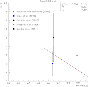
As discussed in Section 6.1, the data were assigned to the reliability group 3. In addition, the is obtained by assuming it to be equal to the calculated central . Consequently, we assign the result to group 4 reliability.
B.1.2 Cappellari et al. SAURON project (2006)
The data and the vs axis ratio analysis are described in
Section 5.1. The fit for the stellar population yields
.
The analysis is assigned to group 1 reliability.
B.1.3 Cappellari et al. ATLAS project (2013).
The data are described in Section 5.2.
The data are from [19]. The best
fit for the stellar population yields
.
The large slope is mostly driven by one single point (NGC 4489), with
especially low , which implies a low uncertainty .
Removing NGC4489 would yield a much smaller slope: ,
but we see no reason to remove it. To avoid the fit to be driven
by the low of NGC 4489, we set the
uncertainties to be constant rather than proportional to .
The resulting fit gives:
,
see Fig. 53.
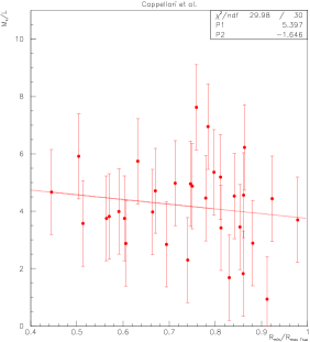
The analysis is assigned to group 1 reliability.
B.1.4 Thomas et al. (2007, 2011) and Wegner et al. (2012)
The data are discussed in Section 5.5, including
the stellar ratios. It was found that:
,
.
The Kroupa IMF results will be used for the global analysis. We assign
the result to group 1 reliability.
B.1.5 Conroy and van Dokkum
These data, discussed in Section A, were not used in the main analysis because only stellar are provided. We show for different bands in Fig. 54.
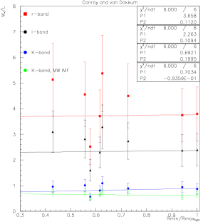
The best fits for the different data are:
for the r-band (with varying IMF).
for the I-band (with varying IMF).
for the K-band (with varying IMF).
for the K-band (with a Milky Way (Kroupa 2001) IMF).
All the fits indicate no ellipticity dependence. We will use
the I-band results when combining with the other publications data.
The analysis is assigned to group 1 reliability.
B.1.6 Deason et al.
The data set is described in Section 6.2. We form .
its correlation with is shown in Fig. 55.
The best fit for the results
derived with a Chabrier IMF yields:
and, for results derived with a Salpeter IMF:
.
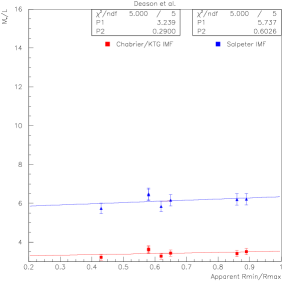
When forming the global result, we will use Chabrier result and assign it to group 1 reliability.
B.1.7 Auger et al.
The data are described in Section 9.1. The stellar
mass is given in [2]. The luminosity
is from [12]. Forming , we obtain
the correlation with shown in Fig. 56.
The best fit yields, for the results derived with a SIE model using
a Chabrier IMF:
and, for results derived with a Salpeter IMF:
.
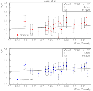
We assign the Chabrier result, to be used in the global result, to group 1 reliability.
B.1.8 Barnabe et al.
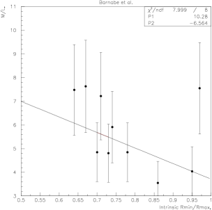
We assign the result to group 1 reliability.
B.1.9 Cardone et al. (2009)
The Cardone et al. (2009) data are described in section
9.3. (We do not use the from
the Cardone et al. (2011) data discussed in Section 9.3
since they are from Auger et al., which are already analyzed.)
The vs are shown in Fig.
58. The best fit yields:
.
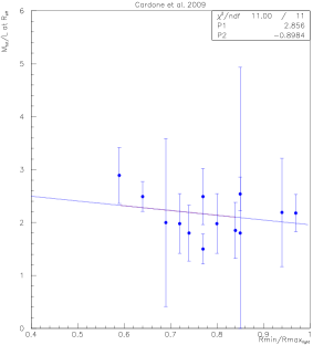
We assign the result to group 1 reliability.
B.1.10 Grillo et al.
The Grillo et al. data set is described in Section 9.8.
The vs are shown in Fig. 59
for various IMF and SMT. The best fit yields:
for results using a Salpeter IMF and a Bruzual-Charlot SMT,
for results using a Salpeter IMF and a Maraston SMT,
for results using a Chabrier IMF and a Bruzual-Charlot SMT,
for results using a Kroupa IMF and a Maraston SMT.
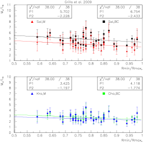
As in the main global analysis, we will used the results derived with a Chabrier IMF and a Bruzual-Charlot SMT. We assign the result to group 1 reliability.
B.1.11 Jiang and Kochanek
The Jiang and Kochanek data are described in Section 9.10.
The vs are shown in Fig. 60.
The best fit yields:
.

We assign the result to group 3 reliability.
B.1.12 Leier et al. (2011)
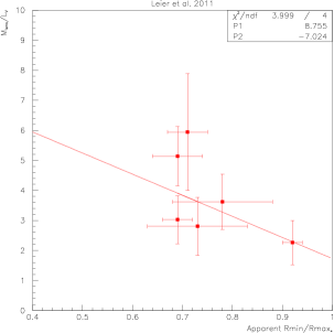
We assign the result to group 2 reliability.
B.1.13 Treu and Koopman
The data are discussed in Section 9.16. It
was found that:
, and
,
for which Fundamental Plan assumptions were made to further constrain
the data.
The results without Fundamental Plan assumptions will be used for the
global analysis. We assign the result to group 1 reliability.
B.2 Global results for
To combine the individual results, we follow the same procedure as for the main analysis (see Section 13, we choose to normalize the average to 4) and correct for projection (see Section 10.2, the same correction factor 5, determined with the total from [3]). The slopes for the individual results are shown in Fig. 62.
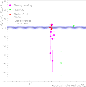
For clarity, they are plotted vs the approximate average radius value at which the are extracted. The average slope is
a value well compatible with zero. We can compare it to the results of the main analysis by normalizing the average mass over light ratios to a same value. Then, the slope for is 50 times smaller than that for .
We note that excluding the PNe/GC data sets, in case not applying the ellipticity corrections is questioned -a difference between the and analyses-, we obtain , which is still compatible with zero. Normalizing the average mass over light ratios to a same value, then the slope for is twice smaller than that for , and they are compatible within uncertainty. The inconclusive results, in the case of excluding the PNe/GC data sets, underline the limitation of this test due to its limited number of data sets and extraction methods.
Appendix C Summary table of the NGC, IC and UGC galaxies
Key: x: used. (x): used in lower reliability group. The true is indicated when available. EXC and VCXG refer to [49], see Section 7.1. XE has a similar meaning as EXG and refers to [78]. The symbol - means the galaxy is available but does not pass the selection critteria. refers to an adequate elliptical galaxy, but unused because of mismatch between the NED numbers and the ones listed in [3].
| name | Bac | Ben | Bert | Capa | Dea | Fuk | Kro | Lau | Mag01 | Mag98 | Nag | Piz | Pru | Rom | SAUR | Thomas | v.d. Mar 91 | v.d. Mar 07b | comment |
|---|---|---|---|---|---|---|---|---|---|---|---|---|---|---|---|---|---|---|---|
| 57 | x | x | |||||||||||||||||
| 83 | x | ||||||||||||||||||
| 97 | x | ||||||||||||||||||
| 194 | x | ||||||||||||||||||
| 430 | x | ||||||||||||||||||
| 547 | - | - | Arp | ||||||||||||||||
| 564 | x | ||||||||||||||||||
| 584 | x | x | x | x | |||||||||||||||
| 636 | - | - | - | - | - | - | S0? [104] | ||||||||||||
| 720 | x | x | x | x | x | x | x | CXG,XC | |||||||||||
| 741 | - | - | - | - | EXG | ||||||||||||||
| 759 | |||||||||||||||||||
| 821 | x | x | x | x | x | x | x | ||||||||||||
| 855 | x | ||||||||||||||||||
| 990 | NM | x | |||||||||||||||||
| 1008 | x | ||||||||||||||||||
| 1016 | x | x | |||||||||||||||||
| 1052 | - | 0.63 | NM | LINER/Sy2 | |||||||||||||||
| 1199 | x | x | x | ||||||||||||||||
| 1209 | - | (x) | LINER | ||||||||||||||||
| 1282 | x | ||||||||||||||||||
| 1283 | x | ||||||||||||||||||
| 1293 | x | ||||||||||||||||||
| 1344 | x | x | |||||||||||||||||
| 1374 | x | ||||||||||||||||||
| 1379 | x | - | - | - | - | spiral? | |||||||||||||
| 1395 | NM | - | - | - | _ | - | _ | CXG, XE | |||||||||||
| 1407 | NM | - | - | - | NM | _ | - | _ | EXG | ||||||||||
| 1426 | x | x | x | ||||||||||||||||
| 1439 | x | x | x | x | x | ||||||||||||||
| 1453 | (x) | (x) | LINER | ||||||||||||||||
| 1521 | x | ||||||||||||||||||
| 1549 | x | x | x | x | XC | ||||||||||||||
| 1573 | x | x | |||||||||||||||||
| 1600 | NM | - | - | - | - | - | - | EXG | |||||||||||
| 1700 | NM | - | x | - | - | - | - | - | EXG, kin. distinct core. | ||||||||||
| 2314 | NM | x | |||||||||||||||||
| 2320 | x | ||||||||||||||||||
| 2325 | x | ||||||||||||||||||
| 2340 | x | ||||||||||||||||||
| 2434 | x | x | x | x | x | CXG |
| name | Bac | Ben | Bert ola | Capa | Dea | Fuk | Kro | Lau | Mag 01 | Mag 98 | Nag | Piz | Pru | Rom | SAUR-ON4 | Thomas | v.d. Mar 91 | v.d. Mar 07b | comment |
| 2513 | x | ||||||||||||||||||
| 2663 | x | ||||||||||||||||||
| 2675 | x | ||||||||||||||||||
| 2693 | x | x | x | ||||||||||||||||
| 2694 | x | ||||||||||||||||||
| 2749 | NM | (x) | - | LINER | |||||||||||||||
| 2778 | x | x | x | x | |||||||||||||||
| 2800 | x | ||||||||||||||||||
| 2810 | x | ||||||||||||||||||
| 2865 | x | x | |||||||||||||||||
| 2954 | NM | ||||||||||||||||||
| 2974 | LINER, Sy2. | ||||||||||||||||||
| 3070 | x | x | |||||||||||||||||
| 3078 | x | ||||||||||||||||||
| 3091 | x | x | |||||||||||||||||
| 3121 | NM | ||||||||||||||||||
| 3136 | NM | ||||||||||||||||||
| 3158 | NM | x | |||||||||||||||||
| 3250 | x | ||||||||||||||||||
| 3258 | x | ||||||||||||||||||
| 3268 | (x) | LINER | |||||||||||||||||
| 3305 | x | ||||||||||||||||||
| 3309 | x | ||||||||||||||||||
| 3348 | NM | x | |||||||||||||||||
| 3377 | NM | x | x | - | x | x | 0.58 | x | VCXG | ||||||||||
| 3379 | - | x | x | - | (x) | x | - | (x) | x | - | - | LINER, VCXG 0.73 [95] | |||||||
| 3557 | NM | (x) | - | - | LINER, S0 [104] | ||||||||||||||
| 3562 | x | ||||||||||||||||||
| 3605 | NM | x | x | ||||||||||||||||
| 3608 | - | - | (x) | - | - | LINER | |||||||||||||
| 3613 | x | x | |||||||||||||||||
| 3640 | x | x | x | x | x | ||||||||||||||
| 3710 | x | ||||||||||||||||||
| 3731 | NM | ||||||||||||||||||
| 3812 | x | ||||||||||||||||||
| 3818 | x | x | x | ||||||||||||||||
| 3837 | x | x | |||||||||||||||||
| 3853 | x | x | |||||||||||||||||
| 3862 | NM | LERG | |||||||||||||||||
| 3872 | NM | x | |||||||||||||||||
| 3873 | x | ||||||||||||||||||
| 3904 | x | x | x | ||||||||||||||||
| 3923 | NM | x | x | x | x | CXG,XC | |||||||||||||
| 3940 | x | x | |||||||||||||||||
| 3962 | - | (x) | LINER | ||||||||||||||||
| 4070 | x | ||||||||||||||||||
| 4168 | x | AGN:Sy1.9 | |||||||||||||||||
| 4187 | x |
| name | Bac | Ben | Bert ola | Capa | Dea | Fuk | Kro | Lau | Mag 01 | Mag 98 | Nag | Piz | Pru | Rom | SAUR-ON4 | Thomas | v.d. Mar91 | v.d. Mar 07b | comment |
|---|---|---|---|---|---|---|---|---|---|---|---|---|---|---|---|---|---|---|---|
| 4213 | x | ||||||||||||||||||
| 4239 | x | x | |||||||||||||||||
| 4278 | - | 0.71 | x | Sy2, LINER | |||||||||||||||
| 4283 | NM | x | |||||||||||||||||
| 4365 | - | x | x | - | CXG, XC kinematically distinct core. | ||||||||||||||
| 4374 | - | x | - | x | - | AGN,LERG, LINER,Sy2,CXG | |||||||||||||
| 4387 | NM | x | - | x | |||||||||||||||
| 4406 | - | x | S0(3)/E3 | ||||||||||||||||
| 4458 | NM | x | 0.94 | x | |||||||||||||||
| 4464 | - | - | S?/Sab/S03 | ||||||||||||||||
| 4467 | NM | x | x | x | |||||||||||||||
| 4472 | - | - | - | Arp E2/S0,EXG,XE | |||||||||||||||
| 4473 | x | x | x | x | 0.50 | x | |||||||||||||
| 4478 | x | x | x | x | |||||||||||||||
| 4489 | x | x | x | ||||||||||||||||
| 4494 | - | - | - | x | x | - | x | - | - | LINER, VCXG 0.6[48] Possibly S0. Kinematically distinct core. | |||||||||
| 4510 | NM | ||||||||||||||||||
| 4551 | x | x | x | ||||||||||||||||
| 4555 | - | EXG | |||||||||||||||||
| 4564 | x | x | x | x | x | x | |||||||||||||
| 4589 | - | x | (x) | - | LINER, kinematically distinct core. | ||||||||||||||
| 4621 | NM | - | - | - | - | - | - | VCXG | |||||||||||
| 4648 | x | x | x | ||||||||||||||||
| 4649 | - | - | - | - | Arp,EXG,XE | ||||||||||||||
| 4660 | x | x | x | x | 0.71 | x | |||||||||||||
| 4673 | x | ||||||||||||||||||
| 4697 | NM | x | x | x | - | LLAGN,CXG | |||||||||||||
| 4742 | NM | x | x | x | |||||||||||||||
| 4860 | x | x | 0.80 | ||||||||||||||||
| 4864 | NM | x | |||||||||||||||||
| 4867 | x | ||||||||||||||||||
| 4869 | x | x | 0.88 | ||||||||||||||||
| 4876 | x | ||||||||||||||||||
| 4886 | NM | x | |||||||||||||||||
| 4906 | x | ||||||||||||||||||
| 4915 | x | ||||||||||||||||||
| 4926 | x | 0.87 | |||||||||||||||||
| 4946 | cD, E+(?) |
| name | Bac | Ben | Bert ola | Capa | Dea | Fuk | Kro | Lau | Mag 01 | Mag 98 | Nag | Piz | Pru | Rom | SAUR-ON4 | Thomas | v.d. Mar 91) | v.d. Mar 07b | comment |
|---|---|---|---|---|---|---|---|---|---|---|---|---|---|---|---|---|---|---|---|
| 4952 | 0.59 | ||||||||||||||||||
| 5018 | x | x | |||||||||||||||||
| 5029 | x | ||||||||||||||||||
| 5044 | - | - | (x) | EXG, XE, LINER | |||||||||||||||
| 5061 | x | ||||||||||||||||||
| 5077 | 0.50 | LINER, Seyfert1.9 | |||||||||||||||||
| 5129 | NM | x | |||||||||||||||||
| 5198 | x | x | |||||||||||||||||
| 5223 | x | ||||||||||||||||||
| 5266 | ( 0.6) | SA0 | |||||||||||||||||
| 5322 | - | - | (x) | LINER,XC | |||||||||||||||
| 5329 | x | ||||||||||||||||||
| 5490 | NM | x | x | ||||||||||||||||
| 5546 | x | ||||||||||||||||||
| 5557 | x | x | |||||||||||||||||
| 5576 | NM | x | x | ||||||||||||||||
| 5638 | NM | x | x | ||||||||||||||||
| 5642 | x | ||||||||||||||||||
| 5710 | x | ||||||||||||||||||
| 5791 | NM | x | |||||||||||||||||
| 5796 | NM | x | |||||||||||||||||
| 5812 | x | x | |||||||||||||||||
| 5813 | - | (x) | - | LINER | |||||||||||||||
| 5845 | x | x | x | 0.63 | x | ||||||||||||||
| 5846 | - | - | - | - | - | - | LINER, HII,cE,EXG,XE | ||||||||||||
| 5898 | x | ||||||||||||||||||
| 5903 | x | x | |||||||||||||||||
| 5966 | x | ||||||||||||||||||
| 5982 | - | (x) | LINER | ||||||||||||||||
| 6020 | x | ||||||||||||||||||
| 6137 | x | x | |||||||||||||||||
| 6411 | x | x | x | ||||||||||||||||
| 6487 | x | ||||||||||||||||||
| 6623 | - | - | Galaxy pair | ||||||||||||||||
| 6702 | (x) | (x) | LINER | ||||||||||||||||
| 6721 | cD, E+ | ||||||||||||||||||
| 6851 | x | ||||||||||||||||||
| 6868 | - | (x) | EXG, LINER | ||||||||||||||||
| 7052 | x | ||||||||||||||||||
| 7097 | 0.24 | (x) | LINER, counter rotating core. | ||||||||||||||||
| 7144 | x | x | x | ||||||||||||||||
| 7145 | x | x | x | x | |||||||||||||||
| 7147 | low |
| name | Bac | Ben | Bert ola | Capa | Dea | Fuk | Kro | Lau | Mag 01 | Mag 98 | Nag | Piz | Pru | Rom | SAUR-ON4 | Thomas | v.d. Mar91 | v.d. Mar 07b | comment |
| 7391 | NM | x | |||||||||||||||||
| 7454 | x | x | x | ||||||||||||||||
| 7458 | x | x | |||||||||||||||||
| 7507 | x | x | x | x | x | x | |||||||||||||
| 7618 | - | EXG | |||||||||||||||||
| 7619 | x | x | x | x | x | x | x | CXG | |||||||||||
| 7660 | x | x | |||||||||||||||||
| 7778 | x | x | |||||||||||||||||
| 7785 | x | x | x | x | |||||||||||||||
| 7796 | - | ( 0.75) | cD, E+ | ||||||||||||||||
| IC171 | - | x | E?/S0 | ||||||||||||||||
| IC179 | - | - | Likely a S0 | ||||||||||||||||
| IC948 | x | ||||||||||||||||||
| IC1152 | x | ||||||||||||||||||
| IC1211 | x | ||||||||||||||||||
| IC1459 | - | - | (x) | - | - | LINER | |||||||||||||
| IC3959 | x | ||||||||||||||||||
| IC4011 | x | ||||||||||||||||||
| IC4012 | x | ||||||||||||||||||
| IC4051 | NM | x | |||||||||||||||||
| UGC 1308 | 0.82 |
Appendix D Summary table for the SLACS lensing galaxies
x=used, (x)=used but in lower reliability group, -=available but not used (if for reasons other than standard selection, we state the reasons. No symbol=not available. Masses -from [53]- indicating that the galaxy maybe a giant are highlighted in red). Values are given without uncertainties because only the central values are used for selection. The integration range for varies from authors to authors.
| name | Ferr1 | Aug | Bar | Card09 | Card11 | J&K | Koop | Lei09 | Gril | Rotator | () | (km/s) | type/ comment |
| J0008-0004 | - | - | 912[22], [53] | 193[2] | E[1] | ||||||||
| J0029-0055 | - fit out- lier | x | x | x | 1622[22],[53] | 231[2],229[21] | E[1] | ||||||
| J0037-0942 | - | x | x | x | x | x | x | x | S[5] | 52.3 [47],4677[22], 27.3[59], 40[71][53] | 265[47],282[2],265[59] ,230[71] | E[1] | |
| J0044+0113 | x | x | x | 16596[22],[53] | 267[2] | E[1] | |||||||
| J0109+1500 | x | [53] | 251[2] | E[1] | |||||||||
| J0157+0056 | x | - lumi mism. | x | 1288[22],[53] | 295[2],295[21] | E[1] | |||||||
| J0216-0813 | - | - | - | - | - | - | - | S[5] | 7943[22],48.2[59], [53] | 334[2],333[21],332[59] | E[1] | ||
| J0252+0039 | x | x | x | x | 91[22],[53] | 170[2],164[21] | E[1] | ||||||
| J0330-0020 | x | x | - lumi mism. | x | 891[22],[53] | 220[2],212[21] | E[1] | ||||||
| J0405-0455 | x | [53] | 160[1] | E[1] | |||||||||
| J0728+3835 | x | x | x | x | 155[22],[53] | 219[2],214[21] | E[1] | ||||||
| J0737+3216 | x | - fit out- lier | x | - Fit outlier | x | x | x | 38.3 [47],8511[22], 31.2[59] ,59[71],[53] | 310[47],338[2],310[59] ,313[71] | E[1] | |||
| J0808+4703 | - | 236[2] | E[1] No Axis ratio | ||||||||||
| J0819+4534 | - | - | - | 6166[22] | 227[2],236[21] | E[1] . No Axis ratio | |||||||
| J0822+2652 | x | x | x | 3548[22],[53] | 263[2] | E[1] | |||||||
| J0903+4116 | - | - | - | 676[22], [53] | 223[2],223[21] | E[1] | |||||||
| J0912+0029 | - | - | - | - | - | - | - | - | 71.2[47],11220[22], 39[59],80[71], [53] | 313[47],322[2],326[21] ,313[59],276[71] | E/S0[1] | ||
| J0935-0003 | - (fit out- lier) | - | - | - | S[5] | 34674[22], [53] | 391[2] | E[1] | |||||
| J0936+0913 | x | x | x | 851[22],[53] | 246[2] | E[1] | |||||||
| J0946+1006 | x | x | x | 8128[22],[53] | 265[2] | E[1] | |||||||
| J0956+5100 | - | - | - | - | - | - | 66.4[47],12303[22], 37[59],67[71], [53] | 299[47],338[2], 299[59],299[71] | E[1] | ||||
| J0959+0410 | x | x | - lumi mism. | x | x | x | x | F[5] | 2692[22]7.7[59],[53] | 203[2],197[21],212[59] | E[1] | ||
| J1250+4901 | - | 256[2] | E[1] | ||||||||||
| J1250+0523 | x | x | x | x | - Fit outlier | x | x | S[5] | 1862[22],18.9[59],[53] | 252[2],252[21],254[59] | E[1] | ||
| J0959+4416 | - | [53] | 248[2] | S0[1] | |||||||||
| J1016+3859 | x | x | x | 2754[22],[53] | 254[2] | E[1] |
| name | Ferr.1 | Aug. | Bar. | Card09 | Card11 | J&K | Koop. | Leier09 | Grillo | Rotator | () | (km/s) | type/ comment |
| J1020+1122 | - | - | - | 1318[22], [53] | 290[2] | E[1] | |||||||
| J1023+4230 | x | x | x | x | 2951[22],[53] | 247[2],242[21] | E[1] | ||||||
| J1029+0420 | - | - | 215[2] | S0[1] | |||||||||
| J1100+5329 | - | - | 851[22], [53] | 187[1] | E[1] | ||||||||
| J1103+5322 | - | 196[2],196[21] | S0/SA[1] | ||||||||||
| J1106+5228 | x | x | x | [53] | 266[2] | E[1] | |||||||
| J1112+0826 | - | - | - | 10000[22], [53] | 328[2] | E[1] | |||||||
| J1134+6027 | x | x | x | 2089[22],[53] | 243[2] | E[1] | |||||||
| J1142+1001 | x | x | x | 2344[22],[53] | 225[2] | E[1] | |||||||
| J1143-0144 | x | x | x | 14125[22],[53] | 263[2] | E[1] | |||||||
| J1153+4612 | x | x | x | 2512[22],[53] | 233[2] | E[1] | |||||||
| J1204+0358 | x | x | x | x | S[5] | 4677[22],[53] | 274[2] | E[1] | |||||
| J1205+4910 | x | x | x | x | x | x | 38.6[47],5754[22], 45[71],[53] | 235[47],282[2],281[21] ,235[71] | E[1] | ||||
| J1213+6708 | - fit out- lier | x | x | 15849[22],[53] | 292[2] | E[1] | |||||||
| J1218+0830 | x | x | x | 2455[22],[53] | 218[2] | E[1] | |||||||
| J1251+0208 | - | 233[2] | S[1] | ||||||||||
| J1306+0600 | - | - | 8318[22] | 241[2] | E[1] Axis ratio not avail. | ||||||||
| J1313+4615 | - | - | 5623[22] | 266[2] | E[1] Axis ratio not avail. | ||||||||
| J1318-0313 | - | - | 2951[22] | 211[2] | E[1] Axis ratio not avail. | ||||||||
| J1330-0148 | - | - | - | - | - | - | - | 4.9[47],3.2[59],2.8[71] | 178[47],194[2], 178[59],178[71] | S0[1] | |||
| J1402+6321 | x | x | x | x | x | x | 2400[22],30.3[59],[53] | 268[2],267[21],275[59] | E[1] | ||||
| J1403+0006 | x | x | x | 1259[22],[53] | 218[2] | E[1] | |||||||
| J1416+5136 | - | - | - | 1698[22], [53] | 248[2] | E[1] | |||||||
| J1420+6019 | - | - | - | - | - | 3.9[59],[53] | 208[2],205[21],194[59] | S0[1] | |||||
| J1430+4105 | - | - | - | 7244[22], [53] | 325[2] | E[1] | |||||||
| J1436-0000 | x | x | x | 1950[22],[53] | 226[2] | E[1] | |||||||
| J1443+0304 | - | - | - | [53] | 218[2] | S0[1] | |||||||
| J1451-0239 | x | x | x | x | S[5] | 2754[22],[53] | 224[2] | E[1] | |||||
| J1525+3327 | - | - | - | 1950[22], [53] | 265[2] | E[1] | |||||||
| J1531-0105 | x | x | x | 6918[22],[53] | 280[2] | E[1] | |||||||
| J1538+5817 | x | x | x | 776[22],[53] | 194[2] | E[1] | |||||||
| J1614+4522 | - | - | 457[22] | 183[2] | E[1] Axis ratio not avail. | ||||||||
| J1621+3931 | x | x | x | 3388[22],[53] | 239[2] | E[1] | |||||||
| J1627-0053 | x | x | x | x | - Fit outlier | x | x | S[5] | 4266[22],22[59],[53] | 295[2],290[21],275[59] | E[1] | ||
| J1630+4520 | - | - | - | - | - | - | 1202[22],50.8[59], [53] | 281[2],276[21],260[59] | E[1] |
| name | Ferr1 | Aug | Bar | Card09 | Card11 | J&K | Koop | Lei09 | Gril | Rotator | () | (km/s) | type/ comment |
| J1636+4707 | - | x | x | - | x | 52.9[47],490[22], 31[71],[53] | 221[47],237[2],221[71] | E[1] | |||||
| J1644+2625 | - | 3236[22] | 229[1] | E[1] Mass axis ratio not avail. | |||||||||
| J1719+2939 | - | - | 11220[22] | 295[2] | S0[1] | ||||||||
| J2238-0754 | x | x | x | x | F[5] | 871[22],[53] | 200[2] | E[1] | |||||
| J2300+0022 | x | x | x | x | x | x | x | x | x | S[5] | 40.9[47],7079,30.4[59] ,39[71],[53] | 283[47],284[2],279[21] ,283[59],283[71] | E[1] |
| J2303+1422 | x | x | x | x | x | x | x | x | x | S[5] | 49.8[47],4571,27.5[59] ,51[71],[53] | 260[47],253[2],255[21] ,260[59],260[71] | E[1] |
| J2321-0939 | x | x | x | x | x | x | S[5] | 3388[22],11.7[59],[53] | 246[2],236[59] | E[1] | |||
| J2341+0000 | x | x | x | x | 1778[22],[53] | 206[2],207[21] | E[1] | ||||||
| J2347-0005 | - lumi mism. | 10000[22] | 404[1] | E[1] |
Appendix E Summary table for the COSMOS lensing galaxies
x=used, -=available but not used.
| name | Faure | () | (km/s) |
|---|---|---|---|
| COSMOS 0012+2015 | - No | 215[43] | |
| COSMOS 0013+2249 | - No | ||
| COSMOS 0018+3845 | x | 62[44] | 289[44],303[43] |
| COSMOS 0038+4133 | - <0, low | 14[44] | 207[44],225[43] |
| COSMOS 0047-5023 | - High | 145[44] | 383[44],313[43] |
| COSMOS 049+5128 | x | 73[44] | 313[44],380[43] |
| COSMOS 0050+4901 | - High , > | 119[44] | 386[44],342[43] |
| COSMOS 0056+1226 | - No | 337[43] | |
| COSMOS 0124+5121 | x | 36[44] | 267[44],245[43] |
| COSMOS 0211+1139 | - | 466[43] | |
| COSMOS 0216+2955 | - No | 349[43] | |
| COSMOS 0227+0451 | - No | 428[43] | |
| COSMOS 0254+1430 | - No | ||
| COSMOS 5857+5949 | - No | 398[43] | |
| COSMOS 5914+1219 | - > | 120[44] | 358[44],338[43] |
| COSMOS 5921+0638 | - (Rmin/Rmax mismatch), low | 11[44] | 189[44],221[43] |
| COSMOS 5941+3628 | x | 68[44] | 315[44],285[43] |
| COSMOS 5947+4753 | x | 86[44] | 326[44],370[43] |
| J100140+020040 | x | 30[44] | 259[44] |
| J095930+023427 | x | 29[44] | 255[44] |
Appendix F Summary table for the CL 3C295, CL 0016+16 and CL 1601+42 cluster galaxies
x=used, -=available but not used (if for a reason other than the standard selection criteria, we state the reason).
| name | van der Marel | Type |
|---|---|---|
| 3C295-834 | - shows extra structures S0 criteria: possibly S0 | E[105] |
| 3C295-968 | - S0 criteria: possibly S0 | E[105] |
| 0016-438 | x S0 criteria: unlikely to be S0 | E[105] |
| 0016-461 | - S0 criteria: possibly S0 | E[105] |
| 0016-531 | - S0 criteria: possibly S0 | E[105] |
| 0016-611 | - S0 criteria: likely to be S0 | E[105] |
| 0016-612 | x S0 criteria: unlikely to be S0 | E[105] |
| 0016-659 | x S0 criteria: unlikely to be S0 | E[105] |
| 0016-724 | x S0 criteria: unlikely to be S0 | E[105] |
| 0016-725 | - S0 criteria: possibly S0 | E[105] |
| 0016-745 | - S0 criteria: likely to be S0 | E[105] |
| 0016-2050 | - S0 criteria: likely to be S0 | E[105] |
| 1601-292 | - S0 criteria: possibly S0 | E[105] |
| 1601-524 | x S0 criteria: unlikely to be S0 | E[105] |
| 1601-619 | - S0 criteria: likely to be S0 | E[105] |
| 1601-753 | x S0 criteria: unlikely to be S0 | E[105] |
| 1601-814 | - S0 criteria: likely to be S0 | E[105] |
| 1601-2040 | x S0 criteria: unlikely to be S0 | E[105] |
| 1601-2043 | - S0 criteria: possibly S0 | E[105] |
| 1601-2060 | - S0 criteria: likely to be S0 | E[105] |
Appendix G Summary table for SL2S lensing galaxies
x=used, -=available but not used (if for a reason other than the standard selection criteria, we state the reason).
| name | Ruff | () | (km/s) | type/comment |
|---|---|---|---|---|
| J02141-0405 | - (no data) | Has a companion galaxy [50] | ||
| J02173-0513 | - | 54[88] | 257[88] | Influenced by nearby group [50] |
| J02190-0829 | x | 19[88] | 305[88] | |
| J02205-0639 | x | 28[88] | 242[88] | |
| J02251-0454 | x | 40[88] | 241[88] | |
| J02261-0420 | x | 40[88] | 266[88] | |
| J02264-0406 | - (no data) | S0? [50] | ||
| J02264-0904 | - | 65.2[88] | 301[88] | |
| J02325-0408 | x | 23[88] | 264[88] | |
| J14061-5202 | - (no data) | Influenced by nearby galaxy? [50] | ||
| J14061-5202 | - (no data) | |||
| J14113-5651 | x | 15[88] | 228[88] | |
| J22062-0057 | - (no data) | Small companion [50] | ||
| J22132-0009 | - | 22[88] | 183[88] | Edge-on disk galaxy [50] |
| J22140-1807 | - | 5.7[88] | 167[88] | Probably a S0 from mass and [50] |
| J22160-1751 | - (no data) | 282[88] | Not a true lens. [50] | |
| J221929-0017 | x | 9[88] | 263[88] |
Appendix H CDFS Summary table
x=used, (x)=used but in lower reliability group, -=available but not used, no symbol=not available. Values are given without uncertainties because only the central values are used for selection.
| Name | Rettura | van der Wel | () | (km/s) | type/comment |
|---|---|---|---|---|---|
| CDFS-1 | - | - | 20.4[86], 22.4[102] | 231[86],[102] | AGN |
| CDFS-2 | x | x | 20.0[86], 14.8[102] | 200[86],[102] | |
| CDFS-3 | x | x | 12.6[86], 12.6[102] | 300[86],[102] | |
| CDFS-4 | - (Giant) | - (Giant) | 97.7[86], 104.5[102] | 336[86],[102] | Large X-ray emm. |
| CDFS-5 | - (low ) | - (low ) | 9.8[86], 11.5[102] | 194[86],[102] | |
| CDFS-6 | x | x | 8.3[86], 5.4[102] | 208[86],[102] | |
| CDFS-7 | x | x | 15.1[86], 38.9[102] | 232[86],[102] | |
| CDFS-8 | x | x | 13.8[86], 12.0[102] | 253[86],[102] | |
| CDFS-9 | x | x | 10.0[86], 9.3[102] | 215[86],[102] | |
| CDFS-10 | - | - | 6.6[86], 6.6[102] | 275[86],[102] | O-II |
| CDFS-11 | - | - | 9.8[86], 9.5[102] | 208[86],[102] | O-II |
| CDFS-12 | x | x | 11.0[86], 9.3[102] | 262[86],[102] | |
| CDFS-13 | x | x | 14.8[86], 17.0[102] | 247[86],[102] | |
| CDFS-14 | - (low ) | - (low ) | 17.0 [86], 14.1[102] | 197[86],[102] | |
| CDFS-15 | x | x | 33.9[86], 25.1[102] | 317[86],[102] | |
| CDFS-16 | - | - | 18.2[86], 18.6[102] | 262[86],[102] | AGN |
| CDFS-17 | - | - | 58.9[86], 70.8[102] | 305[86],[102] | Spiral |
| CDFS-18 | - (Giant) | 51.3[102] | 324[102] | ||
| CDFS-19 | - | 16.6[102] | 229[102] | O-II | |
| CDFS-20 | - (low ) | - (low ) | 13.5[86], 12.6[102] | 199[86],[102] | |
| CDFS-21 | - (low ) | - (low ) | 2.6[86], 1.4[102] | 149[86],[102] | |
| CDFS-22 | - | - | 26.3[86], 28.8[102] | 225[86],[102] | AGN, Large X-ray emm. |
| CDFS-23 | - (low ) | - (low ) | 1.51[86], 1.9[102] | 70[86],[102] | |
| CDFS-24 | - | - | 63.1[86], 79.4[102] | 210[86],[102] | Spiral |
| Name | Rettura | van der Wel | () | (km/s) | type/comment |
|---|---|---|---|---|---|
| CDFS-25 | x | x | 9.1[86], 7.9[102] | 258[86],[102] | |
| CDFS-26 | - | - | 72.4[86], 67.60[102] | 249[86],[102] | Spiral |
| CDFS-27 | - (low ) | - (low ) | 10.5[86], 11.7[102] | 135[86],[102] | |
| CDFS-28 | - | - | 74.1[86], 147.9[102] | 445[86],[102] | Spiral |
| CDFS-29 | x | x | 11.7[86], 10.0[102] | 221[86],[102] | |
| CDFS-354 | - (low ) | 3.6[86] | 99[86] | ||
| CDFS-369 | - (low ) | 2.0[86] | 119[86] | ||
| CDFS-467 | - (low ) | 4.0[86] | 140[86] | ||
| CDFS-532 | x | 15.1[86] | 260[86] | ||
| CDFS-547 | - | 8.51[86] | 256[86] | E+A | |
| CDFS-571 | - | 20.0[86] | 182[86] | Sa | |
| CDFS-590 | - (low ) | 5.4[86] | 119[86] | ||
| CDFS-633 | x | 41.7[86] | 260[86] | ||
| CL1252-1 | - | - | 19.1[86], 21.9[102] | 219[86],[102] | AGN |
| CL1252-2 | x | x | 7.2[86], 8.3[102] | 216[86],[102] | |
| CL1252-3 | - | - | 21.9[86], 24.5[102] | 166[86],[102] | Spiral |
| CL1252-4 | - | - | 26.3[86], 34.7[102] | 202[86],[102] | Spiral |
| CL1252-5 | - | - | 28.2[86], 20,4[102] | 251[86],[102] | AGN |
| CL1252-6 | x | x | 9.1[86], 8.9[102] | 211[86],[102] | |
| CL1252-7 | - | - | 13.2[86], 12.9[102] | 213[86],[102] | AGN |
| CL1252-8 | - (low ) | - (low ) | 1.0[86], 1.0[102] | 63[86],[102] | |
| CL1252-9 | - (low ) | - (low ) | 1.8[86], 2.2[102] | 102[86],[102] | |
| CL1252-6106 | x | 30.2[86] | 294[86] | ||
| CL1252-9077 | - (low ) | 7.9[86] | 130[86] | ||
| CL1252-4419 | - (Giant) | 141.3[86] | 302[86] | Interacting | |
| CL1252-4420 | - (Giant) | 97.7[86] | 232[86] | Interacting |
Appendix I Cluster CL1358+62 elliptical galaxies summary table
x=used -=available but not used.
| ID | Kelson | type/comment |
|---|---|---|
| 212 | x | |
| 242 | - | |
| 256 | - | |
| 303 | - | |
| 360 | x | |
| 375 | - | |
| 409 | x | |
| 412 | x | |
| 531 | - | |
| 534 | x | |
| 536 | - |
Appendix J Summary table for other lensing galaxies
x=used, (x)=used but in lower reliability group, -=available but not used (if for a reason other than standard selection criteria, we stated the reason), no symbol=not available. Values are given without uncertainties because the central values only are used for selection. The integration value for varies from authors to authors.
| Name | Kee | Jack | J&K | Lei 09 | Lei 11 | Fer 05 | Treu 04 | () | (km/s) | type/comment |
|---|---|---|---|---|---|---|---|---|---|---|
| 0047-28108 | - | x | x | x | x | 58[59] 21[71], 33[72], 34[46], 41[98] | 250[59], 229[71], 254[103] | |||
| Q0142-100 | x | x | x | 46[72], 25[46] | 224[103] | E[60] | ||||
| B0218+357 | - | - | 2[58] | S[60],[70],[58] | ||||||
| CFRS-3.1077 | - (no data) | |||||||||
| C0302+006 | - | x | 67[59], 67[98] | 256[59], 251[98] | Part of small group?[98] | |||||
| MG0414+0534 | - (no z values) | x | x | x | 103[72], 83[46], 24[58] | 303[103] | E[60] | |||
| B0712+472 | - | x | - | 16[72], 9[58] | 181[103] | E[60] | ||||
| MG0751+2716 | - (intera cting) | E[60] | ||||||||
| HST0818 | - ( interac.? No axis ratio) | - ( interac.? No axis ratio) | 37[72], 67[46] | 251[103] | ||||||
| RXJ0911 | - (not true lens?) | 73[72] | 260[103] | |||||||
| FB0951+263 | - | 5[46] | 128[103] | (probably S0 from mass and ) | ||||||
| BRI0952-0115 | - (no z values) | - | - | 15[72], 5[46] | 117[103] | E[60] (probably S0 from mass and ) | ||||
| Q0957+561 | - (intera cting) | - (intera cting) | - (intera cting) | 305[71], 151[72] | 431[103], 288[71] | E[60] | ||||
| LBQS1009 | x | - | 65[72], 18[46] | 198[103] | ||||||
| Q1017-207 | - | 5[46] | 151[103] | (probably S0 from mass and ) | ||||||
| FSC10214+4724 | 241[103] | |||||||||
| B1030+071 | - | - (intera cting) | - | 55[72], 16[46], 22[58] | 218[103] | |||||
| HE1104-1085 | x | - | 73[72], 122[46] | 316[103] | E | |||||
| PG1115+080 | - | - | - | - | - | 17[59], 8.2[71], 17[72], 28[46] | 210[103], 281[59], 191[71] | E[60],peculiar? [59],interacting |
| Name | Kee | Jack | J&K | Lei 09 | Lei 11 | Fer 05 | Treu 04 | () | (km/s) | type/comment |
|---|---|---|---|---|---|---|---|---|---|---|
| B1127+385 G1 | - | 2.7[58] | Late type? [64] | |||||||
| B1127+385 G2 | - | 1.1[58] | Late type? [64] | |||||||
| MG1131+0456 | - (intera cting) | |||||||||
| B1152 | - (intera cting) | 30[72] | ||||||||
| HST12531-2914 | - (no z values) | NA | E | |||||||
| HST14113+ 5211 | - | 34[46] | 190[103] | |||||||
| HST14176+ 5226 | x | - | x | - | x | 71[59],34.3[71], 118[46],71[98] | 292[103],212[59], 245,224[98] | E[60] | ||
| B1422+231 | - (intera cting) | - | - (intera cting) | 5.7[72], 16[46], 12[58] | 160[103] | E[60] (probably S0 from mass and ) | ||||
| SBS1520 | x | x | 42[72], 27[46] | 220[103] | ||||||
| H1543-535 | - | - (no data) | - | 3.4[59], 3.4[98] | 108[59], 116[98] | (probably S0 from mass and ) | ||||
| COMBO15422 | 63[77] | 305[77] | S0-like [77] | |||||||
| MG1549+3047 | - | - ( disk? fit outlier) | 12[59] | 188[103], 227[59] | E[60] | |||||
| B1600+434 | - (poor under) | - | - (intera cting) | 16[72], 12[58] | E, maybe S[60] S[58] | |||||
| B1608+656 | - | - | - | - | - | 28[103],42[72], 85[46],52[58] | 292[103], 247[72] | E, maybe S[60], may have a companion | ||
| MG1654+1346 | x | 206[103] | E, maybe S[60] | |||||||
| PKS1830-211 | S[70] | |||||||||
| B1933+503 | - | - | S [96] | |||||||
| B1938+666 | x | 6[58] | E ? [62] | |||||||
| MG2016+112 | - | x | - | - | 110[59], 20.41[71], 52[72], 110[98] | 304[59], 304[71], 299[103] | Giant E [72] | |||
| B2045 | - | - (intera cting?) | 173[72] 86[58] | 378[103] | Maybe Sa | |||||
| B2114+022 G1 | - | 26 [58] | Post starburst elliptical. E+A. Dust makes unreliable [26] | |||||||
| B2114+022 G2 | x | 52 [58] | E [26] |
Appendix K Summary of the individual analyses
In the table below, we summarize the results of each individual analysis described from Section 4 to Section 9. Col(1): publication reference. Col(2): method used to compute the dark content. Col(3): best fit result (not yet normalized to =). Col(4) : number of elliptical galaxies that passed the selection criteria of Section 3.1. Col(5): reliability group, see Section 13, Col(6): weight factor wf, see Section 13. This a multiplicative factor to the uncertainties: the higher wf, the less impact the data set has on the global average. Col(7): specific notes regarding the analysis. Here, we give the best fit result in function of ellipticity rather than . “-” means that the data was not used in the global average.
| Ref. | Method | Best fit | stat | rg | wf | Notes |
|---|---|---|---|---|---|---|
| [3] | Virial | 64 | 2 | 1.50 | Added requirement that the galaxy characteristics listed in the 1985 Ref. [3] are compatible with recent characteristics given in NED [110]. Results using ellipticity corrections from isotropic method. | |
| [3] | Virial | 11 | 2 | 1.13 | Same additional selection criterion as above. Results using ellipticity correction from isotropic method. | |
| [3] | Virial | 11 | 1 | 1.13 | Same additional selection criterion as above. Results using ellipticity correction from anisotropic method. | |
| [6] | Virial | 35 | 3 | 2.37 | ||
| [61] | Virial | 5 | 4 | 1.00 | Distant galaxies (cluster CL1358+62). Added selection criterion to minimize contamination from boxy galaxies. | |
| [69] | Virial | 10 | 4 | 6.09 | extracted for galactic cores. Same added selection criterion as [3]. | |
| [71] | Virial | 8 | 2 | 1.00 | Distant galaxies strongly lensing. Also analyzed with strong lensing method. | |
| [84] | Virial | 102 | 2 | 1.32 | ||
| [86] | Virial | 16 | 3 | 1.35 | Distant galaxies. obtained with composite stellar population models using a Kroupa IMF [68]. | |
| [102] | Virial | 13 | 3 | 1.35 | Distant galaxies. | |
| [17] | Modeling | 6 6 | 1 1 | 1.38 1.38 | Two estimates of provided. One based on a 2-integral Jeans model and one on a 3-integral Schwartzchild model [92]. | |
| cap. 2013a | Modeling | 31 | 1 | 1.86 | ||
| cap. 2013b | Modeling | 31 | 1 | 1.86 | ||
| [67] | Modeling | 10 10 | 1 1 | 1.17 1.17 | Kept LINERS, AGN and Seyfert galaxies because isothermal or virial equilibrium is not required. | |
| [73] | Modeling | 7 | 1 | 1.33 | ||
| [97] and [108] | Modeling | 7 7 | 1 2 | 1.16 1.63 | Distant galaxies (Coma cluster and Abell 262 cluster). [97] was assumed to be independent of radius. | |
| [104] | Modeling | ) | 9 | 1 | 1.47 | |
| [105] | Modeling | 19 | 2 | 1.00 | Distant galaxies. | |
| [106] | Modeling | 17 | 1 | 2.04 | Homogenized compilation of literature (local galaxies). | |
| [16] | PNe/GC | 5 | 2.14 | Relaxed selection: includes all galaxies except the disrupted ones, the ones showing possible interactions and the ones clearly non-elliptical. |
| Ref. | Method | Best fit | stat | rg | wf | Notes |
|---|---|---|---|---|---|---|
| [30] | PNe/GC | 7 | 1 | 1.24 | Relaxed selection. | |
| [74] | PNe/GC | 8 | 1 | 1.14 | ||
| [87] | PNe/GC | 3 | 1 | 1.22 | True axis ratios are from [17] , [48] and [95]. | |
| [49] | X-ray | 7 | 2 | 1.17 | ||
| [78] | X-ray | 3 3 2 | 2 2 2 | 1.17 1.17 1.17 | ||
| [9] and [8] | Gas disk | 4 | 1 | 1.15 | Relaxed selection (kept LINERS and/or Sy types) and are the radii of the elliptical galaxy triaxial shape model. | |
| [83] | Gas disk | 4 | 1 | 1.15 | Relaxed selection (kept LINERS and/or Sy types) and are the intrinsic axis ratios of the triaxial galaxy. | |
| [2] | Lensing | 34 34 34 34 | 1 1 1 1 | - - 2.04 - | S0 galaxies are already identified in [83]. Thus standard km.s-1 criterion is not applied in this analysis (and all other analyses using SLACS data). Mass ratios extracted using either a Chabrier [25] or a Salpeter IMF [89]. | |
| [5] | Lensing | 10 10 | 1 1 | 2.05 - | formed with DMf using either a Chabrier [25] or a Salpeter IMF [89]. | |
| [21] | Lensing | 13 13 | 1 1 | - 5.12 | ||
| [22] | Lensing | 36 36 36 36 | 2 2 2 2 | - 4.92 - 1.00 | Use Secondary Infall Model and Salpeter IMF. | |
| [44] | Lensing | 7 | 1 | 1.00 | ||
| [46] | Lensing | 4 4 | 1 1 | 1.29 - | determined with a Chabrier or a Salpeter IMF. | |
| [47] | Lensing | and | 4 4 | 1 1 | 1.80 - | |
| [53] | Lensing | 40 40 40 40 | 1 1 1 1 | - - - 2.00 | Stellar Composite Model used to obtain with two different sets of metallicity template (Bruzual & Charlot [14] or Maraston [75]) and three different IMF (Salpeter [89], Kroupa [68] or Chabrier [25]). | |
| [58] | Lensing | 4 | 3 | 1.37 | ||
| [59] | Lensing | 12 12 | 2 2 | 6.24 - | Use results with adiabatic compression (favored by the authors’ analysis). | |
| [60] | Lensing | 3 3 | 3 3 | - | Due to the small number of galaxies, we relaxed the S0 rejection criterion and used km.s-1. Thus, this result is weighted out in the global average. | |
| [65] | Lensing | 9 9 | 1 1 | 2.52 - | ||
| [71] | Lensing | 8 | 1 | 4.98 | ||
| [72] | Lensing | 3 | 2 | 2.83 | ||
| [88] | Lensing | 7 7 7 7 7 7 | 2 2 2 2 2 2 | 1.00 - - - 1.00 - | The determined with a Chabrier or a Salpeter IMF are for at . at does not need IMF input. | |
| [98] | Lensing | 3 | 1 | 1.23 |
Appendix L Detailed analysis of the Bacon et al. data
This section provides the details of the analysis done using the Bacon et al. data. The results reported here are slightly different from the results given in Section 4.1 Since additional corrections, mostly addressing possible correlations, are applied. In addition, some of the NED data used may have become obsolete as they are from the 2008 database. The purpose of this section is to define the analysis method, identification requirement and most importantly, correlation investigations. The slight difference with Section 4.1 is thus irrelevant.
L.1 Data quality and galaxy selection
We apply our usual selection criteria. In addition, we reject the 8 last galaxies of [3] for lack of reference. Since the data [3] are old, we verified that they agree with data also available from NED (as of 2008). We exclude121212We exclude the data rather than correct, with the NED value, and other quantities: we prefer to assume that the discrepancy reflects a difficult measurement and hence a suspicious datum, rather than assuming that NED is correct and Ref. [3] wrong. from our sample galaxies for which their distance to Earth (redshift based) disagree by more than 20% between NED and [3]. We apply the same criterion for the apparent axis ratio . The apparent magnitude from NED and [3] always agree within 10%, so no galaxy is excluded on the basis of an apparent magnitude discrepancy. We note that some of the uncertainties quoted in [3] may be underestimated since some of the sets are incompatible (assuming that the NED data are more accurate). Comparing the analysis done using the galactic characteristics from [3] and the analysis done using that of NED is useful for studying if the correlations seen between the galactic characteristics are due to measurement bias rather than a physical relation or an observational bias. When no uncertainty was available from NED, we used the uncertainty reported in [3]. To check for possible biases, we fit the Ref. [3] vs NED data for , distance moduli , and apparent magnitudes using a linear function, see Figs. 63, 64, 65 and 66.131313We will account here for the horizontal uncertainty in a recursive way: we first fit the distribution without accounting for the horizontal error bars. We then use this first fit result to transform the horizontal errors in vertical ones and add the sum in quadrature. This procedure assumes that all errors are gaussian. No significant biases are found, except for the non-redshift based . Using the NED data, particularly its non-redshift based , significantly strengthen the vs correlation.
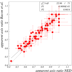
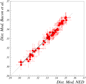
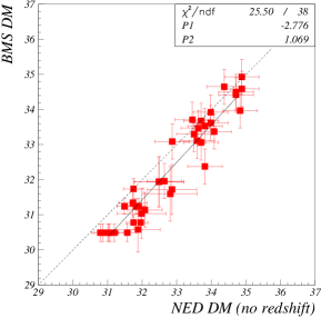

All in all, we kept 73 galaxies in the sample. The list is: NGC57, 83, 97, 430, 584, 636, 720, 741, 990, 1008, 1016, 1199, 1209, 1426, 1439, 1521, 1573, 2675, 2693, 2778, 2800, 2810, 2954, 3070, 3562, 3640, 3710, 3812, 3818, 3837, 3853, 3904, 3940, 4070, 4187, 4213, 4239, 4365, 4473, 4478, 4489, 4510, 4551, 4564, 4648, 4660, 4860, 4869, 5029, 5223, 5329, 5546, 5642, 5710, 5845, 5966, 6020, 6137, 6411, 6487, 6623, 7391, 7454, 7458, 7507, 7619, 7660, 7778, 7785, and IC179, 948, 1152 and 1211. Among this sample, 12 galaxies have available using two additional virial formulae presumably less sensitive to unknown true flattening [3]. They are: NGC584, 720, 2778, 3818, 3904, 4365, 4473, 4478, 4551, 5845, 7619 and 7785.
L.2 Data analysis
Selection is applied to the data sample. In addition, the ratio redshift distance from NED over distance from [3] is applied to to correct these ratios on a galaxy per galaxy basis. We use from [3] for consistency with the calculations, as it is an important ingredient of the calculation. The results for the three are shown in Figs. 67, 71 and 72.
Correcting with the NED distance is not significant: not correcting yields similar results (Fig. 68). Similarly, using NED’s does not change significantly the results (Fig. 69). All the fits give a slope of .
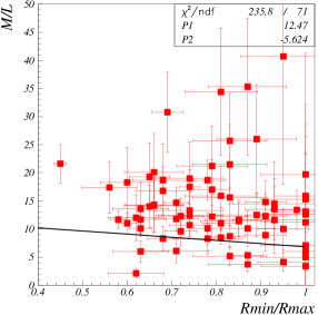
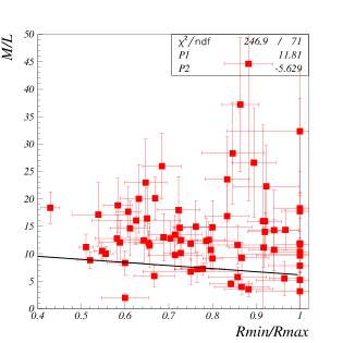
The best linear fit for the data in Fig. 67 is . A non-zero slope indicates a correlation, so the fit yields a significantly negative slope with a sigma confidence141414The point at stands outside the distribution. Although there is no reason to remove it since it passes the selection criteria, we checked that this datum is not solely responsible for the observed correlation. After removing the datum, the best fit slope becomes , a 1.7 sigma effect. Anticipating upcoming corrections, the final result (Fig. 95) becomes after removing the datum, that is a 4.7 sigma effect., but with a of 3.4. A order polynomial yields a similar . As we will show, the large of the linear fit comes mostly from the effect of the projection of the 3D elliptical galaxy shapes into flat ellipses on the observation plane. This transforms a, e.g., linear dependence with apparent axis ratio into a non-linear dependence with the real axis ratio.
Alternatively, to assess the correlation, one can compute the Pearson correlation coefficient given by the covariance of and divided by their standard deviations: . We have and larger values of indicates clearer (small dispertion) and/or stronger (steeper slope) correlations. However, since such statistical analysis does not account for statistical weights, contrarily to a fit, it is ill-suited for our sample that displays a large range in uncertainties. This problem can be partly circumvented by keeping data of a given absolute precision, see Fig. 70.
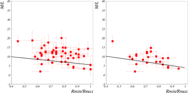
Keeping data for which the uncertainty on is smaller than 5 yields (the sample is reduced to 48 galaxies. For this sample, the best linear fit is , to be compared to the results in Fig. 67). Applying a tighter selection reduces the sample to 23 galaxies and yields (the best linear fit is ). Such values of reveal a medium to large correlation between and the axis ratio and confirm the conclusion from the fit method. Interestingly, selecting the highest precision data strengthen the vs correlation, both for the determination using of the Pearson criterion and for the determination from the linear fit.
Results using the two other determinations of that employ an additional observable (maximum stellar rotation velocity) confirm in both cases (Figs. 71 and 72) the significant negative slope, with similar .
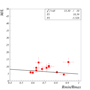
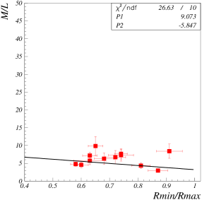
Although we assume in this appendix that the correct distances are given by the redshifts, we show in Fig. 73 the result using NED distances not based on redshifts. The vertical scale changes following (distance without redshift)/(distance from redshift). In that case, since the no-redshift distances are systematically larger than the distances estimated from redshifts (see Fig. 65), the correlation is even stronger, with a slope of i.e, a 5 effect. (We note that the 40 galaxies that have no-redshift distances available already had a larger correlation, even before the distance correction is applied to .) The Pearson coefficient, after removing data with uncertainty of greater than 5 (this reduces the sample to 25 galaxies), is .
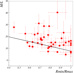
L.3 Correlations
Studying correlations is critical since they can bias the studied correlation. Possible measurement or observation biases not directly related to and can propagate to them via correlations. Furthermore, a (not understood) correlation can be removed either by sample selection or be mathematically corrected for. However, this must be done carefully: if this correlation is actually a consequence of a dependence with propagating via other correlations, correcting or selecting it could wrongly suppresses the correlation. Thus, it is important to check the correlations between variables characterizing an elliptical galaxy and make sure they do not originate from measurement or observation biases. It should then be checked what is the effect of these correlation on vs .
Except in one occasion, we do not investigate the possibility that characteristics other than the ones given in [3] are correlated to both and . This could certainly occur and it is a limitation of our analysis to keep in mind. (The exception mentionned above is the metallicity content of elliptical galaxies, see Section L.3.2.)

L.3.1 Expected correlations
-
•
Effective radius (Kpc) vs velocity dispersion ; effective radius (Kpc) vs absolute blue magnitude ; central velocity dispersion vs absolute blue magnitude : those are the empirical fundamental plane relations [11], respectively the third fundamental plane relation; the Kormendy relation [66] and the Faber-Jackson relation [41].
-
•
Distance Moduli vs effective radius and integrated blue magnitude : they are trivial reductions of the apparent intensities of quantities with their distance to the observer151515If the span is large, i.e, we observe galaxies over a large time span over which they have time to evolve, we would also expect a correlation between and the galaxy characteristics, e.g. the absolute blue magnitude , effective radius , axis ratio or velocity dispersion . Decrease of galaxy magnitudes () with time is established. Structure evolution with time () has been observed by comparing high redshift galaxies to local ones [45]: older massive elliptical galaxies are more compact than younger ones. This would imply a -dependence of the axis ratio as well since the decrease of the galaxy size with time increases the rotation speed. Finally, it is known that relaxation with time reduces the central velocity dispersion. However, in our sample, varies between and ., which corresponds to distances of 33 Megalight-years (Mly) and 411 Mly. The time span considered is thus 378 Myears. Since the galaxies were formed long before 411 Myears ago, and since we removed from our sample galaxies displaying signs of mergers or disturbances, galaxies had time to relax to their equilibrium. Consequently, we do not expect the sample galaxies to evolve significantly during the relatively short 378 Myears time span..
-
•
Apparent blue magnitude vs apparent radius : the larger the apparent radius is, the higher the apparent magnitude tends to be.
-
•
Surface Brightness vs absolute magnitude . Central surface brightness vs absolute blue magnitude correlation has been observed [10].
-
•
Integrated blue magnitude vs surface brightness : these two quantities describing the luminosity of a galaxy are related by the equation given in Fig. 74, where is in arcsec.
-
•
Axis ratio vs effective radius : this reflects the galaxy structure, with small galaxies tending to be more elongated.
-
•
Mass to light ratio vs effective radius : at both ends of the mass spectrum, dwarf and giant (e.g. BrClg) galaxies tend to have higher . However, those are excluded from our sample. Consequently, we do not expect a strong correlation here.
-
•
Mass to light ratio vs velocity dispersion . The virial theorem links potential and kinetic energy.
L.3.2 Correlation study
In this section we used arrow symbols with the following meanings:
-
•
: strong correlation;
-
•
: clear correlation;
-
•
: clear but weaker correlation;
-
•
: unclear correlation. Weak if it exists.
The correlation strengths are summarized in Figs. 88 (summary table), 89 (clear correlations) and 90 (unclear weak correlations).
Correlations with apparent from [3]
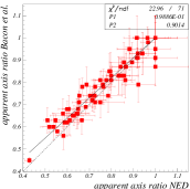
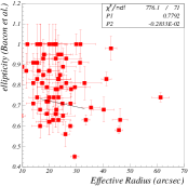
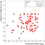
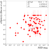
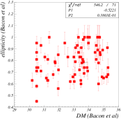
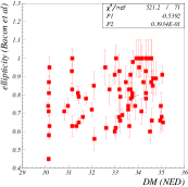
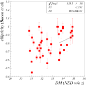
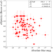
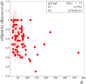
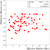
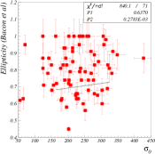
The origins of the correlations are, from the top left plot to the bottom right one:
- 1.
-
2.
Apparent axis ratio from [3] vs apparent effective radius : this possible weak correlation may be a measurement/observation bias. The more recent data from NED display a similar, even slightly stronger correlation. It could be a consequence of the correlations. Using the fit results161616This type of calculation is merely indicative, given the large of the fits. and yields , in agreement with the observed . Since is a measurement bias, is an indirect measurement bias.
-
3.
Apparent axis ratio from [3] vs integrated blue magnitude : this weak correlation may be a measurement/observation bias. The more recent data from NED, in particular the NED apparent axis ratio vs magnitude from NED in Fig. 76, display similar correlations. This correlation could be a consequence of the correlations. Using the fit results and yields , in agreement with the observed . Thus, is an indirect measurement bias.
-
4.
Apparent axis ratio from [3] vs magnitude from NED: same as above.
-
5.
Apparent axis ratio from [3] vs from [3]: this weak correlation could be a measurement bias: the further the galaxy, the harder it is to observe and so the rounder it tends to appear due to resolution. The more recent data from NED, in particular the NED apparent axis ratio vs magnitude from NED in Fig. 76, displays a somewhat smaller correlations, supporting that it is a measurement bias.
-
6.
Apparent axis ratio from [3] vs from NED using redshift information: see above.
-
7.
Apparent axis ratio from [3] vs from NED without redshift information: see above.
-
8.
Apparent axis ratio from [3] vs absolute blue magnitude: the possible weak correlation could come from a measurement bias (the result from NED in Fig. 76 has somewhat smaller correlations). However, it seems to be a consequence of the and correlations: using the fit results and yields . Using the fit results and yields . Adding both results yields , in reasonable agreement with the observed , suggesting that the correlation is an indirect measurement bias. Alternatively, we note that a correlation between axis ratio and mass is known: heavier (hence more luminous) galaxies tend to be rounder. Although we have rejected the heaviest elliptical galaxies, we may be seing here the same correlation.
-
9.
Apparent axis ratio from [3] vs surface brightness : this clear correlation cannot be a (direct) measurement bias: it does not have the expected pattern (the dimer, the more difficult the measurement so the larger would be). In addition, the newer NED data indicate a stronger correlation, see Fig. 76. This correlation could be a consequence of the correlations. Using the fit results and yields , in agreement with the observed . This supports that the correlation is an indirect measurement bias.
-
10.
Apparent axis ratio from [3] vs effective radius (parsec): this possible correlation would agree with the observation that smaller galaxies tend to be more elongated. However, this correlation appears to be a consequence of the correlations. Using the fit results and yields , in agreement with the observed . This is an indirect measurement bias.
-
11.
Apparent axis ratio from [3] vs velocity distribution . No significant correlation is seen. The newer data from NED show no correlation. We expected that , , and , would contribute to secondary correlations: using the fit results and yields . Using the fit results and yields . Using the fit results and yields . Using the fit results and yields . Naively adding linearly the four results yields , a 2 sigma disagreement with the observed . However, these results cannot be simply added linearly because of the strong correlation between & . Also, & , & and & show significant correlations. We assume that overall the four results mostly cancel each other as suggested by the opposite signs of the correlations.
Correlation with apparent from NED
The origins of the correlations are discussed in the previous section (Section L.3.2).
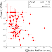
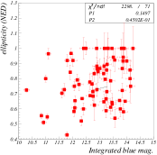
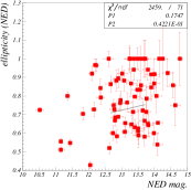
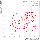
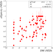
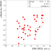
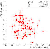
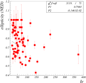
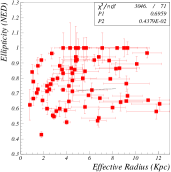
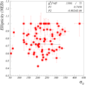
Apparent effective radius correlations
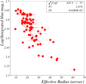
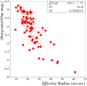
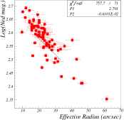
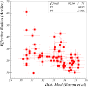
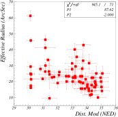
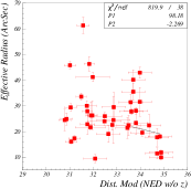
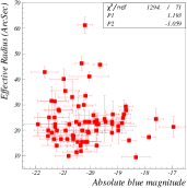
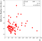
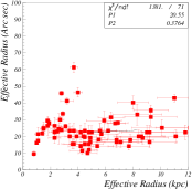
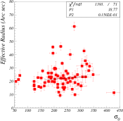
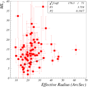
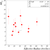
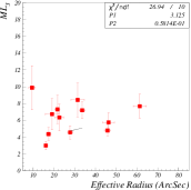
The origins of the correlations are, from the top left plot to the bottom right one:
-
1.
Effective radius vs integrated blue magnitude : this strong correlation is expected from physics since the larger the apparent radius, the larger the apparent magnitude tends to be.
-
2.
Same as above but with a linear vertical scale.
-
3.
vs magnitude from NED: same as above.
-
4.
vs from [3]: this is the trivial decrease of apparent size with distance to the observer.
-
5.
vs from NED using redshift information: same as above.
-
6.
vs from NED without redshift information: same as above.
-
7.
vs absolute blue magnitude: no clear correlation is seen. A linear (or any functional) fit fails to account for the data distribution. We were expecting a clear secondary correlation of opposite sign from the correlations. Using the fit results and yields . The other important contribution is from the correlations. Using the fit results and yields . Again, these two results cannot be added linearly because of correlations between & , but the opposite signs of the two correlations suggest a cancellation.
-
8.
vs surface brightness : a weak possible correlation is seen. The correlations and can both contribute to create it. Using the linear fit results and yields . Using the linear fit results and yields . As & are strongly correlated, we cannot simply add these results, but their same sign suggests a strong correlation, in disagreement with the sign of the observed possible correlation. However, this disagreement may stem from the unreliable fit. The correlation itself, if it exists, is weak.
-
9.
vs effective radius (parsec): because a distance in Kpc is given by , then ( converts rad in arcsec).
-
10.
vs velocity distribution : no, or unclear, weak correlation.
-
11.
vs : this weak correlation may arise from the correlations , , and . Using the linear fit results and yields . Using the linear fit results and yields . Using the linear fit results and yields . Using the linear fit results and yields . & , & , & and & are correlated. However, adding the contributions, we obtain , just 2.3 away from the observed . This suggests that this weak correlation may originate from the four correlations , , and .
Integrated blue magnitude correlations
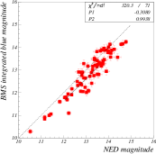
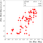
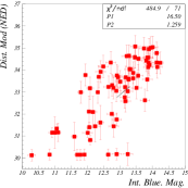
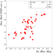
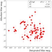
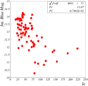
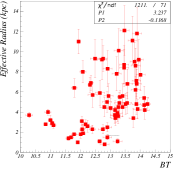
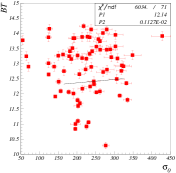
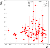
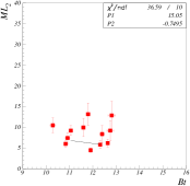
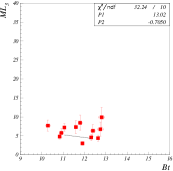
The origins of the correlations are, from the top left plot to the bottom right one:
-
1.
Integrated blue magnitude vs magnitude from NED: this was already discussed (see Fig. 66).
-
2.
vs from [3]: this clear strong correlation is due to the trivial decrease of apparent brightness with distance to the observer.
-
3.
vs from NED using redshift information: same as above.
-
4.
vs from NED without redshift information: same as above.
-
5.
vs absolute blue magnitude: no or little correlation is observed. However we expect 3 strong secondary correlations to contribute: , and . Using the linear fit results and yields . Using the linear fit results and yields a contribution . Using the linear fit results and yields a contribution . These contributions cannot be linearly added since & , &, & and & display significant correlations.
-
6.
vs surface brightness : these observables are related by .
-
7.
vs effective radius (parsec): we expect a positive correlation from . This is observed. However, we cannot verify it numerically due to the failure of the vs fit.
-
8.
vs velocity distribution : no correlation is seen. We expected some contribution from , and . Using the linear fit results and yields a contribution . The second correlation cannot be computed due to the failure of the vs fit. However, we can estimate that it yields a contribution . Overall, the two small contributions agree with the observed absence of correlation (the smaller is unreliable due to the large of the fit).
-
9.
vs . No correlation is expected (all secondary correlations involve a weak/unclear correlation). This is what is observed.
Magnitude from NED correlations
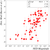
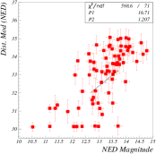
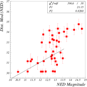
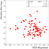
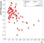
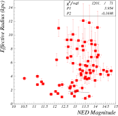
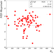
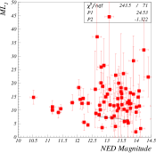
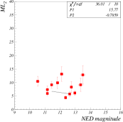
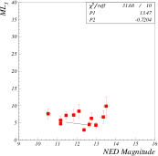
The origins of the correlations are similar to the ones discussed in Section L.3.2.
Distance Moduli ([3]) correlations
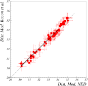

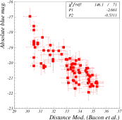
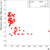
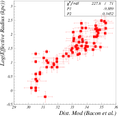
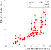
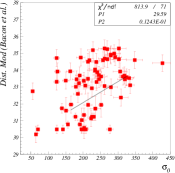
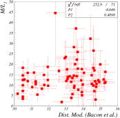
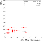
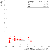
The origins of the correlations are, from the top left plot to the bottom right one:
- 1.
- 2.
-
3.
from [3] vs absolute blue magnitude: we observe a strong correlation. Since we do not expect significant time evolution, this must be an observational bias: at large , more luminous galaxies are easier to observe. At smaller , both luminous and dimmer galaxies can be seen, but the presence probability of luminous elliptical galaxies is smaller since the corresponding volume is smaller and luminous galaxies are rarer than dimmer ones. In all, luminous galaxies tend to be seen at large distances while dimmer ones are seen at shorter distances. That this is a measurement bias and not a physical characteristic is confirmed by the absence of vs correlation, see point 8. below.
-
4.
from [3] vs surface brightness : surface brightness is independent of distances. The correlation seen is expected from the fact that and are almost linearly related (see the two next plots) and that and are also correlated (consequence of the Kormendy relation [66]). Indeed, the pattern of vs strongly resembles the one of of vs . This is an indirect consequence of the observation bias.
-
5.
from [3] vs effective radius (parsec): a significant secondary (indirect) correlation is expected from the Kormendy correlation and correlation. Using the linear fit results and yields . Another indirect correlation is expected from the fundamental plan correlation and the correlation. Using the fit results and yields . These secondary correlations are similar to the observed (linear fit). In addition, we expect the same type of observational bias as for the vs correlation. All in all, this is a consequence of the observation bias.
-
6.
Same as above but with a linear vertical scale.
-
7.
from [3] vs velocity distribution : we observe a significant correction of with . We expect strong secondary correlations due to theKormendy relation, the vs observational bias, the Faber-Jackson and the fundamental plane relations. This is again an indirect consequence of the and observation biases.
-
8.
from [3] vs : we observe little correlation. This confirms that the vs absolute blue magnitude correlation is an unphysical bias: if the blue magnitude truly depended on , then, the would display a similar dependence since we do not expect the mass of an undisturbed galaxy to evolve with time.
Distance Moduli (NED with redshift information) correlations
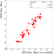
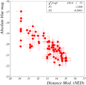
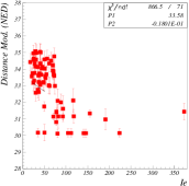
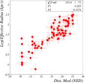
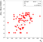
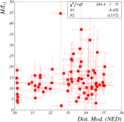
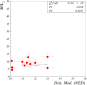
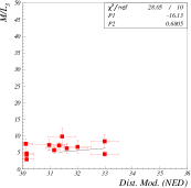
The origins of the correlations are the same as the ones discussed in Section L.3.2.
Distance Moduli (NED without redshift information) correlations
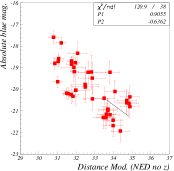
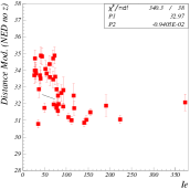
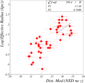
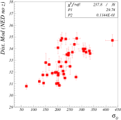
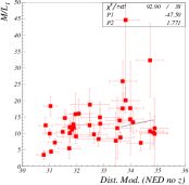
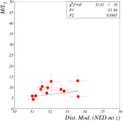
The origins of the correlations are the same as the ones discussed in Section L.3.2.
Absolute magnitude correlations
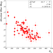
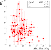
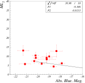
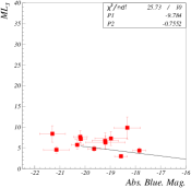
The origins of the correlations are, from top left to bottom right:
-
1.
Absolute blue magnitude vs surface brightness : this pattern agrees with the observed central surface brightness vs relation [10]. However, it could also arise from two secondary correlations: and possibly . Using the linear fit results and yields . Using the linear fit results and yields a negligible contribution . This agrees with the observed . This plot, however, suggests to reject the two lowest points since they are close to the dwarf elliptical locus [10].
-
2.
vs effective radius (parsec): this is the well known Kormendy relation [66].
-
3.
vs velocity distribution : this is the well known Faber-Jackson relation [41].
-
4.
vs : a clear weak correlation is seen. It seems to be due to the virial theorem and the Kormendy relation: . Using the linear fit results and yields . This is in qualitative agreement with the observed correlation. The value from the fit: is underestimated since a linear form is not adapted for the fit. Another contribution could result from the fact that luminous/large elliptical galaxies tend to have stars that are more metal-rich than less luminous elliptical galaxies [94]. This tends to increase the with increasing absolute luminosity . In principle, this possibility has to be ruled out in order to cleanly interpret a dependence of with . In practice, there is only an uncertain weak correlation between and so it would have little influence on the vs dependence. Furthermore, as explained in the Section L.1, the most luminous galaxies are excluded from our data set. All in all, we can ignore the consequence that large elliptical galaxies are more metal rich.
Surface Brightness correlations.
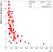
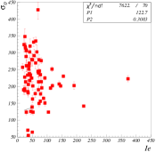
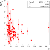
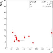
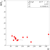
The origins of the correlations are, from top left to bottom right:
-
1.
Surface brightness vs effective radius (parsec): this is expected from the Kormendy relation: it implies that the larger the galaxy, the lower its surface brightness (see e.g. [11] page 24), as seen on the plot.
-
2.
vs velocity distribution : this is expected from the distributions.
-
3.
vs : this is similar to the just discussed vs distribution due to the strong correlation.
Absolute effective radius correlations
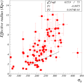
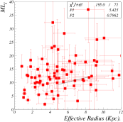
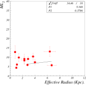
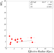
The origins of the correlations are, from left to right:
-
1.
Effective radius (parsec) vs velocity distribution : this correlation is the well known plane relation.
-
2.
Effective radius (parsec) vs : there is no or little correlation. This is opposite to what would have been expected if our sample had included dwarf elliptical galaxies, since they tend to have larger . This validates our choice of selection critteria.
Central velocity distribution correlations
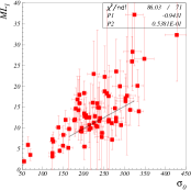
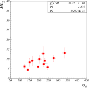
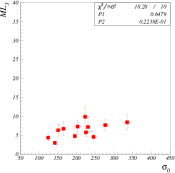
The origin of the velocity distribution vs ratios correlation is the virial theorem.
Mass to light ratio correlations
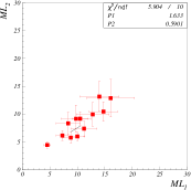
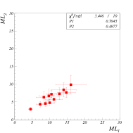
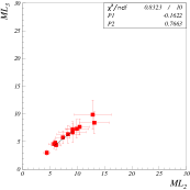
The too low , especially for the vs plot reveal that the three methods are not independent.
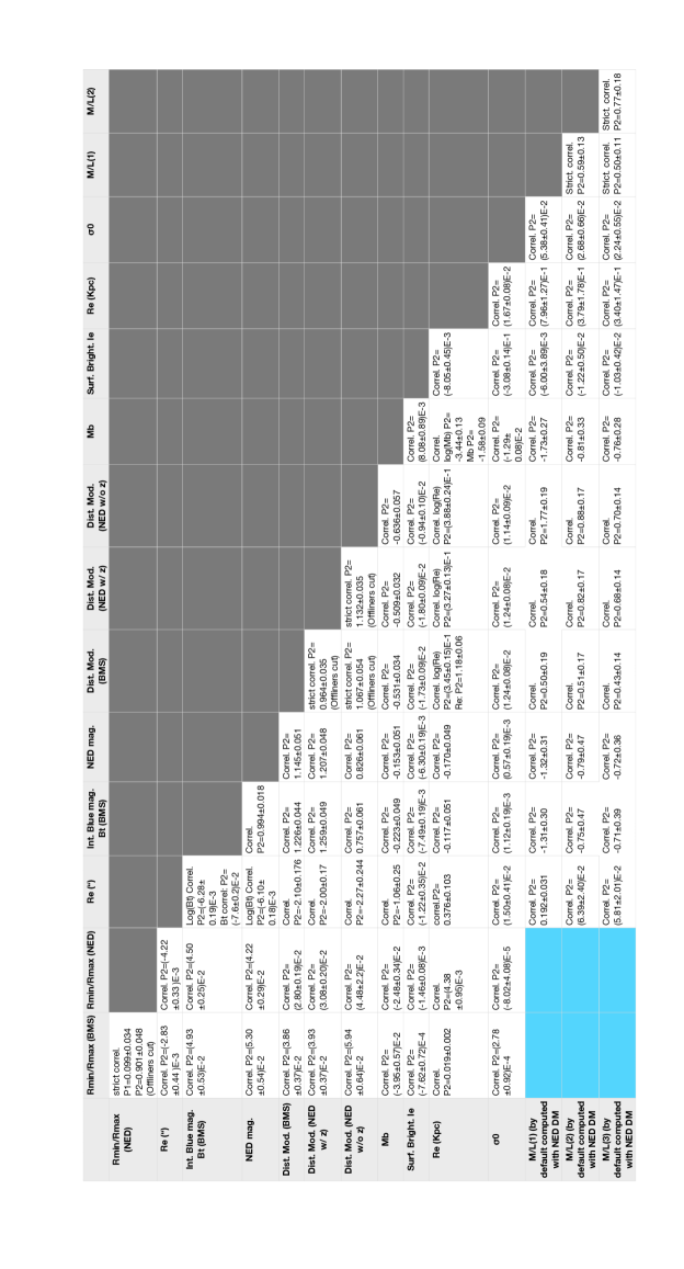
L.3.3 Discussion
A correlation summary is given in the table on page 88. The observed clear correlations are shown in Fig. 89. Possible weak correlations are shown in Fig. 90.
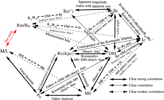

In most cases the are larger than 1. This is mostly because a linear fit is ill-suited to fit the data, and because two correlated variables can depend= on other variables, which adds an additional non-gaussian dispersion. For example we already mentioned that the vs correlation has an additional variable, the (unknown) projection angle of the ellipsoid to the observed ellipse, which creates an additional dispersion.
All in all, the clear correlations seen in this section can all be classified as:
-
•
Physical correlations;
-
•
Observational biases;
-
•
Unexplained but known correlations related to galaxy structure (e.g. Kormendy, Faber-Jackson relations…).
This is satisfactory since this clarifies how to account, if necessary, for the important correlations.
L.4 Corrections
L.4.1 Corrections for measurement biases
We will ignore the weak uncertain correlations shown in Fig. 90. Measurement biases seem to be directly at the origin of the and correlations. Measurement biases seem to be indirectly at the origin of the , and correlations. Finally, measurement biases seem to be indirectly contributing partly to the , , , , and correlations. Unsurprisingly, is involved in all the measurement biases.
In order to study the effect of on the dependence with , we bin and plot in function of for each of the bins. The results for the linear fits made for each bin are shown in Fig. 91. We choose bins of size 1, or smaller if the statistics is large. We use and values from [3]. The values of and in function of the bins can be seen on the left panel of Fig. 92. Within the approximation of a linear dependence of in function of , then . Thus, is our quantity of interest. Except for one outlying point, there is no strong dependence of and with : we find for a reduced . This would suggest that the correction for the bias would increase the significance of our quantity of interest . Figs. 91 and 92 also suggest that there is something wrong with bin (possibly because of the lowest point (galaxy NGC 4510) that has very small error171717This small error is partly an artifact: Ref. [3] gives relative errors, hence small values have small absolute errors, which might not reflect fully the uncertainty. Apart from re-performing a full error analysis, there is no easy way to correct this effect. We also refrain from removing this particular galaxy (NGC 4510) after close-up study: most of galaxies would have a particularity after close examination that one could use to justify excluding it from our sample. It would be thus possible to bias the result of our study in any arbitrary way. Obeying our general criteria and basic statistics rules protects us from such bias. ). The right panel of Fig. 92 shows the fit result with bin excluded. We find similar fit values: for a reduced . The value of the reduced , closer to the expected 1, supports excluding bin .
The correction for the bias would increase by a factor (here, -13.00 is the value of at =32.5). However, this assumes the reliability of a linear extrapolation over 31 units of , based on a fit performed over a range of 4.5 units. Such a procedure would yield average values of ( coefficient of the top plots of Fig. 92), a value 6 times larger than the average 13.3 for our data sample. Assuming similar effect, the bias correction would be reduced to . This is still a large correction and given the uncertainties attached to it and the fact that ignoring it would reduce the signature of the correlation we are investigating, we choose to not apply the correction. However, we do retain the fact that bin should be excluded from our analysis. The resulting linear fit of vs is (Fig. 93), to be compared to the result shown in Fig. 67 (). The Pearson coefficient calculated when keeping data with uncertainties is -0.44 (the linear fit becomes ). When keeping data with the Pearson coefficient becomes -0.64 (the linear fit becomes ). Those indicate a large correlation.
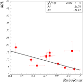
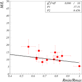
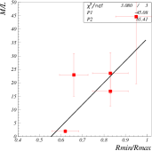
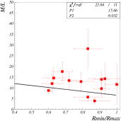
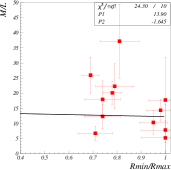
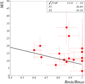
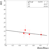
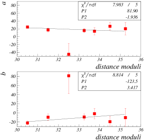
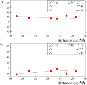
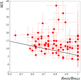
L.4.2 Surface brightness vs absolute blue magnitude
We exclude from the sample the two galaxies that are close to the dwarf elliptical locus, see Section L.3.2 (we apply a selection at ). This has no significant consequence on the vs relation: compare Fig. 94 to Fig. 93. The linear fit result is . Because this correction has little effect, we do not apply it in the rest of the analysis.
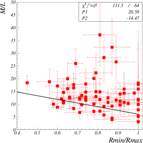
L.4.3 Hubble parameter correction
We must scale the slope of our assumed relation between and to account for the fact that [3] uses a large value of the Hubble parameter . This should be corrected for since redshift distances scale inversely to and scales inversely with distances. Using =70 km s-1 Mpc-1 instead of the 95 km s-1 Mpc-1 used in [3] yields a correction of . The linear fit becomes .
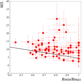
L.4.4 Projection correction
L.5 Final result
The final result including the projection correction, the Hubble parameter correction and the exclusion of bin but without applying the distance modulus bias correction (that would enhance further the dependence with ) is shown in Fig. 96. Also excluded are the possible corrections discussed in Figs. 65, 66 and 73 (this is a conservative choice since this would enhance further the dependence with ). Fig. 96 can be compared to Figs. 67, 93 and 95 that show the different stages of the analysis. The best linear fit yields , with a . This is a strong positive signature with a 13 signal. The Pearson correlation coefficient is 0.87, or 0.91 after removing the galaxies with (uncorrected) uncertainty above or respectively, see Fig. 97. In all cases, it indicates a strong correlation. Again, it is interesting to notice that if we select the highest precision data, then the vs correlation is enhanced, both for the determination using of the Pearson criterion and for the determination from the linear fit parameter .
