Batch-sequential design and heteroskedastic surrogate modeling for delta smelt conservation

Abstract

Delta smelt is an endangered fish species in the San Francisco estuary that have shown an overall population decline over the past 30 years. Researchers have developed a stochastic, agent-based simulator to virtualize the system, with the goal of understanding the relative contribution of natural and anthropogenic factors that might play a role in their decline. However, the input configuration space is high-dimensional, running the simulator is time-consuming, and its noisy outputs change nonlinearly in both mean and variance. Getting enough runs to effectively learn input–output dynamics requires both a nimble modeling strategy and parallel evaluation. Recent advances in heteroskedastic Gaussian process (HetGP) surrogate modeling helps, but little is known about how to appropriately plan experiments for highly distributed simulation. We propose a batch sequential design scheme, generalizing one-at-a-time variance-based active learning for HetGP, as a means of keeping multi-core cluster nodes fully engaged with runs. Our acquisition strategy is carefully engineered to favor selection of replicates which boost statistical and computational efficiency when training surrogates to isolate signal from noise. Design and modeling are illustrated on a range of toy examples before embarking on a large-scale smelt simulation campaign and downstream high-fidelity input sensitivity analysis.

Keywords: Gaussian process surrogate modeling, agent-based model, active learning, input-dependent noise, replication, sensitivity analysis

1 Introduction

Delta smelt is a short-lived fish species that spends its entire life within the San Francisco Estuary (SFE) that connects the Sacramento and San Joaquin Rivers through the Bay into the Pacific Ocean. The SFE has undergone many changes over the past 150 years due to human development. It is now a network of channels and sloughs surrounding islands protected by a man-made levee system (Lund et al.,, 2010). Since 1960, environmental and ecological conditions (including delta smelt populations) have been extensively monitored. Derived population indices for delta smelt have shown a general decline since about 1980. In 1993 they were listed as threatened under the US Endangered Species Act. The population exhibited a large drop in 2000 and has remained at low abundance (Stompe et al.,, 2020). Factors that may contribute to the decline of delta smelt include entrainment by water diversion facilities, changes in food base and predation pressure, pollution, and changes in habitat related to salinity and turbidity (Baxter et al.,, 2015; Moyle et al.,, 2016).

Identifying the relative importance of factors that impact the delta smelt population is important for designing effective management actions to balance human water use and maintenance/recovery of the species. Diverse statistical/observational analyses have been entertained (Thomson et al.,, 2010; MacNally et al.,, 2010; Miller et al.,, 2012; Maunder and Deriso,, 2011; Hamilton and Murphy,, 2018). Rose et al., (2013a, b) developed a spatially-explicit, agent-based model (ABM) of delta smelt to examine such factors. The model simulates daily growth, mortality, reproduction, and movement of hundreds of thousands of agents (smelt) from their birth to death. By explicitly representing food (zooplankton), temperature, salinity, and water velocities experienced by agents based on their location within a hydrodynamics grid, the ABM attempts to scale local environmental effects up to population-level responses. Simulations under myriad environmental and system variables enabled the authors to identify conditions both detrimental and conducive to smelt growth and survival, and to compare how changes in food and in entrainment from water diversion facilities affect population growth rates (Kimmerer and Rose,, 2018). Ultimately, the goal of such simulation is to augment and complement statistical models, and to assist in determining which environmental factors could affect the population of delta smelt.

Rose et al., (2013a, b)’s ABM is coded in Fortran and the version we use takes about six hours to run. Even after pre-selecting a subset of key model parameters, the input configuration space is large (upwards of 13-dimensions), and the outcome of the simulator varies across random seeds. Response surface learning with this stochastic computer model – separating signal from noise in a high dimensional space – requires a large, and costly, distributed HPC simulation campaign and pairing with a flexible meta model. In our initial study, described in Section 2.3, we observe that the response surface is nonlinear and heteroskedastic, i.e., sensitivity to stochastic simulation dynamics is not uniform in the input space. These features challenge effective meta-modeling, which are essential for downstream tasks like input sensitivity analysis, mirroring ones which are increasingly common the analysis of stochastic simulation experiments (Baker et al.,, 2020).

In similar but simpler situations (e.g., Johnson,, 2008; Bisset et al.,, 2009; Farah et al.,, 2014; Fadikar et al.,, 2018; Rutter et al.,, 2019) – being not as extreme as the delta smelt ABM in terms of simulator cost, input dimension, and changing variance – researchers have been getting mileage out of methods for surrogate modeling and the design and analysis of computer experiments (Sacks et al.,, 1989; Santner et al.,, 2018; Gramacy,, 2020). Default, model-free design strategies, such as space-filling Latin hypercube samples (LHS; Mckay et al.,, 1979), are a good starting point but are not reactive/easily refined to target parts of the input space which require heavier sampling. Model-based designs based on Gaussian process (GP) surrogates fare better, in part because they can be developed sequentially along with learning (e.g., Jones et al.,, 1998; Seo et al.,, 2000; Gramacy and Polson,, 2011).

Until recently, surrogate modeling and computer experiment design methodology has emphasized deterministic computer evaluations, for example those arising in finite element analysis or solving systems of differential equations. Sequential design with heteroskedastic GP (HetGP) surrogates (Binois et al.,, 2018a) for stochastic simulations has recently been proposed as a means of dynamically allocating more runs in higher uncertainty regions of the input space (Binois et al.,, 2019). Such schemes are typically applied as one-at-a-time affairs – fit model, optimize acquisition criteria, run simulation, augment data, repeat – which would take too long for the delta smelt model. We anticipate needing thousands of runs, with several hours per run. That process cannot be fully serial.

Batch-sequential design procedures have been applied with GP surrogates (e.g. Loeppky et al.,, 2010; Ginsbourger et al.,, 2010; Chevalier,, 2013; Duan et al.,, 2017; Erickson et al.,, 2018). These attempt to calculate a group of runs to go at once, say on a multi-core supercomputing node, towards various design goals. Quasi-batch schemes, which asynchronously re-order points for an unknown number of future simulations have also thrived in HPC environments (Gramacy and Lee,, 2009; Taddy et al.,, 2009). However, none of these schemes explicitly address input-dependent noise like we observe in the delta smelt ABM simulations. Here we propose extending the one-at-a-time method of Binois et al., (2019) to a batch-sequential setting. Our goal is to design for batches of size 24 to match the number of cores available on nodes of a supercomputing cluster at Virginia Tech. Following Binois et al.,’s lead, we develop a novel scheme for encouraging replicates in the batches. Replication is a tried and true technique for separating signal from noise, reducing sufficient statistics for modeling and thus enhancing computational and learning efficiency.

Our flow is as follows. Section 2 reviews simulation, surrogate modeling and design elements for delta smelt simulations. We also describe a pilot study on a reduced input space identifying challenges/appropriate modeling elements and motivating a HetGP framework. Section 3 explains our innovative batch-sequential acquisition strategy through an integrated mean-squared prediction error (IMSPE) criteria and closed-form derivatives for optimization, extending the one-at-a-time process from Binois et al., (2019). Section 4 provides a novel and thrifty post-processing scheme to identify replicates in the new batch. Illustrative examples are provided throughout, and Section 5 details a benchmarking exercise against the infeasible one-at-a-time gold standard. Finally, in Section 6 we apply the design method to smelt simulations (in a larger space), collecting thousands of runs utilizing tens of thousands of core hours across a several weeks-long simulation campaign. Those runs are used to conduct a sensitivity analysis to exemplify potential downstream tasks. We conclude with other suggestions and methodological ideas in Section 7.

2 Problem description and solution elements

Here we describe the smelt simulator and HPC implementation, review surrogate modeling elements and report on a pilot study, motivating our methodological developments.

2.1 Agent-based model

The delta smelt population model of Rose et al., (2013a) is a stochastic, spatially-explicit, agent-based model (ABM). It tracks reproduction, growth, mortality, and movement of individual fish through life stages. Agents move around within a 1d network of channels and nodes formed by rivers and leveed islands. Daily values of environmental variables of water temperature, salinity, and the densities of six zooplankton prey types drive the model. These vary daily and spatially among channels over a grid. In our simulations, these drivers are based on observed environmental variables from 1995 to 2005 to allow exploration of potential factors influencing a population decline starting around 2000.

The model assumes that factors impact the agents in specific ways. Temperature and zooplankton affect daily growth, whereas hydrodynamic transport and salinity affect movement. Daily mortality is comprised of stage-specific rates (mostly predation), starvation, and entrainment of individuals by water diversion facilities. Daily egg production is used to start agents as yolk-sac larvae. Upon progressing through multiple life stages and reaching maturity, individuals spawn a year later, and the cycle repeats year-after-year. Stochastic calculations within a run include: realization of zooplankton concentrations in channels each day from regional means, assignment of temperature of spawning to adults, aspects of hourly water transport of larvae and the twice-per-day movement of juveniles and adults, timing of upstream and downstream spawning migration, and selection of channels when individuals are moved out of nodes (reservoirs).

symbol	parameter	description	range	default	pilot study
$m_{y}$	zmorty	yolk-sac larva MR	[0.01,0.50]	0.035	0.035
$m_{l}$	zmortl	larval MR	[0.01, 0.08]	0.050	0.050
$m_{p}$	zmortp	post-larval MR	[0.005, 0.05]	0.030	0.030
$m_{j}$	zmortj	juvenile MR	[0.001, 0.025]	0.015	[0.005,0.030]
$m_{a}$	zmorta	adult MR	[0.001, 0.01]	0.006	0.006
$m_{r}$	middlemort	river entrain MR	[0.005, 0.05]	0.020	[0, 0.05]
$P_{l,2}$	preyk(3,2)	larvae EPT 2	[0.10, 20.0]	0.200	0.200
$P_{p,2}$	preyk(4,2)	postlarvae EPT 2	[0.10, 20.0]	0.800	[0.10, 1.84]
$P_{p,6}$	preyk(4,6)	postlarvae EPT 6	[0.10, 20.0]	1.500	$P_{p,2}$
$P_{j,3}$	preyk(5,3)	juveniles EPT 3	[0.10, 20.0]	0.600	[0.1, 1.5]
$P_{j,6}$	preyk(5,6)	juveniles EPT 6	[0.10, 20.0]	0.600	$P_{j,3}$
$P_{a,3}$	preyk(6,3)	adults EPT 3	[0.01, 20.0]	0.070	0.070
$P_{a,4}$	preyk(6,4)	adults EPT 4	[0.01, 5.0]	0.070	0.070

Table 1: Smelt simulator inputs considered in this analysis. The pilot study column indicates settings for Section 2.3. MR is mortality rate; EPT means eating prey type.

The Rose et al. ABM has more than fifty model parameters. We selected 13 of these to focus on in this analysis because they are known to be important to model dynamics and have direct relevance to the ecology and management of delta smelt. They are listed in Table 1 with their symbols and input parameter name, descriptions, range extremes, default/calibrated values, and spans considered in our pilot study (Section 2.3).

The first set of parameters in Table 1 involve natural mortality rates assigned to each life stage. While there is uncertainty in these values, feasible ranges can be deduced from prior analysis and review of values reported in the literature. The second group is a single parameter ($m_{r}$) that modifies the mortality rate of juvenile and adults based on whether river flows in the Delta subregion are transporting individual fish toward or away from water diversion facilities. Flows towards facilities result in the addition of $m_{r}$ due to entrainment.

The third group of parameters are feeding-related and are specific to prey group and life stage; for example, $P_{j,6}$ is juveniles feeding on prey type 6 (Pseudodiaptomus forbesi). The parameters are half-saturation coefficients in a functional response feeding relationship and so larger values reduce feeding rates. Prey types are selected for each life stage that were dominant in simulated diets for the time period analyzed here (Rose et al.,, 2013a). Dependencies are created among feeding parameters to mimic the effects of more or less food available to life stages that consume multiple prey types. For example, when $P_{p,2}$ is varied its value is pegged to $P_{p,6}$, i.e., more or less food for post-larval stage. These dependencies are noted in Table 1 for the pilot study and Table 2 for the full analysis.

A distinct feature of the Rose et al., (2013a) ABM is how model behavior is summarized. Output is extensive because the model generates size (length and weight), location, growth rate, mortality from different sources, diet, and other individual-level attributes every day for approximately 450,000 model individuals for the ten-year simulations analyzed here. Rose et al., (2013a) summarize these dynamics using the information on individuals to estimate a matrix projection model for each year, ultimately generating a population growth rate ($\lambda_{i}$) each year. Here, we use the geometric mean of growth rates from 1995 to 2004 as a convenient scalar output summarizing results of the 10-year simulation: $\lambda=(\prod_{i=1995}^{2004}\lambda_{i})^{1/10}\!$. The value of $\lambda$ is an indicator of the health of the population of delta smelt over the time period of the simulation and is directly interpretable. Values greater than one indicate population growth over the 10 years; values less than one indicate decline.

Previous simulation campaigns did not systematically vary all the parameters simultaneously. For example, the importance of single factors were estimated by evaluating population changes after structurally eliminating that factor in the simulation(s) (Kimmerer and Rose,, 2018). This is very different from a Saltelli-style/functional analysis of variance (e.g., Saltelli et al.,, 2000; Oakley and O’Hagan,, 2004; Marrel et al.,, 2009; Gramacy,, 2020, Chapter 8.2) favored by the computer surrogate modeling literature. That and other downstream applications require a meta-modeling design strategy in the face of extreme computational demands and stochasticity over random seeds.

2.2 Surrogate modeling

We regard the delta smelt simulator as an unknown function $f:\mathbb{R}^{d}\rightarrow\mathbb{R}$. A meta-model $\hat{f}$ fit to evaluations $(\mathbf{x}_{i},y_{i}\sim f(\mathbf{x}_{i}))$, for $i=1,\dots,N$ is known as a surrogate model or emulator (Gramacy,, 2020). The idea is that fast $\hat{f}(\mathbf{x})$ could be used in lieu of slow/expensive $f(\mathbf{x})$ for downstream applications like input sensitivity analysis. Although there are many sensible choices, the canonical surrogate is based on Gaussian processes (GPs). If $f$ is deterministic ($y_{i}=f(\mathbf{x}_{i})$), this amounts to specifying a multivariate normal (MVN) for $\mathbf{Y}_{N}=(y_{1},\dots,y_{N})^{\top}$: $\mathbf{Y}_{N}\sim\mathcal{N}_{N}(\mathbf{0},{\color[rgb]{0,0,0}\tau^{2}}\mathbf{C}_{N})$. Defining $\mathbf{C}_{N}$ based on distance,

$$\mathbf{C}_{N}^{ij}=c_{\boldsymbol{\theta}}(\mathbf{x}_{i},\mathbf{x}_{j})=\exp\left\{-\sum_{k=1}^{d}\frac{(\mathbf{x}_{ik}-\mathbf{x}_{jk})^{2}}{\theta_{k}}\right\},$$

provides smooth decay in function space when moving apart in $\mathbf{x}$-space and yields a predictive surface interpolates the data. Fixing $\boldsymbol{\theta}$ and $\tau^{2}$, dropping $\boldsymbol{\theta}$ in $c_{\boldsymbol{\theta}}(\cdot,\cdot)$, extending the MVN to the cover $(N+N^{\prime})$-sized $(\mathbf{Y}_{N},\mathcal{Y}(\mathcal{X}))$ at training inputs $\mathbf{X}_{N}$ and $N^{\prime}$ testing sites $\mathcal{X}$, and MVN conditioning leads to a Gaussian predictive distribution $\mathcal{Y}(\mathcal{X})\mid\mathbf{Y}_{N}$ with

mean $$\mu(\mathcal{X}\mid\mathbf{Y}_{N}) =c(\mathcal{X},\mathbf{X}_{N})\mathbf{C}_{N}^{-1}\mathbf{Y}_{N},$$ (1)

and variance $$\Sigma(\mathcal{X}\mid\mathbf{Y}_{N}) =\tau^{2}[c(\mathcal{X},\mathcal{X})-c(\mathcal{X},\mathbf{X}_{N})\mathbf{C}_{N}^{-1}c(\mathcal{X},\mathbf{X}_{N})^{\top}].$$

Observe that uncertainty $\Sigma(\mathcal{X}\mid\mathbf{Y}_{N})$ is a quadratic function of distance between testing data $\mathcal{X}$ and training data $\mathbf{X}_{N}$ locations. For this reason, space-filling designs such as maximin design (Johnson et al.,, 1990), LHS and hybrids thereof like maximin–LHS (Morris and Mitchell,, 1995) are common in order to sufficiently cover the input space.

For stochastic $f$ with constant noise we can add a nugget term $g$ to the diagonal $\mathbf{K}_{N}=\mathbf{C}_{N}+\boldsymbol{\Lambda}_{N}$ for $\boldsymbol{\Lambda}_{N}=g\mathbb{I}_{N}$ and take $\mathbf{Y}_{N}\sim\mathcal{N}_{N}(0,\tau^{2}\mathbf{K}_{N})$. To model a response surface with non-constant noise, Binois et al., (2018a) proposed freeing the diagonal elements of $\boldsymbol{\Lambda}_{N}$ under a smoothness penalty. They call this a heteroskedastic GP (HetGP). Specifically, let $\delta_{1},\delta_{2},\dots,\delta_{n}$ denote latent nuggets, corresponding to $n\ll N$ unique design locations. Replication in a design, here with degree $N-n$, is essential for separating signal from noise and also leads to computational efficiencies, working with cubic in $n$ rather than $N$ flops through a Woodbury trick not reviewed here. Place $\delta_{1},\delta_{2},\dots,\delta_{n}$ diagonally in $\mathbf{\Delta}_{n}$ and assign to these a structure similar to $\mathbf{Y}$ but now encoding a prior on variances: $\boldsymbol{\Delta}_{n}\sim\mathcal{N}_{n}(\mathbf{0},\tau^{2}_{(\boldsymbol{\delta})}(\mathbf{C_{(\boldsymbol{\delta})}}+g_{(\boldsymbol{\delta})}\mathbf{A}_{n}^{-1}))$. $\mathbf{C_{(\boldsymbol{\delta})}}$ is the covariance matrix of $n$ unique design locations defined under similar kernel/inverse distance structure; $\mathbf{A}_{n}$ is a diagonal matrix, $\mathbf{A}_{ii}=a_{i}$, which denotes the number of replicates at unique location $\bar{\mathbf{x}}_{i}$ so that $\sum_{i=1}^{n}a_{i}=N$; $g_{(\boldsymbol{\delta})}$ is a “nugget of nuggets” controlling the smoothness of $\lambda_{i}$’s relative to $\delta_{i}$’s. Smoothed $\lambda_{i}$-values can be calculated by plugging $\boldsymbol{\Delta}_{n}$ into GP mean predictive equations (1):

$$\boldsymbol{\Lambda}_{n}=\mathbf{C_{(\boldsymbol{\delta})}}\mathbf{K}_{(\boldsymbol{\delta})}^{-1}\boldsymbol{\Delta}_{n},\quad\mbox{ where }\quad\mathbf{K}_{(\boldsymbol{\delta})}=\mathbf{C_{(\boldsymbol{\delta})}}+g_{(\boldsymbol{\delta})}\mathbf{A}_{n}^{-1}.$$ (2)

Parameters including $\boldsymbol{\theta},\tau^{2}$ for both GPs, i.e., for mean and variance, and latent nuggets $\boldsymbol{\Delta}_{n}$ may be estimated by maximizing the joint log likelihood with derivatives in time cubic in $n$. Software is available for R as hetGP on CRAN (Binois et al.,, 2018a).

2.3 Pilot study

To assist with R-based surrogate modeling we built a custom R interface to the underlying Fortran program automating the passing of input configuration files/parsing of outputs through ordinary function I/O. The Rmpi package (Yu,, 2002) facilitates cluster-level parallel evaluation for distributed simulation through a message passing interface (MPI) on our Advanced Research Computing (ARC) HPC facility at Virginia Tech.

To test that interface and explore modeling and design options we ran a limited delta smelt simulation campaign over six parameters (inputs) under a maximin–LHS of size $n=96$ (via lhs; Carnell,, 2020) with five replicates for each combination. Juvenile and river entrainment mortalities $m_{j}$ and $m_{r}$ were varied over their ranges with the rest of the mortality rate parameters were fixed at their default values from Table 1. Post-larvae $(P_{p,2})$ and juvenile $(P_{j,3})$ prey parameters for zooplankton type 2 are allowed to vary over their ranges with value of $P_{p,2}$ also being assigned to $P_{p,6}$ and value of $P_{j,3}$ also being assigned to $P_{j,6}$ ($P_{p,2}=P_{p,6}$ and $P_{j,3}=P_{j,6}$). Other prey types were fixed to their default settings making the effective input dimension four. Twenty 24-core VT/ARC cluster nodes were fully occupied in parallel in order to get all $N=480$ runs in about six hours.

mean surface	variance surface	1d predictive bands

Figure 1: 2d heatmap and 1d lineplot slices of predictive mean and variance for selected inputs. The numbers overlaid indicate design locations and numbers of replicates.

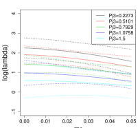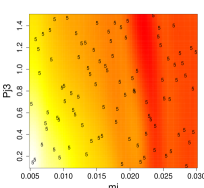
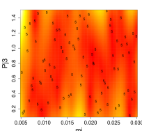
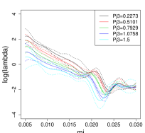
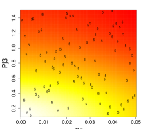
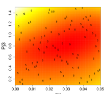
We fit the simulation data using hetGP with inputs $\mathbf{X}_{N}$ coded to the unit cube $[0,1]^{4}$ and with $\mathbf{Y}_{N}$ derived from $\log\lambda_{i}$, the (log) 10-year geometric average of the population growth rate, for $i=1,\dots,480$ using $y_{i}\equiv-6\log 10$ in the few cases where $\lambda_{i}=0$ was returned. As a window into visualizing the fitted response surface we plotted a selection of 1d and 2d predictive mean error/variance slices in Figure 1, using defaults from Table 1 for the fixed variables. The first and second row correspond to subspaces $(P_{j,3}\times m_{j})$ and $(P_{j,3}\times m_{r})$, respectively. Observe in the middle column how noise intensity changes over the 2d input subspace, indicating heteroskedasticity. Both mean and variance surfaces are nonlinear. A similar, higher resolution view is offered by the 1d slices in the final column. The solid curves in the top-right panel are horizontal slices of the top left panel with $P_{j,3}$ fixed at five different values, and analogously on the bottom-right. Predictive intervals, with 95% nominal coverage, are shown as dashed lines. In both views, the width of dashed predictive band changes, sometimes drastically, as $m_{j}$ and $m_{r}$ are increased. Clearly $m_{j}$ in the top-right panel shows more dramatic and nonlinear mean and variance effects.

3 Batch sequential design

The plan is to scale-up the pilot study of Section 2.3 and vary more quantities in the 13d input space. Ideally, sampling effort would concentrate on parts of the input space that are harder to model, or where more value can be extracted from noisy simulations. Binois et al., (2019) proposed IMSPE-based one-at-a-time sequential design with that goal in mind. Here we extend that to batches that can fill entire compute nodes at once.

3.1 A criterion for minimizing variance

Integrated mean-squared prediction error (IMSPE) measures how well a surrogate model captures input–output relationships. It is widely used as data acquisition criterion; see, e.g., Gramacy, (2020, Chapters 6 and 10). Let $\check{\sigma}^{2}_{N}(\mathbf{x})$ denote the nugget free predictive variance for any single $\mathbf{x}\in D$. IMSPE for a design $\mathbf{X}_{N}$ may be defined as:

$$I_{N}\equiv\text{IMSPE}(\mathbf{X}_{N})=\int\limits_{\mathbf{x}\in D}\check{\sigma}^{2}_{N}(\mathbf{x})\,d\mathbf{x}=\int\limits_{\mathbf{x}\in D}\hat{\tau}^{2}[c(\mathbf{x},\mathbf{x})-c(\mathbf{x},\mathbf{X}_{N})\mathbf{K}_{N}^{-1}c(\mathbf{x},\mathbf{X}_{N})^{\top}]\,d\mathbf{x}.$$

The integral above has an analytic expression for GP surrogates, in part because of the closed form for $\check{\sigma}^{2}_{N}(\mathbf{x})$. Examples involving specialized GP setups in recent literature include Ankenman et al., (2010); Leatherman et al., (2017); Chen et al., (2019). Similar expressions do not, to our knowledge, exist for other popular surrogates like deep neural networks, say.

Binois et al., (2019) gives perhaps the most generic and prescriptive expression for GPs, emphasizing replicates at $n\ll N$ unique inputs $\bar{\mathbf{x}}_{i}$ for computational efficiency. Let $\mathbf{K}_{n}$ denote the unique $n\times n$ covariance structure comprised of $\mathbf{K}_{n}^{ij}=c(\bar{\mathbf{x}}_{i},\bar{\mathbf{x}}_{j})+\delta_{ij}\frac{r(\bar{\mathbf{x}}_{i})}{a_{i}}$. Let $\mathbf{W}_{n}$ be an $n\times n$ matrix with entries comprising integrals of kernel products $w(\bar{\mathbf{x}}_{i},\bar{\mathbf{x}}_{j})=\int_{\mathbf{x}\in D}c(\bar{\mathbf{x}}_{i},\mathbf{x})c(\bar{\mathbf{x}}_{j},\mathbf{x})\;d\mathbf{x}$ for $1\leq i,j\leq n$, and let $E=\int_{\mathbf{x}\in D}{\color[rgb]{0,0,0}\hat{\tau}^{2}}c(\mathbf{x},\mathbf{x})\;d\mathbf{x}$, which is constant with respect to the design $\mathbf{X}_{n}$. Closed forms are provided in Appendix B of Binois et al., for common kernels. Then $\mathcal{O}(n^{3})$ calculations yield

$$I_{N}=\mathbb{E}[{\color[rgb]{0,0,0}\hat{\tau}^{2}}c(X,X)]-\mathbb{E}[{\color[rgb]{0,0,0}\hat{\tau}^{2}}c(X,\mathbf{X}_{N})\mathbf{K}_{N}^{-1}c(X,\mathbf{X}_{N})^{\top}]=E-{\color[rgb]{0,0,0}\hat{\tau}^{2}}\operatorname{tr}(\mathbf{K}_{n}^{-1}\mathbf{W}_{n}).$$ (3)

Although expressed for an entire design $\mathbf{X}_{n}$, in practice IMSPE is most useful in sequential application where the goal is to choose new runs. Binois et al., provided a tidy expression for solving for $\mathbf{x}_{n+1}$ by optimizing $I_{n+1}(\tilde{\mathbf{x}})$ over $n+1^{\mathrm{st}}$ candidates $\tilde{\mathbf{x}}$. We extend this to an entire batch of size $M\geq 1$, augmenting $\mathbf{X}_{N}$ or (more compactly) the unique elements $\bar{\mathbf{X}}_{n}$. Let $\widetilde{\mathbf{X}}=\{\tilde{\mathbf{x}}_{1},\tilde{\mathbf{x}}_{2},\dots,\tilde{\mathbf{x}}_{M}\}^{\top}$ denote the coordinates of a new batch. Let $I_{N+M}(\widetilde{\mathbf{X}})$ denote the new IMSPE, which is realized most directly by shoving a row-combined $[\mathbf{X}_{N};\widetilde{\mathbf{X}}]$ into Eq. (3). That over-simplifies, and flops in $\mathcal{O}((N+M)^{3})$ could be prohibitive.

Partition inverse equations (Barnett,, 1979) can be leveraged for even thriftier evaluation. Extend the kernel $\mathbf{K}$ and its integral $\mathbf{W}$ to define new $(n+M)\times(n+M)$ matrices

$$\mathbf{K}_{n+M}=\begin{bmatrix}\mathbf{K}_{n}&c({\bar{\mathbf{X}}_{n}},\widetilde{\mathbf{X}})\\ c({\bar{\mathbf{X}}_{n}},\widetilde{\mathbf{X}})^{\top}&c(\widetilde{\mathbf{X}},\widetilde{\mathbf{X}})+r(\widetilde{\mathbf{X}})\end{bmatrix},\quad\mathbf{W}_{n+M}=\begin{bmatrix}\mathbf{W}_{n}&w({\bar{\mathbf{X}}_{n}},\widetilde{\mathbf{X}})\\ w({\bar{\mathbf{X}}_{n}},\widetilde{\mathbf{X}})^{\top}&w(\widetilde{\mathbf{X}},\widetilde{\mathbf{X}})\end{bmatrix},$$

where $\mathbf{W}_{n}=w({\bar{\mathbf{X}}_{n}},{\bar{\mathbf{X}}_{n}})$ and $r(\widetilde{\mathbf{X}})=\mathrm{Diag}(r(\tilde{\mathbf{x}}_{1}),\dots,r(\tilde{\mathbf{x}}_{M}))$ comes from smoothed latent variances following Eq. (2) via $c_{(\boldsymbol{\delta})}(\widetilde{\mathbf{X}},{\bar{\mathbf{X}}_{n}})$ so that

$${\color[rgb]{0,0,0}r}(\widetilde{\mathbf{X}})={\color[rgb]{0,0,0}c}_{(\boldsymbol{\delta})}(\widetilde{\mathbf{X}},{\bar{\mathbf{X}}_{n}})(\mathbf{C_{(\boldsymbol{\delta})}}+g_{(\delta)}\mathbf{A}_{n}^{-1})^{-1}\boldsymbol{\Delta}_{n}.$$ (4)

Given $\mathbf{K}_{n}^{-1}$, we may fill the inverse $\mathbf{K}_{n+M}^{-1}$ in flops in $\mathcal{O}(M^{3}+nM^{2}+n^{2}M)$ as

$$\mathbf{K}_{n+M}^{-1}=\begin{bmatrix}\mathbf{K}_{n}^{-1}+g(\widetilde{\mathbf{X}})\Sigma(\widetilde{\mathbf{X}})g(\widetilde{\mathbf{X}})^{\top}&g(\widetilde{\mathbf{X}})\\ g(\widetilde{\mathbf{X}})^{\top}&\Sigma(\widetilde{\mathbf{X}})^{-1}\end{bmatrix},$$ (5)

where $g(\widetilde{\mathbf{X}})=-\mathbf{K}_{n}^{-1}c(\mathbf{X}_{n},\widetilde{\mathbf{X}})\Sigma(\widetilde{\mathbf{X}})^{-1}$, $\Sigma(\widetilde{\mathbf{X}})=r(\widetilde{\mathbf{X}})+c(\widetilde{\mathbf{X}},\widetilde{\mathbf{X}})-c({\bar{\mathbf{X}}_{n}},\widetilde{\mathbf{X}})^{\top}\mathbf{K}_{n}^{-1}c({\bar{\mathbf{X}}_{n}},\widetilde{\mathbf{X}})$. Multiplying through components of Eq. (5) and properties of traces in Eq. (3) leads to

$$I_{N+M} =E-{\color[rgb]{0,0,0}\hat{\tau}^{2}}\operatorname{tr}(\mathbf{K}_{n}^{-1}\mathbf{W}_{n}+g(\widetilde{\mathbf{X}})\Sigma(\widetilde{\mathbf{X}})g(\widetilde{\mathbf{X}})^{\top}+g(\widetilde{\mathbf{X}})w(\mathbf{X}_{n},\widetilde{\mathbf{X}})^{\top})$$

$$\quad-{\color[rgb]{0,0,0}\hat{\tau}^{2}}\operatorname{tr}(g(\widetilde{\mathbf{X}})^{\top}w(\mathbf{X}_{n},\widetilde{\mathbf{X}})+\Sigma(\widetilde{\mathbf{X}})^{-1}w(\widetilde{\mathbf{X}},\widetilde{\mathbf{X}}))$$ (6)

$$=I_{N}-{\color[rgb]{0,0,0}\hat{\tau}^{2}}\left[\operatorname{tr}(g(\widetilde{\mathbf{X}})\Sigma(\widetilde{\mathbf{X}})g(\widetilde{\mathbf{X}})^{\top})+2\operatorname{tr}(g(\widetilde{\mathbf{X}})w(\mathbf{X}_{n},\widetilde{\mathbf{X}})^{\top})+\operatorname{tr}(\Sigma(\widetilde{\mathbf{X}})^{-1}w(\widetilde{\mathbf{X}},\widetilde{\mathbf{X}}))\right].$$

Finding the best $\widetilde{\mathbf{X}}$ requires only the latter term above. That is, we seek

$$\widetilde{\mathbf{X}}^{*} =\mathrm{argmax}_{\widetilde{\mathbf{X}}\in D}\operatorname{tr}(g(\widetilde{\mathbf{X}})\Sigma(\widetilde{\mathbf{X}})g(\widetilde{\mathbf{X}})^{\top})+2\operatorname{tr}(g(\widetilde{\mathbf{X}})w(\mathbf{X}_{n},\widetilde{\mathbf{X}})^{\top})+\operatorname{tr}(\Sigma(\widetilde{\mathbf{X}})^{-1}w(\widetilde{\mathbf{X}},\widetilde{\mathbf{X}})).$$

In other words, we seek $\widetilde{\mathbf{X}}^{*}$ giving the largest reduction in IMSPE. Evaluation involves flops in the orders quoted above, however in repeated calls for numerical optimization many of the $\mathcal{O}(n)$ quantities can be pre-evaluated leaving $\mathcal{O}(M^{3}+nM^{2}+n^{2}M)$ for each $\widetilde{\mathbf{X}}$.

3.2 Batch IMSPE gradient

To facilitate library based numerical optimization of $I_{N+M}(\widetilde{\mathbf{X}})$ with respect to $\widetilde{\mathbf{X}}$, in particular via Eq. (6), we furnish closed-form expressions for its gradient. Below, these are framed via partial derivatives for $\tilde{\mathbf{x}}_{i(p)}$, the $p^{\mathrm{th}}$ coordinate of the $i^{\mathrm{th}}$ subsequent design point in the new batch. Beginning with the chain rule, the gradient of $I_{N+M}$ over $\tilde{\mathbf{x}}_{i(p)}$ follows

$$\frac{\partial I_{N+M}}{\partial\tilde{\mathbf{x}}_{i(p)}}=-{\color[rgb]{0,0,0}\hat{\tau}^{2}}\mathrm{tr}\left(\frac{\partial\mathbf{K}_{n+M}^{-1}}{\partial\tilde{\mathbf{x}}_{i(p)}}\mathbf{W}_{n+M}+\mathbf{K}_{n+M}^{-1}\frac{\partial\mathbf{W}_{n+M}}{\partial\tilde{\mathbf{x}}_{i(p)}}\right).$$ (7)

Recursing through its component parts, we have

$$\dfrac{\partial\mathbf{K}^{-1}_{n+M}}{\partial\tilde{\mathbf{x}}_{i(p)}} =\dfrac{\partial}{\partial\tilde{\mathbf{x}}_{i(p)}}\begin{bmatrix}\mathbf{K}_{n}^{-1}+g(\widetilde{\mathbf{X}})\Sigma(\widetilde{\mathbf{X}})g(\widetilde{\mathbf{X}})^{\top}&g(\widetilde{\mathbf{X}})\\ g(\widetilde{\mathbf{X}})^{\top}&\Sigma(\widetilde{\mathbf{X}})^{-1}\end{bmatrix}=\begin{bmatrix}H(\widetilde{\mathbf{X}})&Q(\widetilde{\mathbf{X}})\\ Q(\widetilde{\mathbf{X}})^{\top}&V(\widetilde{\mathbf{X}})\end{bmatrix}$$

$$\mbox{and}\quad\dfrac{\partial\mathbf{W}_{n+M}}{\partial\tilde{\mathbf{x}}_{i(p)}} =\dfrac{\partial}{\partial\tilde{\mathbf{x}}_{i(p)}}\begin{bmatrix}\mathbf{W}_{n}&w(\mathbf{X}_{n},\widetilde{\mathbf{X}})\\ w(\mathbf{X}_{n},\widetilde{\mathbf{X}})^{\top}&w(\widetilde{\mathbf{X}},\widetilde{\mathbf{X}})\end{bmatrix}=\begin{bmatrix}\mathbf{0}&S(\widetilde{\mathbf{X}})\\ S(\widetilde{\mathbf{X}})^{\top}&T(\widetilde{\mathbf{X}})\end{bmatrix}.$$

Expressions for $H(\widetilde{\mathbf{X}})$, $Q(\widetilde{\mathbf{X}})$, $V(\widetilde{\mathbf{X}})$, $S(\widetilde{\mathbf{X}})$ and $T(\widetilde{\mathbf{X}})$, which are tedious, are provided in Appendix A. With these quantities and Eq. (6), the gradient of $I_{N+M}$ can be expressed as:

$$-\frac{\partial I_{N+M}}{\partial\tilde{\mathbf{x}}_{i(p)}} ={\color[rgb]{0,0,0}\hat{\tau}^{2}}\left[\operatorname{tr}(g(\widetilde{\mathbf{X}})\frac{\partial\Sigma(\widetilde{\mathbf{X}})}{\partial\tilde{\mathbf{x}}_{i(p)}}g(\widetilde{\mathbf{X}})^{\top})+2\operatorname{tr}(Q(\widetilde{\mathbf{X}})\Sigma(\widetilde{\mathbf{X}})g(\widetilde{\mathbf{X}})^{\top})\right.$$

$$\quad+2\operatorname{tr}(Q(\widetilde{\mathbf{X}})w(\mathbf{X}_{n},\widetilde{\mathbf{X}})^{\top})+2\operatorname{tr}(g(\widetilde{\mathbf{X}})S(\widetilde{\mathbf{X}})^{\top})$$ (8)

$$\left.\quad-\operatorname{tr}(V(\widetilde{\mathbf{X}})w(\widetilde{\mathbf{X}},\widetilde{\mathbf{X}}))+\operatorname{tr}(\Sigma(\widetilde{\mathbf{X}})^{-1}T(\widetilde{\mathbf{X}}))\right].$$

Details for $\frac{\partial\Sigma(\widetilde{\mathbf{X}})}{\partial\tilde{\mathbf{x}}_{i(p)}}$ are provided in Appendix A.

Finally, for Eq. (7) we need $\frac{\partial\mathbf{W}_{n+M}}{\partial\tilde{\mathbf{x}}_{i(p)}}$. Our earlier expression for $w(\mathbf{x}_{i},\mathbf{x}_{j})$ was generic, however derivatives are required across each of $d$ input dimensions for the gradient so here we acknowledge a separable kernel structure for completeness. Component $\mathbf{W}_{n+M}^{(i,j)}$ follows

$$w(\mathbf{x}_{i},\mathbf{x}_{j})=\int\limits_{\mathbf{x}\in D}c(\mathbf{x}_{i},\mathbf{x})c(\mathbf{x}_{j},\mathbf{x})d\mathbf{x}=\prod_{k=1}^{d}\int\limits_{x\in[0,1]}c(\mathbf{x}_{i(k)},x)c(\mathbf{x}_{j(k)},x)dx=\prod_{k=1}^{d}w_{k}(\mathbf{x}_{i(k)},\mathbf{x}_{j(k)}).$$

Appendix A provides $w_{k}(\cdot,\cdot)$ for a Gaussian kernel. When differentiating with respect to $\tilde{\mathbf{x}}_{i(p)}$, only the $(n+i)^{\mathrm{th}}$ row/column of $\frac{\partial\mathbf{W}_{n+M}}{\partial\tilde{\mathbf{x}}_{i(p)}}$ is non-zero. When $j\leq n$, those entries are

$$\frac{\partial\mathbf{W}_{n+M}^{(n+i,j)}}{\partial\tilde{\mathbf{x}}_{i(p)}}=\frac{\partial w_{p}(\tilde{\mathbf{x}}_{i(p)},\mathbf{x}_{j})}{\partial\tilde{\mathbf{x}}_{i(p)}}\prod_{k=1,k\neq p}^{d}w_{k}(\tilde{\mathbf{x}}_{i(k)},\mathbf{x}_{j(k)}).$$

When $j>n$, swap $\mathbf{x}_{j}$ for $\tilde{\mathbf{x}}_{j-n}$. A expression for $\partial w_{p}$ is provided in the appendix.

3.3 Implementation details and illustration

Closed-form IMSPE and gradient in hand, selecting $M$-sized batches of new runs becomes an optimization problem in $Md$ dimensions that can be off-loaded to a library. When each dimension is constrained to $[0,1]$, i.e., assuming coded inputs, we find that the L-BFGS-B algorithm (Byrd et al.,, 2003) is appropriate, and generally works well even in this high dimensional setting. We use the built-in optim function in R, taking care to avoid redundant work in evaluating objective and gradient, which share structure.

Figure 2: Batch IMSPE optimization iterations from initial (blue dots) to final (green crosses) locations. Three optimization epochs are provided by arrows. An overlayed heatmap shows the estimated standard deviation surface $\sqrt{r(x)}$.

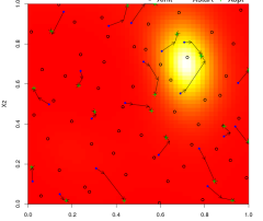
Figure 2 provides an illustrative view of this new capability by previewing the 2d toy example of Section 5. We started with a space-filling design ${\bar{\mathbf{X}}_{n}}$ in $[0,1]^{2}$, where 150 data points are evenly allocated on 50 unique design locations, shown as open circles. The true noise surface, $r(x)$, was derived from a standard bivariate Gaussian density with location $\mu=(0.7,0.7)$ and scale $\Sigma=0.02\cdot\mathbb{I}_{2}$. The heatmap depicts a HetGP-estimated standard deviation surface based on runs gathered at ${\bar{\mathbf{X}}_{n}}$. Higher noise regions are more yellow. We then set out to calculate coordinates of a new $M=20$ sized batch $\widetilde{\mathbf{X}}$ via IMSPE. Search is initialized with a LHS, shown in the figure as blue dots. Arrows originating from those dots show progress of the derivative-based search broken into three epochs for dramatic effect. Iterating to convergence requires hundreds of objective/gradient evaluations in the $Md=40$-dimensional search space, but these each take a fraction of a second because there are no large cubic operations. At the terminus of those arrows are green crosses, indicating the final locations of the new batch $\widetilde{\mathbf{X}}^{\star}$. Observe how some of these spread out relative to one another and to the open circles (mostly in the red, low-noise region), while others (especially near the yellow, high-noise region) are attracted to each other. At least one new replicate was found. Thus the IMSPE criterion strikes a balance between filling the space and creating replicates, which are good for separating signal from noise.

L-BFGS-B only guarantees a local minimum since the IMSPE objective is not a convex function. Actually, IMSPE surfaces become highly multi-modal as more points are added, with numbers of minima growing linearly in $n$, the number of unique existing design elements, even in the $M=1$ case. Larger batch sizes $M>1$ exacerbate this still further. There is also a “label-switching problem”. (Swap two elements of the batch and the IMSPE is the same.) To avoid seriously inferior local minima in our solutions for $\widetilde{\mathbf{X}}^{\star}$ we deploy a limited multi-start scheme, starting multiple L-BFGS-B routines simultaneously from novel sets of space-filling initial $\widetilde{\mathbf{X}}^{(0)}$, choosing the best at the end.

4 Hunting for replicates

Replication, meaning repeated simulations $Y(\mathbf{x})$ at fixed $\mathbf{x}$, keeps cubic costs down [Eqs. (3) and (7), reducing from $N$ to $n$] and plays an integral role in separating signal from noise (Ankenman et al.,, 2010; Binois et al.,, 2018b), a win-win for statistical and computational efficiency. Intuitively, replicates become desirable in otherwise poorly sampled high-variance regions (Binois et al.,, 2019). Unfortunately, a numerical scheme for optimizing IMSPE will never precisely yield replicates because tolerances on iterative convergence cannot be driven identically to zero. Consider again Figure 2, focusing now on the two new design points in the yellow region which went to similar final locations along their optimization paths. These look like potential replicates, but their coordinates don’t match.

One possible solution resolving near-replicates into actual ones is to introduce a secondary set of tolerances in the input space, whereby closeness implying “effective replication” can be deduced after the numerical solver finishes. This worked well for Binois et al., (2019), in part because of an additional replication-biased lookahead device (Ginsbourger and Le Riche,, 2010) Binois et al., used discrete search to check the degree to which future replicates could reduce IMSPE. But for us such tactics are unsatisfying on several fronts: lookahead isn’t manageable for $M\gg 1$ sized batches; additional input tolerances are tantamount to imposing a grid; such a scheme doesn’t directly utilize IMSPE information; and finally whereas one-at-a-time acquisition presents more opportunities to make adjustments in real-time, our batch setting puts more eggs in one basket. We therefore propose the following post-processing scheme on each batch which we call “backtracking”.

4.1 Backtracking via merge

For a new batch of size $M$, the possible number of new replicates ranges from zero to $M$. L-BFGS-B optimization yields $M$ unique coordinate tuples, but some may be very close to one another or the $n$ existing unique sites. Below we verbalize a simple greedy scheme for ordering and valuing those $M$ locations as potential “effective replicates”. Choosing among those alternatives happens in a second phase, described momentarily in Section 4.2.

Begin by recording the IMSPE of the solution $\widetilde{\mathbf{X}}_{M}\equiv\widetilde{\mathbf{X}}^{\star}$ provided by the optimizer: $I_{n+M}(\widetilde{\mathbf{X}}_{M})$. This corresponds to the no-backtrack/no-replicate option. Set iterator $s=0$ so that $\widetilde{\mathbf{X}}_{m_{s}}$ refers to this potential batch with $m_{s}=M$ unique design elements and let $d_{s}=0$. Move to the first iteration, $s=1$. Among the $m_{s-1}$ unique sites in $\widetilde{\mathbf{X}}_{m_{s-1}}$, find the one which has the smallest minimum distance $d_{s}$ to other unique elements in $\widetilde{\mathbf{X}}_{m_{s-1}}$ and existing sites ${\bar{\mathbf{X}}_{n}}$, with ties broken arbitrarily. Entertain a new batch $\widetilde{\mathbf{X}}_{m_{s}}$ by merging sights involved in that minimum $d_{s}$-distance pair. If both are a member of the new batch $\widetilde{\mathbf{X}}_{m_{s-1}}$, then choose a midway value for their new setting(s) in $\widetilde{\mathbf{X}}_{m_{s}}$. Otherwise, take the location from the existing (immovable) unique design element from ${\bar{\mathbf{X}}_{n}}$. Both imply $m_{s}=M-s$. Calculate $I_{n+m_{s}}(\widetilde{\mathbf{X}}_{m_{s}})$. Increment $s\leftarrow s+1$ and repeat unless $s=M$.

Figure 3: Left: backtracking with merge; gray arrows connect optimal $\widetilde{\mathbf{X}}_{m_{s}}$ with numbers indicating $s=1,\dots,M$; Right: IMSPE changes over numbers of replicates. Merging steps that are finally taken are shown in blue. Fitted segmented regression lines are overlaid.

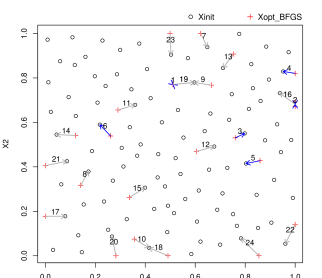
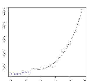
Figure 3 provides an illustration; settings of $f(\mathbf{x})$ and $r(\mathbf{x})$ mirror Figure 2. The existing design ${\bar{\mathbf{X}}_{n}}$ has $n=100$ unique elements, shown as open circles in the left panel. Each run is replicated three times so that $N=300$. A new batch of size $M=24$ is sought. Red crosses represent optimized $\widetilde{\mathbf{X}}_{m_{0}}=\widetilde{\mathbf{X}}_{M}$ from L-BFGS-B. Numbered arrows mark each backtracking step. Observe that the first two of these (almost on top of one another near the right-hand boundary) involve novel batch elements, whereas all others involve one of the $n$ existing sites. Aesthetically, the first five or so look reasonable, being nearby the high variance (top-right) region. Replication is essential in high-variance settings.

4.2 Selecting among backtracked batches

To quantify and ultimately automate that eyeball judgment, we investigated $I_{n+m_{s}}(\widetilde{\mathbf{X}}_{m_{s}})$ versus $s$, the number of replicates in the new batch. The right panel of Figure 3 shows the pattern corresponding to the backtracking steps on the left. Here, the sequence of $I_{n+m_{s}}(\widetilde{\mathbf{X}}_{m_{s}})$ values is mostly flat for $s=0,\dots,3$, then increasing thereafter. We wish to minimize IMSPE, except perhaps preferring exact replicates when IMSPEs may technically differ but are very similar. Aesthetically, that “change point” happens at $s=7$ where IMSPE jumps into a new and higher regime.

To operationalize that observation we experimented with a number of change point detection schemes. For example, we tried the tgp (Gramacy,, 2007; Gramacy and Taddy,, 2010) family of Bayesian treed constant, linear, and GP models. This worked great, but was overkill computationally. We also considered placing $d_{s}$, the minimizing backtracked pairwise distances, on the $x$-axis rather than $s$-values. Although the behavior with this choice was distinct, it yielded more-or-less equivalent selection on broad terms.

We ultimately settled on the following custom scheme recognizing that the left-hand regime was usually constant (i.e., almost flat), and the right-hand regime was generally increasing. To find the point of shift between those two regimes, we fit $M+1$ two-segment polynomial regression models, with break points $s=0,\dots,M$ respectively, with the first regime (left) being of order zero (constant) and the second (right) being of order four. We then chose as the location $\hat{s}$ the one whose two fits provide lowest in-sample MSE. The optimal pair of polynomial fit pairs are overlaid on the right panel of Figure 3, with groups color-coded to match arrows in the left panel.

Figure 4: Three selected scatter plots of IMSPE versus number of replicates with best change-point fitted regression lines overlaid. Colors match arrows in Figure 3.

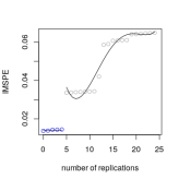
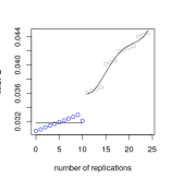
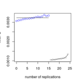
Figure 4 shows four other examples under the same broad settings but different random initial $n$-sized designs. The situation in the left panel matches that of Figure 3 and is by far the most common. The 2^nd panel depicts a setting where zero replicates is best but the two-regression scheme nevertheless identifies a midway change-point suggesting a bias toward finding at least some replicates. The 3^rd panel shows the case where no replicates are included. The right panel indicates an uncommon, opposite extreme. Note the small range of the IMSPE axis ($y$-axis). When the right-hand regime has uniformly lower IMSPE than the left-hand one, as may happen if merging identifies another local optima, we take $\hat{s}$ as the choice minimizing IMSPE in the right-hand regime.

5 Benchmarking examples

Here we illustrate and evaluate our method on an array of test problems. We have four examples total. Two are relegated to Appendix B: one mirroring the 1d example from Binois et al., (2019); another involves a 4d ocean simulator from McKeague et al., (2005). The other two, showcased here, include a 2d toy problem and an 8d “real simulator” from inventory management. Metrics include out-of-sample root mean-squared prediction error (RMSPE), i.e., matching our IMSPE acquisition heuristic, and a proper scoring rule (Gneiting and Raftery,, 2007, Eq. (27)) combining mean and uncertainty quantification accuracy, which for GPs reduces to predictive log likelihood. We also consider computing time and number of unique design elements, $n$, over total acquisitions $N$. Our gold standard benchmark is the “pure sequential” ($M=1$) adaptive lookahead scheme of Binois et al.,, however when relevant we also showcase other special cases. Our goal is not to beat that benchmark. Rather we aim to be competitive while entertaining $M=24$-sized batches, representing the number of cores on a single supercomputing node.

5.1 2d toy example

Elements of this example have been in play in previous illustrations, including Figures 2–3. The true mean function $f(\mathbf{x})$ is defined as:

$$f(\mathbf{x})=f(x_{1},x_{2})=20\left[\frac{a_{1}}{\exp(a_{1}^{2}+a_{2}^{2})}+\frac{a_{3}}{\exp(a_{3}^{2}+a_{4}^{2})}\right],$$

where $a_{1}=6x_{1}-4.1$, $a_{2}=6x_{2}-4.1$, $a_{3}=6x_{1}-1.7$, and $a_{4}=6x_{2}-1.7$. The true noise surface, $r(\mathbf{x})$, is a bivariate Gaussian density with location $\mu=(0.7,0.7)$ and scale $\Sigma=0.02\cdot\mathbb{I}_{2}$. Figure 5 provides a visual using color for $f(\mathbf{x})$ and contours for $r(\mathbf{x})$. We deliberately made the mean surface have the same signal structure at the bottom left and top right regions. However, the top right region is exposed to high noise intensity while the bottom left region is almost noise-free, creating distinct signal-to-noise regimes.

Figure 5: The heatmap shows the mean surface $f(\mathbf{x})$. Lighter colors correspond to higher values. Contours of $r(\mathbf{x})$ are overlaid.

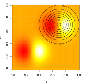
Design aspects of our experiment(s) were set up as follows. We begin with an $n_{0}=20$-sized maximin–LHS with five replicates upon each for $N_{0}=100$ total simulations. This is followed by ten batches of IMSPE-acquisition with backtracking for 240 new runs ($N=340$ total).

Figure 6: IMSPE design in batches: gray dots are initial design points; gray contours show signal and noise contrast; numbers indicate replicate multiplicity. The last two panels summarize all new points from 6 batches and all design points respectively.

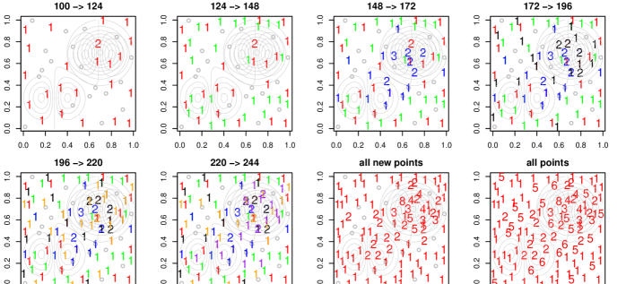
Figure 6 shows how the first six batches distributed in the input space, with one panel for each. Color is used to track batches over accumulated runs; numbers indicate degrees of replication. For example, the first batch had two replicates (one at a unique input, one at an existing open circle), whereas the third batch had many more. Observe that as batches progress, more replicates and more unique locations cluster near the noisy top-right region of the input space. The final two panels summarize all (new) points involved in those first six batches, including the initial design.

Figure 7: Results of RMSPE, score, time per iteration in fitting hetGP model, and the aggregate number of unique design locations from 50 MC repetitions.

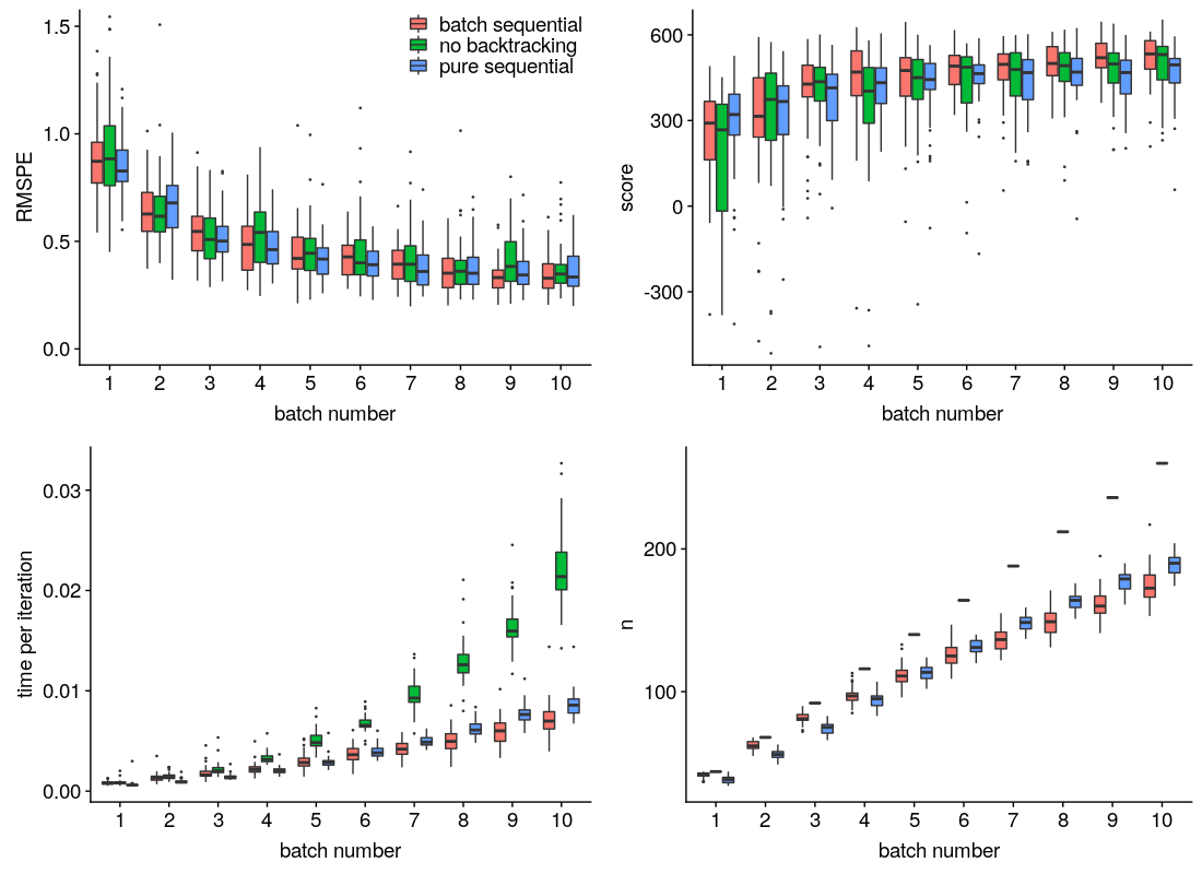
Figure 7 offers a comparison to Binois et al., (2019)’s pure sequential ($M=1$) strategy in a fifty-repetition MC exercise. Randomization is over the initial maximin–LHS, noise deviates in simulating the response, and novel LHS testing designs of size $N=500$. We also include a “no backtracking” comparator, omitting the search for replicates step(s) described in Section 4. For the pure sequential benchmark, we calculate RMSPE and score after every 24 subsequent steps to make it comparable to our batches. In terms of RMSPE, all three methods perform about the same. Under the other three metrics, batch-with-backtracking is consistently better than the non-backtracking version: more replicates, faster HetGP fits due to smaller $n$, and higher score after batch three. The degree of replication yielded by backtracking is even greater than the pure sequential scheme after batch four. Also from batch four, batch IMSPE outperforms pure sequential design on score.

5.2 Assemble-to-order

The assemble-to-order (ATO) problem (Hong and Nelson,, 2006) involves a queuing simulation targeting inventory management scenarios. It was designed to help determine optimal inventory levels for eight different items to maximize profit. Here we simply treat it as blackbox response surface. Although the signal-to-noise ratio is relatively high, ATO simulations are known to be heteroskedastic (Binois et al.,, 2018b). We utilized the MATLAB implementation described by Xie et al., (2012) through R.matlab (Bengtsson,, 2018) in R. Our setup duplicates the MC of Binois et al., (2019) in thirty replicates, in particular by initializing with a $n_{0}=100$-sized random design in the 8d input space, paired with random degrees of replication $a_{i}\sim\mathrm{Unif}\{1,\dots,10\}$ so that the initial design comprised about $N_{0}\approx 500$ runs. Binois et al., then performed about 1500 acquisitions to end at $N=2000$ total runs. We performed sixty-three $M=24$-sized batches to obtain about 2012 runs.

Since the 8d inventory input vector must be comprised of integers $\{0,\dots,20\}$, we slightly modified our method in a manner similar to Binois et al.,: inputs are coded to $[0,1]$ so that IMSPE optimization transpires in an $M\times[0,1]^{8}$ space. When backtracking, merged IMSPEs are calculated via rounded $\widetilde{\mathbf{X}}_{m_{s}}^{\mathrm{int}}$ on the natural scale.

Figure 8: RMSPE and score over design size $N$ from 30 MC repetitions.

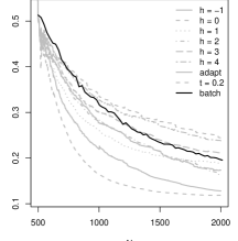
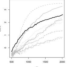
Figure 8 shows progress in terms of average RMSPE and score mimicking the format of the presentation of Binois et al.,, whose comparators are duplicated in gray in our updated version. There are eight gray variations, representing multiple lookahead horizons ($h$) and two automated horizon alternatives, with “Adapt” being the gold standard. In terms of RMSPE, our batch method makes progress more slowly at first, but ultimately ends in the middle of the pack of these pure sequential alternatives. In terms of score, we start out the best, but end in the third position. Apparently, our batch scheme is less aggressive on reducing out-of-sample mean-squared error, but better at accurately assessing uncertainty. In the 30 MC instances our average number of new replicates per unique site was 1.64 (min 0, max 5), leading to a mean of $n=1610$ (min 1606, max 1612). This is a little higher (lower replication) than $n=1086$ (min 465, max 1211) reported by Binois et al., for “Adapt”. Again, we conclude that our batch method is competitive despite being faced with many fewer opportunities to re-tune the strategy over acquisition iterations.

6 Delta smelt

Encouraged by these results, and by simulations in Section 5, we return now our motivating delta smelt ABM application. Time and allocation limits meant only one crack at this, so we did one last “sanity check”, extending the pilot study with batch acquisitions, before embarking on a big batch-sequential simulation campaign. This analysis, which was also encouraging, is described in detail in Appendix C.

6.1 Setup and acquisitions

For our“full” simulation campaign and analysis of the delta smelt ABM where we explored a ten-dimensional input space on a 7d manifold. See Table 2, augmenting Table 1 with a new column. This analysis expanded the effective input domain by three, and involved slightly adjusted ranges and relationships between the original inputs. Specifically, we extended $m_{y}$ and began to vary $P_{l,2}$, $P_{a,3}$, and $P_{a,4}$ with dependencies $P_{p,6}=P_{p,2}\times 1.75+0.05$, $P_{j,3}=P_{j,6}$, and $P_{a,3}=P_{a,4}$. Inputs $m_{l}$, $m_{p}$, and $m_{a}$ remain fixed at their default values.

symbol	range	default	pilot study	full study
$m_{y}$	[0.01,0.50]	0.035	0.035	[0.02, 0.05]
$m_{l}$	[0.01, 0.08]	0.050	0.050	0.050
$m_{p}$	[0.005, 0.05]	0.030	0.030	0.030
$m_{j}$	[0.001, 0.025]	0.015	[0.005,0.030]	[0.005, 0.030]
$m_{a}$	[0.001, 0.01]	0.006	0.006	0.006
$m_{r}$	[0.005, 0.05]	0.020	[0, 0.05]	[0, 0.1]
$P_{l,2}$	[0.10, 20.0]	0.200	0.200	[0.1, 0.5]
$P_{p,2}$	[0.10, 20.0]	0.800	[0.10, 1.84]	[0.10, 1.84]
$P_{p,6}$	[0.10, 20.0]	1.500	$P_{p,2}$	1.75$P_{p,2}+0.05$
$P_{j,3}$	[0.10, 20.0]	0.600	[0.1, 1.5]	[0.1, 1.5]
$P_{j,6}$	[0.10, 20.0]	0.600	$P_{j,3}$	$P_{j,3}$
$P_{a,3}$	[0.01, 20.0]	0.070	0.070	[0.05, 0.15]
$P_{a,4}$	[0.01, 5.0]	0.070	0.070	$P_{a,3}$

Table 2: Augmenting Table 1 to show the parameter settings of the “full” experiment.

To explore the 7d input space, we begin with maximin-LHS of size $n_{0}=192$, each with five replicates for a total of $N_{0}=960$ initial runs. We aim to more than double this simulation effort, collecting a total of $N=2016$ runs, by adding 44 subsequent batches of size $M=24$. This took a total of 50 days, requiring slightly more than one day per batch, including HetGP updates, IMSPE evaluation and backtracking, and any time spent waiting in the queue on the ARC HPC facility at Virginia Tech. Inevitably, some hiccups prevented a fully autonomous scheme. In at least one case, what seemed to be a conservative request of 10 hours of job time per batch (of runs that usually take 4-6 hours) was insufficient. We had to manually re-run those failed simulations, and subsequently upped requests to 14 hours. This bigger demand led to longer queuing times even though the average execute time was at par with previous campaigns.

When training the HetGP surrogate we used responses $y_{i}=\log\lambda_{i}$ for nonzero simulation outputs. Any zeros are replaced with $y_{i}=\log\frac{1}{2}\min_{\{i:\lambda_{i}>0\}}\lambda_{i}$ where $\{i:\lambda_{i}>0\}$ represents the subset of $\{1,\dots,N\}$ indexing positive outputs. This lead to slightly different $y$-axis scales for visuals compared to Section 2.3. An adaptive scheme for handling zeros was necessitated by the dynamic nature of the arrival of $\lambda$-values furnished over the batches of sequential acquisition – in particular of ones smaller than those obtained in the pilot study.

mean surface	variance surface	1d predictive bands

Figure 9: Slices for the “full” experiment, updating Figure 1. The horizontal gray line in the right column indicates $y=\log\frac{1}{2}\min_{\{i:\lambda_{i}>0\}}\lambda_{i}$, the value assigned to extinction outputs.

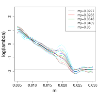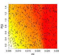
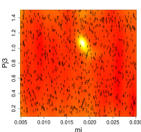
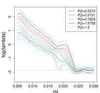
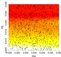
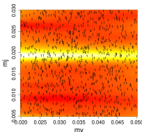
To illustrate, see Figure 9 which augments mean and standard deviation slice views first provided in Figure 1. Here, to reduce clutter, numbers overlaid indicate the degrees of replication on only the batch/IMSPE selections. As before, these are projections over the other five dimensions, so the connection between variance and design multiplicity is weak (obfuscating how uncertainty relates to the other five inputs). Nevertheless, multiplicity in unique runs is generally higher (more 4s–6s) in the yellow regions. The first row of Figure 9 coincides with Figure 1, showing input pair $m_{j}\times P_{j,3}$. Observe that, after conditioning on more data despite the larger space, predictive bands over $m_{j}$ are narrower, especially at the boundaries. The sudden widening of the dark blue predictive intervals correspond to the yellow spot in the middle panel. The second row shows a newly selected pair $m_{y}\times m_{j}$, replacing the flat view from Figure 1 which is still uninteresting in the “full” setting. A nonlinear variance is evident, being highest near $m_{j}=0.020$.

6.2 Downstream analysis

Slices are certainly not the best way to visualize a high dimensional response surface. Moreover, there are many possible ways to utilize the information in a fitted surrogate. Our intent here is not to explore that vast space in any systematic way, but rather to illustrate potential. Here we showcase input sensitivity analysis as one possible task downstream of fitting and design. That is, we seek to determine which input variables have the greatest influence on outputs, i.e., the growth rate of the fish in this example, and which variables (if any) interact to affect changes in the response. We perform this analysis based exclusively on the $N=2016$ runs obtained from the batch sequential design experiment. We could have combined with the pilot runs, which may have reduced variability in some parts of the input space, but could potentially introduce complications interpretively.

Sensitivity analysis for GP surrogates (Oakley and O’Hagan,, 2004; Marrel et al.,, 2009) attempts to measure the effect of a subset of inputs on outputs by controlling and averaging over the compliment of inputs (Saltelli et al.,, 2000). In this way, one can furnish a meaningful low-dimensional summary of inherently high-dimensional relationships. Gramacy, (2020), Chapter 8.2, provides a thorough summary alongside a portable implementation. We briefly summarize salient details here for completeness.

Let $U(\mathbf{x})=\prod_{k=1}^{m}u_{k}(x_{k})$ denote a distribution on inputs, indicating relative importance in the range of settings or nearby nominal values. We take $U$ as uniform over the study region in Table 2. So-called main effects, sometimes referred to as a zeroth-order index, are calculated by varying one input variable while integrating out others under $U$:

$$\mathrm{ME}(x_{j})\equiv\mathbb{E}_{U_{-j}}\{y\mid x_{j}\}=\int\!\!\int_{\mathcal{X}_{-j}}\!yP(y\mid\mathbf{x})u_{-j}(x_{1},x_{j-1},x_{j+1},x_{m})\,d\mathbf{x}_{-j}dy.$$ (9)

Above, $P(y\mid\mathbf{x})=P(Y(\mathbf{x})=y)$ is the predictive distribution from a surrogate, $\hat{f}$ say via HetGP. One may approximate this double-integral via MC with LHSs over $U$. We used LHSs of size 10000 paired with a common grid over each variable $j$ involved in $\mathrm{ME}(x_{j})$.

The top-left of Figure 10 reveals that all inputs show a negative relationship with the response $\lambda$, with greater values leading to declining populations. Apparently, $m_{j}$ and $P_{j,3}$ induce higher mean variation in the response than the others. These results indicate that juvenile mortality ($m_{j}$) and the feeding parameter for juvenile food type 3 ($P_{j,3}$) have the greatest impact on the mean value of the response (Figure 10, top row). Further, $m_{j}$ exhibits a thresholding effect – above a value of about 0.025 the simulated population almost always goes extinct within the time frame of the simulation (Figure 9, right panels). However, when $m_{j}$ takes on values between 0.018 and 0.022, or so, uncertainty in the estimate of mean behavior increases substantially. This due to the individuals comprising the population becoming low in abundance and smaller in size to the point that egg production cannot offset lifetime mortality.

As we mentioned in Section 2.2, HetGP puts a second GP prior on the latent nuggets $\boldsymbol{\Delta}_{n}$. Once $\boldsymbol{\Delta}_{n}$ and all hyperparameters are estimated, the predictive mean of the noise process, i.e., the smoothed nuggets $\boldsymbol{\Lambda}$, can be calculated over any testing data set in the domain of interest. This provides a way to assess the influence of each input variable on the heteroskedastic variance. Applying the same procedures as above, main effects for the noise process are produced in the bottom-left of Figure 10. Observe that when $m_{j}$ is between 0.4 and 0.6 variance effects are highest, particularly for $m_{j}$ and $P_{j,3}$. As far as we know, such main effects (and higher-order sensitivities) on variances are novel in the literature.

Figure 10: Sensitivity analysis for mean (top) and variance process (bottom): main effects (left); first order (middle) and total sensitivity (right) from 100 bootstrap re-samples.

To further quantify the variation that each input factor contributes, we calculated first-order ($S$) and total ($T$) indices. These assume a functional ANOVA decomposition,

$$f(x_{1},\dots,x_{m})=f_{0}+\sum_{j=1}^{m}f_{j}(x_{j})+\!\!\sum_{1\leq i<j\leq m}f_{ij}(x_{i},x_{j})+\cdots+f_{1,\dots,m}(x_{1},\dots,x_{m}),$$

so that $$\mathbb{V}\mathrm{ar}_{U}(y\mid x_{1},\dots,x_{m})=\sum_{j=1}^{m}V_{j}+\!\!\sum_{1\leq i<j\leq m}V_{ij}+\cdots+V_{1,\dots,m},$$

where $V_{j}=\mathbb{V}\mathrm{ar}_{U_{j}}(\mathbb{E}_{U_{-j}}\{y\mid x_{j}\})$, $V_{ij}=\mathbb{V}\mathrm{ar}_{U_{ij}}(\mathbb{E}_{U_{-ij}}\{y\mid x_{i},x_{j}\})-V_{i}-V_{j}$. In a direct application, $f$ above is the simulator. Since that is expensive in our delta smelt case, we use the surrogate $\hat{f}$ instead. The second equation decomposes, and quantifies, variability in $\mathbb{E}_{U_{J}}\{y\mid\mathbf{x}_{J}\}$ with respect to changes in $\mathbf{x}_{J}$ according to $U_{J}(\mathbf{x}_{J})$. It holds for our HetGP $\hat{f}$ since all input factors can be varied independently in the input hypercube. First-order sensitivity $S_{j}$ for $x_{j}$ measures the proportion of variation that $x_{j}$ contributes to the total:

$$S_{j}=\frac{\mathbb{V}\mathrm{ar}_{U_{j}}(\mathbb{E}_{U_{-j}}\{y\mid x_{j}\})}{\mathbb{V}\mathrm{ar}_{U}(y)},\quad j=1,\dots,m.$$

Total sensitivity $T_{j}$ is the mirror image:

$$T_{j}=\frac{\mathbb{E}\{\mathbb{V}\mathrm{ar}(y\mid\mathbf{x}_{-j})\}}{\mathbb{V}\mathrm{ar}(y)}=1-\frac{\mathbb{V}\mathrm{ar}(\mathbb{E}\{y\mid\mathbf{x}_{-j}\})}{\mathbb{V}\mathrm{ar}(y)}.$$

It considers the proportion of variability that is not explained without $x_{j}$. The difference between first-order and total sensitivities, i.e., $T_{j}-S_{j}$, may be taken as a measure of variability in $y$ due to the interaction between input $j$ and the other inputs.

With HetGP surrogate $\hat{f}$ for $y\mid\mathbf{x}$, calculation of $S$ and $T$ indices may also be undertaken by MC via LHS. The details are omitted here for brevity. We repeated MC calculations of both on 100 bootstrap samples of the original data set. A summary via boxplots is provided in the right panels of Figure 10. These views match the main effects: $m_{j}$ and $P_{j,3}$ stand out in both plots. First-order sensitivity ($S$) for the variance (bottom-middle), fails to flag an obvious difference between variables. Via total sensitivity ($T$, bottom-right), indices for $m_{j}$ and $P_{j,3}$ are again apparently higher than other variables, suggesting that a substantial aspect of the effect of these variables on variability is through interactions.

Proportion	$m_{y}$	$m_{j}$	$m_{r}$	$P_{l,2}$	$P_{p,2}$	$P_{j,3}$	$P_{a,3}$
Main process	0.54	1	0.66	0.68	0.53	1	0.55
Noise process	0.74	0.99	0.92	0.80	0.75	0.97	0.80

Table 3: Proportion of positive $I=T-S$ indices.

Using those $S$ and $T$ values, we computed $I=T-S$. As Saltelli et al., (2000) describes, this quantity $I$ is positive if variability in the response can be attributed to interactions between inputs. The proportion of our bootstrapped $I$ measurements which are positive is provided in Table 3. Again, $m_{j}$ and $P_{j,3}$ flag has highly probable for impacting the response through an interaction with other variables. Input $P_{l,2}$ may also have substantial impact on $\lambda$ through interactions. Input $m_{r}$ has the third highest measurement. In fact, all of the variables suggest statistically noteworthy affect through interaction by comparison to the so-called median probability model (Barbieri et al.,, 2004) implied by a $p=0.5$ threshold. Since not many variables contribute via zeroth (main effect) and first-order summaries, it is perhaps not surprising that action is exposed through interaction.

The results of this analysis reveal that although juvenile mortality is important for the overall mean, it by itself does not determine whether a population will increase or decrease (i.e., $\lambda>0$ or $<0$). For example, although it will typically be important for the average value of $m_{j}$ to be below 0.015 or so, the average value of $\lambda$ will depend, sometimes sensitively, on the values of other parameters (Figure 9, top right panel), or through their interactions (Table 3). The complex nature of these sensitivities implies that environmental variation and management actions that affect these key parameters will likely generate non-linear responses in population growth rate that depend on the interactive effects among parameters. In addition, several parameters (e.g., $m_{r}$) have important effects on the variance of population growth rate, further complicating any assessment of the value of an individual parameter. Predicted population responses to actions directed at affecting change in specific biological processes (e.g., mortality rate of juveniles, $m_{j}$) should be viewed in the context of the state of the system and population. Simple changes to key parameters will likely not lead to simple responses (i.e., change in magnitude and variance of growth rate) but rather to ones that depend on the values of other parameters.

More importantly than the specific predictions, however, the analysis allows us to characterize the emergent behavior of this complex simulation model. The goal of ABMs is to incorporate possible mechanisms that are believed to impact dynamics of complex systems. However model builders cannot typically predict, a priori, the full dynamics of the model across all possible parameter settings. An appropriately designed surrogate allows us to quickly probe the model more deeply without needing to re-run the full simulation at every parameter combination of interest, potentially at enormous computational expense. For example, by independently varying input factors, we are able to compare their relative contribution and investigate higher-order interactions without new runs of the simulator. Further, once dominant variables are identified, fixing them can unravel the sensitivities of the remaining variables. As one further example, we fixed $m_{j}$ and $P_{j,3}$ and made an analogue of Figure 10 over the other five factors. See Appendix D for details.

7 Discussion

Motivated by a computationally intensive stochastic agent-based model simulating the ecosystem and life cycles of delta smelt, an endangered fish, we developed a batch sequential design scheme for loading supercomputing nodes with runs in batches. We used a heteroskedastic Gaussian process (HetGP) surrogate to acknowledge nonlinear dynamics in mean and variance, revealed in a limited pilot study, and extended a variance-based (IMSPE) scheme for sequential design under such models to allow the selection of multiple new runs at once. To facilitate numerical optimization of batch IMSPE we furnished closed form derivatives and developed a backtracking scheme to determine if any near replicates provided by the solver were better as actual replicates. Only actual replicates efficiently separate signal from noise and pay computational dividends at the same time.

Our methods were illustrated and contrasted against previous (pure sequential/one-at-a-time) active learning strategies on several synthetic and real-simulation benchmarks. These allowed us to conclude that our scheme was no worse than previous approaches, while designing batches of runs that could fill out a supercomputing node. Since those one-at-a-time schemes already outperformed single-batch designs, we conclude by proxy that ours do as well, and verified as much in additional experimentation (not provided). We then turned to our motivating delta smelt scenario to undertake a simulation campaign with thousands of runs in an expanded domain. Those simulations required 12000 core hours, which would have spanned more than 500 days if run back-to-back (and not counting any queue delays). Instead the batch campaign, took us about 55 days to run (including substantial queuing).

This order of magnitude reduction in “scientist time”, without noticeable drawbacks in modeling efficiency, could have a substantial impact on the modus operandi of conducting stochastic simulation experiments in practice. Widespread university and research lab access to supercomputing facilities is democratizing the application of mathematical modeling of complex physical and biological phenomena. However, strategies for planning those experiments in this unique architectural environment are sorely needed. We think the advances reported on here take an important first step. Simulations in hand, there are many interesting analyses which can be performed downstream. We provided some visuals based on slices and performed an input sensitivity analysis in order to determine which factors have the largest effect on smelt mortality in this particular system. Our choice of IMSPE suits this analysis well because it reduces variance globally and our Saltelli-style indices emphasize decomposition of variance. Extending Binois et al.,’s IMSPE calculation to other downstream tasks has become a cottage industry of late. Examples include sequential learning of active subspaces (Wycoff et al.,, 2019), level-set finding and Bayesian optimization (Lyu et al.,, 2018). Cole et al., (2020) adapt a similar calculation for large-scale local GP approximation via inducing points. We see no barriers to extending these schemes similarly, to batch analogs of one-at-a-time acquisitions. Kennedy and O’Hagan, (2001)-style calibration of stochastic simulators remains on the frontier of design for surrogate modeling. Baker et al., (2020) identify this as an important area for further research.

One might wonder if a Binois-like one-at-a-time scheme could be adapted for batch acquisition by inserting “synthetic data”, obtained from the predictive distribution, for earlier (waiting to run) selections while entertaining the selection of latter batch elements. Although there are many ways to operationalize such an idea, we think this is flawed for several reasons. One is that the high and changing noise scenario would demand entertaining large numbers of replicates for those synthetic data, eliminating any computational advantage. We found this too prohibitive to entertain as a comparator. Another is that such a scheme would be unnecessarily making a greedy approximation to a joint optimization. Although joint derivatives are much more work to derive, they are simple to code now that we have provided them. No greedy approximation is necessary.

There is certainly potential for improving our scheme. We took a geometric mean to get scalar output for smelt simulations. Analyzing higher-dimensional outputs could reveal additional nuance, however HetGP surrogate modeling for such settings remains on the frontier. The performance of our scheme relies heavily on local numerical optimization via libraries. Finding global optima for non-convex criteria in high-dimensional spaces is always a challenge. Although we get good results with L-BFGS-B, we also tried particle swarm optimization (PSO; Kennedy and Eberhart,, 1995) in several capacities: replacing BFGS wholesale and for finding good BFGS staring points. Improvements were consistent but minor in the grand scheme of multiple batches of sequential design. We believe that other gradient-free/coordinate exchange methods would perform similarly. Hybrid genetic and gradient-based optimization (Mebane and Sekhon,, 2011) could be promising, as could a weighted least-squares approach to identifying candidate numbers of replicates (Li and Deng,, 2018). Trade-offs between queue time and batch size might be worth exploring, however that could be a fractal undertaking: a meta computer experiment would be needed to map out the response surface of run/wait times based on run configuration and other (computing) environment variables. We kept it simple with $M=24$ to match the number of cores on the compute nodes, as advised by the VT ARC office. Another option is unknown batch sizes or on-demand acquisition: whenever a batch of cores is available the model/design scheme must be ready to furnish runs. This could be accomplished by maintaining a larger $M$-sized queue of prioritized inputs, say following Gramacy and Lee, (2009), which would need to be updated for the HetGP framework.

Focusing on the delta smelt ABM in particular, the current version of the simulator makes several fundamental assumptions that influence the population dynamics and can affect measured input sensitivities. Future analysis could accommodate additional parameters, such as those related to juvenile and adult movement behaviors that affect their growth and mortality. One could also address structural uncertainty in the delta smelt ABM. For example, movement rates are held constant for all individuals within each life stage and maturity is a fixed threshold function of length. Rose et al., (2013b) examined alternative setups to assess how different assumptions would affect model results. They formulated mortality to continuously decrease with length, to be density-dependent (rather than constant), and substituted a smoothed function of maturity-by-length for the threshold, and repeated the ten year simulations. A future simulation campaign (perhaps using the same parameters selected for the analysis reported here or under a novel batch-sequential design) repeated under these alternative assumptions would provide valuable additional information on model sensitivities and uncertainties.

Acknowledgments

Authors BZ and RBG gratefully acknowledge funding from a DOE LAB 17-1697 via subaward from Argonne National Laboratory for SciDAC/DOE Office of Science ASCR and High Energy Physics. RBG recognizes partial support from National Science Foundation (NSF) grant DMS-1821258. LRJ recognizes partial support from NSF grant DMS/DEB-1750113. We also gratefully acknowledge computing support from Virginia Tech’s Advanced Research Computing (ARC) facility. We thank Xinwei Deng, Dave Higdon and Leanna House (Virginia Tech) for valuable insights and suggestions.

Appendix A IMSPE gradient

Omitted expressions for the IMSPE gradient in Section 3.2 are provided below.

$$\dfrac{\partial\mathbf{K}^{-1}_{n+M}}{\partial\tilde{\mathbf{x}}_{i(p)}} =\dfrac{\partial}{\partial\tilde{\mathbf{x}}_{i(p)}}\begin{bmatrix}\mathbf{K}_{n}^{-1}+g(\widetilde{\mathbf{X}})\Sigma(\widetilde{\mathbf{X}})g(\widetilde{\mathbf{X}})^{\top}&g(\widetilde{\mathbf{X}})\\ g(\widetilde{\mathbf{X}})^{\top}&\Sigma(\widetilde{\mathbf{X}})^{-1}\end{bmatrix}=\begin{bmatrix}H(\widetilde{\mathbf{X}})&Q(\widetilde{\mathbf{X}})\\ Q(\widetilde{\mathbf{X}})^{\top}&V(\widetilde{\mathbf{X}})\end{bmatrix}\quad,$$

$$\mbox{where}\;\;V(\widetilde{\mathbf{X}}) :=-\Sigma(\widetilde{\mathbf{X}})^{-1}\frac{\partial\Sigma(\widetilde{\mathbf{X}})}{\partial\tilde{\mathbf{x}}_{i(p)}}\Sigma(\widetilde{\mathbf{X}})^{-1}$$

$$Q(\widetilde{\mathbf{X}}) :=\dfrac{\partial g(\widetilde{\mathbf{X}})}{\partial\tilde{\mathbf{x}}_{i(p)}}=-\mathbf{K}_{n}^{-1}\left(c({\bar{\mathbf{X}}_{n}},\widetilde{\mathbf{X}})V(\widetilde{\mathbf{X}})+{\color[rgb]{0,0,0}\frac{\partial c({\bar{\mathbf{X}}_{n}},\widetilde{\mathbf{X}})}{\partial\tilde{\mathbf{x}}_{i(p)}}}\Sigma(\widetilde{\mathbf{X}})^{-1}\right)$$

$$H(\widetilde{\mathbf{X}}) :=\dfrac{\partial g(\widetilde{\mathbf{X}})\Sigma(\widetilde{\mathbf{X}})g(\widetilde{\mathbf{X}})^{\top}}{\partial\tilde{\mathbf{x}}_{i(p)}}$$

$$=g(\widetilde{\mathbf{X}})\dfrac{\partial\Sigma(\widetilde{\mathbf{X}})}{\partial\tilde{\mathbf{x}}_{i(p)}}g(\widetilde{\mathbf{X}})^{\top}\!+\!Q(\widetilde{\mathbf{X}})\Sigma(\widetilde{\mathbf{X}})g(\widetilde{\mathbf{X}})^{\top}\!+\!\{Q(\widetilde{\mathbf{X}})\Sigma(\widetilde{\mathbf{X}})g(\widetilde{\mathbf{X}})^{\top}\}^{\top}.$$

Recall that $\Sigma(\widetilde{\mathbf{X}})=r(\widetilde{\mathbf{X}})+c(\widetilde{\mathbf{X}},\widetilde{\mathbf{X}})-c({\bar{\mathbf{X}}_{n}},\widetilde{\mathbf{X}})^{\top}\mathbf{K}_{n}^{-1}c({\bar{\mathbf{X}}_{n}},\widetilde{\mathbf{X}})$. Again recursing with the chain rule, first diagonal matrix $r(\widetilde{\mathbf{X}})$ via Eq. (2), gives

$$\frac{\partial r(\widetilde{\mathbf{X}})}{\partial\tilde{\mathbf{x}}_{i(p)}}=\frac{\partial{\color[rgb]{0,0,0}c}_{(\boldsymbol{\delta})}(\widetilde{\mathbf{X}},{\bar{\mathbf{X}}_{n}})}{\partial\tilde{\mathbf{x}}_{i(p)}}(\mathbf{C_{(\boldsymbol{\delta})}}+g_{(\boldsymbol{\delta})}\mathbf{A}^{-1})^{-1}\boldsymbol{\Delta}_{n}.$$ (10)

It is worth observing here how relative noise levels, smoothed through $\boldsymbol{\Delta}_{n}$ and distance to ${\bar{\mathbf{X}}_{n}}$, impact the potential value of new design elements $\widetilde{\mathbf{X}}$. High variance $\bar{\mathbf{x}}_{i}$ have low impact unless $a_{i}$ is also large, in which case there is an attractive force encouraging replication (elements of $\widetilde{\mathbf{X}}$ nearby ${\bar{\mathbf{X}}_{n}}$). The last component of $\frac{\partial\Sigma(\widetilde{\mathbf{X}})}{\partial\tilde{\mathbf{x}}_{i(p)}}$ relies on $\frac{\partial c({\bar{\mathbf{X}}_{n}},\widetilde{\mathbf{X}})}{\partial\tilde{\mathbf{x}}_{i(p)}}$, a quadratic:

$$\frac{\partial}{\partial\tilde{\mathbf{x}}_{i(p)}} c({\bar{\mathbf{X}}_{n}},\widetilde{\mathbf{X}})^{\top}\mathbf{K}_{n}^{-1}c({\bar{\mathbf{X}}_{n}},\widetilde{\mathbf{X}})$$ (11)

$$=c({\bar{\mathbf{X}}_{n}},\widetilde{\mathbf{X}})^{\top}\mathbf{K}_{n}^{-1}\frac{\partial c({\bar{\mathbf{X}}_{n}},\widetilde{\mathbf{X}})}{\partial\tilde{\mathbf{x}}_{i(p)}}+\left\{c({\bar{\mathbf{X}}_{n}},\widetilde{\mathbf{X}})^{\top}\mathbf{K}_{n}^{-1}\frac{\partial c({\bar{\mathbf{X}}_{n}},\widetilde{\mathbf{X}})}{\partial\tilde{\mathbf{x}}_{i(p)}}\right\}^{\top}.$$

The structure of this component’s derivative reveals how new design elements $\widetilde{\mathbf{X}}$ repel one another and push away from existing points ${\bar{\mathbf{X}}_{n}}$. In other words, the forces described in Eqs. (10–11) trade-off in a sense, encouraging both spread to space-fill and compression toward replication depending on the noise level $r(\cdot)$.

The other terms that are included in $\frac{\partial\Sigma(\widetilde{\mathbf{X}})}{\partial\tilde{\mathbf{x}}_{i(p)}}$ are as follows:

$$\frac{\partial c({\bar{\mathbf{X}}_{n}},\widetilde{\mathbf{X}})}{\partial\tilde{\mathbf{x}}_{i(p)}} =\frac{\partial}{\partial\tilde{\mathbf{x}}_{i(p)}}\begin{bmatrix}c(\tilde{\mathbf{x}}_{1},\bar{\mathbf{x}}_{1})&\!\cdots\!&c(\tilde{\mathbf{x}}_{M},\bar{\mathbf{x}}_{1})\\ \vdots&&\vdots\\ c(\tilde{\mathbf{x}}_{1},\bar{\mathbf{x}}_{n})&\!\cdots\!&c(\tilde{\mathbf{x}}_{M},\bar{\mathbf{x}}_{n})\\ \end{bmatrix}=\begin{bmatrix}&\frac{\partial c(\tilde{\mathbf{x}}_{i},\bar{\mathbf{x}}_{1})}{\partial\tilde{\mathbf{x}}_{i(p)}}&\\ \mathbf{0}_{n\times(i-1)}&\vdots&\mathbf{0}_{n\times(M-i)}\\ &\frac{\partial c(\tilde{\mathbf{x}}_{i},\bar{\mathbf{x}}_{n})}{\partial\tilde{\mathbf{x}}_{i(p)}}&\\ \end{bmatrix}$$

$$\frac{\partial c(\widetilde{\mathbf{X}},\widetilde{\mathbf{X}})}{\partial\tilde{\mathbf{x}}_{i(p)}} =\frac{\partial}{\partial\tilde{\mathbf{x}}_{i(p)}}\begin{bmatrix}c(\tilde{\mathbf{x}}_{1},\tilde{\mathbf{x}}_{1})&\!\!\!\cdots\!\!\!&c(\tilde{\mathbf{x}}_{M},\tilde{\mathbf{x}}_{1})\\ \vdots&&\vdots\\ c(\tilde{\mathbf{x}}_{1},\tilde{\mathbf{x}}_{M})&\!\!\!\cdots\!\!\!&c(\tilde{\mathbf{x}}_{M},\tilde{\mathbf{x}}_{M})\\ \end{bmatrix}=\begin{bmatrix}&&\frac{\partial c(\tilde{\mathbf{x}}_{i},\tilde{\mathbf{x}}_{1})}{\partial\tilde{\mathbf{x}}_{i(p)}}&&\\ &&\vdots&&\\ \frac{\partial c(\tilde{\mathbf{x}}_{i},\tilde{\mathbf{x}}_{1})}{\partial\tilde{\mathbf{x}}_{i(p)}}&\!\!\cdots\!\!&\frac{\partial c(\tilde{\mathbf{x}}_{i},\tilde{\mathbf{x}}_{i})}{\partial\tilde{\mathbf{x}}_{i(p)}}&\!\!\cdots\!\!&\frac{\partial c(\tilde{\mathbf{x}}_{i},\tilde{\mathbf{x}}_{M})}{\partial\tilde{\mathbf{x}}_{i(p)}}\\ &&\vdots&&\\ &&\frac{\partial c(\tilde{\mathbf{x}}_{i},\tilde{\mathbf{x}}_{n})}{\partial\tilde{\mathbf{x}}_{i(p)}}&&\\ \end{bmatrix}.$$

To ensure positive variances, i.e., rather than being faithful to Eq. (4), we instead model

$$\log r(\widetilde{\mathbf{X}}) ={\color[rgb]{0,0,0}c}_{(\boldsymbol{\delta})}(\widetilde{\mathbf{X}},{\bar{\mathbf{X}}_{n}})(\mathbf{C_{(\boldsymbol{\delta})}}+g_{(\boldsymbol{\delta})}\mathbf{A}_{n}^{-1})^{-1}\log\boldsymbol{\Delta}_{n}.$$

Here, $\log\boldsymbol{\Delta}_{n}$ is optimized jointly. Thus $\frac{\partial r(\widetilde{\mathbf{X}})}{\partial\tilde{\mathbf{x}}_{i(p)}}$ can be derived as:

$$\frac{\partial r(\widetilde{\mathbf{X}})}{\partial\tilde{\mathbf{x}}_{i(p)}} =\frac{\partial K_{(\boldsymbol{\delta})}(\widetilde{\mathbf{X}},{\bar{\mathbf{X}}_{n}})}{\partial\tilde{\mathbf{x}}_{i(p)}}(\mathbf{C_{(\boldsymbol{\delta})}}+g_{(\boldsymbol{\delta})}\mathbf{A}^{-1})^{-1}\log\boldsymbol{\Delta}_{n}$$

$$\quad\quad\times\exp(K_{(\boldsymbol{\delta})}(\widetilde{\mathbf{X}},{\bar{\mathbf{X}}_{n}})(\mathbf{C_{(\boldsymbol{\delta})}}+g_{(\boldsymbol{\delta})}\mathbf{A}^{-1})^{-1}\log\boldsymbol{\Delta}_{n})$$

Then we focus on the expressions related to $\dfrac{\partial\mathbf{W}_{n+M}}{\partial\tilde{\mathbf{x}}_{i(p)}}$.

$$\dfrac{\partial\mathbf{W}_{n+M}}{\partial\tilde{\mathbf{x}}_{i(p)}} =\dfrac{\partial}{\partial\tilde{\mathbf{x}}_{i(p)}}\begin{bmatrix}\mathbf{W}_{n}&w(\mathbf{X}_{n},\widetilde{\mathbf{X}})\\ w(\mathbf{X}_{n},\widetilde{\mathbf{X}})^{\top}&w(\widetilde{\mathbf{X}},\widetilde{\mathbf{X}})\end{bmatrix}=\begin{bmatrix}\mathbf{0}&S(\widetilde{\mathbf{X}})\\ S(\widetilde{\mathbf{X}})^{\top}&T(\widetilde{\mathbf{X}})\end{bmatrix},\quad\mbox{where}$$

$$S(\widetilde{\mathbf{X}}) =\frac{\partial}{\partial\tilde{\mathbf{x}}_{i(p)}}\begin{bmatrix}w(\tilde{\mathbf{x}}_{1},\bar{\mathbf{x}}_{1})&\dots&w(\tilde{\mathbf{x}}_{M},\bar{\mathbf{x}}_{1})\\ \vdots&&\vdots\\ w(\tilde{\mathbf{x}}_{1},\bar{\mathbf{x}}_{n})&\dots&w(\tilde{\mathbf{x}}_{M},\bar{\mathbf{x}}_{n})\\ \end{bmatrix}=\begin{bmatrix}&\frac{\partial w(\tilde{\mathbf{x}}_{i},\bar{\mathbf{x}}_{1})}{\partial\tilde{\mathbf{x}}_{i(p)}}&\\ \mathbf{0}_{n\times(i-1)}&\vdots&\mathbf{0}_{n\times(M-i)}\\ &\frac{\partial w(\tilde{\mathbf{x}}_{i},\bar{\mathbf{x}}_{n})}{\partial\tilde{\mathbf{x}}_{i(p)}}&\\ \end{bmatrix}$$

$$T(\widetilde{\mathbf{X}}) =\frac{\partial}{\partial\tilde{\mathbf{x}}_{i(p)}}\begin{bmatrix}w(\tilde{\mathbf{x}}_{1},\tilde{\mathbf{x}}_{1})&\dots&w(\tilde{\mathbf{x}}_{M},\tilde{\mathbf{x}}_{1})\\ \vdots&&\vdots\\ w(\tilde{\mathbf{x}}_{1},\tilde{\mathbf{x}}_{M})&\dots&w(\tilde{\mathbf{x}}_{M},\tilde{\mathbf{x}}_{M})\\ \end{bmatrix}=\begin{bmatrix}&&\frac{\partial w(\tilde{\mathbf{x}}_{i},\tilde{\mathbf{x}}_{1})}{\partial\tilde{\mathbf{x}}_{i(p)}}&&\\ &&\vdots&&\\ \frac{\partial w(\tilde{\mathbf{x}}_{i},\tilde{\mathbf{x}}_{1})}{\partial\tilde{\mathbf{x}}_{i(p)}}&..&\frac{\partial w(\tilde{\mathbf{x}}_{i},\tilde{\mathbf{x}}_{i})}{\partial\tilde{\mathbf{x}}_{i(p)}}&..&\frac{\partial w(\tilde{\mathbf{x}}_{i},\tilde{\mathbf{x}}_{M})}{\partial\tilde{\mathbf{x}}_{i(p)}}\\ &&\vdots&&\\ &&\frac{\partial w(\tilde{\mathbf{x}}_{i},\tilde{\mathbf{x}}_{n})}{\partial\tilde{\mathbf{x}}_{i(p)}}&&\\ \end{bmatrix}.$$

For Gaussian kernel, $w(\cdot,\cdot)$ is calculated with erf the error function $\mathrm{erf}(z)=\frac{2}{\sqrt{\pi}}\int\limits_{0}^{z}e^{-t^{2}}\,dt$ as

$$w(x_{i},x_{j})= \frac{\sqrt{2\pi\theta}}{4}\exp\left(-\frac{(x_{i}-x_{j})^{2}}{2\theta}\right)\left(\mathrm{erf}\left(\frac{2-(x_{i}+x_{j})}{\sqrt{2\theta}}\right)+\mathrm{erf}\left(\frac{x_{i}+x_{j}}{\sqrt{2\theta}}\right)\right),$$

for $1\leq i,j\leq n$ and with derivative

$$\frac{\partial w(x,x_{i})}{\partial x}=\sqrt{\frac{\pi}{8\theta}}\exp\left(-\frac{(x-x_{i})^{2}}{2\theta}\right)\left[(x-x_{i})\left(\mathrm{erf}\left(\frac{x+x_{i}-2}{\sqrt{2\theta}}\right)-\mathrm{erf}\left(\frac{x+x_{i}}{\sqrt{2\theta}}\right)\right)\right.\\ \left.+\sqrt{\frac{2\theta}{\pi}}\left(\exp\left(-\frac{(x+x_{i})^{2}}{2\theta}\right)-\exp\left(\frac{-(x+x_{i}-2)^{2}}{2\theta}\right)\right)\right].$$

Appendix B More examples

Here we describe the two example omitted from Section 5.

B.1 1d toy example

This 1d synthetic example was introduced by Binois et al., (2019) to show how IMSPE acquisitions distribute over the input space in heteroskedastic settings. Here we borrow that setup to illustrate our batch scheme. The underlying true mean function is $f(x)=(6x-2)^{2}\sin(12x-4)$, and the true noise function is $r(x)=(1.1+\sin(2\pi x))^{2}$. Observations are generated as $y\sim f(x)+\epsilon$, where $\epsilon\sim N(0,\sigma^{2}=r(x))$. The experiment starts with a maximin–LHS of $n_{0}=12$ locations under a random number of replicates uniform in {1, 2, 3}, so that the starting size is about $N_{0}=24$. A total of twenty $M=24$-sized batches are used to augment the design for a total budget of $N=504$ runs.

Figure 11: The top-left panel shows the initial design observations. Remaining panels display the sequential design process after adding 1, 5, 10, 15 and 20 batches.

Panels in Figure 11 serve to illustrate this process in six epochs. Open circles indicate observations, with more being added in batches over the epochs. The dashed sine curve indicates the relative noise level $r(x)$ over the input space; vertical segments at the bottom highlight the degree of replication at each unique input. Observe how more runs are added to high noise regions, and the degree of replication is higher there too. This is strikingly similar to the behavior reported by Binois et al.,.

B.2 Ocean oxygen

The ocean-oxygen simulator models oxygen concentration in a thin water layer deep in the ocean, see McKeague et al., (2005). For details on how we generate simulations here, see Herbei and Berliner, (2014) and (Gramacy,, 2020, Section 10.3.4). The simulator is stochastic and is highly heteroskedastic. Visuals are provided by our references above. There are four real-valued inputs: two spatial coordinates (longitude and latitude) and two diffusion coefficients. We consider a MC experiment initialized a $n_{0}=40$-sized maximin–LHS, with five replicates upon each ($N_{0}=200$). We consider adding ten $M=24$-sized batches so that $N=440$ runs are collected by the end. We can’t easily visualize the results in a 4d space, but the analog of our 2d toy results (Figure 6) is provided in Figure 12.

Figure 12: Ocean simulator results in 30 MC repetitions: RMSPE, score, time per batch and the aggregate number of unique design locations $n$.

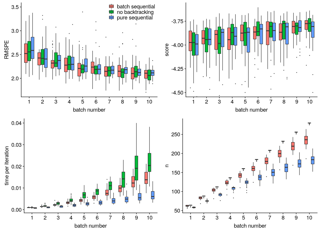
In terms of out-of-sample RMSPE and score, all methods exhibit similar performance. The purely sequential design method consistently yields more replicates. Thus, it also takes the lowest time per iteration for updating via hetGP. Our backtracking scheme yields a moderate proportion of replicates with the same performance as measured by RMSPE and score, compared to the version without backtracking. Notice that these metreics do not necessarily improve monotonically over batches. This could be attributed to unknown “true” mean and noise functions in this real-world simulator setting. Calculation of RMSPE and score are out-of-sample, on novel random testing sets, interjecting an extra degree of stochasticity in these assessments.

Appendix C Sanity check on batch acquisition

We returned to the 6d (4d manifold) pilot study of Section 2.3, involving $N=480$ runs, and inspected the properties of two new $M=24$-sized batches. To understand how these 48 inputs, selected via IMSPE and backtracking based on HetGP, compare to the original $n=96$-sized space-filling design, we plotted empirical densities of pairwise Euclidean distances within and between the two sets. See the solid-color-lined densities in the left panel of Figure 13. Dashed analogues offer a benchmark via sequential maximin design in two similarly sized batches. These represent an alternative, space-filling default, ignoring HetGP model fit/IMSPE acquisition criteria.

Figure 13: Empirical density of pairwise distances from IMSPE batch and maximin sequential design for the pilot (left) and full (right) studies.

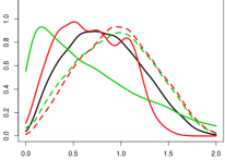
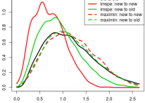
Consider first comparing the solid and dashed green lines, capturing the spread of distances between new and old runs. Observe that the solid-green density is shifted to the left relative to the dashed ones. This view reveals that IMSPE-selected runs are closer to the existing ones than they would be under a space-filing design. The solid-green density is similarly shifted left compared to distances from the old space-filling design (solid-black). The situation is a little different for distances within the new batches shown in red. Here we have a tighter density for IMSPE compared to space-filling, meaning we have fewer short and long distances – more medium ones. We take this as evidence that the HetGP/IMSPE batch scheme is working: spreading points out to a degree, but also focusing on some regions of the input space more than others.

The right panel of Figure 13 shows an analog of the comparison of pairwise distances for the larger smelt simulation campaign described in Section 6. In those 1056 new acquisitions, 204 involved replicates. With many more distance pairs, these kernel densities are more stable than in the 4d case on the left. Nonetheless, we observe a similar pattern here in 7d. IMSPE selections tend to be closer to themselves and to existing locations than ordinary space-filling ones would. We take this as an indication that the scheme was acting in a non-trivial way to reduce predictive uncertainty captured by HetGP model fits.

Appendix D Sensitivity indices for $m_{r}$

As we introduced in Section 2.1, $m_{r}$ is a parameter that describes the influence of water diversion facilities on $\lambda$. Here, we fix the two most influential factors, $m_{j}$ and $P_{j,3}$, at their respective default values of 0.015 and 0.6, to investigate sensitivity indices (based on our full analysis from Section 6) for other input factors.

Figure 14: Sensitivity analysis for mean (top) and variance process (bottom) with $m_{j}$ and $P_{j,3}$ fixed: main effects (left); first order (middle) and total sensitivity (right) from 100 bootstrap re-samples.

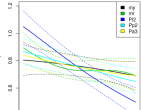
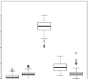
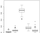
Observe in the top left panel of Figure 14 that, besides $m_{j}$ and $P_{j,3}$, $P_{l,2}$ also results in a relatively high variability of the mean response. Since the green curves are nonlinear, our analysis shows that $m_{r}$ plays a complicated role in the simulated population dynamics. Bottom panels of the figure show that $m_{r}$ settings drive variation in noise more than the remaining five input factors.

References

- Ankenman et al., (2010) Ankenman, B., Nelson, B. L., and Staum, J. (2010). “Stochastic kriging for simulation metamodeling.” Operations research, 58, 2, 371–382.
- Baker et al., (2020) Baker, E., Barbillon, P., Fadikar, A., Gramacy, R. B., Herbei, R., Higdon, D., Huang, J., Johnson, L. R., Ma, P., Mondal, A., Pires, B., Sacks, J., and Sokolov, V. (2020). “Stochastic Simulators: An Overview with Opportunities.”
- Barbieri et al., (2004) Barbieri, M. M., Berger, J. O., et al. (2004). “Optimal predictive model selection.” The annals of statistics, 32, 3, 870–897.
- Barnett, (1979) Barnett, S. (1979). Matrix Methods for Engineers and Scientists. McGraw-Hill.
- Baxter et al., (2015) Baxter, R., Brown, L. R., Castillo, G., Conrad, L., Culberson, S. D., Dekar, M. P., Dekar, M., Feyrer, F., Hunt, T., Jones, K., et al. (2015). “An updated conceptual model of Delta Smelt biology: our evolving understanding of an estuarine fish.” Tech. rep., Interagency Ecological Program, California Department of Water Resources.
- Bengtsson, (2018) Bengtsson, H. (2018). R.matlab: Read and Write MAT Files and Call MATLAB from Within R. R package version 3.6.2.
- Binois et al., (2018a) Binois, M., Gramacy, R. B., and Ludkovski, M. (2018a). “Practical Heteroscedastic Gaussian Process Modeling for Large Simulation Experiments.” Journal of Computational and Graphical Statistics, 27, 4, 808–821.
- Binois et al., (2018b) — (2018b). “Practical heteroskedastic Gaussian process modeling for large simulation experiments.” Journal of Computational and Graphical Statistics, 0, ja, 1–41.
- Binois et al., (2019) Binois, M., Huang, J., Gramacy, R. B., and Ludkovski, M. (2019). “Replication or Exploration? Sequential Design for Stochastic Simulation Experiments.” Technometrics, 61, 1, 7–23.
- Bisset et al., (2009) Bisset, K. R., Chen, J., Feng, X., Kumar, V. A., and Marathe, M. V. (2009). “EpiFast: a fast algorithm for large scale realistic epidemic simulations on distributed memory systems.” In Proceedings of the 23rd international conference on Supercomputing, 430–439.
- Byrd et al., (2003) Byrd, R., Lu, P., Nocedal, J., and Zhu, C. (2003). “A Limited Memory Algorithm for Bound Constrained Optimization.” SIAM Journal on Scientific Computing, 16.
- Carnell, (2020) Carnell, R. (2020). lhs: Latin Hypercube Samples. R package version 1.0.2.
- Chen et al., (2019) Chen, J., Mak, S., Joseph, V. R., and Zhang, C. (2019). “Adaptive design for Gaussian process regression under censoring.” arXiv preprint arXiv:1910.05452.
- Chevalier, (2013) Chevalier, C. (2013). “Fast uncertainty reduction strategies relying on Gaussian process models.” Ph.D. thesis, University of Bern.
- Cole et al., (2020) Cole, D. A., Christianson, R., and Gramacy, R. B. (2020). “Locally induced Gaussian processes for large-scale simulation experiments.” arXiv preprint arXiv:2008.12857.
- Duan et al., (2017) Duan, W., Ankenman, B. E., Sanchez, S. M., and Sanchez, P. J. (2017). “Sliced Full Factorial-Based Latin Hypercube Designs as a Framework for a Batch Sequential Design Algorithm.” Technometrics, 59, 1, 11–22.
- Erickson et al., (2018) Erickson, C. B., Ankenman, B. E., Plumlee, M., and Sanchez, S. M. (2018). “Gradient based criteria for sequential design.” In 2018 Winter Simulation Conference (WSC), 467–478.
- Fadikar et al., (2018) Fadikar, A., Higdon, D., Chen, J., Lewis, B., Venkatramanan, S., and Marathe, M. (2018). “Calibrating a stochastic, agent-based model using quantile-based emulation.” SIAM/ASA Journal on Uncertainty Quantification, 6, 4, 1685–1706.
- Farah et al., (2014) Farah, M., Birrell, P., Conti, S., and Angelis, D. D. (2014). “Bayesian emulation and calibration of a dynamic epidemic model for A/H1N1 influenza.” Journal of the American Statistical Association, 109, 508, 1398–1411.
- Ginsbourger and Le Riche, (2010) Ginsbourger, D. and Le Riche, R. (2010). “Towards Gaussian process-based optimization with finite time horizon.” In mODa 9–Advances in Model-Oriented Design and Analysis, 89–96. Springer.
- Ginsbourger et al., (2010) Ginsbourger, D., Le Riche, R., and Carraro, L. (2010). “Kriging is well-suited to parallelize optimization.” In Computational intelligence in expensive optimization problems, 131–162. Springer.
- Gneiting and Raftery, (2007) Gneiting, T. and Raftery, A. E. (2007). “Strictly Proper Scoring Rules, Prediction, and Estimation.” Journal of the American Statistical Association, 102, 477, 359–378.
- Gramacy and Polson, (2011) Gramacy, R. and Polson, N. (2011). “Particle learning of Gaussian process models for sequential design and optimization.” Journal of Computational and Graphical Statistics, 20, 1, 102–118.
- Gramacy, (2007) Gramacy, R. B. (2007). “tgp: An R Package for Bayesian Nonstationary, Semiparametric Nonlinear Regression and Design by Treed Gaussian Process Models.” Journal of Statistical Software, 19, 9, 1–46.
- Gramacy, (2020) — (2020). Surrogates: Gaussian Process Modeling, Design and Optimization for the Applied Sciences. Boca Raton, Florida: Chapman Hall/CRC. http://bobby.gramacy.com/surrogates/.
- Gramacy and Lee, (2009) Gramacy, R. B. and Lee, H. K. H. (2009). “Adaptive Design and Analysis of Supercomputer Experiment.” Technometrics, 51, 2, 130–145.
- Gramacy and Taddy, (2010) Gramacy, R. B. and Taddy, M. (2010). “Categorical Inputs, Sensitivity Analysis, Optimization and Importance Tempering with tgp Version 2, an R Package for Treed Gaussian Process Models.” Journal of Statistical Software, 33, 6, 1–48.
- Hamilton and Murphy, (2018) Hamilton, S. and Murphy, D. (2018). “Analysis of Limiting Factors Across the Life Cycle of Delta Smelt (Hypomesus transpacificus).” Environmental Management, 62.
- Herbei and Berliner, (2014) Herbei, R. and Berliner, L. M. (2014). “Estimating ocean circulation: an MCMC approach with approximated likelihoods via the Bernoulli factory.” Journal of the American Statistical Association, 109, 507, 944–954.
- Hong and Nelson, (2006) Hong, L. and Nelson, B. (2006). “Discrete Optimization via Simulation Using COMPASS.” Operations Research, 54, 1, 115–129.
- Johnson, (2008) Johnson, L. (2008). “Microcolony and Biofilm Formation as a Survival Strategy for Bacteria.” Journal of theoretical biology, 251, 24–34.
- Johnson et al., (1990) Johnson, M., Moore, L., and Ylvisaker, D. (1990). “Minimax and Maximin Distance Designs.” Journal of Statistical Planning and Inference, 26, 131–148.
- Jones et al., (1998) Jones, D., Schonlau, M., and Welch, W. J. (1998). “Efficient Global Optimization of Expensive Black Box Functions.” Journal of Global Optimization, 13, 455–492.
- Kennedy and Eberhart, (1995) Kennedy, J. and Eberhart, R. (1995). “Particle swarm optimization.” In Proceedings of ICNN’95 - International Conference on Neural Networks, vol. 4, 1942–1948 vol.4.
- Kennedy and O’Hagan, (2001) Kennedy, M. C. and O’Hagan, A. (2001). “Bayesian Calibration of Computer Models.” Journal of the Royal Statistical Society, Series B, 63, 425–464.
- Kimmerer and Rose, (2018) Kimmerer, W. and Rose, K. (2018). “Individual-Based Modeling of Delta Smelt Population Dynamics in the Upper San Francisco Estuary III. Effects of Entrainment Mortality and Changes in Prey.” Transactions of the American Fisheries Society, 147, 223–243.
- Leatherman et al., (2017) Leatherman, E. R., Santner, T. J., and Dean, A. M. (2017). “Computer experiment designs for accurate prediction.” Statistics and Computing, 1–13.
- Li and Deng, (2018) Li, Y. and Deng, X. (2018). “EI-Optimal Design: An Efficient Algorithm for Elastic I-optimal Design of Generalized Linear Models.” arXiv preprint arXiv:1801.05861.
- Loeppky et al., (2010) Loeppky, J. L., Moore, L. M., and Williams, B. J. (2010). “Batch sequential designs for computer experiments.” Journal of Statistical Planning and Inference, 140, 6, 1452–1464.
- Lund et al., (2010) Lund, J., Hanak, E., Fleenor, W., Bennett, W., and Howitt, R. (2010). Comparing Futures for the Sacramento, San Joaquin Delta, vol. 3. Univ of California Press.
- Lyu et al., (2018) Lyu, X., Binois, M., and Ludkovski, M. (2018). “Evaluating Gaussian process metamodels and sequential designs for noisy level set estimation.” arXiv preprint arXiv:1807.06712.
- MacNally et al., (2010) MacNally, R., Thomson, J., Kimmerer, W., Feyrer, F., Newman, K., Sih, A., Bennett, W., Brown, L., Fleishman, E., Culberson, S., and Castillo, G. (2010). “Analysis of pelagic species decline in the upper San Francisco Estuary using multivariate autoregressive modeling (MAR).” Ecological applications : a publication of the Ecological Society of America, 20, 1417–30.
- Marrel et al., (2009) Marrel, A., Iooss, B., Laurent, B., and Roustant, O. (2009). “Calculations of Sobol indices for the Gaussian process metamodel.” Reliability Engineering & System Safety, 94, 3, 742–751.
- Maunder and Deriso, (2011) Maunder, M. and Deriso, R. (2011). “A state-space multistage life cycle model to evaluate population impacts in the presence of density dependence: Illustrated with application to delta smelt (hyposmesus transpacificus).” Canadian Journal of Fisheries and Aquatic Sciences, 68, 1285–1306.
- Mckay et al., (1979) Mckay, D., Beckman, R., and Conover, W. (1979). “A Comparison of Three Methods for Selecting Vales of Input Variables in the Analysis of Output From a Computer Code.” Technometrics, 21, 239–245.
- McKeague et al., (2005) McKeague, I. W., Nicholls, G., Speer, K., and Herbei, R. (2005). “Statistical inversion of South Atlantic circulation in an abyssal neutral density layer.” Journal of Marine Research, 63, 4, 683–704.
- Mebane and Sekhon, (2011) Mebane, W. and Sekhon, J. (2011). “Genetic Optimization Using Derivatives: The rgenoud Package for R.” Journal of Statistical Software, 42, 1–26.
- Miller et al., (2012) Miller, W. J., Manly, B. F., Murphy, D. D., Fullerton, D., and Ramey, R. R. (2012). “An investigation of factors affecting the decline of delta smelt (Hypomesus transpacificus) in the Sacramento-San Joaquin Estuary.” Reviews in Fisheries Science, 20, 1, 1–19.
- Morris and Mitchell, (1995) Morris, M. D. and Mitchell, T. J. (1995). “Exploratory Designs for Computational Experiments.” Journal of Statistical Planning and Inference, 43, 381–402.
- Moyle et al., (2016) Moyle, P. B., Brown, L. R., Durand, J. R., and Hobbs, J. A. (2016). “Delta smelt: life history and decline of a once-abundant species in the San Francisco Estuary.” San Francisco Estuary and Watershed Science, 14, 2.
- Oakley and O’Hagan, (2004) Oakley, J. and O’Hagan, A. (2004). “Probabilistic sensitivity analysis of complex models: a Bayesian approach.” Journal of the Royal Statistical Society: Series B (Statistical Methodology), 66, 3, 751–769.
- Rose et al., (2013a) Rose, K. A., Kimmerer, W. J., Edwards, K. P., and Bennett, W. A. (2013a). “Individual-Based Modeling of Delta Smelt Population Dynamics in the Upper San Francisco Estuary: I. Model Description and Baseline Results.” Transactions of the American Fisheries Society, 142, 5, 1238–1259.
- Rose et al., (2013b) — (2013b). “Individual-Based Modeling of Delta Smelt Population Dynamics in the Upper San Francisco Estuary: II. Alternative Baselines and Good versus Bad Years.” Transactions of the American Fisheries Society, 142, 5, 1260–1272.
- Rutter et al., (2019) Rutter, C. M., Ozik, J., DeYoreo, M., Collier, N., et al. (2019). “Microsimulation model calibration using incremental mixture approximate Bayesian computation.” The Annals of Applied Statistics, 13, 4, 2189–2212.
- Sacks et al., (1989) Sacks, J., Welch, W., J. Mitchell, T., and Wynn, H. (1989). “Design and analysis of computer experiments. With comments and a rejoinder by the authors.” Statistical Science, 4.
- Saltelli et al., (2000) Saltelli, A., Chan, K., and Scott, M. (2000). Sensitivity Analysis. New York, NY: John Wiley & Sons.
- Santner et al., (2018) Santner, T., Williams, B., and Notz, W. (2018). The Design and Analysis of Computer Experiments, Second Edition. New York, NY: Springer–Verlag.
- Seo et al., (2000) Seo, S., Wallat, M., Graepel, T., and Obermayer, K. (2000). “Gaussian Process Regression: Active Data Selection and Test Point Rejection.” In Proceedings of the International Joint Conference on Neural Networks, vol. III, 241–246. IEEE.
- Stein, (2012) Stein, M. (2012). Interpolation of Spatial Data: Some Theory for Kriging. New York, NY: Springer Science & Business Media.
- Stompe et al., (2020) Stompe, D. K., Moyle, P. B., Kruger, A., and Durand, J. R. (2020). “Comparing and Integrating Fish Surveys in the San Francisco Estuary: Why Diverse Long-Term Monitoring Programs are Important.” San Francisco Estuary and Watershed Science, 18, 2.
- Taddy et al., (2009) Taddy, M., Lee, H., Gray, G., and Griffin, J. (2009). “Bayesian guided pattern search for robust local optimization.” Technometrics, 51, 4, 389–401.
- Thomson et al., (2010) Thomson, J., Kimmerer, W., Brown, L., Newman, K., Mac Nally, R., Bennett, W., Feyrer, F., and Fleishman, E. (2010). “Bayesian change point analysis of abundance trends for pelagic fishes in the upper San Francisco Estuary.” Ecological applications : a publication of the Ecological Society of America, 20, 1431–48.
- Wycoff et al., (2019) Wycoff, N., Binois, M., and Wild, S. M. (2019). “Sequential Learning of Active Subspaces.”
- Xie et al., (2012) Xie, J., Frazier, P. I., Sankaran, S., Marsden, A., and Elmohamed, S. (2012). “Optimization of computationally expensive simulations with Gaussian processes and parameter uncertainty: Application to cardiovascular surgery.” In 2012 50th Annual Allerton Conference on Communication, Control, and Computing (Allerton), 406–413.
- Yu, (2002) Yu, H. (2002). “Rmpi: Parallel Statistical Computing in R.” R News, 2, 2, 10–14.