Quantum dynamics and relaxation
in comb turbulent diffusion
[ Chaos, Solitons & Fractals 139 (2020) 110305 ]

Abstract

Continuous time quantum walks in the form of quantum counterparts of turbulent diffusion in comb geometry are considered. The interplay between the backbone inhomogeneous advection $\delta(y)x\partial_{x}$ along the $x$ axis, which takes place only at the $y=0$, and normal diffusion inside fingers $\partial_{y}^{2}$ along the $y$ axis leads to turbulent diffusion. This geometrical constraint of transport coefficients due to comb geometry and properties of a dilatation operator lead to consideration of two possible scenarios of quantum mechanics. These two variants of continuous time quantum walks are described by non-Hermitian operators of the form $\hat{{\cal H}}=\hat{A}+i\hat{B}$. Operator $\hat{A}$ is responsible for the unitary transformation, while operator $i\hat{B}$ is responsible for quantum/classical relaxation. At the first quantum scenario, the initial wave packet can move against the classical streaming. This quantum swimming upstream is due to the dilatation operator, which is responsible for the quantum (not unitary) dynamics along the backbone, while the classical relaxation takes place in fingers. In the second scenario, the dilatation operator is responsible for the quantum relaxation in the form of an imaginary optical potential, while the quantum unitary dynamics takes place in fingers. Rigorous analytical analysis is performed for both wave and Green’s functions.

1 Introduction

We consider a quantum dynamics, which is a quantum counterpart of turbulent diffusion in comb geometry. A possible realization of the turbulent transport can be discussed in the framework of a Langevin equation in a so-called Matheron - de Marsily form [1],

$$\dot{x_{1}}=\delta(x_{2})vx_{1}\,\quad\dot{x_{2}}=\eta(t)\,.$$ (1.1)

Here $\eta(t)$ is a random Gaussian delta correlated process $\langle\eta(t)\eta(t^{\prime})\rangle=2D\delta(t-t^{\prime})$, where $D$ is a diffusion coefficient. In this case, white noise in the $x_{2}$ axis affects the velocity of inhomogeneous advection along the $x_{1}$ axis at $x_{2}=0$. Introducing a probability distribution function (PDF) $P(x,y,t)=\langle\delta(x_{1}-x)\delta(x_{2}-y)\rangle$, we obtain a Fokker-Planck equation (FPE) in the form of a 2D comb model [2]

$$\partial_{t}P(x,y,t)=-v\delta(y)\partial_{x}xP(x,y,t)+D\partial_{y}^{2}P(x,y,t)\,.$$ (1.2)

The comb Eq. (1.2) has been considered in Ref. [2] as a realistic mechanism of superdiffusion of heavy particles, related to various applications. Important role in this turbulent acceleration of the comb transport and superdiffusion plays inhomogeneous advection in the form of a dilatation operator. In the Hamiltonian form, the dilatation (contraction) operator

$$\hat{{\cal H}}_{0}=-ix\hbar\frac{d}{dx}-i\hbar/2\equiv x\hat{p}_{x}-i\hbar/2$$ (1.3)

attracts much attention in quantum mechanics and number theory in connection with the Riemann zeros. This operator has been suggested by Berry and Keating [3, 4, 5] in connection to the Riemann Hypothesis, and $\hat{\cal H}_{0}$ is known as a Berry-Keating-Connes Hamiltonian [6]. In a more general content, the operator has been considered as a generator of space-time conformal transformations [7, 8] and entropy problem in quantum mechanics [9], a random walk approximation to the Riemann Hypothesis [10], and the quantum Mellin transform [11]. Also it corresponds to quantum dynamics in inverted potentials [12], and near hyperbolic points [13], including singular behavior [14] and exponential spreading of the phase space [15]. In comb geometry, this operator leads to the exponential spread of the phase space as well [16]. Recently, it has been considered as a turbulent diffusion search optimisation [17].

Due to the comb geometry, the backbone inhomogeneous advection along the $x$ axis acts only at the $y=0$. This geometrical constraint of transport coefficients leads (at least) to two possible scenarios of quantum mechanical transport related to turbulent diffusion described by Eq. (1.2). In particular, the comb FPE (1.2) has straightforward relation to quantum mechanics. It is just a one dimensional quantum mechanical problem at $y=0$ with the backbone Schrödinger equation $i\hbar\partial_{t}\psi(x,t)=-iv\hbar x\partial_{x}\psi(x,t)$. The classical PDF is mapped on the wave/Green’s functions: $P(x,y=0,t)\rightarrow\psi(x,t)/G_{x}(x,t)$. In this case, one can consider the quantum dynamics governed by the non-Hermitian Hamiltonian according to the Schrödinger equation

$$i\hbar\partial_{t}\psi(x,y,t)=\hat{{\cal H}}\psi(x,y,t)=\left[v\delta(y)\hat{\cal H}_{0}-\tfrac{iD}{\hbar}\hat{p}_{y}^{2}\right]\psi(x,y,t)\,.$$ (1.4)

In this case, the quantum (non-unitary) dynamics inside the backbone along the $x$ axis at $y=0$ is accompanied by relaxation due to diffusion inside fingers along the $y$ axis.

The second scenario is according to the Wick rotation of time $t\rightarrow it$ with $D=\hbar/2m$, where $m=1$ is a unit mass of a quantum particle. Then the non-Hermitian Hamiltonian is

$$\hat{\cal H}=\hat{p}_{y}^{2}/2+i\hat{\cal H}_{0}\delta(y)\equiv\hat{A}+i\hat{B}\,.$$ (1.5)

In this case, the backbone is a quantum trap for the $y$ axis transport, where relaxation is due to the dilatation operator $\hat{\cal H}_{0}$, which works now as a scattering. This approach is a generalization of the dynamics of quantum particles in the presence of traps due to a complex optical potential [19, 20].

2 Turbulent diffusion

In this section, we consider the comb Eq. (1.2) as a realistic mechanism of exponential (or turbulent) superdiffusion and extend a picture of possible solutions of the problem, described in Ref. [2]. For the completeness of the presentation we first consider the logarithmic scale of possible solutions.

2.1 Logarithmic scale

Let us consider dynamics for $x(x_{1})>0$. Following to Ref. [11], we introduce new variable $w=\ln(x_{1})$, and Eq. (1.1) reads

$$\dot{w}=v\delta(x_{2}),\quad\dot{x_{2}}=\eta(t)\,.$$ (2.1)

The comb Fokker-Planck equation (1.2) in the log scale for the PDF $P=P(w,y,t)$ now reads

$$\partial_{t}P=-v\delta(y)\partial_{w}P+D\partial_{y}^{2}P$$ (2.2)

with the initial condition $P_{0}(w,y)=\frac{1}{x}\delta(w-w_{0})\delta(y)=e^{-w}\delta(w-w_{0})\delta(y)$ and $w\in(-\infty\,,\infty)$. After the Laplace transform with respect to $t$, we look for the solution in the form

$$P(w,y,s)={\cal L}\left[P(w,y,t)\right](s)=f(w,s)g(y,s)=f(w,s)\exp\left(-|y|\sqrt{s/D}\right)\,.$$ (2.3)

This yields

$$v\partial_{w}f(w,s)+2\sqrt{Ds}f(w,s)=\frac{1}{x}\delta(w-w_{0})\,.$$ (2.4)

We obtain the PDF of the backbone diffusion as follows

$$f(w,t)\equiv P(w,y=0,t)=\\ =\frac{(w-w_{0})D}{\sqrt{\pi t^{3}v^{2}}}\exp\left(-\frac{D(w-w_{0})^{2}}{tv^{2}}\right)e^{-w}\theta(w-w_{0})\,.$$ (2.5)

In the $x$ space, it corresponds to the log-normal distribution

$$P(x,y=0,t)=\frac{D\ln(x/x_{0})}{x\sqrt{\pi t^{3}v^{2}}}\times\exp\left(-\frac{D\ln^{2}(x/x_{0})}{tv^{2}}\right)\theta(x-x_{0})\,.$$ (2.6)

Solution in Eq. (2.6) can be extended on $x<0$. Introducing symmetric initial condition $\frac{1}{2}[\delta(x-a)+\delta(x+a)]$ at the backbone, one obtains

$$P(x,y=0,t)=\frac{\ln(|x|/a)}{2|x|\sqrt{\pi t^{3}v^{2}/D}}\times\exp\left(-\frac{\ln^{2}(|x|/a)}{tv^{2}/D}\right)\theta(|x|-a)\,.$$ (2.7)

2.2 Symmetric solution

Let us consider the comb equation (1.2) with a symmetrical initial condition at $(x,y)=(\pm a,0)$: $P_{0}(x,y)=\delta(y)[\delta(x-a)+\delta(x+a)]/2$, where $a>0$. Taking into account the Laplace transformation with respect to $t$ and ansatz $P(x,y,s)=f(x,s)\exp\left(-|y|\sqrt{s/D}\right)$, we obtain

$$vx\partial_{x}f+(2\sqrt{Ds}+v)f=\delta(|x|-a)/2\,,$$ (2.8)

where $x\in(-\infty\,,\infty)$ and $\delta(|x|-a)\equiv\delta(x-a)+\delta(x+a)$. The solution of Eq. (2.8) is $f(x,s)=C|x/a|^{-\mu(s)}\theta(|x|-a)$, where $\mu(s)=2\sqrt{Ds}/v+1$. We also take into account that $\partial_{x}|x|=\rm{sgn}(x)=2\theta(x)-1$, and $\rm{sgn(x)}|x|=x$. An arbitrary constant $C$ is determined from the normalization condition of $P(x,y,s)$. Therefore, we obtain a “dead zone” in $x\in(-a,a)$ with $f(x,t)=0$ and log normal distribution according Eq. (2.7) for $|x|\geq a$. The “dead zone” is due to the initial condition at $x=\pm a\neq 0$ and directional outward streaming from $x=\pm a$ to $x\rightarrow\pm\infty$. For $a=0$, the solution of Eq. (2.8) reads [2] $f(x,s)=C|x|^{1-\mu(s)}+\delta(x)/(\mu(s)-1)$. In this case, the PDF consists of two parts: the log-normal distribution, which contributes to the exponentially fast spreading and the second part is due to the pining delta function. The latter does not contribute to the mean squared displacement (MSD).

Correspondingly, the solution for the PDF $P(x,y,t)$ is a convolution integral

$$P(x,y,t)=P(x,y=0,t)\ast P_{y}(y,t)=\int_{0}^{t}P(x,y=0,t-t^{\prime})P_{y}(y,t^{\prime})dt^{\prime}\,,$$ (2.9)

where $P(x,y=0,t)=f(x,t)$ and $P_{y}(y,t)$ is the Lévy-Smirnov density defined by the inverse Laplace transform,

$$P_{y}(y,t)={\cal L}^{-1}\left\{\exp[-|y|\sqrt{s/D}]\right\}\,.$$ (2.10)

3 Quantum dynamics: Eigenvalue’s expansion

We consider two scenarios of the quantum dynamics described by non-Hermitian operators. The first one is the quantum dynamics along the backbone with relaxation in the form of classical diffusion along the fingers. Contrary to that, the second scenario is the quantum dynamics in fingers while relaxation in the backbone is due to the dilatation operator. In both cases, the dilatation operator $H_{0}$ plays important role for the quantum tasks. Therefore we start from the eigenvalue problem of the dilatation operator.

The dilatation operator (1.3)

$$\hat{{\cal H}}_{0}=\hbar[-ix\partial_{x}-i/2]=\hat{p}_{x}x+i\hbar/2$$

determines the complete set of eigenfunctions $\chi_{\omega}(x)$ with the eigenvalues $\omega$ according to the eigenvalue problem $\hat{{\cal H}}\chi_{\omega}(x)=\hbar\omega\chi_{\omega}(x)$, where $\omega$ is the continuous spectrum and the eigenfunctions are [3, 6]

$$\chi_{\omega}(x)=\frac{1}{\sqrt{N|x|}}\exp[i\omega\ln|x|]\,,$$ (3.1)

which satisfies the boundary conditions $\chi_{\omega}(x=\pm\infty)=0$ and $N=4\pi$. For the continuous spectrum, the normalization condition is

$$\int_{-\infty}^{\infty}\chi_{\omega^{\prime}}^{*}(x)\chi_{\omega}(x)dx=\delta(\omega-\omega^{\prime})\,,$$ (3.2)

while the completeness relation is $\int\chi_{\omega}^{*}(x^{\prime})\chi_{\omega}(x)d\omega=\delta(x-x^{\prime})$ (see e.g. [22]). Note also that for $x>0$ the normalization constant is half as larger, $N=2\pi$ [6].

It is worth mentioning that a mathematically rigorous calculation of the normalization constant for the wave function $\chi_{\omega}(x)$ can be presented by following the presentation due to the monograph by V.A. Fock [21]. Since the operator $x\hat{p}$ has continuous spectrum $\omega$, the eigenfunctions $\chi(\omega,x)\equiv\chi_{\omega}(x)$ are not square integrable. Therefore, the normalization condition exists not for the eigenfunction but for the “eigendifferential” [21] $\Delta\chi(\omega,x)$, which reads $\Delta\chi(\omega,x)=\int_{\omega}^{\omega+\Delta\omega}\chi(\omega^{\prime},x)d\omega^{\prime}$. Substituting here Eq. (3.1), one obtains

$$\Delta\chi(\omega,x)=\frac{2}{\sqrt{N|x|}\ln|x|}\exp[i(\omega+\Delta\omega)\ln|x|]\sin\frac{\Delta\omega\ln|x|}{2}\,.$$

This solution is already square integrable and has the normalization form

$$\lim_{\Delta\omega\to 0}\frac{1}{\Delta\omega}\int_{-\infty}^{\infty}dx\left|\Delta\chi(\omega,x)\right|^{2}=1\,.$$ (3.3)

To take the limit in Eq. (3.3), the integrand can be presented as follows

$$\left|\Delta\chi(\omega,x)\right|^{2}=\frac{4}{N|x|\ln^{2}|x|}\sin\frac{\Delta\omega\ln|x|}{2}\sin\frac{\Delta\Omega\ln|x|}{2}\,,$$

where $\Delta\Omega=\Delta\omega+\Delta\omega_{1}$. We can perform this trick, since the “eigendifferentials” for not overlapping spectral regions $\Delta\omega$ and $\Delta\omega_{1}$ are orthogonal. [21]. Then taking the limit $\Delta\omega=0$ and carrying out the variable change $z=(\Delta\omega_{1}/2)\ln|x|$ and taking into account that $\frac{4}{N}\int_{-\infty}^{\infty}\frac{\sin z}{z}dz=\frac{4\pi}{N}$, we obtain $N=4\pi$, which coincides exactly with the dimensionless normalization constant $N$ in Eq. (3.1).

4 Quantum dynamics in backbone

The Schrödinger equation (1.4) for the Green’s function, described the dynamics of the first scenario, is

$$i\hbar\partial_{t}G(x,y,t)=v\delta(y)(x\hat{p}_{x}-i\hbar/2)G(x,y,t)-\tfrac{iD}{\hbar}\hat{p}_{y}^{2}G(x,y,t)$$ (4.1)

with the initial condition $G(x,y,t=0)=\delta(x-x_{0})\delta(y)$ and $D=\hbar/2$. In the Laplace domain ${\cal L}[\psi(t)](s)=\tilde{\psi}(s)$, Eq. (4.1) reads

$$is\hbar\tilde{G}(x,y,s)=v\delta(y)(x\hat{p}_{x}-i\hbar/2)\tilde{G}(x,y,s)\\ -\tfrac{iD}{\hbar}\hat{p}_{y}^{2}\tilde{G}(x,y,s)-i\hbar\delta(x-x_{0})\delta(y)\,.$$ (4.2)

The Laplace image of the Green’s function has the multiplicative form of both backbone and finger’s dynamics

$$\tilde{G}(x,y,s)=\tilde{G}(x,y=0,s)g(y,s)=f(x,s)e^{-|y|\sqrt{s/D}}\,,$$ (4.3)

where $g(y,s)=e^{-\sqrt{s/D}|y|}$ describes relaxation of quantum dynamics in the form of classical diffusion in fingers, while $f(x,s)$ describes the quantum dynamics in the backbone. Substituting solution (4.3) in Eq. (4.2), we obtain equation for the backbone quantum dynamics

$$-iv(x\partial_{x}+\tfrac{1}{2})f(x,s)-i\sqrt{2\hbar s}f+i\delta(x-x_{0})=0.$$ (4.4)

Formally, it corresponds to the PDF of classical diffusion, described in Sec. 2.2, with $\mu(s)=1+\sqrt{2\hbar s}/v$. When $x_{0}=0$, the solution reads

$$f(x,s)=|x|^{\tfrac{1}{2}-\mu(s)}+\delta(x)/[\mu(s)-1/2]\,.$$ (4.5)

Further quantum mechanical analysis is carried out in the framework of the spectral decomposition according to the eigenvalue problem of Sec. 3. Since $\chi_{\omega}(x)$ is a complete set of eigenfunction, $f(x,s)$ can be considered as a superposition

$$f(x,s)=\int d\omega\chi_{\omega}(x)b_{\omega}(s)\,.$$ (4.6)

From Eq. (4.4), this yields equation for $b_{\omega}(s)\equiv b(s)$ as follows

$$v\omega b(s)-i\sqrt{2\hbar s}b(s)=-i\chi^{*}_{\omega}(x_{0})\,.$$ (4.7)

Resolving this equation with respect to $b(s)$ and substituting it in Eq. (4.6), we obtain

$$f(x,s)=\frac{1}{iv}\int\frac{d\omega\chi_{\omega}(x)\chi^{*}_{\omega}(x_{0})}{\omega-i\sqrt{2\hbar s}/v}=\\ =\frac{1}{4\pi iv|x|}\int\frac{d\omega e^{i\omega\ln|x/x_{0}|}}{\omega-i\sqrt{2\hbar s}/v}=\\ =\frac{1}{2v|x|}e^{-\sqrt{2\hbar s}\ln|x/x_{0}|/v}\,,$$ (4.8)

where $x>x_{0}$ for $\rm{Re}\sqrt{s}>0$ and $x<x_{0}$ if $\rm{Re}\sqrt{s}<0$. We note that there is no anymore the “dead zone”, and this quantum situation changes drastically from classical turbulent diffusion discussed in Sec. 2. We call this effect a quantum swimming upstream.

Substituting the result of Eq. (4.8) in Eq. (4.3), we obtain the Green’s function in the form of the Laplace inversion

$$G(x,y,t)=\frac{1}{2v|x|}{\cal L}^{-1}\left[e^{-(v|y|+\ln|x/x_{0}|)\sqrt{2s\hbar}/v}\right]=\\ =\frac{(v|y|+\ln|x/x_{0}|)}{4v^{2}|x|\sqrt{2\pi t^{3}/\hbar}}\exp\left[-\hbar\frac{(v|y|+\ln|x/x_{0}|)^{2}}{2v^{2}t}\right]\,,$$ (4.9)

which is the quantum Green’s function in the form of the combination of the log-normal and Lévy-Smirnov densities.

4.1 Fractional dynamics in backbone

Let us show that behind this classical Lévy-Smirnov form of the Green’s function there is a fractional quantum dynamics along the backbone. To this end, let us perform the Laplace inversion before performing integration with respect to the spectrum in Eq. (4.8). Then the expansion coefficient $b_{\omega}(s)$ in Eq. (4.7) reads

$$b_{\omega}(s)=\frac{A_{\omega}(x_{0})}{\sqrt{s}+i\tilde{\omega}}\,,$$ (4.10)

where $\tilde{\omega}=v\omega/\sqrt{2\hbar}$ and $A_{\omega}(x_{0})=\chi^{*}_{\omega}(x_{0})/\sqrt{2\hbar}$. Performing the Laplace inversion, we obtain the temporal behavior of the coefficients in the form of the Mittag-Leffler functions $E_{\alpha,\beta}(z)$ [23]:

$$B_{\omega}(t)={\cal L}^{-1}[b_{\omega}(s)](t)=A_{\omega}(x_{0})t^{-\frac{1}{2}}E_{\frac{1}{2},\frac{1}{2}}\left(-i\tilde{\omega}t^{\frac{1}{2}}\right)\,.$$ (4.11)

Therefore, the backbone component of the Green’s function reads

$$f(x,t)=\int B_{\omega}(t)\chi_{\omega}(x)d\omega=\\ =\frac{1}{\sqrt{2\hbar t}}\int d\omega\chi^{*}_{\omega}(x_{0})E_{\frac{1}{2},\frac{1}{2}}\left(-i\tilde{\omega}t^{\frac{1}{2}}\right)\chi_{\omega}(x)=\\ =\frac{1}{\sqrt{2\hbar t}}E_{\frac{1}{2},\frac{1}{2}}\left(-i\hat{H}t^{\frac{1}{2}}\right)\delta(x-x_{0})\equiv G_{x}\left(i\hat{{\cal H}}t^{\frac{1}{2}}\right)\,,$$ (4.12)

where the “Hamiltonian” is $\hat{{\cal H}}=\tfrac{v\hat{\cal H}_{0}}{\sqrt{2\hbar}}$.

The Green’s function is the convolution of two non-unitary dynamics, which are the quantum fractional dynamics along the backbone with the Green’s function $G_{x}(x,t)=f(x,t)$ and the finger’s dynamics according to the Lévy-Smirnov density

$$G_{y}(y,t)={\cal L}^{-1}\left[\exp\left(-|y|\sqrt{2s\hbar}\right)\right](t)=\frac{\hbar|y|}{\sqrt{\pi t^{3}}}\exp\left(-\hbar\frac{y^{2}}{2t}\right)\,.$$ (4.13)

That is

$$G(x,y,t)=G_{x}\left(\hat{{\cal H}}t^{\frac{1}{2}}\right)\ast G_{y}(y,t),$$ (4.14)

which yields the result in Eq. (4.9). Therefore, the quantum dynamics at the backbone is not unitary.

5 Fox H function for quantum swimming upstream

The Mittag-Leffler function can be presented in the form of the Fox $H$ function [24] (see also Exampl. 2.7 in Ref. [25]) defined in terms of the Mellin-Barnes integral,

$$E_{\alpha,\beta}(-z)=H^{1,1}_{2,1}(z)=\frac{1}{2\pi i}\int_{C}\frac{\Gamma(\xi)\Gamma(1-\xi)}{\Gamma(\beta-\alpha\xi)}(z)^{-\xi}d\xi\,,$$ (5.1)

where $\Gamma(\xi)$ is a gamma function and the contour $C$ starts at $c-i\infty$, ends at $c+i\infty$ and separates the poles of the gamma functions $\Gamma(\xi)$ and $\Gamma(1-\xi)$, such that $0<\rm{Re}(\xi)<1$. In Eq. (5.1), $z=i\tilde{\omega}t^{\frac{1}{2}}$ is the imaginary variable and $\alpha=\beta=1/2$. Integration with respect to the spectrum reads

$$I(x/x_{0})=\frac{1}{4\pi|x|}\int_{-\infty}^{\infty}(i\omega)^{-\xi}e^{i\omega\ln|x/x_{0}|}d\omega\,.$$ (5.2)

To perform this integration, the variable change $i\omega=\tau$ yields the standard Laplace inversion

$$I(x/x_{0})=\frac{1}{2|x|}\cdot\frac{1}{2\pi i}\int_{-i\infty}^{i\infty}\tau^{-\xi}e^{w\tau}d\tau=\frac{w^{\xi-1}}{2|x|\Gamma(\xi)}\,,$$ (5.3)

where $w\equiv w(x/x_{0})=\ln|x/x_{0}|>0$ and $0<\rm{Re}(\xi)<1$. When $w<0$, it means that a quantum particle is in the dead zone $|x|<|x_{0}|$, then the variable change is $\tau=-i\omega$. The integral in Eq. (5.3) reads

$$I(x/x_{0})=\frac{1}{2|x|}\frac{1}{2\pi i}\int_{-i\infty}^{i\infty}(-\tau)^{-\xi}e^{\tau|w|}d\tau=\frac{e^{-i\pi\xi}|w|^{\xi-1}}{2|x|\Gamma(\xi)}=-\frac{w^{\xi-1}}{2|x|\Gamma(\xi)}\,.$$ (5.4)

Therefore, taking into account results in Eqs. (5.1) - (5.4) for the integration (4.12). we obtain the backbone Green’s function as follows

$$G_{x}(x,t)\equiv f(x,t)=\int B_{\omega}(t)\chi_{\omega}(x)d\omega=\\ =\pm\frac{w^{-1}}{2|x|\sqrt{2\hbar t}}\frac{1}{2\pi i}\int_{C}\frac{\Gamma(1-\xi)}{\Gamma(\frac{1}{2}-\frac{1}{2}\xi)}\left(\frac{vt^{\frac{1}{2}}}{w\sqrt{2\hbar}}\right)^{-\xi}d\xi\,,$$ (5.5)

where $(+)$ sign is for $w>0~{}(|x/x_{0}|>1)$ and $(-)$ sign is for $w<0~{}(|x/x_{0}|<1)$. Now, using the Legendre duplication formula, $\Gamma(z)\Gamma(z+1/2)=2^{1-2z}\sqrt{\pi}\Gamma(2z)$, which yields $\tfrac{\Gamma(1-\xi)}{\Gamma(1/2-\xi/2)}=2^{-\xi}\Gamma(1-\xi/2)/\sqrt{\pi}$. Defining $p=1-\xi/2$, we obtain Eq. (5.5) as follows (see e.g., Eq. (2.43) in Ref. [25])

$$G_{x}(x,t)=\pm\frac{w^{-1}}{2|x|\sqrt{2\pi\hbar t}}\\ \times\frac{\hbar w^{2}}{2v^{2}t}\frac{1}{2\pi i}\int_{C}\left(\frac{\hbar w^{2}}{2v^{2}t}\right)^{-p}\Gamma(p)dp=\\ =\pm\frac{\ln\left|\tfrac{x}{x_{0}}\right|}{4|x|v^{2}\sqrt{2\pi t^{3}/\hbar}}\exp\left[-\hbar\frac{\ln^{2}\left|\tfrac{x}{x_{0}}\right|}{2v^{2}t}\right]\,.$$ (5.6)

The Green’s function in Eq. (5.6) is a more accurate result on the quantum dynamics inside the “dead zone” for $|x|<|x_{0}|$. It contains the phase multiplier $e^{-i\pi}$, which corresponds to the quantum swimming upstream.

6 Quantum dynamics in fingers

In this section we consider the second scenario, which is performed according to the Wick rotation of time $t\rightarrow it$ in Eq. (1.2) with $D=\hbar/2m$, and $m=1$ is a unit mass of a quantum particle. Then the Schrödinger equation reads

$$i\hbar\partial_{t}\psi(x,y,t)=\hat{\cal H}\psi(x,y,t)\,,$$ (6.1)

where the non-Hermitian Hamiltonian is $\hat{\cal H}=\hat{p}_{y}^{2}/2+iv\hat{\cal H}_{0}\delta(y)$. An important point of the analysis should be admitted: it is the imaginary optical potential, which acts as a trap [19, 20, 26]. In the finger’s quantum dynamics the trap relates to the dilatation operator and leads to the imaginary delta function, see also A. To understand this phenomenon, the dynamics of both the wave and Green’s functions is analysed.

Again, we consider the wave function as a decomposition over the complete set $\chi_{\omega}(x)$,

$$\psi(x,y,t)=\int\phi_{\omega}(y,t)\chi_{\omega}(x)d\omega\,.$$ (6.2)

Then taking into account properties of the dilatation/contraction operator $\hat{\cal H}_{0}$ and owing to Eq. (6.2), we present the initial condition as the spectral decomposition as well with the Gaussian weight $\rho_{a}(\omega)=\left[\frac{2a}{\pi}\right]^{\frac{1}{4}}\exp(-a\omega^{2})$ with real $a>0$ [15]. This yields the initial condition for the backbone wave function in the form of a log-normal distribution. Eventually, we obtain the initial condition for $\phi_{\omega}(y,t=0)$ as follows

$$\phi_{\omega}(y,t=0)=\rho_{a}(\omega)\Phi_{0}(y,\omega)\,,$$ (6.3)

where the choice of $\Phi_{0}(y,\omega)$ depends on the choice of the boundary conditions for every $\omega$ mode. In particular, free boundary conditions is considered in what follows.

6.1 Wave function

In the case of free conditions at the boundaries of the fingers, we arrive at the $y$ transport in the form of a scattering problem with the imaginary potential $iv\hbar\omega\delta(y)$ as follows

$$i\hbar\partial_{t}\phi_{\omega}=-\frac{\hbar^{2}}{2}\partial_{y}^{2}\phi_{\omega}+iv\hbar\omega\delta(y)\phi_{\omega}\,.$$ (6.4)

Looking for the eigenvalue solutions $\phi_{\omega}(y,t)=e^{-iet/\hbar}\Phi_{e}(y)$, we arrive at the eigenvalue problem

$$-\frac{\hbar^{2}}{2}\partial_{y}^{2}\Phi_{e}+i\lambda\delta(y)\Phi_{e}=e\Phi_{e}\,,$$ (6.5)

with free boundary conditions at infinities and $\lambda=\hbar v\omega$. Contrary to the real (attractive) delta potential [27], there are no bound states. However, still we can consider two classes of the spectrum [25, 27]. The first class corresponds to the scattering problem and contains the continuous spectrum solutions, which are standing waves. The solutions can be considered as the result of the scattering by the $i\delta$ potential of the left and right incident waves [27],

$$\Phi^{\pm}_{k}(y)=\frac{1}{\sqrt{2\pi}}\left[e^{\pm iky}+\mathcal{B}(k)e^{ik\lvert y\rvert}\right],$$ (6.6)

where $\mathcal{B}(k)={\lambda}/{(\hbar^{2}k-\lambda)}$ is the “scattering amplitude”, determined by Eq. (6.5) and related to imaginary potential, and $e=e(k)=\hbar^{2}k^{2}/2$.

In further analysis we are interesting in the second class of the solutions, which is but one (not bound) state

$$\Phi_{0}(y)=(-i\lambda)^{1/2}e^{i\lambda|y|}\,,\quad e_{0}=\lambda^{2}/2\,.$$ (6.7)

We choose $\Phi_{0}(y,\omega)=\Phi_{0}(y)$ to be the initial condition for the finger’s quantum dynamics. This immediately yields the quantum evolution of the finger’s wave function

$$\phi_{\omega}(y,t)=(-i\hbar\omega v)^{\frac{1}{2}}e^{-i\frac{\hbar}{2}(\omega v)^{2}t}\cdot e^{i\hbar\omega v|y|}\,$$ (6.8)

and the dynamics (including the initial condition) of the comb wave function reads from Eqs. (6.2) and (6.3), and (6.8) as follows

$$\psi(x,y,t)=\frac{(-i\hbar v)^{\frac{1}{2}}}{\sqrt{4\pi|x|}}\left[\frac{2a}{\pi}\right]^{\frac{1}{4}}\times\int_{-\infty}^{\infty}\frac{e^{-A(t)\omega^{2}}}{\omega^{\frac{1}{2}}}e^{i\omega(\hbar v|y|+\ln|x|)}d\omega\,,$$ (6.9)

where $A(t)=a+i\hbar v^{2}t$. When $t=0$ it corresponds to the initial condition of the comb wave function. The exact solution of the wave function is expressed in the form of the hypergeometric and Bessel functions. However it is instructive to present the result in the form of elementary functions. To this end, the integral in Eq. (6.9) is evaluated by the stationary phase approximation, which yields

$$\psi(x,y,t)=\frac{i(\hbar v)^{\frac{1}{2}}}{\sqrt{|x|(\hbar v|y|+\ln|x|)}}\cdot\left[\frac{a}{2\pi}\right]^{\frac{1}{4}}\times\exp\left[-\frac{(\hbar v|y|+\ln|x|)^{2}}{(a+i\hbar v^{2}t)}\right]\,.$$ (6.10)

6.2 Green’s function

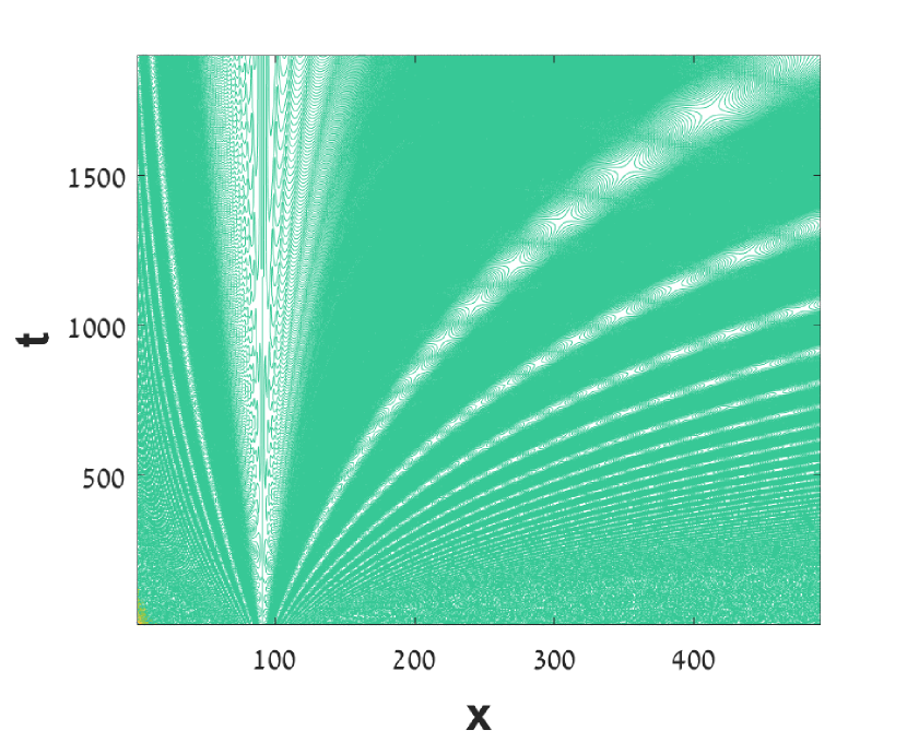
Figure 1: Contour presentation of the real part of Green’s function (6.13) as a function of $t$ and $x$ for $t\in[10^{-5}\,,2\cdot 10^{-4}]$ and $x\in[10^{-1}\cdot x_{0}\,,5\cdot x_{0}]$, where the initial condition $x_{0}=10^{-3}$. The imaginary part exhibits the same $x-t$ structure. All parameter and constants are taken in dimensionless form such that $\sqrt{\hbar}=2v$. The contour is plotted on $x-t$ grid with $\Delta x=10^{-5}$ and $\Delta t=10^{-7}$. In the case the axes are measured the number of steps on the grid. At the initial stage, for small $x$ and $t$ its behavior is random oscillations. Then it reflexes a complicated quasi-periodic structure of the oscillations. The white color corresponds to the positive values of $\mathrm{Re}[G_{x}]$, while the turquoise color corresponds to the negative values. However, the turquoise color regions are more colorful as zoom shows in Fig. 2.

Let us analyse the Green’s function $G(x,y,t)$, in particular the Green’s function of the backbone $G_{x}(x,t)$ in spirit of Sec. 4. Rewriting Eq. (6.1) for the Laplace image of the Green’s function ${\cal L}[G(x,y,t)](s)=\tilde{G}(x,y,s)=\tilde{G}_{x}(x,s)\tilde{G}_{y}(y,s)$, we have

$$i\hbar s\tilde{G}=-\frac{\hbar^{2}}{2}\partial_{y}^{2}\tilde{G}+iv\hat{\cal H}_{0}\delta(y)\tilde{G}+i\hbar\delta(x-x_{0})\delta(y)\,.$$ (6.11)

Now, the ansatz for the finger Green’s function is $\tilde{G}_{y}(y,s)=e^{i\sqrt{2si/\hbar}}$, while the backbone Green’s function is a superposition (4.6), namely $\tilde{G}_{x}(x,s)=\int b_{\omega}(s)\chi_{\omega}(x)$. Taking these expressions into account in Eq. (6.11), we obtain the expression for the Green’s function $G_{x}(x,t)$ in the form of Eq. (4.8) as follows

$$\tilde{G}_{x}(x,s)=\frac{-1}{v}\int\frac{d\omega\chi_{\omega}(x)\chi^{*}_{\omega}(x_{0})}{\omega-i(1-i)\sqrt{\hbar s}/v}=\\ =\frac{-1}{4\pi v|x|}\int\frac{d\omega e^{i\omega\ln|x/x_{0}|}}{\omega-i(1-i)\sqrt{\hbar s}/v}=\\ =\frac{-i}{2v|x|}e^{-(1-i)\sqrt{\hbar s}\ln|x/x_{0}|/v}\,.$$ (6.12)

Performing the Laplace inversion we obtain

$$G_{x}(x,t)=\frac{\sqrt{i\hbar}\ln\left|\frac{x}{x_{0}}\right|}{2v|x|\sqrt{2\pi t^{3}}}\exp\left[\frac{i\hbar\ln^{2}\left|\frac{x}{x_{0}}\right|}{2v^{2}t}\right]\,.$$ (6.13)

The behaviour of this solution is extremely complicated: it locks completely random at the initial time and space and then changes to complicated quasi-periodic behavior. The contour plot of $G_{x}(x,t)$ versus $(x,t)$ is shown in Figs. 1 and 2, where Fig. 2 is a zoom of part of the $(x,t)$ space.

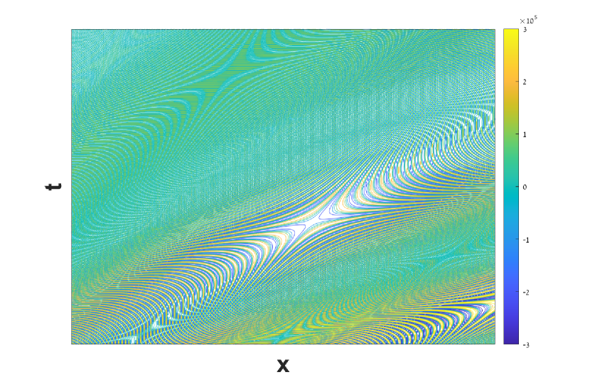
Figure 2: Zoom of a part of the region in Fig. 1, where $x/x_{0}\in[1.5\,,2]$ and $t\in[4\cdot 10^{-5}\,,7\cdot 10^{-5}]$. More details are shown with smaller cells of the grid: $\Delta x=2\cdot 10^{-6}$ and $\Delta t=5\cdot 10^{-8}$

7 Conclusion

Two examples of quantum dynamics is considered in the form of quantum counterparts of turbulent diffusion in comb geometry. The latter is described by either Langevin equation in the Matheron - de Marsily form of Eq. (1.1) or equivalently by the Fokker-Planck equation (FPE) in the form of the 2D comb model (1.2). The solution of the latter form corresponds to the log-normal-Lévy-Smirnov density of the random variable $x$ with the variance growing exponentially: $\mathrm{var}(x)=\langle(x-\langle x\rangle)^{2}\rangle\sim e^{t}$, It describes relative diffusion of a pair of particles, namely the distance between them. Therefore one finds that the relative diffusivity of any two particles grows with the inter-particle distance; and due to this growth, this process has a property of turbulent diffusion.

Having concerned with the quantum dynamics, we have constructed two variants of continuous time quantum walks related to non-Hermitian operators of the form $\hat{{\cal H}}=\hat{A}+i\hat{B}$, where $\hat{A}$ is responsible for the unitary transformation, while $i\hat{B}$ is responsible for quantum/classical relaxation. The first model in Eq. (4.1) is obtained by multiplication of the comb model by $\hbar\sqrt{-1}$. As a rule, such simple multiplication of an equation by a constant does not lead to a new solution. However, due to the forms of the classical advection $x\partial_{x}$ and the dilatation operator $\hat{{\cal H}}_{0}=-i\hbar(x\partial_{x}+1/2)=\hat{A}$, one immediately arrives at non-Hamiltonian quantum mechanics inside the backbone, which leads to quantum effects. In particular, it is quantum tunneling inside a dead zone, which is a quantum swimming upstream, that is a quantum initial wave packet moves against the classical streaming. The fingers play a role of classical environment with classical relaxation according to normal diffusion.

The second model corresponds to a standard quantum counterpart of a classical FPE by the Wick rotation of time $t\rightarrow it$. The unitary dynamics inside fingers is due to free motion, $\hat{A}=\frac{\hbar^{2}}{2}\partial_{y}^{2}$. The relaxation is due to the dilatation operator $\hat{B}=\hat{{\cal H}}_{0}\delta(y)$, which is an imaginary optic scattering potential for the incident plain wave coming from the fingers. It is also a trap, which violets the optical theorem.

In conclusion, we comment symmetrical-asymmetrical positioning of the initial conditions, which is a generic task related to the comb geometry for both quantum mechanics and classical diffusion. To be specific, let us consider the initial condition for Eq. (1.2) in a finger with $y=y_{0}\neq 0$ with the initial PDF $P_{0}(x,y)=\delta(x-x_{0})\delta(y-y_{0})$. Then, following Eq. (2.3) with $g(y,s)=e^{-|y|\sqrt{s/D}}$, the finger transport is started first with the Lévy-Smirnov density (2.10), $P_{y}(y-y_{0},t)=\tfrac{|y-y_{0}|}{\sqrt{4D\pi t^{3}}}e^{-\frac{(y-y_{0})^{2}}{4Dt}}$, which is also a first arrival time distribution to the backbone [29]. Then, in the backbone’s transport equation, the Lévy-Smirnov distribution $P_{y}(y_{0},t)$ plays a role of a strength of a $\delta$ source - sink term at $x=x_{0}$. This situation differs from both scenarios considered above and has been discussed for anomalous diffusion and random search in two and three dimensional combs [30, 31].

Appendix A Imaginary optical potential vs optical theorem

The optical theorem, results from the conservation of the probability flux at elastic scattering and establish the relation between a scattering cross section and a scattering amplitude, and it also relates to the interference between incident and scattered waves [18]. Some general aspects of the one dimensional scattering, including the optical theorem, have been considered as well [32]. To understand the violation of the optical theorem by scattering at imaginary optical potential $i\delta(y)$, we first consider Eq. (6.5) for the real attractive delta potential [25, 27], which reads

$$-\frac{\hbar^{2}}{2}\partial_{y}^{2}\Phi_{e}-\lambda\delta(y)\Phi_{e}=e\Phi_{e}\,.$$ (A.1)

The scattering solutions (6.6) for the left and right incident waves are

$$\Phi^{\pm}_{k}(y)=\frac{1}{\sqrt{2\pi}}\left[e^{\pm iky}+\mathcal{B}(k)e^{ik\lvert y\rvert}\right],$$ (A.2)

where the scattering amplitude and the energy are

$$\mathcal{B}(k)=\frac{-\lambda}{(\lambda-i\hbar^{2}k)}\,,\quad\quad e=e(k)=\hbar^{2}k^{2}/2\,.$$ (A.3)

Let us consider the flux, specifically for the left incident wave $\psi_{k}(y)=\Phi^{+}_{k}(y)$ it reads

$$\frac{J_{k}(y)}{\hbar k}=\frac{1}{2i}\left[\psi_{k}^{*}\partial_{y}\psi_{k}-\psi_{k}\partial_{y}\psi_{k}^{*}\right]=1-\frac{\lambda(1+\rm{sgn}(y))e^{ik(|y|-y)}}{2(\lambda-i\hbar^{2}k)}\\ -\frac{\lambda(1+\rm{sgn}(y))e^{-ik(|y|-y)}}{2(\lambda+i\hbar^{2}k)}+\frac{\lambda^{2}\rm{sgn}(y)}{|\lambda+i\hbar^{2}k|^{2}}]=\\ =1+(1+\rm{sgn}(y))\rm{Re}\mathcal{B}(k)\cos[k(|y|-y)]+\left|\mathcal{B}(k)\right|^{2}\rm{sgn}(y)\,,$$ (A.4)

where $(1+\rm{sgn}(y))\sin[k(|y|-y)]\equiv 0$ and $\rm{Re}\mathcal{B}(k)=-\left|\mathcal{B}(k)\right|^{2}$. The letter expression is nothing more as an analog of the optical theorem relevant for the one dimensional scattering [32].

Note that the scattering amplitude $\mathcal{B}(k)$ in the solution (A.2) determines the reflection and transmission coefficients. Namely, for $y<0$, the reflection coefficient is ${\cal R}=\mathcal{B}(k)$, while the transmission coefficient for $y>0$ is ${\cal T}=1-{\cal B}$. This immediately yields the law of conservation of the number of particles, $|{\cal T}|^{2}+|{\cal R}|^{2}=1$. From Eq. (A.4), also follows that $J_{k}(y>0)=J_{k}(y<0)=\hbar k-\hbar k\left|\mathcal{B}(k)\right|^{2}$.

Now let us consider the current for the scattering at the imaginary optical potential $i\delta(y)$. From the solution (6.6) with $\mathcal{B}(k)={\lambda}/{(\hbar^{2}k-\lambda)}$, we have that now the scattering amplitude does not correspond to the optical theorem and does not describes the reflection and transmission coefficient. Namely $|{\cal T}|^{2}+|{\cal R}|^{2}=1+\frac{2\lambda\hbar^{2}k}{(\lambda-\hbar^{2}k)^{2}}$ and it violets the law of conservation of the number of particles. Therefore, the imaginary optical potential $i\delta(y)$ relates to the scattering with violation of the optical theorem.

References

References

• [1] G. Matheron, G. de Marsily, Is transport in porous media always diffusive? a counterexample, Water Resour. Res. 16: 901 - 917, (1980).
• [2] E. Baskin, A. Iomin, Superdiffusion on a comb structure, Phys. Rev. Lett. 93: 120603, 2004.
• [3] M.V. Berry, J.P. Keating, $H=xp$ and the Riemann zeros, in: J.P. Keating, D.E. Khmelnitskii, I.V. Lerner (Eds.), Supersymmetry and Trace Formulae: Chaos and Disorder, Kluwer, New York, 1999.
• [4] M.V. Berry, J.P. Keating, The Riemann zeros and eigenvalue asymptotics, SIAM Rev. 41(2): 236 - 266, 1999.
• [5] A. Connes, Trace formula in noncommutative geometry and the zeros of the Riemann zeta function, Selecta Math. New Ser. 5: 29, 1999; math.NT/9811068.
• [6] G. Sierra, $H=xp$ with interaction and the Riemann zeros, Nucl. Phys. B 776 [PM]: 327 - 364, 2007.
• [7] V. de Alfaro, S. Fubini, and G. Furlan, Conformal invariance in quantum mechanics, Nuovo Cimento A 34: 569 - 612, 1976.
• [8] R. Jackiw, in M. A. B. Beg Memorial Volume ed A. Ali and P. Hoodbhoy, World Scientific, Singapore, 1991
• [9] C. van Winter, An increasing entropy for a free quantum particle, J. Math. Phys. 39: 3600 - 3618, 1998.
• [10] J. V. Armitage, The Riemann hypothesis and the Hamiltonian of a quantum mechanical system, in Number Theory and Dynamical Systems, edited by M. M. Dodson and J. A. G. Vickers, Cambridge University Press, Cambridge, UK, 1989.
• [11] J. Twamley, G. J. Milburn, The quantum Mellin transform, New J. Phys. 8: 328, (2006).
• [12] R. K. Bhaduri, A. Khare, and J. Law, Phase of the Riemann zeta function and the inverted harmonic oscillator, Phys. Rev. E 52: 486 - 491, 1995.
• [13] S. Nonnenmacher and A. Voros, Eigenstate structures around a hyperbolic point, J. Phys. A 30: 295 - 315, 1997.
• [14] G. P. Berman and M. Vishik, Long time evolution of quantum averages near stationary points, Phys. Lett. A 319: 352 - 359, 2003.
• [15] A. Iomin, Exponential spreading and singular behavior of quantum dynamics near hyperbolic points, Phys. Rev. E 87: 054901, 2013.
• [16] A. Iomin, Fractional-time quantum dynamics, Phys. Rev. E 80: 022103, 2009.
• [17] T. Sandev, A. Iomin, and L. Kocarev, Hitting times in turbulent diffusion due to multiplicative noise, upublished 2020.
• [18] A. M. Perelomov and Y. B. Zel’dovich, Quantum Mechanics - Selected Topics, WS, Singapore, 1998.
• [19] P. L. Krapivsky, J. M. Luck, and K. Mallick, Survival of classical and quantum particles in the presence of traps, J. Stat. Phys. 154: 1430 - 1460, 2014.
• [20] R. N. Deb, A. Khare, and B. D. Roy, Complex optical potentials and pseudo-Hermitian Hamiltonians, Phys. Lett. A 307: 215 - 221, 2003.
• [21] V. A. Fock, Foundations of Quantum Mechanics, Nauka, Moscow, 1976 (in Russian).
• [22] L. D. Landau, E. M. Lifshitz, Quantum Mechanics, Pergamon, New York, 1977.
• [23] H. Bateman and A. Erdélyi, Higher Transcendental Functions, [V. 1 – 3], McGraw-Hill, New York, 1953–1955.
• [24] A. M. Mathai and H. J. Haubold, Special Functions for Applied Scientists, Springer, NY, 2008.
• [25] A. Iomin, V. Mendez, and W. Horsthemke, Fractional Dynamics in Comb-like Structures WS, Singapore, 2018.
• [26] E. Agliary, O. Mülken, and A. Blumen, Continuous-time quantum walks and trapping, Int. J. of Bif. 20; 271 - 279, 2010.
• [27] S. M. Blinder, Green’s function and propagator for the one-dimensional $\delta$-function potential, Phys. Rev. A 37: 973 - 976, 1988.
• [28] H. Bateman and A. Erdélyi, Tables of integral transforms, [V. 1], McGraw-Hill, New York, 1954.
• [29] T. Sandev, A. Iomin, and L. Kocarev, Random search on comb, J. Phys. A: Math. Theor. 52: 465001, 2019.
• [30] A. Iomin and T. Sandev, Fractional diffusion to a Cantor set in 2D, unpublished.
• [31] E. K. Lenzi, T. Sandev, H. V. Ribeiro, P. Jovanovski, A. Iomin, and L. Kocarev, Anomalous diffusion and random search in xyz-comb: exact results, J. Stat. Mech. 2020: 053203, 2020.
• [32] J. H. Eberly, Quantum scattering theory in one dimension, Am. J. Phys. 33: 771 - 773, 1965.