Rotational spectra of vibrationally excited AlO and TiO in oxygen rich stars

Abstract

Rotational transitions in vibrationally excited AlO and TiO — two possible precursors of dust — were observed in the 300 GHz range (1 mm wavelength) towards the oxygen rich AGB stars R Dor and IK Tau with ALMA, and vibrationally excited AlO was observed towards the red supergiant VY CMa with the SMA. The $J=11\to 10$ transition of TiO in the $v=1~{}{\rm{and}}~{}2$ levels, and the $N=9\to 8$ transition in the $v=2$ level of AlO were identified towards R Dor; the $J=11\to 10$ line of TiO was identified in the $v=1$ level towards IK Tau; and two transitions in the $v=1~{}{\rm{and}}~{}2$ levels of AlO were identified towards VY CMa. The newly-derived high vibrational temperature of TiO and AlO in R Dor of $1800\pm 200$ K, and prior measurements of the angular extent confirm that the majority of the emission is from a region within $\lesssim$2 $R_{\star}$ of the central star. A full radiative transfer analysis of AlO in R Dor yielded a fractional abundance of $\sim$3% of the solar abundance of Al. From a similar analysis of TiO a fractional abundance of $\sim 78$% of the solar abundance of Ti was found. The observations provide indirect evidence that TiO is present in a rotating disk close to the star. Further observations in the ground and excited vibrational levels are needed to determine whether AlO, TiO, and TiO₂ are seeds of the Al₂O₃ dust in R Dor, and perhaps in the gravitationally bound dust shells in other AGB stars with low mass loss rates.

1 Introduction

Most low and intermediate mass stars ($\sim 0.8$–$8~{}\mathrm{M}_{\odot}$) pass through the asymptotic giant branch (AGB) phase after leaving the main sequence and exhausting the hydrogen and helium in their cores. High-mass stars ($\gtrsim 8~{}\mathrm{M}_{\odot}$), however, pass through the similarly cool red super giant (RSG) phase while fusing helium. Both AGB and RSG stars have high mass-loss rates and produce a significant amount of dust in their molecule rich stellar winds. For a comprehensive review of AGB and RSG stars, see Höfner & Olofsson (2018) and Levesque (2017).

The precise formation pathways of dust in AGB and RSG stars are not yet known, but in the past few years astronomers have begun observing rotational lines of a few small metal bearing molecules which might be the precursors of the dust. The high sensitivity and angular resolution of interferometers such as the Atacama Large Millimeter/submillimeter Array (ALMA) have allowed astronomers to compare the abundance distributions of small gaseous molecules with the infrared emission from the dust, and to consider the possible connection between the gaseous molecules and the dust formation and growth process within a few stellar radii ($R_{\star}$) of the central star (Kamiński, 2019).

Optical and near-infrared polarimetric images of the dust do not directly reveal the composition and processes by which the dust is formed (Khouri et al., 2016; Ohnaka et al., 2016), but parallel studies of the abundance distributions of the gas phase molecules in the dust forming region might help unravel the physicochemical processes that occur in the phase change from small molecules to gas phase clusters and ultimately tiny dust grains. Karovicova et al. (2013) used infrared interferometric observations from VLTI/MIDI (the MID-infrared Interferometric instrument on the VLT interferometer) to show that two oxygen rich Mira stars with low mass loss rates (S Ori and R Cnc) are surrounded by an amorphous Al₂O₃ shell at $\sim$2 stellar radii; while an AGB star with a high mass loss rate (GX Mon) is surrounded by an Al₂O₃ dust shell at around 2 stellar radii and a silicate layer around 4 stellar radii. This led Karovicova et al. to hypothesise that stars with low mass loss rates primarily form dust whose spectral properties match Al₂O₃, and stars with higher mass loss rate form dust with the spectral properties of warm silicates.

In oxygen rich AGB and RSG stars (the focus of the work here), the most accessible metal oxides and hydroxides in the millimeter band are SiO, AlO, AlOH, TiO, and TiO₂. SiO has been extensively studied since the early days of millimetre astronomy (see for example González Delgado et al., 2003), and several studies have been devoted to AlO, owing to its relatively intense lines in the millimeter band and the possible correlation with the infrared emission from alumina (Al₂O₃) in the dust forming region (e.g. Tenenbaum & Ziurys, 2009; Kamiński et al., 2016; Decin et al., 2017). But at present it is not yet known for certain which metal oxides and hydroxides are the initial building blocks of the identified dust species.

Rotational lines of AlO were first detected in the red supergiant VY CMa with the Arizona Radio Observatory (ARO) 10 m antenna by Tenenbaum & Ziurys (2009); and subsequently observed in an interferometric spectral line survey of VY CMa with the Submillimeter Array (SMA) (Kamiński et al., 2013b); and in Mira ($o$ Cet, Kamiński et al., 2016), W Hya (Takigawa et al., 2017), and R Dor and IK Tau with ALMA (Decin et al., 2017).

A major contribution toward elucidating the connection of AlO and the dust is the comprehensive study of the Al content in R Dor by Decin et al. (2017). They concluded that the principal small gaseous precursors of aluminum grains (AlO, AlOH, and AlCl) are: (1) observed both in and beyond the dust formation region, (2) account for only a small fraction of the aluminum budget, and (3) condensation of small gaseous aluminum bearing molecules is not 100% efficient.

Parallel to the work on AlO, rotational lines of TiO and TiO₂ were observed with low peak flux in VY CMa in the same spectral line survey with the SMA (Kamiński et al., 2013b, a). Subsequently TiO₂ was observed with much higher sensitivity and angular resolution in VY CMa with ALMA by De Beck et al. (2015), who concluded TiO₂ is not a tracer for “low grain formation efficiency” in the complex source VY CMa, because the emission extends well beyond the dust condensation radius.

Both TiO and TiO₂ were also observed with ALMA in three nearby AGB stars: Mira A (the AGB component of a binary, Kamiński et al., 2017), and R Dor and IK Tau (Decin et al., 2018). Kamiński et al. (2017) concluded on the basis of the observations of TiO and TiO₂ and indirect chemical arguments, that it is unlikely that substantial amounts of Ti are locked up in solids in Mira A because: (1) the abundance of gaseous titanium species is very high; (2) a gas phase chemical model is in general agreement with the measured abundances of TiO and TiO₂ in the millimeter band (Gobrecht et al., 2016); and (3) TiO₂ emission extends $5.5\,R_{\star}$ from Mira A, rather than close to the star where the temperature is higher and inorganic dust is expected to form. However Khouri et al. (2018) estimated 80% of the expected Ti in Mira A is either in the atomic form or in the dust grains on the basis of: (1) a full radiative transfer analysis of CO close to the star and a radiative transfer analysis of dust; (2) an LTE analysis of TiO₂ in the ground vibrational state; and (3) the relative abundance of TiO and TiO₂ derived by Kamiński et al. (2017).

There is a general consensus that additional observations with ALMA of AlO, AlOH, TiO, TiO₂, and other metal oxides and hydroxides are needed to establish more stringent constraints on the dynamical chemical models of the inner winds of oxygen rich AGB and RSG stars. Conclusive evidence for a strong spatial correlation with the onset of the dust condensation in the inner wind of oxygen rich stars can only be made in a credible way if accurate abundance structures of AlO, TiO, TiO₂, etc are retrieved from rotational spectra observed at high sensitivity and angular resolution — i.e., astronomers cannot simply rely on the apparent correlation of millimeter-wave rotational line emission and IR dust emission close to the central star. As previous observations of AlO in the ground vibrational state have shown (Kamiński et al., 2016; Decin et al., 2017), gaseous AlO and AlOH are observed beyond the dust condensation zone, but these two principal small aluminum bearing molecules and AlCl only consume $\sim$2% of the total Al budget. Hence, there is ample room left for other Al bearing dust species (or larger gas-phase clusters) to form, and the same might hold for TiO and TiO₂. Instead what is needed is a proper assessment of the total Ti consumed in the gas phase species, and whether other explanations — e.g., unresolved complex density structures close to the central star — can be ruled out.

With the aim of advancing the observations of the metal oxides we examined existing interferometric spectral line surveys of two AGB stars (R Dor and IK Tau) and the RSG star VY CMa for evidence of vibrationally excited AlO and TiO (Sect. 3). However, owing to subtleties in the rotational spectrum of vibrationally excited AlO, and the sparsity of direct laboratory measurements of rotational transitions in vibrationally excited TiO, we first reviewed the pertinent molecular physics of these two open shell molecules (Sect. 2). The identification of millimeter-wave rotational lines of vibrationally excited AlO in three stars (VY CMa, R Dor, and IK Tau), and vibrationally excited TiO in two of these (R Dor, and IK Tau) is described in Sect. 3. This is followed by a full radiative transfer analysis of the rotational lines of AlO and TiO in R Dor (Sect. 4), from which abundance distributions were derived from observational data of AlO (Sects. 4.3) and TiO (Sect. 4.4). In Sect. 5 we critically considered the evidence for whether TiO (and by inference TiO₂) are seeds of the Al₂O₃ dust in the gravitationally bound dust shell (GBDS) of R Dor.

In the work here we have adhered to the description of R Dor in the recent papers by Khouri et al. (2016); Van de Sande et al. (2018), and Decin et al. (2017, 2018). The semiregular (SR) variable oxygen rich star R Dor is the closest AGB star to our Sun (59 pc, Knapp et al., 2003). It has a very low mass loss rate ($1.6\times 10^{-7}\,\;\mathrm{M}_{\odot}~{}\mathrm{yr}^{-1}$, Maercker et al., 2016), the stellar diameter is large (54 mas, Norris et al., 2012), it is molecule rich, and there is a 27 GHz wide spectral line survey in Band 7 with ALMA (Decin et al., 2018) in which 22 molecules and isotopologues have been identified. It has been shown from polarized dust emission, at high angular resolution in the optical and near IR, that there is a high density dust envelope — or gravitationally bound dust shell (GBDS) — in R Dor that is close to the star (Khouri et al., 2016, and references therein). Modelling such a shell is needed to account for the infrared emission from amorphous Al₂O₃ and the fractions of scattered light seen towards low mass-loss rate stars such as R Dor and W Hya (Khouri et al., 2015). The GBDS around R Dor is located within $1.7-1.9\,R_{\star}$ (Khouri et al., 2016) and is thought to consist of amorphous Al₂O₃ grains or Fe-free silicates with a preference towards Al₂O₃, because Al₂O₃ can condense at higher temperatures. The stellar wind is launched from the outer edge of the GBDS (Van de Sande et al., 2018, and references therein). The focus here is on the inner wind region within 300 mas of the central star that includes most of the AlO and TiO emission (Decin et al., 2017, 2018), and especially the region within the dust condensation radius at $\lesssim$ (2-3) $R_{\star}$ of the central star (Van de Sande et al., 2018).

2 Molecular physics of vibrationally excited AlO and TiO

2.1 AlO

The millimeter-wave rotational spectra of AlO were directly measured in the laboratory in the $v=1$ and $v=2$ levels (Goto et al., 1994) and are tabulated in Launila & Banerjee (2009) and CDMS. The spectroscopic constants in the higher vibrational levels ($v=3,\cdots,7$) of AlO were derived from rotationally resolved spectra of the two lowest electronic transitions ($A^{2}\Pi\rightarrow X^{2}\Sigma$ and $B^{2}\Sigma\rightarrow X^{2}\Sigma$; Launila & Berg, 2011). Rotational transitions in the higher vibrational levels with $v\geq 3$ calculated with the constants of Launila & Berg (2011) should be sufficiently accurate for unambiguous identification in the frequency band in which lines of ground state AlO have been observed.

The rotational lines of AlO in the ground vibrational state are especially wide compared with other molecules such as CO and SiO, whose lines are primarily broadened by the Doppler effect, owing to the expanding envelopes in which they are observed. The large observed line widths of AlO are a consequence of the molecular physics: the nuclear spin ($I$) of ²⁷Al is 5/2; the Fermi contact magnetic hyperfine constant ($b_{F}$) is especially large; and the spin-rotation interaction ($\gamma$) in the $X^{2}\Sigma$ electronic ground state causes the hyperfine structure to appear as two partially overlapping patterns of 5 to 7 hyperfine split components, whose centroids are split by approximately $\gamma$.

In most diatomic molecules $\gamma$ changes very little in successive vibrational levels. However, owing to a second order interaction of the $X^{2}\Sigma$ electronic ground state of AlO with the low lying $A^{2}\Pi$ excited state (7775 K above ground, Ito & Goto, 1994), the magnitude of $\gamma$ changes from one vibrational level to the next such that in the ground ($v=0$) vibrational state ($\gamma=51.66$ MHz, Goto et al., 1994) $\gamma$ is about 3 times larger than in the $v=1$ level ($\gamma=15.95$ MHz, Goto et al., 1994); $\gamma$ changes sign between the $v=1$ and $v=2$ levels, and the magnitude is 1.6 times larger in the $v=2$ than the $v=1$ level ($\gamma=-31.467$ MHz, Goto et al., 1994); and the magnitude of $\gamma$ is 3.3 times larger in the $v=3$ level than the $v=2$ level ($\gamma=-103.43$ MHz, Launila & Berg, 2011). Therefore the rotational lines in the $v=1$ level are much narrower than in ground state, but lines in the $v=3$ level are predicted to be very broad and might be difficult to detect. Because the widths of the rotational lines of AlO vary so markedly from one vibrational level to the next, they provide an independent spectroscopic confirmation of the assignments.

2.2 TiO

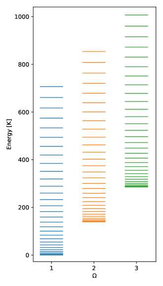
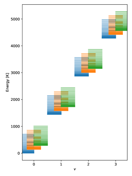
Figure 1: Energy level diagram of TiO in the $X^{3}\Delta_{\Omega}$ ground electronic state calculated with effective spectroscopic constants (see Table 2 in Ram et al., 1999). Left: The rotational levels with $J\leq 30$ in the ground ($v=0$) vibrational state of the three fine structure components ($\Omega=1,2,~{}{\rm{and}}~{}3$). Right: Rotational levels with $J\leq 30$ in the ground and three lowest excited vibrational levels with the same color coding for $\Omega$ as in the panel on the left.

The pure rotational spectrum of TiO in the ground $X^{3}\Delta$ electronic state was measured directly in the ground vibrational state (Namiki et al., 1998; Steimle & Virgo, 2003; Breier et al., 2019), and recently two transitions in the first excited vibrational level were also measured by (Breier et al., 2019). Namiki et al. (1998) measured 12 rotational transitions of TiO between the $J=6~{}{\rm{and}}~{}14$ levels in the $220-460$ GHz range in a large absorption cell, and the two lowest transitions at 63 and 95 GHz by microwave optical double resonance; from these Namiki et al. derived the leading spectroscopic constants of TiO in the $X^{3}\Delta_{i}$ electronic ground state. The same group subsequently measured the permanent electric dipole moment ($\mu$) of the $X^{3}\Delta$ state in the optical Stark spectrum of three electronic transitions (Steimle & Virgo, 2003). More recently Breier et al. (2019) accurately measured 14 rotational transitions of TiO between 253 and 384 GHz with a $1\sigma$ measurement uncertainty of 50 kHz in the ground vibrational state, and two transitions in the $v=1$ level of the ${}^{3}\Delta_{2}$ spin-orbit component in absorption (at 286.5 and 318.3 GHz with an uncertainty of 100 kHz) in a supersonic molecular beam.

The most comprehensive spectroscopic analysis of the rotational spectrum of TiO was by Ram et al. (1999), who derived the rotational and fine structure constants in the four lowest excited vibrational levels ($v=1,\cdots,4$) from a combined analysis of rotationally resolved spectra of the $A^{3}\Phi\to X^{3}\Delta$ electronic transition near $1~{}\micron$ in the laboratory and in a sunspot, and of the direct measurements in the ground vibrational state. The TiO molecule in its $X^{3}\Delta_{\Omega}$ ground electronic state is a good Hund’s case $(a)$ molecule with electron spin angular momentum ($\Sigma$) of 1; orbital angular momentum ($\Lambda$) of 2; $\Omega=|{\Lambda+\Sigma}|$, where, by vector addition, $\Omega$ has the possible values of 1, 2, and 3; and the rotational levels have integral values with $J\geq\Omega$. Because the spin-orbit constant ($A$) is positive, the $X^{3}\Delta_{1}$ spin orbit component is lowest in energy followed by the $X^{3}\Delta_{2}$, and $X^{3}\Delta_{3}$ components with relative energies of about 140 K between components (see Fig. 1). The three spin components are metastable, because $A$ is much greater than the rotational constant $B$, and as a result the line strengths for cross ladder ($\Delta\Omega=\pm 1$) transitions are very small.

3 Astronomical Observations

Many unidentified (U) lines have been observed in spectral line surveys of AGB stars, suggesting the identification of new species might be within reach. When we considered possible carriers of the U lines, for example towards the oxygen rich stars VY CMa, R Dor and IK Tau (Kamiński et al., 2013a; Decin et al., 2018), we realized rotational lines of vibrationally excited AlO and TiO should be readily identifiable for three reasons. First, the lowest vibrational levels of both molecules will be populated in the inner wind, because the vibrational frequencies of AlO (1389 K) and TiO (1438 K) are comparable to the kinetic temperature of the gas ($T_{\rm{gas}}$) within a few stellar radii of the star (see for example Eq. 1 in Sect. 4.2.2). Second, a wealth of supporting laboratory spectroscopy for both molecules has been published as summarized in Sects. 2.1 and 2.2. And finally, the peak fluxes of the ground state lines in sensitive interferometric spectra are high enough so lines in the lowest few excited vibrational levels should be observable in existing surveys.

3.1 VY CMa

Figure 2: Two successive rotational transitions of AlO observed with a $1^{\prime\prime}$ beam in VY CMa with the SMA (Kamiński et al., 2013a). The transition quantum numbers are indicated in the top left of each box. Data are plotted as red histograms, the unresolved fine and hyperfine structure is indicated by the vertical lines in green, and theoretical Gaussian profiles from least squares fits to the observed spectra are plotted in blue. In the $v=2$ level the full composite synthetic profile with hyperfine structure is plotted, because the spectra were too noisy to analyze with a theoretical Gaussian profile.

Table 1: AlO in VY CMa Observed with the SMA

$N^{\prime}\to N$	$v$	$\nu_{\rm{calc}}$	$\nu_{\rm{obs}}$	Peak Flux	$\Delta\upsilon$	$\upsilon_{\rm{LSR}}$	Beam		Int. Flux	Line width
		(MHz)	(MHz)	(mJy)	(km s-1)	(km s-1)	(″)		(Jy km s-1)	ratio
$8\to 7$	0	306,197.319	306,172.3 $\pm$ 0.8	580	53.8 $\pm$ 2.0	24.5 $\pm$ 0.8	0.91		32.4 $\pm$ 1.6	1.0
	1	303,412.064	303,390.0 $\pm$ 0.6	477	17.5 $\pm$ 1.5	21.8 $\pm$ 0.6	0.91		8.9 $\pm$ 0.9	$3.1\pm 0.3$
	2	300,611.392	c300,591.0 $\pm$ 3.0	340	41.0 $\pm$ 7.2	20.3 $\pm$ 3.0	0.92		7.7 $\pm$ 1.6	$1.3\pm 0.2$
$9\to 8$	0	344,451.721	344,423.4 $\pm$ 0.3	1040	45.8 $\pm$ 0.7	24.6 $\pm$ 0.3	0.88		50.8 $\pm$ 1.0	1.0
	1	341,318.153	341,294.6 $\pm$ 0.6	661	12.6 $\pm$ 1.1	20.7 $\pm$ 0.5	0.82		12.5 $\pm$ 1.1	$3.6\pm 0.3$
	2	338,167.232	c338,141.0 $\pm$ 1.0	242	24.2 $\pm$ 2.1	23.3 $\pm$ 0.9	0.81		6.2 $\pm$ 0.7	$1.9\pm 0.2$

We began by searching for vibrationally excited AlO in the spectral line survey of VY CMa in the $279.5-355$ GHz range observed with the eight element SMA at a modest sensitivity and angular resolution ($\sim$1^′′; Kamiński et al., 2013a). The initial identifications of vibrationally excited AlO were made on the basis of the calculated rotational frequencies in the three lowest excited vibrational levels ($v\leq 3$) in the absence of fine and hyperfine structure (i.e., with $\gamma,b_{F}$, the dipole-dipole magnetic hyperfine constant $c$, and the electric quadrupole coupling constant $eQq$ constrained to zero). Although the frequencies of the rotational transitions of AlO calculated with only two spectroscopic constants (the rotational constant $B$ and centrifugal distortion constant $D$) are approximate, the centroids of the synthetic line profiles reproduce the astronomical features to within a few MHz and are sufficient for establishing the identification of lines of vibrationally excited AlO in the astronomical spectra. The frequencies and relative intensities of the hyperfine components used to calculate the synthetic profiles of AlO in the $v=0,1,\,{\rm{and}}~{}2$ levels are tabulated in (Launila & Banerjee, 2009). The term energy for the $v=1$ excited vibrational level is 1389 K and 2758 K for the $v=2$ level.

Two successive rotational transitions of AlO in the ground vibrational state ($N=8\to 7$ at 306 GHz, and $N=9\to 8$ at 344 GHz) were covered in the SMA survey, and both were also observed in vibrationally excited levels: the $v=1$ and possibly the $v=2$ level in the $N=8\to 7$ transition, and $v=1$ and $v=2$ levels in the $N=9\to 8$ transition (see Fig. 2 and Table 1). The line parameters for most measurements were derived by fitting Gaussian profiles to the astronomical features. All measurements were done on spectra obtained from the central pixel of the SMA data, corresponding to a restoring beam of $\sim 1\arcsec$ centred on the continuum peak of VY CMa (for precise beam sizes at different frequencies, see Kamiński et al., 2013a). The observed frequencies $\nu_{\rm{obs}}$ in the ground vibrational state and the $v=1$ level and the FWHM line width, $\Delta v$, were derived from Gaussian profiles that were least squares fit to the spectra (see Fig. 2). The synthetic profiles of the lines in the $v=2$ vibrational state were obtained by representing each hyperfine component with a Gaussian profile whose HWHM was 2.5 km s^-1. The relative intensities of the hyperfine components were equivalent to the theoretical relative intensities in Launila & Banerjee (2009). The variables in the least squares fit of the synthetic profile to the observed profile were: an intensity (scaling) factor of the composite theoretical synthetic profile and the center frequency. The mean central LSR velocity $\upsilon_{\mathrm{LSR}}=21.5\pm 3.3$ km s^-1 for the four rotational transitions in the excited vibrational levels of AlO in Table 1 is in good agreement with the stellar velocity ($v_{\mathrm{LSR}}=22$ km s^-1, Kamiński et al., 2013a) and the LSR velocity of AlO in the ground vibrational state ($\upsilon_{\mathrm{LSR}}=25\pm 2$ km s^-1) observed with the SMA in VY CMa by Kamiński et al. (2013a), confirming the assignment of the new lines of vibrationally excited AlO. As expected, the FWHM of the lines are $3.3\pm 0.4$ times smaller in the $v=1$ level, and $1.6\pm 0.3$ times smaller in the $v=2$ level than those in the ground vibrational state — i.e., close to the theoretical predictions discussed in Sect. 2.1, thereby providing further confirmation of the line assignments. The rotational lines in the $v=3$ vibrational level were not observed because the predicted peak flux is comparable to the peak noise in the spectra shown in Fig. 2. The details of the detected lines are given in Table 1.

3.2 R Dor and IK Tau

Table 2: Details of ALMA observations of AlO and TiO towards R Dor and IK Tau.

Transition	Freq	Proposal	Date(s)	ToS	PWV			Synth. beam	Vel. res.	rms	MRS
	(GHz)		(yyyymmdd)	(min)	(mm)			(mas,mas,deg)	(km s-1)	(mJy)	(arcsec)
R Dor
AlO $N=6\to 5$	229.670	2017.1.00824.S	20171024–	192	0.6			33, 29, +55	0.32	0.8	2.6
			20171026
AlO $N=7\to 6$	267.937	2017.1.00824.S	20171231–	165	1.2			138,131,$-55$	0.273	1.0	5.0
			20180105
AlO $N=8\to 7$	306.197	2017.A.00012.S	20181211	6.5	0.9			110, 88, $-45$	0.911	3.8	3.1
AlO $N=9\to 8$	338.167–	2013.1.00166.S	20150827–	25.2	0.3–			165, 127, $+29$	0.9–	3.5–	3.1
& TiO lines	355.623		20150901		0.7			150, 125, $+21$	0.8	4.5
IK Tau
AlO $N=9\to 8$	338.167–	2013.1.00166.S	20150813–	10	0.2–			175, 145,$-15$	1.7–	4.7–	3.1
& TiO lines	355.623		20150828		1.7			165, 135,$-10$	1.6	5.3

The data used in this paper were taken from the ALMA projects with codes and other observing details given in Table 2; see the ALMA Science Archive for more details. The raw data were calibrated using standard ALMA procedures including application of instrumental calibration and corrections derived from the bandpass and phase reference sources. The flux scale is in most cases accurate to 7% or better; however, for AlO $N=6\to 5$ the phase reference source flux density fluctuated by 12% over the observations, which is probably bona fide variability but gives an upper bound to the uncertainty for these data. Decin et al. (2018) gives details of the data reduction for 2013.1.00166.S and we followed a similar route in all cases. In brief, line-free channels were identified and used for self-calibration of the strong continuum emission from the star (and potentially hot dust). After applying all calibration to the line data, spectral cubes were made at the resolutions and sensitivities given in Table 2, averaging where necessary to improve surface brightness sensitivity.

The continuum was unresolved or barely resolved, with a flux density ranging from 252 mJy in the image covering AlO $N=6\to 5$, to 596 mJy covering AlO $N=9\to 8$. The relative astrometry between continuum and line in the same data-set is limited by the synthesised beam/signal-to-noise ratio (S/N). This is $<1$ mas for all continuum images. For the moment maps, the relative position uncertainty is $\sim$5 mas for the weakest emission, down to $<1$ mas for the brightest — less than a pixel in all cases.

We extracted spectra in an aperture of 150 mas radius for AlO and 300 mas for TiO towards R Dor and in an aperture of 320 mas for AlO or 160 mas for TiO for IK Tau. The peak and integrated fluxes given in Tables 3 and 4 were measured from these spectra. We made zeroth-order moments (integrated flux density) over the channels where the line signal exceeded the rms. For the cases where lines participate in overlaps with lines of other species, the details are discussed in Sections 3.2.1 and 3.2.2 for AlO and TiO, respectively. Due to the quality and quantity of data, we mostly focus on R Dor for our analysis.

3.2.1 AlO

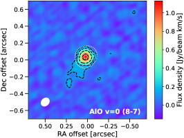
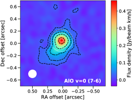
Figure 3: For R Dor: zeroth moment maps of rotational transitions of AlO in the ground ($X^{2}\Sigma$) electronic state, observed with ALMA. Left: $N=9\to 8$ in the $v=2$ vibrational state. Centre: $N=8\to 7$ in the ground vibrational state. Right: $N=7\to 6$ in the ground vibrational state. The black dashed contours indicate flux levels at 3, 6, 12… times the off-source noise rms for AlO. The synthesized beams are indicated by ellipses in the lower left corner of each panel. The dotted white contours are at levels of 1, 10, and 90% of the peak continuum flux and are included to indicate the position of the star.

Table 3: The observed transitions of AlO towards R Dor and IK Tau.

$v$	$N$	Frequency (MHz)		$\upsilon_{\mathrm{LSR}}$	Peak flux	$\Delta\upsilon$	Aperture	Integrated flux
		Laboratory	Observed	(km s-1)	(mJy)	(km s-1)	(mas)	(mJy km s-1)
					R Dor
0	$6\to 5$	229,670.239	$\cdots$	$\cdots$	$\cdots$	$\cdots$	$\cdots$	$\cdots$
0	$7\to 6$	267,936.560	$267,932.6\pm 5.4$	4.4	$19\pm 3$	73	150	$775\pm 23$
0	$8\to 7$	306,197.319	$306,191\pm 12$	5.4	$50\pm 6$	68	150	$1986\pm 90$
0	$9\to 8$	344,451.721	$344,445.1\pm 1.5$	5.8	$87\pm 12$	51.0	150	$3133\pm 75$
2	$9\to 8$	338,167.232	$338,156\pm 12$	10.3	$22\pm 5$	29.7	150	$612\pm 14$
					IK Tau
0	$9\to 8$	344,451.721	$\cdots$	$\cdots$	$23$	$\cdots$	320	247
2	$9\to 8$	338,167.232	$\cdots$	$\cdots$	$\lesssim 10$	$\cdots$	320	$\cdots$

Following the initial identification of vibrationally excited AlO in the SMA survey of VY CMa, we found evidence for the $N=9\to 8$ transition in the $v=2$ level ($E_{u}=2758$ K) with an approximate peak flux of $30\pm 8$ mJy at the expected frequency and line width (see Table 3) in a sensitive spectral line survey of R Dor over the 335–362 GHz frequency range with ALMA (Decin et al., 2018). Unfortunately the $N=9\to 8$ transition in the $v=1$ level of AlO at 341,318 MHz is within $3-4$ MHz of two transitions of SO₂ (for details of SO₂ in R Dor see Danilovich et al., 2020), and the rotational transition in the $v=3$ level at 334,999 MHz lies just outside of the frequency range of the survey. The corresponding lines of SO₂ are much less prominent in the SMA survey of VY CMa than in the ALMA survey of R Dor, and did not preclude the identification of the $N=9\to 8$ transition in the $v=1$ level in VY CMa.

In addition to these previously published data, we have obtained some new observations using ALMA, in a search for the $N=6\to 5$ through $N=8\to 7$ rotational transitions in the ground vibrational state. In Table 3 we list the frequencies of all the observed AlO transitions in the absence of fine and hyperfine structure calculated from the rotational constant $B$ and centrifugal distortion constant $D$ derived from the measurements tabulated in Lovas & Tiemann (1974). The full set of AlO observed spectra towards R Dor is plotted with our radiative transfer model results in Fig. 8.

The approximate location and extent of AlO in R Dor was determined from zeroth moment and channel maps obtained with ALMA (initially from the spectral line survey of Decin et al., 2017, which shows the channel maps of AlO $N=9\to 8$, $v=0$ towards R Dor in their Fig. 3). Although the AlO emission mainly coincides with the continuum emission, there is additional emission to the southeast that extends out to about 280 mas from the star, as can be seen for the $N=8\to 7$ and $N=7\to 6$ zeroth moment maps in Fig. 3. The $N=9\to 8$ emission (in both $v=0,2$ vibrational states) is only just resolved. Nevertheless, from the azimuthally averaged flux density versus distance from the star, Decin et al. (2017) determined that approximately 50% of the AlO emission is within $\sim$3 $R_{\star}$ of the central star (see their Fig. 4).

Figure 4: Vibrational temperature diagram for AlO in R Dor derived from three successive rotational transitions in the ground vibrational state and one in the second excited ($v=2$) vibrational level.

Shown in Fig. 4 is a vibrational temperature (VT) diagram for AlO in R Dor. The purpose of the VT diagram is to establish: (1) whether there is any evidence for anomalies in the emission in the ground and excited vibrational levels; (2) whether the observed emission can be analyzed in the 1D approximation; and (3) whether the derived vibrational temperature ($T_{\rm{vib}}$) can inform us about the region where AlO is observed. The VT diagram was constructed with the integrated flux of the $N=9-8$ transition in the $v=2$ excited vibrational level, and three transitions in the ground vibrational state (Fig. 4), and the standard expression (see Eq. A5 in Snyder et al., 2005) on the assumption the emission fills the synthesized beam of the telescope. The partition function ($Z$) includes all the rotational-vibrational levels with all the appropriate degeneracy factors in the comprehensive analysis of Patrascu et al. (2015). From this we determined the total column density ($N$), but it should be emphasized that a more informative description of the abundance of AlO in the inner wind is obtained from the full radiative transfer analysis discussed in detail in Sect. 4. The high observed $T_{\rm{vib}}$ of AlO in R Dor of $1860\pm 200$ K implies a fraction of the emission arises within about $2\,R_{\star}$ (or $\sim$60 mas) from the central star — i.e., a fraction of the AlO emission is within the dust formation zone of R Dor at $\lesssim 2\,R_{\star}$ (Khouri et al., 2016) — whose effective temperature ($T_{\mathrm{eff}}$) is 2400 K (Maercker et al., 2016).

Although the AlO emission in the $N=9\to 8$ line in the ground vibrational state is very weak in IK Tau, Decin et al. (2017) succeeded in deriving an abundance distribution, but the spectra in IK Tau are not analyzed here because no new lines were observed in the ground vibrational state and the line in the $v=2$ level at 338,167 MHz is exceedingly weak.

3.2.2 TiO

Table 4: The $J=11\to 10$ transition of $X^{3}\Delta$ TiO in R Dor and IK Tau

$\Omega$	$v$		Frequency (MHz)		$\upsilon_{\mathrm{LSR}}$	Peak flux	$\Delta\upsilon$	Aperture	Integrated flux
			Laboratory	Observed	(km s-1)	(mJy)	(km s-1)	(mas)	(mJy km s-1)
						R Dor
1	0		348,159.8	$348,150.75\pm 0.22$	7.8	$221\pm 9$	$9.4\pm 0.4$	300	$2,077\pm 122$
	1		346,198.2	$346,188.8\pm 0.4$	8.1	$91\pm 7$	$8.8\pm 0.9$	300	$804\pm 103$
	2		344,224.3	$344,225\pm 3.1$	7.5	$44\pm 4$	$8.2\pm 0.9$	300	$377\pm 13$
	3		342,239.0	$\cdots$	$\cdots$	$\cdots$	$\cdots$	300	$\cdots$
2	0		352,157.6	$352,148.18\pm 0.25$	8.0	$184\pm 8$	$9.4\pm 0.5$	300	$1,739\pm 119$
	1		350,147.5	$350,138.9\pm 0.4$	7.4	$88\pm 7$	$9.1\pm 0.9$	300	$799\pm 101$
	2		348,125.8	($348,112.1\pm 0.17$)	$\cdots$	($73\pm 16$)	($12.9\pm 0.3$)	300	(943)
	3		346,090.1	$\cdots$	$\cdots$	$12\pm 1$	$8.7\pm 5.2$	300	$\cdots$
3	0		355,623.3	$355,614.38\pm 0.26$	7.5	$208\pm 8$	$11.0\pm 0.5$	300	$2,297\pm 137$
	1		353,573.4	$353,575.2\pm 0.7$	8.5	$75\pm 11$	$8.4\pm 1.4$	300	$630\pm 140$
	2		351,511.2	$351,502.5\pm 1.5$	7.5	$51\pm 14$	$7.7\pm 2.4$	300	$391\pm 127$
	3		349,436.5	$\cdots$	$\cdots$	$14\pm 1$	$17.2\pm 3.4$	300	$\cdots$
						IK Tau
1	0		348,159.8	$348,159.6\pm 0.8$	32.2	$25\pm 5$	$6.6\pm 1.5$	160	$230$
	1		346,198.2	$\cdots$	$\cdots$	$\cdots$	$\cdots$	160	$\cdots$
2	0		352,157.6	$352,157.1\pm 0.8$	31.2	$30\pm 5$	$8.0\pm 1.5$	160	$198$
	1		350,147.5	$350,147.3\pm 2.5$	32.4	$17\pm 4$	$6.0\pm 5.1$	160	139
3	0		355,623.3	$355,625.0\pm 4.1$	32.2	$41\pm 12$	$6.6\pm 5.7$	160	$239$
	1		353,573.4	$353,575.7\pm 1.6$	32.2	$15\pm 4$	$4.2\pm 3.4$	160	75

Following the identification of vibrationally excited AlO we turned our attention to TiO. The three spin components of the $X^{3}\Delta_{\Omega}$ electronic ground state (labelled $\Omega=1,2,3$) were observed in the spectral line survey of R Dor and IK Tau by Decin et al. (2018). Frequencies of the rotational transitions in the ground vibrational state were calculated from constants derived from the measurements in Namiki et al. (1998); Breier et al. (2019), and CDMS; frequencies in the $v=1,2,3$ excited vibrational levels were calculated from the spectroscopic constants in Ram et al. (1999). The term energies of the four lowest excited vibrational levels ($v=1,2,3,\,{\rm{and}}\,4$) are 1438 K, 2863 K, 4275 K, and 5673 K.

In all, five lines of vibrationally excited TiO were identified towards R Dor: three in the $v=1$ level, and two in the $v=2$ level (see Table 4). The $J=11\to 10$ transition in the $v=2$ level of ${}^{3}\Delta_{2}$ is uncertain, because it is blended with a line of ³⁴SO₂ which is 8 MHz lower in frequency. The TiO emission towards R Dor is not spatially resolved in our observations, indicating that it is less spatially extended than AlO. Frequencies and other details of these lines are listed in Table 4. Based on the line frequencies reported in Table 4, we find the mean central velocity of the TiO lines towards R Dor is $\upsilon_{\rm{cent(TiO)}}=7.8\pm 0.4$ km s^-1, based on fitting Gaussians to the emission for lines with $v\leq 2$ and excluding the line blended with SO₂. This is slightly red-shifted from the $\upsilon_{\mathrm{LSR}}=7.0\pm 0.5$ km s^-1 of R Dor (Danilovich et al., 2016). A similar small shift of $\sim 1$ km s^-1 was also seen for vibrationally excited SO lines by Danilovich et al. (2020) and could be due to dynamics in the inner region of R Dor, where both TiO and vibrationally excited SO originate.

The vibrational temperature for TiO in R Dor was derived by the same procedure adopted for AlO in Sect. 3.2.1, except the partition function is from McKemmish et al. (2019). Shown in Fig. 6 is a vibrational temperature diagram for the rotational transitions in the three spin components in the ground state and the $v=1$ level, and two spin components in the $v=2$ level. From the derived $T_{\rm{vib}}$ of 1$800\pm 170$ K (see diagram in Fig. 6), we estimate the peak flux of the $J=11\to 10$ rotational transitions in the $v=3$ excited vibrational level ($E_{u}=4275$ K) of 19 mJy is within a few mJy of the peak flux in the spectra centered on the $\Omega=2$ and $\Omega=3$ spin components (see Table 4 and Fig. 11).

We conclude that the identifications of the lines of vibrationally excited TiO towards R Dor are secure and no lines are missing. The calculated frequencies in the $v=1,~{}{\rm{and}}~{}2$ levels reproduce the frequency of all five astronomical features to within $\pm 0.3$ MHz of the mean central velocity $\upsilon_{\rm{cent(TiO)}}=7.8$ km s^-1. The peak flux of the lines in the three spin components in each excited vibrational level are comparable: $2.4\pm 0.3$ times lower in the $v=1$ level, $3.3\pm 0.8$ lower in $v=2$, and $15.1\pm 0.3$ lower in $v=3$ than the corresponding transitions in the ground vibrational state, as expected if TiO is close to the central star and $T_{\rm{vib}}=1800$ K (cf. $T_{\mathrm{eff}}=2400$ K, Decin et al., 2017).

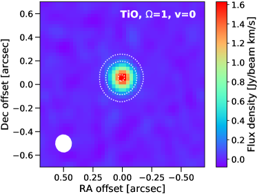
Figure 5: Zeroth moment map of the lowest fine structure component ($X^{3}\Delta_{1}$) of TiO in the ground ($v=0$) vibrational state observed in R Dor with ALMA. Indicated in white in the lower left corner is the $136\times 147$ mas beam. The white dotted contours indicate the continuum flux at levels of 1, 10, and 90% of peak flux.

Figure 6: Vibrational temperature diagram for TiO in R Dor derived from the $J=11-10$ rotational transition in the three spin components in the ground vibrational state and first excited $v=1$ vibrational level. Only two rotational transitions were observed in the $v=2$ level, because of the coincidence of the transition in the ${}^{3}\Delta_{2}$ component with a line of ³⁴SO₂.

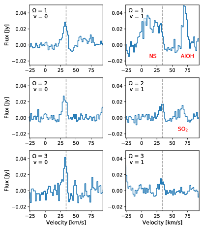
Figure 7: The $J=11\to 10$ rotational transition of TiO in the three fine structure components in the ground ($v=0$) and first excited vibrational level ($v=1$) observed towards IK Tau. The spectra were extracted from the ALMA data with an aperture whose radius is 160 mas. The grey dashed vertical lines indicate the expected center of the TiO line profiles for the assumed $\upsilon_{\mathrm{LSR}}=34$ km s^-1. Lines of other molecules are indicated in red.

For IK Tau the peak flux densities of the lines of TiO in the ground vibrational state are about 10 times lower than for R Dor (see Figures 7 and 11, and Table 4). Lines in the $v=1$ level in the $\Omega=2$ and $\Omega=3$ spin components were observed with a peak flux that is only two times higher than the rms noise, and no lines were detected in the $v=2$ level of TiO towards IK Tau. The $\Omega=1$ component of the line in the $v=1$ state is also undetected, due to a strong overlap with the NS line group at 346.22 GHz. The TiO emission from IK Tau is slightly blue-shifted with respect to the LSR velocity. Considering only the five detected lines shown in Fig. 7, we find a mean central velocity of $\upsilon_{\mathrm{cent(TiO)}}=32.4\pm 0.4$ km s^-1. This is offset from the $\upsilon_{\mathrm{LSR}}=34\pm 1$ km s^-1 of IK Tau (Decin et al., 2018) by 1.6 km s^-1 towards the blue, and could also be due to as-yet unknown inner wind dynamics. However owing to the estimated uncertainties in the rest frequencies and the low signal-to-noise of the data, confirmation of the apparent offset in velocity will require more accurate laboratory and more sensitive astronomical measurements.

4 Radiative Transfer Analysis of R Dor

4.1 Method

Due to the quality and availability of observations, we only performed radiative transfer analyses for R Dor. For this, we used a 1D spherically symmetric non-LTE radiative transfer program based on the accelerated lambda iteration method (ALI; Rybicki & Hummer, 1991; Maercker et al., 2008) to calculate the abundances and line profiles of AlO and TiO. The calculated line profiles were then compared with the lines of AlO or TiO observed with ALMA as described in Sects. 3.2.1 and 3.2.2.

For modelling purposes, we analyzed spectra extracted with a circular aperture with a radius of 150 mas, for AlO, and 300 mas, for TiO, because this included all the observed emission (see Sect. 3.2 for details). When ray-tracing our modelled CSE, we used (circular) model beams the same size as the extraction aperture, to allow for direct comparisons. Our model circumstellar envelopes (CSEs) were divided into 30 shells, evenly spaced on a logarithmic scale from an inner radius $r_{0}=3.3\times 10^{13}$ cm, out to an outer radius $r_{\mathrm{max}}=4\times 10^{14}$ cm. The velocity resolution of the model lines is approximately 0.5 km s^-1, however the final resolution of the AlO lines, taking hyperfine structure into account, is approximately 1 km s^-1, to match the resolution of the observations. The observed AlO lines are significantly broadened by the unresolved fine and hyperfine structure, and the TiO lines are split into three fine structure components as discussed in Sects. 2.1 and 2.2, respectively. In the following two sections (4.1.1 and 4.1.2) we describe our treatment of hyperfine structure for AlO and fine structure for TiO, respectively.

4.1.1 AlO

Explicitly including all the AlO hyperfine levels and the connecting transitions in the radiative transfer analysis is computationally prohibitive, even if the included levels are restricted to a relatively small number of rotational levels (e.g., $N\leq 20$). Following the procedure in Decin et al. (2017), AlO was first treated without hyperfine structure to obtain the total integrated line strengths for each observed transition. The calculated total integrated flux for each transition was then distributed among the individual hyperfine components according to their quantum mechanical line strengths (see Yamada et al., 1990; Goto et al., 1994; Launila & Jonsson, 1994; Launila & Banerjee, 2009). These were then summed to obtain the theoretical line profile shape. We used Gaussians with a HWHM of 3 km s^-1, close to the innermost velocity as derived from the sound speed, to represent the hyperfine components. In Sect. A.4 we discuss the impact of the choice of widths for the hyperfine components.

4.1.2 TiO

To analyze TiO in the most efficient way possible, we first ran a radiative transfer model excluding the fine structure — i.e., TiO was treated as though it were a closed shell molecule. To facilitate this, we took the energy levels and Einstein A coefficients from McKemmish et al. (2019) for the lowest fine structure component $\Omega=1$ (see the left hand panel of Fig. 1 for an overview of the fine structure in TiO). After running a radiative transfer model excluding the fine structure, we scaled the amplitude of the calculated line profiles to the relative intensities of the transitions in the three fine structure components tabulated in CDMS, on the assumption of LTE and a gas kinetic temperature of 1800 K, and compared our calculated profiles with the observed spectra. For $v>0$ we assumed the same intensity scaling for the fine structure components as those in the ground vibrational state (see Sect. 4.4).

4.2 Input parameters

4.2.1 Molecular parameters

A proper non-LTE analysis of the observations of the two metal oxides AlO and TiO requires the following molecular data: (1) Einstein $A$ coefficients for rotational transitions in the $v=0$ state; (2) Einstein $A$ coefficients for rotational transitions in the lower excited vibrational levels; (3) Einstein $A$ coefficients for the rovibrational $\Delta v=1,2,\cdots$ transitions; and (4) collisional rates for H₂–AlO and H₂–TiO. The Einstein $A$ coefficients for AlO and TiO were from Patrascu et al. (2015) and McKemmish et al. (2019), respectively. The collision rates for H₂–AlO and H₂–TiO have not been calculated. Instead the rates for He-SiO (Dayou & Balança, 2006) and He–NaCl (Quintana-Lacaci et al., 2016) — appropriately scaled to account for the difference in mass of these systems (see Schöier et al., 2005, for details) — were used as surrogates.

4.2.2 Stellar and circumstellar parameters

The circumstellar model in our radiative transfer calculations of AlO and TiO is based on the circumstellar models of R Dor presented in Maercker et al. (2016), Van de Sande et al. (2018), and Decin et al. (2017). The present model includes more observations of AlO and a larger number of energy levels and transitions than the one in Decin et al. (2017). The TiO model is based on the same circumstellar parameters as AlO, which are given in Table 5. This leaves $f_{\mathrm{molecule}}$, the inner molecular abundance (relative to H₂), as the only free parameter in our models.

Table 5: Stellar and circumstellar parameters for R Dor.

Property	Units		R Dor
$R_{\star}$	cm		$3.3\times 10^{13}$
$T_{\mathrm{eff}}$	K		2400
$D$	pc		59
$L_{\star}$	L⊙		6500
$\dot{M}$	$10^{-7}M_{\sun}$ yr-1		$1.6$
$\upsilon_{\infty}$	km $s^{-1}$		5.7
$\upsilon_{0}$	km $s^{-1}$		3
$\upsilon_{\rm{LSR}}$	km $s^{-1}$		7.0
$\upsilon_{\rm{turb}}$	km $s^{-1}$		1
$\epsilon$	$\cdots$		0.65
$\beta$	$\cdots$		1.5
$r_{0}$	cm		$3.3\times 10^{13}$
$r_{e}$	cm		$1\times 10^{14}$

The gas kinetic temperature was assumed to follow a power law radial profile (Decin et al., 2006, and references therein)

$$T_{\rm{gas}}(r)=T_{\mathrm{eff}}\left(\frac{R_{\star}}{r}\right)^{\epsilon},$$ (1)

with $\epsilon=0.65$, $T_{\mathrm{eff}}=2400$ K, and $R_{\star}=3.3\times 10^{13}$ cm. This value of $R_{\star}$ is derived from the implemented values of $T_{\mathrm{eff}}$ and $L_{\star}$, and is slightly larger than the value found by Norris et al. (2012) of $2.4\times 10^{13}$ cm (based on our implemented distance of 59 pc) or that used by Van de Sande et al. (2018) of $2.5\times 10^{13}$ cm, who also used a lower luminosity than ours of $4500~{}L_{\sun}$, whereas our luminosity value of $6500~{}L_{\sun}$ is that found by Maercker et al. (2016).

The parameterized $\beta$-type accelerating wind is described by

$$\upsilon_{\rm{gas}}(r)=\upsilon_{0}+(\upsilon_{\infty}-\upsilon_{0})\left(1-\frac{r_{0}}{r}\right)^{\beta},$$ (2)

where the inner wind velocity $\upsilon_{0}=3$ km s^-1 is set to the approximate sound speed, $\upsilon_{\infty}=5.7$ km s^-1 is the terminal expansion velocity, $r_{0}=R_{\star}$ is the radius at which the wind is launched, and $\beta=1.5$. The values of $\upsilon_{\infty}$ and $\beta$ were derived from an analysis of CO in R Dor by Maercker et al. (2016). We also include a constant turbulent velocity of $\upsilon_{\mathrm{turb}}=1$ km s^-1. The fractional abundance of AlO and TiO were represented by a Gaussian profile

$$f(r)=f_{\mathrm{molecule}}\exp\left(-\left(\frac{r}{r_{e}}\right)^{2}\right)~{},$$ (3)

centered on the central star, where $f_{\mathrm{molecule}}$ is the central abundance and $r_{e}$ is the $e$-folding radius. For both molecules, an $e$-folding radius of $1\times 10^{14}$ cm was used. For AlO this is the $e$-folding radius found by Decin et al. (2017). For TiO we don’t have any more detailed spatial information, since the emission is unresolved, but we assume a relatively compact distribution that we expect to be approximately similar to that of AlO.

4.3 AlO results

The AlO model presented in Decin et al. (2017) was specifically fit to the $N=9\to 8$ line in the ground vibrational state. Using the same model for the newer lines, we found that the $v=0$ lines were reasonably well reproduced, but it was not possible to reproduce the $v=2$ line since the Decin et al. (2017) model only included the ground vibrational state. When choosing how many vibrationally excited levels needed to be included in our model, we considered the effect of infrared pumping on the population of the rotational levels of AlO. Infrared emission of the central star has a maximum at around $1-2~{}\mu$m (Van de Sande et al., 2018), which is close to the term energies of the excited vibrational levels of AlO between $v=5$ and 10. Hence, we included all levels with $N<20$ and $v\leq 10$ as tabulated in ExoMol (Patrascu et al., 2015; Tennyson et al., 2016). Extending the molecular data in this way resulted in a well-reproduced $v=2$ line, while still giving well-reproduced $v=0$ lines.

Our best fitting model with the expanded molecular data described above has $f_{\mathrm{AlO}}=1.7\times 10^{-7}$ when using collisional rates based on the Dayou & Balança (2006) SiO rates (see Sect. A.1 for a more detailed discussion of collisional rates). Our modelled lines are plotted on the observed AlO lines in Fig. 8. As an aide for future observations, we have plotted in Fig. 9 the calculated line profiles for the $N=9-8$ transition in the $v=1$ and 3 excited vibrational levels derived from the same model. This shows the stark difference in width between transitions in different vibrational states.

The peak abundance we obtained is approximately 3% of the solar abundance of Al (Asplund et al., 2009). This is larger than that found by Decin et al. (2017) by a factor of two. This is most significantly due to the inclusion of the larger molecular dataset, since more levels are available to be populated and infrared pumping is able to contribute. The new observations of lines in the ground vibrational state provided some additional constraints on the model, but the identification of the $v=2$ line was also crucial for checking the completeness and accuracy of our model. In addition to the molecular data, we also needed to use a smaller inner radius of $R_{\star}$, compared with the $\sim 2R_{\star}$ value used by Decin et al. (2017), to properly reproduce the $v=2$ line.

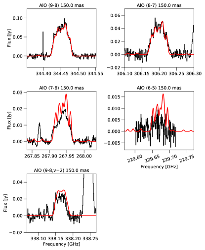
Figure 8: Spectra (black histograms) of rotational transitions of AlO observed towards R Dor, plotted with our synthetic profiles (red curves). Rotational (and vibrational for $v\neq 0$) quantum numbers and extraction aperture radii are indicated at the top of each box. The narrow feature at 267.871 GHz is the $15_{3,13}-15_{2,14}$ transition of ³⁴SO₂, and the intense line at 338.245 GHz is the $8-7,v=2$ transition of ²⁹SiO.

Figure 9: Synthetic line profiles of the $N=9-8$ rotational transition of AlO in the $v=1$ and $v=3$ excited vibrational states.

Although the model discussed above reproduces our AlO observations well, we investigated the effects of other factors which might possibly alter our results. In Sect. A.1 we discuss the effects of different choices of collisional rates. Ultimately, we found that the choice of collisional rates had a small but generally insignificant impact on our model results. In Sect. A.2, we discuss the impact of the choice of spectral extraction aperture on the final model results. In Sect. A.3 we test the influence of a disk on our model, such as that found by Homan et al. (2018). We found that including an approximation of a disk had some effect on our final results. We also tested the impact of an increased infrared radiation field on our results. This is discussed in detail at the end of Sect. 4.4 for TiO. We found that AlO is not very sensitive to increases in the infrared radiation field.

4.4 TiO results

Analogous with our radiative transfer analysis of AlO, we assumed that TiO could be described by a Gaussian distribution centered on the star with the same stellar and circumstellar parameters as in AlO, including the same $e$-folding radius $r_{e}=1\times 10^{14}$ cm (see Section 4.2.2 and Table 5). When adjusting our model to best reproduce the observations, we did not allow the fractional abundance of TiO to exceed the solar abundance of Ti (${\rm{Ti/H_{2}}}=1.8\times 10^{-7}$; Asplund et al., 2009). The initial analysis included rotational levels with $J\leq 20$ and vibrational levels with $v\leq 5$, and the velocity profile given by Eq. 2. The collisional rates for TiO were derived from the NaCl-He rates for a gas temperature of 700 K (Quintana-Lacaci et al., 2016), scaled for the difference in mass of the TiO-H₂ system (Schöier et al., 2005).

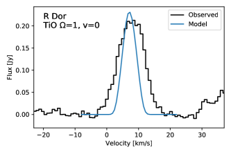
Figure 10: The $J=11-10$ rotational transition in the ${}^{3}\Delta_{1}$ spin component of TiO in the ground ($v=0$) vibrational state at 348,159.8 MHz observed towards R Dor (black histograms). A theoretical line profile calculated assuming a $\beta$-velocity law is shown in blue (see text for details).

From our first models, it was immediately apparent that the observed TiO lines are much broader than the line widths resulting from the velocity profile given in Eq. 2. A sample line from such a model with $f_{\mathrm{TiO}}=1.8\times 10^{-7}$ is shown in Fig. 10 and the full set of modelled and observed lines is shown in Fig. 16. Although the peak of the $v=0$ model line corresponds well with the observed peak, the calculated lines are $\sim 50\%$ of the observed $v=1$ peaks and less than $\sim 20\%$ of the $v=2$ peaks. We were able to better reproduce the widths of the observed lines by implementing a constant expansion velocity of 6 km s^-1 in place of the $\beta$-velocity law. However, in this case the peaks of the model lines significantly under-predicted the observations with the $v=0$ model lines at $\sim 40\%$ of the observed peaks and the $v>0$ model lines at $\lesssim 10\%$. Although it did not have a significant effect on our AlO model, we tested the effect of the “overdensity” model from Danilovich et al. (2020), with an increase in H₂ number density between $\sim 3R_{\star}$ and $4R_{\star}$ by a factor of 8. This model, with $f_{\mathrm{TiO}}=1.0\times 10^{-7}$, produced similar line peaks as the initial velocity law model, including under-predicting the higher-$v$ lines.

For AlO, our modelling could reproduce $v=0$ line when we included a larger number of vibrational states in our model. However, the vibrational levels included in the TiO input molecular data for $v\leq 5$ cover a similar extent in energy as those in AlO for $v\leq 10$, so we did not expect a significant difference when extending the included levels. Indeed, a test with TiO vibrational levels up to $v\leq 10$ confirmed this. Aside from vibrationally excited levels, TiO has many low-lying electronically excited states, for which McKemmish et al. (2019) provides line lists. The two lowest-lying electronic states are the singlet states $a\,^{1}\Delta$ and $d\,^{1}\Sigma^{+}$ whose term energies of $3~{}\mu$m and $1.8~{}\mu$m are close to the peak flux of the central star, and are also close to the term energies of the $v=3$ and $v=5$ excited vibrational levels of the ground electronic state (X$\,{}^{3}\Delta$). We tested models including these two singlet states, and including a larger complement of excited (singlet and triplet) states: $X\,^{3}\Delta$, $a^{1}\Delta$, $d^{1}\Sigma^{+}$, $b\,^{1}\Pi$, $E\,^{3}\Pi$, $A\,^{3}\Phi$, $B\,^{3}\Pi$, $C\,^{3}\Delta$, and $D\,^{3}\Sigma^{-}$. We found that including more electronic levels only caused incremental differences and small improvements in the model, and the model did not adequately reproduce the vibrationally excited lines. For clarity, we have included all the discussed models in Table 6.

Table 6: Parameters in the radiative transfer calculations of TiO in R Dor.

Model designation		Electronic states	Details
I.	$\beta$-velocity law	$X\,^{3}\Delta$	Parameters from Table 5, $f_{\mathrm{TiO}}=1.8\times 10^{-7}$, gas velocity from
			Eq. 2, rotational levels $J\leq 20$, and vibrational levels $v\leq 5$.
II.	$\upsilon_{\mathrm{gas}}=6$ km/s	$X\,^{3}\Delta$	As in I, but with a constant outward gas velocity $\upsilon_{\mathrm{gas}}=6$ km s-1
III.	Overdensity	$X\,^{3}\Delta$	As in II, but with the H2 number density 8 times higher for
			$\sim 3$–$4\,R_{\star}$ and $f_{\mathrm{TiO}}=1.0\times 10^{-7}$.
IV.	Singlet states	$X\,^{3}\Delta$, $a^{1}\Delta$, $d^{1}\Sigma^{+}$	As in III.
V.	Many excited states	$X\,^{3}\Delta$, $a^{1}\Delta$, $d^{1}\Sigma^{+}$, $b\,^{1}\Pi$, $E\,^{3}\Pi$,	As in III.
		$A\,^{3}\Phi$, $B\,^{3}\Pi$, $C\,^{3}\Delta$, $D\,^{3}\Sigma^{-}$
VI.	Higher IR field	$X\,^{3}\Delta$	As in III, but with an additional IR field.
VII.	Final model	$X\,^{3}\Delta$	As in VI, but with $f_{\mathrm{TiO}}=1.4\times 10^{-7}$.

All the models discussed until now have not taken dust into account since a significant fraction of the TiO (and AlO) emission comes from within the dust condensation radius found by Maercker et al. (2016). Including silicate dust with their derived opacity (optical depth of 0.05 at 10µm, Maercker et al., 2016) did not have a noticeable effect on the TiO (or AlO) emission. However, there is evidence of a gravitationally bound dust shell (Khouri, 2014) or ring (Khouri et al., 2016) in the innermost regions around R Dor, which may overlap with (or be the same object as) the rotating disc seen in molecular lines (Homan et al., 2018). Since the dust has been detected with infrared observations, we assume it contributes an additional infrared flux in the region of interest. To approximate this effect, we included an additional infrared radiation field in our model, based on a black body with a temperature of 1200 K. Although we have mainly discussed dust as the source of this additional infrared flux, there are other potential sources. In particular, the disc found by Homan et al. (2018) could be caused by a stellar or sub-stellar companion, such as a brown dwarf, which could also be a source of additional infrared flux. Another possible source is stellar fluctuations due to pulsations of the AGB star itself, especially if the stellar parameters used are biased towards fainter phases or epochs. To avoid the problems inherent in choosing just one of these scenarios, we approximate the presence of additional infrared flux using a uniform radiation field which does not vary with distance from the star. This is done using a source function derived from a black body with a temperature of 1200 K. This allows us to check the impact of an increased infrared flux, while leaving a more specific examination of the source of such flux to future work, since it is beyond the scope of this present study. With the inclusion of this additional infrared flux, we were finally able to reproduce all the TiO lines, including those in higher vibrational states. Our best fit model, which has $f_{\mathrm{TiO}}=1.4\times 10^{-7}$ is shown in Fig. 11, plotted with the observed spectra. Note that this model includes levels with $J\leq 20$, $v\leq 5$ and in the ground electronic state ($X\,^{3}\Delta$) only. The other models we tested, as detailed in entries I–VI in Table 6 are plotted in Fig. 16 in the appendix.

For completion, we tested a model including the increased infrared radiation field for AlO and found no significant difference between that model and the best model found in Sect. 4.3. This is most likely due to the significant difference in Einstein A coefficients for vibrational transitions, which are approximately 30 times larger for TiO than AlO when considering the rotational levels of interest here. This implies that the radiative lifetimes of the excited vibrational levels are shorter for TiO than for AlO, hence a higher infrared flux is needed to maintain sufficient population of vibrationally excited TiO molecules in the higher vibrational levels, to compensate for the shorter lifetimes. Conversely, the longer radiative lifetimes for AlO mean that an increased infrared flux is not needed to maintain the population of vibrationally excited AlO molecules, and hence does not result in a significantly higher amount of radiative pumping.

Figure 11: The $J=11\to 10$ rotational transitions of TiO observed towards R Dor (black histograms) with the vibrational levels ($v$) and fine structure components ($\Omega$) noted in the top left corner of each plot. Model profiles are overplotted in red and the vertical dashed grey lines indicate the LSR velocity of 7 km s^-1. Nearby lines are labelled with blue text.

5 Discussion and conclusions

5.1 Our results in context

Our radiative transfer calculations confirm the importance of infrared radiative pumping on the excitation of AlO and TiO in the inner wind of R Dor when observed at high angular resolution. For AlO, we found the most important factor was including sufficient vibrationally excited levels to facilitate infrared pumping. However for TiO, we needed to include a sufficiently high infrared flux to reproduce lines in the higher vibrational levels (with $v>0$). Such a flux, however, did not have an effect on our AlO results.

It is apparent from this and prior work on AlO and TiO in R Dor (see Sects. 3.2 and 4) that a substantial fraction of both molecules are located in a region close to the central star — i.e., $\sim$50% of gaseous AlO is within the dust condensation radius, and likely a larger fraction of TiO since we only have spatially unresolved observations. A direct determination of the size of the compact molecular emission is limited by the angular resolution in the present observations ($\sim$140 mas, or 2.5 times the stellar diameter $\theta_{\rm{d}}$; Decin et al., 2018). As a result, we can only determine the compact molecular emission is from a region within $\sim$70 mas or $\sim 2\,R_{\star}$ of the central star ($R_{\star}\simeq 30$ mas Norris et al., 2012). However, the radiative transfer analysis of the line profiles has yielded some additional confirmation of the location of AlO and TiO near and within the dust condensation radius.

5.1.1 AlO

Our observations of four successive rotational transitions of AlO in the ground vibrational state and one in the second excited ($v=2$) vibrational level are well-reproduced with our radiative transfer model when we included an adequate number of vibrationally excited levels (up to $v\leq 10$, see Sect. 4.3). The model reproduces molecular emission which encompasses the region between the stellar photosphere and the region in which dust starts to condense and extends beyond the dust condensation radius (see Sect. 4; Decin et al., 2017; Danilovich et al., 2016, 2020, and references therein).

Our revised fractional abundance of AlO in R Dor ($f_{0}=1.7\times 10^{-7}$) is about 2 times higher than the earlier estimate by Decin et al. ($8.4\times 10^{-8}$, 2017), but it is still much lower than the solar abundance of Al ($5.6\times 10^{-6}$, with respect to H₂; Asplund et al., 2009). Hence, this result does not preclude the possibility of AlO being incorporated into dust, even in regions overlapping with our model region.

5.1.2 TiO

The line profiles of TiO are wider than expected based on the assumption of the velocity law given in Eq. 2, derived from older (less sensitive) single-antenna observations of R Dor (e.g Maercker et al., 2016, who find $\upsilon_{\infty}=5.7$ km s^-1). Lines wider than the previously determined expansion velocity have been seen for other molecules observed by ALMA. For example, there are faint wings either side of the intense emission lines of CO, SiO, and SO in the ground vibrational state (also observed in the ALMA spectral line survey of R Dor, Decin et al., 2018). A more detailed analysis of the SO emission by Danilovich et al. (2020) found that the SO lines in the first vibrationally excited state were wider than the HWHM of the $v=0$ lines; that is, rather than just faint wide wings, the $v=1$ lines were overall as wide as the wings of the $v=0$ lines. This was interpreted as emission coming from a rotating disk close to the central star, such as that reported by Homan et al. (2018), with a rotational velocity greater than the expansion velocity. In an LTE analysis of four rotational lines of OH in non-maser emission from high lying rotational lines in R Dor, Khouri et al. (2019) estimated the FWHM of the OH emission region is about $70\pm 20$ mas with possible evidence for line broadening. This is likely due to the same underlying physical phenomenon. The adjustments we made to our TiO model of a higher constant velocity and the inclusion of an overdense region support the rotating disk interpretation. Although the implemented expansion velocity of 6 km s^-1 is unphysical in a region so close to the star, it can be thought of here as a partial 1D approximation of the rotating disk.

The presence of photospheric TiO in M-type stars, as seen in bands in the optical and infrared regimes, has long been known and have been used in the spectral classification of these stars (see for example Gray et al., 2009, and references therein). Hence, it is not unexpected that we also detect rotational transitions of TiO close to the surface of the star. However, since our observations are not spatially resolved, we are unable to properly constrain the extent of the TiO emission, other than it is within $\sim 75$ mas of the star, based on the ALMA beam size of $\sim 150$ mas.

Our derived abundance of TiO is $1.4\times 10^{-7}$ relative to H₂, which is close to the solar abundance of Ti ($1.8\times 10^{-7}$ Asplund et al., 2009). This does not leave much Ti for the possible formation of TiO₂ if we assume that TiO₂ is present in the same region as TiO. Evidence for the presence of TiO₂ is discussed in the following Section 5.2. Since the TiO we detect is close to the star and mostly or entirely within the dust condensation radius, our results do not preclude the incorporation of TiO into dust grains. In fact, a role in dust formation or growth would explain the lack of TiO detections further from the star. It is possible that our apparent high abundance of TiO may rather be attributable to the complex density and velocity structures before the wind acceleration zone in R Dor, as revealed in recent polarimetric observations in the optical and near infrared at high angular resolution (Khouri et al., 2016) and predicted in theoretical dust driven models (Höfner et al., 2016, and references therein).

5.2 Evidence for gas-phase TiO₂ towards R Dor

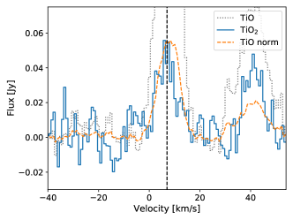
Figure 12: The TiO₂ ($26_{0,26}\to 25_{1,25}$) line at 350.399 GHz (blue histograms) plotted with the TiO $J=11\to 10$, $\Omega=1$ line in the ground vibrational state (grey dotted line). We also show the same TiO line scaled down to the same peak intensity as the TiO₂ line, to allow for a comparison of line profile shapes. The vertical black dashed line represents the systemic LSR velocity of 7 km s^-1 for R Dor.

In an earlier survey of R Dor using the APEX telescope, De Beck & Olofsson (2018) found some very tentative evidence for TiO₂ when stacking 18 lines covered by their frequency range. Using the more sensitive ALMA telescope, Decin et al. (2018) observed some possible TiO₂ lines as part of the previously discussed Band 7 spectral line survey of R Dor (observation ID 2013.1.00166.S). We examined the identified lines in more detail and determined that several lines are uncertain, in large part due to overlaps with other nearby lines. In discussing TiO₂ below, we primarily refer to the more certain identifications of lines that we do not believe participate in overlaps, and in particular the following three lines: ($26_{0,26}\to 25_{1,25}$) at 350.399 GHz, ($25_{2,24}\to 24_{1,23}$) at 350.708 GHz, and ($24_{2,22}\to 23_{3,21}$) at 347.788 GHz, listing in descending order of predicted intensity. We plot one of these lines, ($26_{0,26}\to 25_{1,25}$) at 350.399 GHz with the TiO $v=0$, $\Omega=1$ line in Fig. 12, showing the TiO line as observed and scaled down to the same peak flux as the TiO₂ line. The rotational lines of TiO₂ are 4–5 times less intense than those of TiO, and the line profile shape may be narrower. However, the low intensity and lower signal to noise ratio of the TiO₂ lines makes it difficult to conduct any conclusive analysis, since even the brightest lines, such as that shown in Fig. 12 are only just detected above the noise. The TiO₂ emission is also unresolved in our channel maps and zeroth moment maps, supporting the contention that it is located close to the star. This is feasible since gaseous TiO₂ is made by the temperature dependent exothermic reaction

$${\rm TiO}+{\rm OH}\rightarrow{\rm TiO_{2}}+{\rm H}\,,$$ (4)

which is very fast at the temperatures within a few stellar radii of oxygen rich AGB stars (see Fig. 2 in Plane, 2013).

An estimate of the column density of TiO₂, derived from a single transition in the ground vibrational state ($26_{0,26}\to 25_{1,25}$) at 350.399 GHz) on the assumption that the excitation temperature is 1800 K, was comparable to the column density of TiO found in our models. However, this value is very uncertain and does not conclusively imply that there is a similar abundance of TiO₂ as TiO (and hence we do not suggest that there is a higher abundance of Ti in R Dor than in the Sun).

Other related laboratory work concerns the low abundance of TiO₂ in the few presolar grains that have been analyzed (Stroud et al., 2004; Nittler et al., 2008). However, owing to the limitation of available samples, the sophisticated laboratory instruments used to analyze the presolar grains from low mass AGB stars might not be sensitive enough to detect TiO₂ seed crystals if they were very small (L. Nittler, personal communication).

It has also been noted the abundance of TiO and TiO₂ derived from the rotational spectra in at least one source (Mira A, see Kamiński et al., 2017, and discussion in Sect 1) appears too low to account for the total mass of the dust in the dust forming region if the dust were composed of TiO₂. Yet there is substantial depletion of Ti in the interstellar medium by about 0.1 or higher (Jenkins, 2009), suggesting TiO₂ might be involved in dust formation. And as Boulangier et al. (2019) showed, the number of TiO₂ clusters formed in their chemical code ($n({\rm{TiO}}_{2})_{1000}/n_{H}\sim 10^{-11}$) should be sufficient to drive a wind and still be left with a large abundance of gaseous TiO₂/TiO/Ti.

Unfortunately, rotational lines of vibrationally excited TiO₂ have not been observed in the laboratory, nor in oxygen-rich AGB or RSG stars (for a more comprehensive look at TiO₂ in VY CMa, see Kamiński et al., 2013b). This leaves us with few comparisons and little room to draw any definite conclusions regarding TiO₂.

5.3 Dust precursors and dust formation

Optical and infrared observations of R Dor and W Hya, another oxygen-rich AGB star with a low mass-loss rate, established that there are transparent dust grains within $\lesssim 2R_{\star}$ of the central star (Norris et al., 2012; Khouri et al., 2016; Ohnaka et al., 2016). The composition of the dust grains has not been conclusively confirmed, but the present evidence points to alumina (Al₂O₃) as the probable carrier of spectral features in the mid IR, as observed at low angular resolution with ISO SWS (see Khouri, 2014; Decin et al., 2017, and references therein). More recently, these and other oxygen-rich AGB stars have been observed at much higher angular resolution using mid and near IR interferometry (Karovicova et al., 2013; Ohnaka et al., 2016), polarimetric interferometry (Norris et al., 2012), and polarimetric imaging (Khouri et al., 2016; Ohnaka et al., 2016).

There has been a long standing debate about the formation mechanism(s) of solid Al₂O₃ grains from gas phase species, and whether it entails a homogenous or a heterogenous process. Gail & Sedlmayr (1998, 1999) concluded — on the assumption of chemical equilibrium in the gas phase, approximate nucleation theories, and extrapolation of bulk properties to gas phase clusters — that a heteromolecular process in which small aluminum bearing oxides and hydroxides (e.g., AlOH, Al₂O, and Al₂O₂) condense on a grain surface and subsequently react to produce the Al₂O₃ grains appears most probable. This is because the abundance of gaseous Al₂O₃ is predicted to be far too low to form solid Al₂O₃ by homogenous nucleation of gaseous Al₂O₃ and subsequent condensation on TiO₂ nucleation seeds (Jeong et al., 2003).

There have also been some important advances in supporting laboratory measurements in the past 20 years. These include measurements of the IR-REMPI spectra of large gas phase (Al₂O₃)_n and (TiO₂)_n clusters which provide accurate wavelengths of the vibrational bands in the IR, and establish Al₂O₃ and TiO₂ clusters can form in the gas phase under the specific conditions in the laboratory (Demyk et al., 2004), but it is uncertain whether the same conditions apply within a couple of stellar radii of the low mass oxygen rich AGB stars.

In a recent study, Boulangier et al. (2019) examined four precursor candidates of the dust with their self-consistent wind model of oxygen rich AGB stars: TiO₂, MgO, SiO, and Al₂O₃. On the basis of theoretical quantum chemical calculations, they found there is a sharp threshold in temperature of 1000–1200 K when (TiO₂)₁₀ clusters form in their model AGB star; the abundance of the (TiO₂)_n clusters is orders of magnitude lower at temperatures greater than 1200 K; Al₂O₃ clusters are predicted at temperatures as high as 1800–2400 K; and nearly all the available Al₂O₃ monomers are tied up in the clusters at slightly lower temperatures of $1600-2200$ K. Boulangier et al. (2019) ruled out TiO₂ clusters as nucleation seeds, because the observations establish the dust exists close to the central star where the temperatures are as high as $1500-2000$ K. However the uncertainties in the quantum calculations of the temperature ranges are difficult to quantify. Also as they note, their “comprehensive” chemical kinetic code, which starts with atomic constituents, has several significant shortcomings: it includes a relatively modest chemical network ($\sim 330$ reactions) and, although TiO₂ and its clusters are produced, their kinetic code does not form the Al₂O₃ monomer or its clusters; AlO₂ and Al₂O₂ — the suspected precursors of Al₂O₃ — are not produced; and Mg remains in the atomic form and does not form MgO.

In view of the current understanding of dust formation, further astronomical observations, and accompanying radiative transfer analysis of the suspected gas phase precursors in the ground and excited vibrational levels at high angular resolution and sensitivity are needed in conjunction with: polarimetric observations in the optical and near IR, theoretical calculations, supporting laboratory measured reaction rates and product distributions, and laboratory measurements of the rotational spectra of key species in the kinetic models. At present the relevant astronomical observations are available for just a couple of specific sources, and there is insufficient information to determine whether what we see are general trends in these types of sources. For example, it is unclear whether gravitationally bound dust shells are prevalent in oxygen rich AGB stars with low mass loss rates as suspected (Höfner & Olofsson, 2018), or whether the Al₂O₃ dust (and by inference gaseous AlO) and gravitationally bound dust shells are intimately connected in these objects, or whether TiO₂ are the seeds of the alumina dust.

Appendix A Further detailed investigation of AlO modelling

A.1 Choice of collisional rates for AlO

Since the cross sections for collisions between AlO and H₂ have not been measured or calculated, we tested the dependence of our radiative transfer model on the choice of collisional rates. We implemented collisional rates calculated for two other molecular systems: (1) SiO colliding with He which only includes levels in the ground vibrational state (Dayou & Balança, 2006); and (2) NaCl with He which includes rotational levels in the ground and vibrationally excited states, and ro-vibrational collisional transitions (Quintana-Lacaci et al., 2016). In both systems, the collisional rates were scaled for the difference in mass with that of AlO–H₂ (Schöier et al., 2005).

To test the influence of the collisional excitation rates on the solutions to the statistical equations in the radiative transfer analysis, we also ran models with (3) the collision rates adapted from the NaCl rates multiplied by 100, and (4) all the collision rates set to zero. To compare the dependence of the models on the different collisional rates, we first determined the best fitting model with the collisional rates adapted from the SiO rates ($f_{\mathrm{AlO}}=1.7\times 10^{-7}$), and then used the same AlO abundance profile to run models with the other sets of collisional rates. Plotted in Fig. 13 are all the calculated line profiles superposed on the observed spectra.

The difference between the calculated lines profiles and the observed lines for the different sets of collisional rates was negligible in the ground vibrational state and was small for the line in the excited $v=2$ level. The most significant departure was for the model with the collisions adapted from NaCl multiplied by 100, which resulted in only a minor difference for the $v=0$ lines, but produced a profile for the $v=2$ line that was 30% less intense than the corresponding line calculated for NaCl collisions cross sections that were not multiplied by 100. The model which neglected collisional excitation predicted slightly brighter lines for all observed transitions than the models for which collisions were considered.

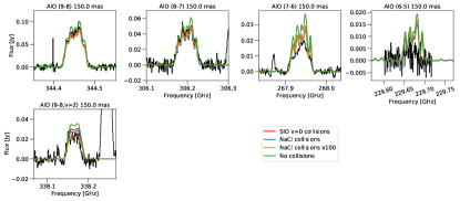
Figure 13: Spectra (black histograms) of four successive rotational transitions of AlO in the ground vibrational state and one transition in the second excited ($v=2$) level observed towards R Dor; and synthetic profiles (coloured curves). Rotational quantum numbers and the extraction aperture radii are indicated at the top of each box.

A.2 Impact of the south-eastern extension in AlO emission

When selecting spectra to use to constrain our 1D radiative transfer models of R Dor, we selected AlO spectra extracted for a 150 mas radius aperture. This is in contrast with the 300 mas aperture spectra selected for TiO, which were chosen to capture the maximum amount of TiO flux, without being dominated by noise. In the case of AlO, a smaller aperture was selected to avoid including the SE extension seen in the zeroth moment maps of Fig 3. The extension breaks spherical symmetry and hence cannot be reproduced by a 1D model.

To emphasise the impact the SE extension and our choice of aperture, we plot in Fig. 14 the same model as shown in Fig. 8 but for a spectral extraction aperture of 300 mas. The differences between Figures 8 and 14 clearly show the impact of the SE extension: the ground state lines of ($9\to 8$) and ($8\to 7$) are slightly under-predicted when additional emission from the SE extension is included in the observed spectra; and the ($7\to 6$) and ($6\to 5$) lines are less over-predicted for the same reason. In addition, the 150 mas extraction of the ($6\to 5$) is strongly affected by resolved-out flux, which is a less prominent problem for the 300 mas aperture spectrum, since the latter is more strongly dominated by noise.

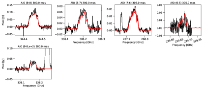
Figure 14: Spectra (black histograms) of four successive rotational transitions of AlO in the ground vibrational state and one transition in the second excited ($v=2$) level observed towards R Dor; and synthetic profiles (red curves) calculated with our best radiative transfer model. Data and models are shown for a spectral extraction aperture radius of $\sim 300$ mas.

A.3 The effects of a disk

In addition to investigating the impact of the particular set of collisional rates adopted, we checked the effect of a possible disk in the inner regions of R Dor (see Homan et al., 2018) on our radiative transfer analysis of AlO. Because our model is 1-dimensional and cannot fully reproduce a disk, we referred to the spherically symmetric approximations implemented by Danilovich et al. (2020) in their analysis of SO around the same star. Specifically, we tested the effect of their “overdensity” model in which the H₂ number density between $\sim 3R_{\star}$ and $4R_{\star}$ was increased by a factor of 8. Due to the overlap between this overdensity region and the region where AlO is primarily observed, the new model does result in brighter AlO line profiles. Using this overdensity model, we adjusted our AlO abundance until we were able to once again reproduce the observed lines. From this we found a new best fit model with $f_{\mathrm{AlO}}=7\times 10^{-8}$ relative to H₂. This is more than a factor of two lower than our original model that does not include an overdense region.

A.4 Widths of hyperfine components

In addition to the above, we tested the effect of the assumed widths of the theoretical Gaussian profiles representing the unresolved hyperfine components of the very broad AlO lines. In general, smaller assumed widths resulted in calculated line profiles in which the underlying hyperfine structure is more noticeable, while larger widths resulted in smoother line profile shapes. Although we present our final model with HWHM widths set to 3 km s^-1, we tested different HWHM widths for all the lines. We found the theoretical line profiles which yielded the best fits were 3 km s^-1 for the $N=9\to 8$ and $8\to 7$ lines, and 4.5 km s^-1 for the $7\to 6$ line. The $6\to 5$ line is omitted from this analysis due to lower data quality, but generally appears to correspond better with a larger HWHM. The tightest observational constraints were found for the $N=9\to 8$ and $7\to 6$ transitions in the ground vibrational state, where wider Gaussian components produced a smoother line profile than was observed for the $9\to 8$ line, and narrower components produced a jagged line profile that did not reproduce the $7\to 6$ line well. As shown in Fig. 15, the profile constructed from the 5.7 km s^-1 hyperfine components does not reproduce the hyperfine structure observed with ALMA for the $9\to 8$ line, whereas the the profile constructed from 3 km s^-1 hyperfine components (also shown in Fig. 8 for all lines) is more jagged than the observed $7\to 6$ profile.

The good agreement between most of the observed and synthetic line profiles for the 3 km s^-1 hyperfine components is part of the reason this value was chosen for the final model. However, we cannot easily explain why the $7\to 6$ line has smoother or less distinct hyperfine components. One possible explanation is that, as a lower-energy line, it is formed further out in the envelope. However, the zeroth moment map of the emission (see Fig. 3) and the emission extents predicted by our (spherically symmetric) radiative transfer model do not support this hypothesis. (Note that the apparent larger size of the emission shown in Fig. 3 is mainly due to differences in sensitivity between the $7\to 6$ and $8\to 7$ observations.) Our radiative transfer model cannot account for non-spherically symmetric features, so it is possible the $7\to 6$ line is excited more in (the faster rotating portion of) the disc than the other transitions. This is not something we can check with our current level of observations, however.

Figure 15: Synthetic line profiles for two transitions of AlO towards R Dor calculated using two different HWHM (3 km s^-1 and 5.7 km s^-1) for the Gaussians representing the hyperfine components. These curves are plotted over the observed line profiles, which are shown as green histograms.

Appendix B Further details of tested TiO models

In Fig. 16 we plot the TiO models discussed in Sect. 4.4 and tabulated in entries I–VI of Table 6. Our final TiO model, entry VII in Table 6, is not included here and can instead be seen in Fig. 11.

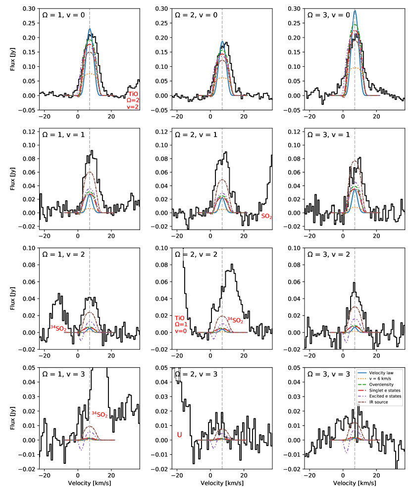
Figure 16: The $J=11-10$ rotational transitions of TiO observed towards R Dor (black histograms) with the vibrational levels ($v$) and fine structure components ($\Omega$) noted in the top left corner of each plot. Model profiles are overplotted in red and the vertical dashed grey lines indicate the LSR velocity of 7 km s^-1. Nearby lines are labelled with red text.

Appendix C Theoretical structures of small aluminum oxides

There has been some confusion in the astronomical literature regarding the structures of the most stable forms of the small aluminum oxides, owing to earlier calculations in the chemical literature at low levels of theory. Presented here are couple cluster theory calculations of three aluminum oxides frequently cited as possible precursors of Al₂O₃: Al₂O (Fig. 17), AlO₂ (Fig. 18), and Al₂O₂ (Fig. 19).

C.1 Al₂O

There are three possible arrangements of the nuclei in Al₂O (a $C_{2v}$ form like H₂O, a $D_{\infty h}$ form like CO₂, and a $C_{\infty v}$ form Al–Al–O), and two possible electron spin multiplicities (singlet and triplet). Summarized in Figure 17 are the calculated structures, permanent electric dipole moments, and relative energies at the ae-CCSD(T)/cc-pWCVTZ level of theory, where the zero-point energy was estimated with a smaller basis (cc-pWCVDZ).

The Al₂O isomers with triplet multiplicity are at least 33,000 K or higher in energy than the singlet structures. Singlet Al–O–Al is the most stable isomer and is probably the most abundant isomer in the inner wind of oxygen rich AGB stars, but it is nonpolar and the rotational spectrum is unobservable with radio telescopes. Two of the remaining three isomers possess large dipole moments and have structures with $C_{\infty v}$ symmetry — one is a singlet and the other is a triplet. The triplet $C_{2v}$ form is calculated to be the lowest energy polar form of Al₂O, although it might prove difficult to detect because it possesses a small dipole moment (0.8 D), and it is nearly degenerate (to within ${\sim}2500$ K) with the $D_{\infty h}$ structure. Depending on how well the relative energies are determined, the $D_{\infty h}$ structure might undergo thermal interconversion between the polar and nonpolar forms in the hot inner wind close to the central star, and therefore warrants a more sophisticated quantum chemical treatment.

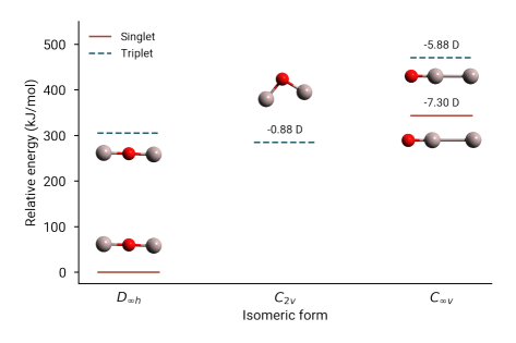
Figure 17: Relative energies and dipole moments of the isomers of Al₂O.

C.2 AlO₂

To assess whether the rotational spectrum of AlO₂ (all with doublet electron spin multiplicity) might be detectable with radio telescopes, we calculated the electronic and zero-point energy, and the dipole moments at the ae-CCSD(T)/cc-pWCVTZ level of theory (Figure 18). The most stable isomer is the nonpolar $D_{\infty h}$ structure, followed by the isomer with $C_{2v}$ symmetry, and a linear $C_{\infty v}$ isomer. The dipole moments of the polar isomers are modest, perhaps indicating their detection in the inner wind of oxygen rich AGB stars might be difficult. The calculated quadrupole coupling constant ($eQq$) of $-20.9$ MHz for the $C_{2v}$ isomer and $-26.6$ MHz for the $C_{\infty v}$ isomer are similar to that of AlO ($eQq=-26.1\pm 0.21$ MHz; Goto et al., 1994), implying the Al—O bonding character is very similar in AlO and AlO₂.

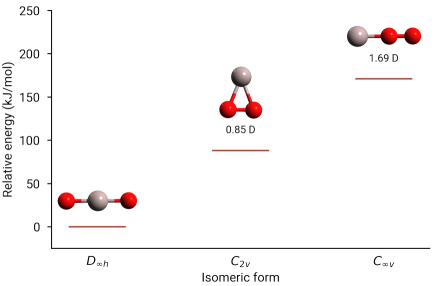
Figure 18: Relative energies and dipole moments of three isomers of AlO₂ with electron spin multiplicity of 2.

C.3 AlOAlO

Linear AlOAlO (see Fig. 19) is an attractive candidate for astronomical detection in oxygen rich stars. It has been observed at IR wavelengths trapped in an inert matrix (Andrews et al., 1992), and the permanent electric dipole moment is large (5.16 D; S. Thorwirth, personal communication). Owing to its rigid linear geometry, the rotational spectrum of AlOAlO consists of a single series of harmonically related rotational transitions spaced every 3.4 GHz apart.

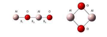
Figure 19: The two most stable isomers of Al₂O₂. The linear AlOAlO isomer is estimated to be 1,500 K higher in energy than the most stable (cyclic) isomer of Al₂O₂, but the rotational spectrum of the symmetric cyclic isomer is not observable.

References

- Andrews et al. (1992) Andrews, L., Burkholder, T. R., & Yustein, J. T. 1992, The Journal of Physical Chemistry, 96, 10182, doi: 10.1021/j100204a018
- Asplund et al. (2009) Asplund, M., Grevesse, N., Sauval, A. J., & Scott, P. 2009, ARA&A, 47, 481, doi: 10.1146/annurev.astro.46.060407.145222
- Boulangier et al. (2019) Boulangier, J., Gobrecht, D., Decin, L., de Koter, A., & Yates, J. 2019, MNRAS, 489, 4890, doi: 10.1093/mnras/stz2358
- Breier et al. (2019) Breier, A. A., Waßmuth, B., Fuchs, G. W., Gauss, J., & Giesen, T. F. 2019, Journal of Molecular Spectroscopy, 355, 46, doi: 10.1016/j.jms.2018.11.006
- Danilovich et al. (2016) Danilovich, T., De Beck, E., Black, J. H., Olofsson, H., & Justtanont, K. 2016, A&A, 588, A119, doi: 10.1051/0004-6361/201527943
- Danilovich et al. (2020) Danilovich, T., Richards, A. M. S., Decin, L., Van de Sande, M., & Gottlieb, C. A. 2020, MNRAS, 494, 1323, doi: 10.1093/mnras/staa693
- Dayou & Balança (2006) Dayou, F., & Balança, C. 2006, A&A, 459, 297, doi: 10.1051/0004-6361:20065718
- De Beck & Olofsson (2018) De Beck, E., & Olofsson, H. 2018, A&A, 615, A8, doi: 10.1051/0004-6361/201732470
- De Beck et al. (2015) De Beck, E., Vlemmings, W., Muller, S., et al. 2015, A&A, 580, A36, doi: 10.1051/0004-6361/201525990
- Decin et al. (2006) Decin, L., Hony, S., de Koter, A., et al. 2006, A&A, 456, 549, doi: 10.1051/0004-6361:20065230
- Decin et al. (2018) Decin, L., Richards, A. M. S., Danilovich, T., Homan, W., & Nuth, J. A. 2018, A&A, 615, A28, doi: 10.1051/0004-6361/201732216
- Decin et al. (2017) Decin, L., Richards, A. M. S., Waters, L. B. F. M., et al. 2017, A&A, 608, A55, doi: 10.1051/0004-6361/201730782
- Demyk et al. (2004) Demyk, K., van Heijnsbergen, D., von Helden, G., & Meijer, G. 2004, A&A, 420, 547, doi: 10.1051/0004-6361:20034117
- Gail & Sedlmayr (1998) Gail, H. P., & Sedlmayr, E. 1998, Faraday Discussions, 109, 303, doi: 10.1039/a709290c
- Gail & Sedlmayr (1999) —. 1999, A&A, 347, 594
- Gobrecht et al. (2016) Gobrecht, D., Cherchneff, I., Sarangi, A., Plane, J. M. C., & Bromley, S. T. 2016, A&A, 585, A6, doi: 10.1051/0004-6361/201425363
- González Delgado et al. (2003) González Delgado, D., Olofsson, H., Kerschbaum, F., et al. 2003, A&A, 411, 123, doi: 10.1051/0004-6361:20031068
- Goto et al. (1994) Goto, M., Takano, S., Yamamoto, S., Ito, H., & Saito, S. 1994, Chemical Physics Letters, 227, 287, doi: 10.1016/0009-2614(94)00820-5
- Gray et al. (2009) Gray, R., Corbally, C., & Burgasser, A. 2009, Stellar Spectral Classification, Princeton Series in Astrophysics (Princeton University Press)
- Höfner et al. (2016) Höfner, S., Bladh, S., Aringer, B., & Ahuja, R. 2016, A&A, 594, A108, doi: 10.1051/0004-6361/201628424
- Höfner & Olofsson (2018) Höfner, S., & Olofsson, H. 2018, A&A Rev., 26, 1, doi: 10.1007/s00159-017-0106-5
- Homan et al. (2018) Homan, W., Danilovich, T., Decin, L., et al. 2018, A&A, 614, A113, doi: 10.1051/0004-6361/201732246
- Ito & Goto (1994) Ito, H., & Goto, M. 1994, Chemical Physics Letters, 227, 293 , doi: https://doi.org/10.1016/0009-2614(94)00821-3
- Jenkins (2009) Jenkins, E. B. 2009, ApJ, 700, 1299, doi: 10.1088/0004-637X/700/2/1299
- Jeong et al. (2003) Jeong, K. S., Winters, J. M., Le Bertre, T., & Sedlmayr, E. 2003, A&A, 407, 191, doi: 10.1051/0004-6361:20030693
- Kamiński (2019) Kamiński, T. 2019, in IAU Symposium, Vol. 343, IAU Symposium, ed. F. Kerschbaum, M. Groenewegen, & H. Olofsson, 108–118, doi: 10.1017/S1743921318006038
- Kamiński et al. (2013a) Kamiński, T., Gottlieb, C. A., Young, K. H., Menten, K. M., & Patel, N. A. 2013a, ApJS, 209, 38, doi: 10.1088/0067-0049/209/2/38
- Kamiński et al. (2013b) Kamiński, T., Gottlieb, C. A., Menten, K. M., et al. 2013b, A&A, 551, A113, doi: 10.1051/0004-6361/201220290
- Kamiński et al. (2016) Kamiński, T., Wong, K. T., Schmidt, M. R., et al. 2016, A&A, 592, A42, doi: 10.1051/0004-6361/201628664
- Kamiński et al. (2017) Kamiński, T., Müller, H. S. P., Schmidt, M. R., et al. 2017, A&A, 599, A59, doi: 10.1051/0004-6361/201629838
- Karovicova et al. (2013) Karovicova, I., Wittkowski, M., Ohnaka, K., et al. 2013, A&A, 560, A75, doi: 10.1051/0004-6361/201322376
- Khouri (2014) Khouri, T. 2014, PhD thesis, Univeristy of Amsterdam
- Khouri et al. (2019) Khouri, T., Velilla-Prieto, L., De Beck, E., et al. 2019, A&A, 623, L1, doi: 10.1051/0004-6361/201935049
- Khouri et al. (2018) Khouri, T., Vlemmings, W. H. T., Olofsson, H., et al. 2018, A&A, 620, A75, doi: 10.1051/0004-6361/201833643
- Khouri et al. (2015) Khouri, T., Waters, L. B. F. M., de Koter, A., et al. 2015, A&A, 577, A114, doi: 10.1051/0004-6361/201425092
- Khouri et al. (2016) Khouri, T., Maercker, M., Waters, L. B. F. M., et al. 2016, A&A, 591, A70, doi: 10.1051/0004-6361/201628435
- Knapp et al. (2003) Knapp, G. R., Pourbaix, D., Platais, I., & Jorissen, A. 2003, A&A, 403, 993, doi: 10.1051/0004-6361:20030429
- Launila & Banerjee (2009) Launila, O., & Banerjee, D. P. K. 2009, A&A, 508, 1067, doi: 10.1051/0004-6361/200913274
- Launila & Berg (2011) Launila, O., & Berg, L. E. 2011, Journal of Molecular Spectroscopy, 265, 10, doi: 10.1016/j.jms.2010.10.005
- Launila & Jonsson (1994) Launila, O., & Jonsson, J. 1994, Journal of Molecular Spectroscopy, 168, 1, doi: 10.1006/jmsp.1994.1257
- Levesque (2017) Levesque, E. M. 2017, Astrophysics of Red Supergiants (IOP Publishing), doi: 10.1088/978-0-7503-1329-2
- Lovas & Tiemann (1974) Lovas, F. J., & Tiemann, E. 1974, Journal of Physical and Chemical Reference Data, 3, 609
- Maercker et al. (2016) Maercker, M., Danilovich, T., Olofsson, H., et al. 2016, A&A, 591, A44, doi: 10.1051/0004-6361/201628310
- Maercker et al. (2008) Maercker, M., Schöier, F. L., Olofsson, H., Bergman, P., & Ramstedt, S. 2008, A&A, 479, 779, doi: 10.1051/0004-6361:20078680
- McKemmish et al. (2019) McKemmish, L. K., Masseron, T., Hoeijmakers, H. J., et al. 2019, MNRAS, 488, 2836, doi: 10.1093/mnras/stz1818
- Namiki et al. (1998) Namiki, K.-i., Saito, S., Robinson, J. S., & Steimle, T. C. 1998, Journal of Molecular Spectroscopy, 191, 176, doi: 10.1006/jmsp.1998.7634
- Nittler et al. (2008) Nittler, L. R., Alexander, C. M. O., Gallino, R., et al. 2008, ApJ, 682, 1450, doi: 10.1086/589430
- Norris et al. (2012) Norris, B. R. M., Tuthill, P. G., Ireland , M. J., et al. 2012, Nature, 484, 220, doi: 10.1038/nature10935
- Ohnaka et al. (2016) Ohnaka, K., Weigelt, G., & Hofmann, K. H. 2016, A&A, 589, A91, doi: 10.1051/0004-6361/201628229
- Patrascu et al. (2015) Patrascu, A. T., Yurchenko, S. N., & Tennyson, J. 2015, MNRAS, 449, 3613, doi: 10.1093/mnras/stv507
- Plane (2013) Plane, J. M. C. 2013, Philosophical Transactions of the Royal Society of London Series A, 371, 20120335, doi: 10.1098/rsta.2012.0335
- Quintana-Lacaci et al. (2016) Quintana-Lacaci, G., Cernicharo, J., Agúndez, M., et al. 2016, ApJ, 818, 192, doi: 10.3847/0004-637X/818/2/192
- Ram et al. (1999) Ram, R. S., Bernath, P. F., Dulick, M., & Wallace, L. 1999, ApJS, 122, 331, doi: 10.1086/313212
- Rybicki & Hummer (1991) Rybicki, G. B., & Hummer, D. G. 1991, A&A, 245, 171
- Schöier et al. (2005) Schöier, F. L., van der Tak, F. F. S., van Dishoeck, E. F., & Black, J. H. 2005, A&A, 432, 369, doi: 10.1051/0004-6361:20041729
- Snyder et al. (2005) Snyder, L. E., Lovas, F. J., Hollis, J. M., et al. 2005, ApJ, 619, 914, doi: 10.1086/426677
- Steimle & Virgo (2003) Steimle, T. C., & Virgo, W. 2003, Chemical Physics Letters, 381, 30, doi: 10.1016/j.cplett.2003.09.102
- Stroud et al. (2004) Stroud, R. M., Nittler, L. R., & Alexander, C. M. O. 2004, Science, 305, 1455, doi: 10.1126/science.1101099
- Takigawa et al. (2017) Takigawa, A., Kamizuka, T., Tachibana, S., & Yamamura, I. 2017, Science Advances, 3, doi: 10.1126/sciadv.aao2149
- Tenenbaum & Ziurys (2009) Tenenbaum, E. D., & Ziurys, L. M. 2009, ApJ, 694, L59, doi: 10.1088/0004-637X/694/1/L59
- Tennyson et al. (2016) Tennyson, J., Yurchenko, S. N., Al-Refaie, A. F., et al. 2016, Journal of Molecular Spectroscopy, 327, 73, doi: 10.1016/j.jms.2016.05.002
- Van de Sande et al. (2018) Van de Sande, M., Decin, L., Lombaert, R., et al. 2018, A&A, 609, A63, doi: 10.1051/0004-6361/201731298
- Yamada et al. (1990) Yamada, C., Cohen, E. A., Fujitake, M., & Hirota, E. 1990, The Journal of Chemical Physics, 92, 2146, doi: 10.1063/1.458005