Assessing Position-Dependent Diffusion from Biased Simulations and Markov State Model Analysis

Abstract

A variety of enhanced statistical and numerical methods are now routinely used to extract comprehensible and relevant thermodynamic information from the vast amount of complex, high-dimensional data obtained from intensive molecular simulations. The characterization of kinetic properties, such as diffusion coefficients, of molecular systems with significantly high energy barriers, on the other hand, has received less attention. Among others, Markov state models, in which the long-time statistical dynamics of a system is approximated by a Markov chain on a discrete partition of configuration space, have seen widespread use in recent years, with the aim of tackling these fundamental issues. Here we propose a general, automatic method to assess multidimensional position-dependent diffusion coefficients within the framework of Markovian stochastic processes and Kramers-Moyal expansion. We apply the formalism to one- and two-dimensional analytic potentials and data from explicit solvent molecular dynamics simulations, including the water-mediated conformations of alanine dipeptide. Importantly, the developed algortihm presents significant improvement compared to standard methods when the transport of solute across three-dimensional heterogeneous porous media is studied, for example, the prediction of membrane permeation of drug molecules.

I Introduction

For more than a century mathematical methods have been developed to describe the stochastic evolution of complex dynamical systems, with current applications in physics, chemistry, biology, engineering and finance [1, 2, 3, 4, 5, 6, 7, 8, 9, 10]. Of particular interest in toxicology and pharmacology is the prediction of kinetic quantities such as transition rates, permeation coefficients, and mean first-passage times of solutes, including drugs and small peptides, which provide fundamental understanding of numerous biochemical transport processes [9, 10, 11]. As originally described by Hendrik A. Kramers in his seminal work [12], such quantities can be calculated by employing models of diffusive motion. In the simplest diffusive model, one can ignore inertia and memory effects and regard the diffusive motion as the random walk of a particle under a position-dependent potential [13, 14]. The dynamics of the reaction coordinate, $X(t)$, is determined by two functions: the potential of mean force, $W(X)$, and the diffusivity, $D(X)$, along this coordinate. In general, $W(X)$ and $D(X)$ are both position-dependent and are likely to vary substantially in heterogeneous systems.

A variety of numerical methods for calculating $W(X)$ based on enhanced sampling techniques are now well-established within the computational community. They employ biaising potentials deposited along a few selected degrees of freedom, named reaction coordinates (RC), to overcome the limits of Boltzmann sampling in the presence of rare events in which energy barriers and transition states may be poorly sampled or not sampled at all [15, 16, 17, 18, 14, 19, 20, 21]. The calculation of $D(X)$, on the other hand, has received less attention. The Einstein-Smoluchowski relation, which relates the diffusivity to the mean square deviation of the position of the solute in the one-dimensional long-time limit, can be used to calculate the diffusion coefficient of a solute in a homogeneous solution by analysis of a molecular dynamics (MD) trajectory [22, 4]. This relationship, though, offers a very poor approximation of the true diffusivity in inhomogeneous systems such as a bilayer [10]. In these systems, the variation of the solute diffusivity is large because the frictional environment varies dramatically as the solute moves from bulk water through interface, and into the membrane interior, potentially encountering free energy barriers with heights greater than $k_{B}T$. For similar reasons, estimates based on a Green-Kubo relation of the velocity are expected to be equally poor [23, 24].

To circumvent this limitation, Marrink and Berendsen calculated the diffusivity profile for the permeation of water using the force autocorrelation function [25, 26]. This method requires the solute to be constrained to a point along the RC through the modification of the equation of motion of the MD integration, which makes it relatively difficult to apply. As a result, it is far more convenient to perform simulations where the solute is simply restrained to remain near a given position with a biasing potential. Among the latter, two strategies have been commonly employed for calculating $D(X)$ using biased MD simulations. The first is based on the generalized Langevin equation for a harmonic oscillator [10, 9]. The second employs Bayesian inferences on the likelihood of the observed dynamics of the solute [8, 9].

The generalized Langevin equation provides straightforward methods to calculate position-dependent diffusion coefficients from restrained MD simulations. The solute is restrained by a harmonic potential so that it oscillates at a point along the RC. The solute is then described as a harmonic oscillator undergoing Langevin dynamics where the remainder of the system serves as the frictional bath for the solute. Implicitly, describing the system as a harmonic oscillator requires the restraining potential to be dominant over the underlying free energy surface, i.e. the latter is effectively a perturbation on the former. Values of the spring constant sufficiently large to justify this assumption also tend to be too large for umbrella sampling (US) simulations, meaning that it may not be possible to use the same simulation to calculate $W(X)$ and $D(X)$. Once a time series of the $X$ position of the solute is collected, the diffusion coefficient for that point can be calculated from the position or velocity autocorrelation functions (PACF and VACF, respectively). These methods were first introduced by Berne and co-workers [27] for the calculation of reaction rates and elaborated by Woolf and Roux to calculate position-dependent diffusion coefficients [28]. Hummer proposed a simpler method to calculate diffusion coefficients from harmonically restrained simulations which avoid the need for multiple numerical Laplace transforms of the VACF [4]. However methods based on PACF are sensitive to the convergence of the correlation functions, particularly for heterogeneous bilayer environments where the PACF does not decay to values near zero at long time scale due to the lack of ergodicity in sampling [9]. Furthermore, these algorithms are only applicable to restrained MD simulations, and unbiased simulations cannot be analysed with PACF or VACF.

A fundamentally different approach for the determination of position-dependent diffusivities employs Bayesian inferences to reconcile thermodynamics and kinetics. In this method originally developed by Hummer [4] and elaborated thereafter by Türkcan et al. [29] and Comer et al. [8], no assumptions are made regarding the form of the free energy landscape on which diffusion occurs. This approach estimates diffusion coefficient and free energies self-consistently. The Bayesian scheme uses as parameters the values of the RC, $X$, along the trajectory, together with the force, $F(X,t)$, which is the sum of the time-dependent bias and the intrinsic system force, $-\nabla W(X)$. Under the stringent assumption of a diffusive regime, the motion is propagated using a discretized Brownian integrator. A Likelihood function can be constructed that gives the probability of observing exactly the motions along $X$ seen in the simulation runs. Using Bayes’ formula and Metropolis Monte Carlo simulations, the likelihood of observations given the parametrized diffusive model is turned into a posterior density of the unknown parameters $F(X,t)$ and $D(X)$ of the diffusive model, given the simulation observations. Additional prior knowledge and free parameters can be added to improve the result accuracy. However, they can make it difficult for the Bayesian scheme to find unique solutions, and greater sampling may be needed than for simpler models [4, 8]. Additionally, a crucial component of this scheme is the Brownian integrator time step, which must be chosen to be much larger than any correlation time of the motion [9].

In the present study, we propose a general, automatic method for estimating multi-dimensional position-dependent drift and diffusion coefficients equally valid in biased or unbiased MD simulations. We combine the dynamic histogram analysis method (DHAM) [30], which uses a global Markov state model (MSM) based on discretized RCs and a transition probability matrix, with a Kramers-Moyal (KM) expansion to calculate position-dependent drift and diffusion coefficients of stochastic processes, from the time series they generate, using their probabilistic description [31, 32, 33, 6, 34, 35]. DHAM has been successfully employed to compute stationary quantities and long-time kinetics of molecular systems with significantly high energy barriers, for which transition states can be poorly sampled or not sampled at all with unbiased MD simulations [11]. In this context, MSMs are extremely popular because they can be used to compute stationary quantities and long-time kinetics from ensembles of short simulations [30, 36, 37, 38, 39].

Here we use MSMs to model MD trajectories generated from biased simulations. We apply the DHAM method to unbias their transition probability matrices and use the KM expansion to assess the original drift and diffusion coefficients. We apply the formalism to one- and two-dimensional analytic potentials and data from explicit solvent MD simulations, including the water-mediated conformations of alanine dipeptide and the permeation of the Domperidone drug molecule across a lipid membrane. Our approach neither requires prior assumptions regarding the form of the free energy landscape nor additional numerical integration scheme. It can present significant improvement compared to standard methods when long time scale fluctuations yield a lack of ergodicity in sampling, as encountered in lipid bilayer systems studied in drug discovery.

II Methods

II.1 Definition of the Diffusion coefficient

A wide range of dynamical systems can be described with a stochastic differential equation, the non-linear Langevin equation [6, 32, 40, 34, 41, 42]. Considering a one-dimensional stochastic trajectory $X(t)$ in time $t$, the time derivative of the system’s trajectory $dX/dt$ can be expressed as the sum of two complementary contributions: one being purely deterministic and another one being stochastic, governed by a stochastic force. For a stationary stochastic process, the deterministic term is defined by a function $D^{(1)}(X)$ and the stochastic contribution is weighted by another function, $D^{(2)}(X)$, which do not explicitly depend on time, yielding the evolution of the equation of $X$,

$$\frac{dX}{dt}=D^{(1)}(X)+\sqrt{D^{(2)}(X)}~{}\Gamma(t)\,,$$ (1)

where $\Gamma(t)$ is a zero-average Gaussian white noise, i.e. $\langle\Gamma(t)\rangle=0$ and $\langle\Gamma(t)\Gamma(t^{\prime})\rangle=2\delta(t-t^{\prime})$, with $\delta$ the Dirac function. According to the Ito’s prescription, this is equivalent to the Fokker-Planck equation [31]

$$\frac{\partial P(X,t)}{\partial t}=\Big{[}-\frac{\partial}{\partial x}D^{(1)}(X)+\frac{\partial^{2}}{\partial x^{2}}D^{(2)}(X)\Big{]}P(x,t)\,,$$ (2)

with stationary solution

$$P(X)\propto\frac{1}{D^{(2)}(X)}\exp\Bigg{(}\int_{X}dx\frac{D^{(1)}(x)}{D^{(2)}(x)}\Bigg{)}\,.$$ (3)

Different integration schemes (other than the Ito’s prescription) can be envisaged to integrate Langevin equations with a position-dependent diffusion coefficient, as in Eq. 1, e.g. the Stratonovich convention. Such schemes lead to different drift coefficients (often referred to as ’anomalous’ drifts) in the Fokker-Planck equation, resulting in different stationary distributions [43, 44, 40, 45, 42].

To infer the underlying dynamics of a stationary Markovian stochastic process, we can evaluate the drift and diffusion coefficients by retrieving the Kramers-Moyal coefficients from the time series $X(t)$ [46, 47, 48]. The KM coefficients arise from the Taylor expansion of the master equation describing the Markov process, as

$$D^{(n)}(X)=\lim_{\tau\to 0}\frac{1}{n!~{}\tau}c^{(n)}(X,\tau)\,,$$ (4)

which can be seen as the derivative with respect to $\tau$ of the $n$-th moment of the stationary conditional probability density function $\mathit{p}\big{(}X^{\prime},t+\tau\mid X,t\big{)}=\mathit{p}\big{(}X^{\prime},\tau\mid X\big{)}$ [49]

$$c^{(n)}(X,\tau)=\int dX^{\prime}[X^{\prime}-X]^{n}~{}\mathit{p}\big{(}X^{\prime},\tau\mid X\big{)}\,.$$ (5)

Mathematically the drift and diffusion coefficients are defined as the first two KM moments, i.e. $n=1$ and $n=2$ in Eq. 4, respectively. Under the ergodic hypothesis, the average over the microstates defined in Eq. 5 can be equivalently replaced by the average over time of the trajectory $X(t)$, defined as

$$c^{(n)}(X,\tau)=\Big{\langle}[X(t+\tau)-X(t)]^{n}\Big{\rangle}_{X(t)=X}\,.$$ (6)

Additionally, the deviation from the stochastic Langevin description given in Eq. 1, i.e. the deviation of the driving noise $\Gamma(t)$ from a Gaussian distribution, can be tested with the Pawula theorem [31]. To do so, one can compute the fourth-order coefficient in the KM expansion, $D^{(4)}(X)=\lim_{\tau\to 0}\frac{1}{4!\tau}c^{(4)}(X,\tau)$ and compare it to the diffusion coefficient, expecting $D^{(4)}(X)\ll\big{(}D^{(2)}(X)\big{)}^{2}$ at all $X$. In this work, we use MSMs to model stationary time series resulting from trajectories generated with a position-dependent drift $D^{(1)}(X)$ and diffusion coefficient $D^{(2)}(X)$.

II.2 Kramers-Moyal and Diffusion coefficients from MSM

Typically, in molecular simulations we assume that the state space of a system evolving stochastically in time can be discretised, and this discretised data leads to a Markovian process. This usually involves the assumption that we have a low-dimensional RC, X, which describes the thermodynamical and dynamical evolution of the system. In constructing MSMs, we discretise the RC, X, in $N_{\rm bin}$ bins, $\{x_{i},\ldots,x_{N_{\rm bin}}\}$, defining the set of states (also called microstates), which the system can occupy. Each MD trajectory can then be analysed as a series of microstate assignments rather than as a series of conformations. The dynamics of the system is regarded as a memoryless process such that the next state of the system depends only on its present state. The number of transitions between each pair of state $i$ and state $j$ in the lagtime $\tau$ can then be counted and stored as a transition count matrix, $\mathbf{C}_{ji}^{(\tau)}$, which can be normalised to provide a numerical estimate of the transition probability matrix $M_{ji}^{(\tau)}$, at lagtime $\tau$ [50, 51, 52, 30]. Subsequently, to test the Markov condition, a spectral decomposition can be performed to write the Markov matrix $M_{ji}^{(\tau)}$ in terms of its eigenvalues and eigenvectors which provide information about the dynamics of the system, [53]

$$M_{ji}^{(\tau)}=\sum_{n}\psi_{n}^{R}(j)\psi_{n}^{L}(i)\lambda_{n}\,,$$ (7)

where $\psi_{n}^{R}$ and $\psi_{n}^{L}$ are the right and left eigenvectors, respectively, corresponding to eigenvalues $\lambda_{n}$. The latter are ordered such that $1=|\lambda_{1}|>|\lambda_{2}|\geq\dots\geq|\lambda_{N}|$. The second largest eigenvalue (in magnitude) of the MSMs describes the slowest relaxation process in the system. In practice, the slowest relaxation time, $\tau^{\textrm{relax}}=-\tau/\ln\lambda_{2}$, determined from MSMs will have a functional dependence on the lagtime at which the model is constructed, as illustrated in Figs. 1(c), (d), and (e). This poses the question of what lagtime MSMs should be constructed at.

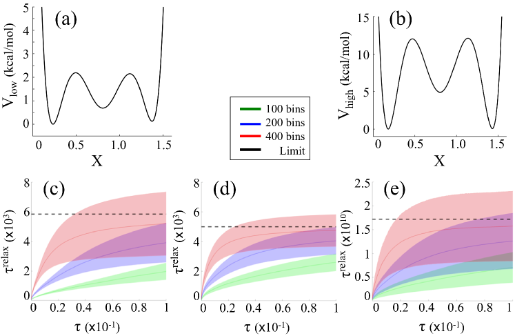
Figure 1: (a) Analytical potentials $V_{\textrm{low}}$ and (b) $V_{\textrm{high}}$ considered in the 1D Langevin simulations. The lagtime dependence of the slowest relaxation time, $\tau^{\textrm{relax}}$, in the overdamped Langevin dynamics is shown for (a) the unbiased simulations in $V_{\textrm{low}}$, (b) the biased simulations ($K=500$ kcal/mol) in $V_{\textrm{low}}$, and (c) the biased simulations ($K=500$ kcal/mol) in $V_{\textrm{high}}$ for different numbers of bins, $N_{\textrm{bin}}$. The limiting relaxation times, $\mu^{\textrm{relax}}$, obtained from Eq. 19 are shown with dashed lines for comparison. We measured $\mu^{\textrm{relax}}=5.8\times 10^{3}$, $5.1\times 10^{3}$, and $1.7\times 10^{10}$ in panels (c), (d), and (e), respectively. Uncertainties, as represented in shaded area in panels (c), (d), and (e), were estimated from 10 independent runs.

Typically, we can assess the non-Markovian effects by carrying out the Chapman-Kolmogorov test, verifying that $n$ times the lagtime of a Markov process is equivalent to raising the transition matrix to power $n$ [54]. The relaxation time of a Markovian system must then be invariant under lagtime changes. The smallest lagtime $\tau$ at which this condition is sufficiently fulfilled is called the Markov timescale, $\tau_{M}$ [6, 49].

Given the one-dimensional time series of microstates $i\in\{1,\ldots,N_{\rm bin}\}$, one can rewrite the $n$-th conditional moment in its discrete form

$$c^{(n)}(x_{i},\tau)=\sum_{j=1}^{N_{\rm bin}}(x_{j}-x_{i})^{n}~{}M_{ji}^{(\tau)}\,,$$ (8)

where $x_{i}$ is the (discretized) value of the RC in the center of bin $i$. In many cases, for a given $X$, $c^{(n)}(X,\tau)$ depends linearly on $\tau$ in the range of $\tau$ for which the diffusive regime is satisfied. Consequently the drift and diffusion coefficients are estimated solely by the quotient between the corresponding conditional moment and the lagtime $\tau$ in this range. Integrating Eq. 1 within the Taylor-Ito framework yields the stochastic Euler equation [40, 42]

$$X(t+\tau)=X(t)+D^{(1)}(X)\tau+\sqrt{D^{(2)}(X)\tau}~{}\eta(t)\,,$$ (9)

where $\eta(t)$ is a Gaussian white noise with the same average and correlation as $\Gamma(t)$. Inserting Eq. 9 into Eq. 6 yields the relations between the conditional moments and the drift and diffusion coefficients [34]

$$c^{(1)}(X,\tau) \approx D^{(1)}(X)\tau\,,$$ (10)

$$c^{(2)}(X,\tau) \approx 2D^{(2)}(X)\tau+\big{(}D^{(1)}(X)\tau\big{)}^{2}\,.$$ (11)

The latter can be subsequently assessed from the slope of a weighted polynomial regression of Eqs. 10 and 11.

Similarly to the one-dimensional case discussed above, the two-dimensional case comprehends two stochastic variables, $X(t)$ and $Y(t)$, governed by the stochastic differential equation [6, 34]

$$\frac{d}{dt}\begin{bmatrix}X\\ Y\end{bmatrix} = \begin{bmatrix}D_{1}^{(1)}(X,Y)\\ D_{2}^{(1)}(X,Y)\end{bmatrix}$$

$$+ \begin{bmatrix}g_{11}(X,Y)&g_{12}(X,Y)\\ g_{21}(X,Y)&g_{22}(X,Y)\end{bmatrix}\begin{bmatrix}\Gamma_{1}(t)\\ \Gamma_{2}(t)\end{bmatrix}\,,$$

where the drift coefficient $\textbf{D}^{(1)}=(D_{1}^{(1)},D_{2}^{(1)})^{T}$ is a two-dimensional vector and the diffusion coefficient is a $2\times 2$ matrix given by $\textbf{D}^{(2)}=\textbf{g}\textbf{g}^{T}$, with $\star^{T}$ the transpose algebraic operator. Similar to the one-dimensional case the integration of Eq. II.2 follows from a simple Euler scheme leading to

$$\begin{bmatrix}X(t+\tau)\\ Y(t+\tau)\end{bmatrix} = \begin{bmatrix}X(t)\\ Y(t)\end{bmatrix}+\tau\begin{bmatrix}D_{1}^{(1)}(X,Y)\\ D_{2}^{(1)}(X,Y)\end{bmatrix}$$

$$+ \sqrt{\tau}\begin{bmatrix}g_{11}(X,Y)&g_{12}(X,Y)\\ g_{21}(X,Y)&g_{22}(X,Y)\end{bmatrix}\begin{bmatrix}\eta_{1}(t)\\ \eta_{2}(t)\end{bmatrix}\,.$$

The trajectory data can then be analyzed with 2D MSMs [30] to construct the two-dimensional Markov transition probability matrix, $\mathbf{M}^{(\tau)}$, at lagtime $\tau$ and the respective conditional moments yielding the expression for the drift and diffusion coefficients

$$c^{(1)}(x_{i},y_{i},\tau) = \sum_{j=1}^{N_{\rm bin}}(x_{j}-x_{i})~{}M_{ji}^{(\tau)}\,,$$ (14)

$$c^{(2)}(x_{i},y_{i},\tau) = \sum_{j=1}^{N_{\rm bin}}(x_{j}-x_{i})(y_{j}-y_{i})~{}M_{ji}^{(\tau)}\,,$$ (15)

which now depend on the initial bin $i$ through the values of the two discretised RCs, $x_{i}$ and $y_{i}$. Extracting the drift and diffusion coefficients from MSMs and KM expansion depends on two parameters. The first parameter is the number of bins, $N_{\textrm{bin}}$, dividing the RC, at which $D^{(1)}$ and $D^{(2)}$ are estimated. This integer should not be too large that each bin does no longer include sufficient statistics of the transition counts and also not too small that no dependence of the drift and diffusion on the state variable can be observed [34]. The second parameter is the range of lagtimes, $\mathbf{L}_{\tau}$, used to build the Markov transition matrix $\mathbf{M}^{(\tau)}$ and calculate the KM coefficients for different $\tau$ values in Eq. 4. The conditional moments in Eq. 8 are computed for each bin and for each lagtime. For each bin, a linear fit is computed for all lagtimes in $\mathbf{L}_{\tau}$. In practice, we have to carefully consider the range of lagtimes, as too short lagtimes lead to non-Markovian effects, where the approximations for MSMs can break down. To address the choice of lagtimes, we can also consider a more extensive phase space in higher dimensions, with more finely discretized MSMs, where non-Markovian effects are reduced.

The construction of MSMs from biased simulation data has not been traditionally possible. Biased simulations modify the potential energy function of the system of interest such that the system is, for example, harmonically restrained to a given region of the energy landscape. This is advantageous as it allows sampling of regions which might otherwise not be adequately visited during the simulation time. However, the kinetic behavior observed is no longer representative of the true system, and as such, this needs to be accounted for when constructing the MSMs. Several recent numerical methods have been proposed in the literature to estimate unbiased MSMs from biased (e.g. umbrella sampling or replica exchange) MD simulations [30, 55, 36, 56, 57]. We used here the dynamic histogram analysis method (DHAM) [30], which uses a maximum likelihood estimate of the MSM transition probabilities $M_{ji}^{(\tau)}$ given the observed transition counts during each biased trajectory. The unbiased estimate $M_{ji}^{(\tau)}$ can then be inserted into Eq. 8 within the KM framework, which yields the estimation of the drift and diffusion coefficients.

III Results

In the following we give several illustrative examples of the approach presented in the Methods section. We used analytical models both in one and two dimensions within the Brownian overdamped or full inertial Langevin equations. We also used explicit solvent simulations, including the water-mediated conformations of alanine dipeptide and the permeation of the Domperidone drug molecule across a lipid membrane.

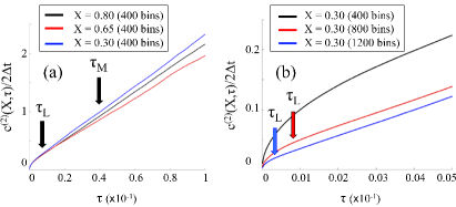
Figure 2: Evolution of $c^{(2)}(X,\tau)$ in the Brownian unbiased dynamics and $V_{\textrm{low}}$ for (a) three different position along the RC and a fixed $N_{\textrm{bin}}=400$ and (b) different values of $N_{\textrm{bin}}=400$, $800$, and $1200$ and a fixed position $X=0.30$. The value of the Markov timescale, $\tau_{M}\approx 0.04$, obtained from the analysis of the relaxation time $\tau^{\textrm{relax}}$ in Fig. 1 and $N_{\textrm{bin}}=400$ is indicated. The timescale $\tau_{L}$ indicating the departure from the linear regime of $c^{(2)}(X,\tau)$ is shown for comparaison. We measured $\tau_{L}\approx 10^{-2}$, $10^{-3}$, and $5\times 10^{-4}$ for $N_{\textrm{bin}}=400$, $800$, and $1200$, respectively.

III.1 1D Brownian overdamped Langevin equation

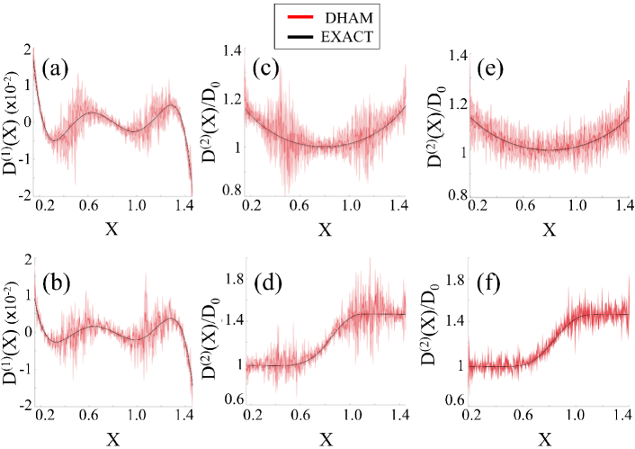
Figure 3: Top panels. Brownian dynamics simulations in $V_{\textrm{low}}$ and quadratic diffusion profile. The drift (a) and diffusion (c) profiles obtained in unbiased simulations are shown along with the diffusion profile obtained in US simulations with biasing spring constant $K=500$ kcal/mol (e). Bottom panels. Brownian dynamics simulations in $V_{\textrm{low}}$ and steplike diffusion profile. The drift (b) and diffusion (d) profiles obtained in unbiased simulations are shown along with the diffusion profile obtained in US simulations with biasing spring constant $K=500$ kcal/mol (f). The diffusion coefficients, $D^{(2)}(X)$, are rescaled to their respective minimum values defined in the main text, $D_{0}=k_{B}T/\gamma_{0}^{P}$ or $D_{0}=k_{B}T/\gamma_{0}^{Z}$, for clarity. The profiles obtained within the DHAM framework (red) agree within standard error with the exact profiles obtained from the generalization of Einstein’s relation (black). Uncertainties, as represented in shaded area, were estimated from 10 independent runs.

As a first example we integrated the 1D Brownian overdamped Langevin equation

$$\frac{dx(t)}{dt}=\frac{F(x(t))}{\gamma(x(t))}+\sqrt{\frac{k_{B}T}{\gamma(x(t))}}\eta(t)\,,$$ (16)

with $k_{B}$ the Boltzmann constant and $T=300~{}K$ the temperature of the system. In Eq. 16, the mass of the system is conveniently set to unity and $F(x)=-\nabla V(x)$ is the deterministic force derived from the 1D potential energy $V(x)=V_{\textrm{ref}}(x)+V_{\textrm{bias}}(x)$. In the following, $V_{\textrm{ref}}=\sum_{n=0}^{6}\alpha(n)x^{n}$ is defined as a polynomial of degree $6$. We considered two different choices of the coefficients $\alpha$, as detailed in the supporting information (SI), leading to the high ($V_{\textrm{high}}$) and low ($V_{\textrm{low}}$) barrier potentials plotted in Fig. 1(a) and (b), respectively. The biased potential is defined as $V_{\textrm{bias}}=\frac{1}{2}K\big{(}x-x^{(k)}\big{)}^{2}$ with $K$ the biasing spring constant and $x^{(k)}$ the center of the harmonic bias in simulation $k$. The parameter $\gamma(x)$ represents the position-dependent friction coefficient with $D(x)=k_{B}T/\gamma(x)$ the natural generalization of Einstein’s relation defining the position-dependent diffusion coefficient [45]. We used the Itô convention to obtain the first order integrator of the overdamped Langevin equation [40, 42]. The total number of timesteps $N_{\textrm{step}}$ in the unbiased or biased simulation runs was chosen such that the simulation time $\Delta t\times N_{\textrm{step}}=5\times 10^{4}$ was kept constant. The simulation timestep was set to $\Delta t=10^{-5}$, which is at least an order of magnitude smaller than the slow characteristic time scale for the diffusion in the system, $\tau_{\textrm{diff}}=1/\max_{x}\big{(}\gamma(x)\big{)}$.

Unbiased simulation. We studied the evolution of the system under Eq. 16 with the low barrier analytical potential $(V_{\textrm{low}})$ shown in Fig. 1(a) and $V_{\textrm{bias}}=0$. We considered either a quadratic or step-like position-dependent diffusion profile with $\gamma(x)$ a parabolic (P) or a $Z$-shaped membership (Z) function [58],

$$\gamma^{P}(x) = \gamma_{0}^{P}\Big{(}1-\frac{1}{3}(x-x_{P})^{2}\Big{)}\,,$$ (17)

$$\gamma^{Z}(x) = \gamma_{0}^{Z}\Big{(}2+\textrm{zmf}(x,a,b)\Big{)}\,,$$ (18)

with $\gamma_{0}^{P}=3000$, $x_{P}=0.8$, $\gamma_{0}^{Z}=1700$, $a=0.5$, $b=1.1$, and $\textrm{zmf}(x,a,b)$ the sigmoidal membership function (see details in the SI). We first assessed the Markov timescale $\tau_{M}$ associated with the trajectories generated via Eq. 16 for different binning $N_{\textrm{bin}}=100$, $200$, and $400$, via the Chapman-Kolmogorov test. Then, we inferred the relaxation time of the system, in the limit of very long lagtimes, using the fitting procedure introduced in previous work [53], which describes the relaxation time, $\tau^{\textrm{relax}}$, as

$$\tau^{\textrm{relax}}=\frac{\tau\times\mu^{\textrm{relax}}}{\tau+\epsilon\mu^{\textrm{relax}}}\,.$$ (19)

In Eq. 19, $\tau$ is the lagtime, and $\mu^{\textrm{relax}}$ and $\epsilon$ are two free parameters which represent the true (limiting) relaxation timescale and the initial rate of change of the effective relaxation time, respectively. As shown in Fig. 1(c), increasing moderately the number of bins from $100$ to $400$ increases the rate of convergence towards the true relaxation time, $\mu^{\textrm{relax}}=5.8\times 10^{3}$, obtained from Eq. 19 with $N_{\textrm{bin}}=400$. We obtained similar values for the true relaxation times measured with $N_{\textrm{bin}}=200$ and $100$ (data not shown). This yields a smaller Markov timescale, $\tau_{M}$, which, in turn, gives a more accurate measure of the drift and diffusion coefficients, in line with the variational principle satisfied by the MSMs [59]. Increasing further $N_{\textrm{bin}}$, however, each bin would eventually no longer include the requisite sufficient statistics for the MSM analysis. Considering $N_{\textrm{bin}}=400$ in Fig. 1(c), the relaxation time can be seen to level off in the region of lagtimes greater than $0.2$. In the analysis that follows, we chose to define $\tau_{M}\approx 0.4$, as it is sufficiently large to be insensitive to the precise choice of the lagtime. Subsequently, the first and second conditional moments were evaluated using Eq. 4 over the range of lagtime $\tau\geq\tau_{M}$.

In Fig. 2(a) and (b), the representative evolution of $c^{(2)}(X,\tau)$ is shown for different positions along the RC and different number of bins, respectively. At relatively long lagtime, for $\tau\geq\tau_{M}$, $c^{(2)}$ follows the linear trend expected from Eq. 11. Close analysis of the evolution of $c^{(2)}$ shows that the linear trend is satisfied above a lagtime threshold, $\tau_{L}$, significantly lower than $\tau_{M}$. At sufficiently short lagtime, on the other hand, for $\tau<\tau_{L}$, $c^{(2)}$ deviates from the linear trend, which stems from non-Markovian effects coming from the system discretization. As shown in Fig. 2(b), increasing the number of bins from $N_{\textrm{bin}}=400$ to $1200$ decreases the value of the lagtime threshold, $\tau_{L}$, above which the linear trend obtained in Eq. 11 is satisfied.

Drift and diffusion coefficients were subsequently assessed from the slope of a weighted polynomial regression following Eqs. 10 and 11. We also calculated the fourth-order coefficient and evaluated the ratio $D^{(4)}(X)/\big{(}D^{(2)}(X)\big{)}^{2}<5\times 10^{-3}$, indicating the validity of the condition of the Pawula theorem. As shown in Fig. 3(a)-(d), we observed excellent agreement between the theoretical profiles and the numerical results for both position-dependent drift and diffusion coefficients, with higher variability around $X\approx 0.5$ and $\approx 1.2$, where the derivative of the low barrier potential $V_{\textrm{low}}$, shown in Fig. 1(a), is maximal.

Biased simulation. We extented the previous analysis to the biased evolution of the system in the low $(V_{\textrm{low}})$ and high $(V_{\textrm{high}})$ barrier potentials shown in Figs. 1(a) and (b), respectively, within the US framework. We ran standard US simulations with the biasing potential $V_{\textrm{bias}}$ defined above in each umbrella window. We used $50$ uniformly distributed umbrella windows in the range $[0.25,1.35]$ along the RC. This number was sufficiently high to obtain accurate sampling, given the different biasing spring constants considered in this work.

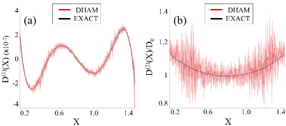
Figure 4: Drift (a) and diffusion (b) profiles obtained in biased overdamped Langevin simulations for the high energy barrier potential ($V_{\textrm{high}}$). A biasing spring constant $K=500$ kcal/mol and a quadratic diffusion profile are used. The diffusion coefficient $D^{(2)}(X)$ is rescaled to $D_{0}=k_{B}T/\gamma_{0}^{P}$ for clarity. The profiles obtained within the DHAM framework (red) agree within standard error with the exact profiles obtained from the generalization of Einstein’s relation (black). Uncertainties, as represented in shaded area, were estimated from 10 independent runs.

We first studied the effect of the bias on the reconstruction of the diffusion coefficient when the system evolves in $V_{\textrm{low}}$. We set the biasing spring constant to $K=500$ kcal/mol, which was sufficienlty strong to allow good sampling in both low ($V_{\textrm{low}}$) and high ($V_{\textrm{high}}$) barrier potentials. The lagtime dependence of $\tau^{\textrm{relax}}$ is shown in Fig. 1(d). We observed a similar behaviour to the one obtained in the unbiased simulations (Fig. 1(c)) with the decline of the non-Markovian effects on the dynamics when the number of bins, $N_{\textrm{bin}}$ increases from $100$ to $400$. Most noticeably, the use of the biasing spring constant decreases significantly the variability of the relaxation timescale at longer lagtimes. As shown in Figs. 3(e) and (f), excellent agreement is observed between the theoretical profiles and the numerical results. We also confirmed that $D^{(4)}(X)/\big{(}D^{(2)}(X)\big{)}^{2}<5\times 10^{-3}$. As expected, the use of the biasing spring constant yields better sampling across the RC.

We complemented this analysis with the reconstruction of the diffusion coefficient of the system using $V_{\textrm{high}}$ and a biaising spring constant $K=500$ kcal/mol. The relaxation timescale is shown in Fig. 1(e). We observed a similar behavior to the unbiased simulations with the decline of the non-Markovian effects on the dynamics when the number of bins, $N_{\textrm{bin}}$ increases from $100$ to $400$. The relaxation time of the system calculated for $N_{\textrm{bin}}=400$ converges towards a limiting value, $\mu^{\textrm{relax}}=1.7\times 10^{10}$, significantly higher than the one measured for $V_{\textrm{low}}$, due to the longer equilibration time needed to cross the high energy barrier. As shown in Figs. 4(a) and (b), we observed good agreement between the theoretical profiles and the numerical results for the drift and diffusion coefficients. We also verified that $D^{(4)}(X)/\big{(}D^{(2)}(X)\big{)}^{2}<5\times 10^{-3}$. We noticed, however, higher variability around $X\approx 0.5$ and $\approx 1.2$, where the derivative of the high barrier potential $V_{\textrm{high}}$ (Fig. 1(b)) is maximal. As shown in the SI, the increase of the biasing spring constant from $500$ kcal/mol to $2000$ kcal/mol yields better sampling around the transition states with lower variability on the reconstruction of the diffusion profile, as already observed in the low barrier case.

III.2 1D full inertial Langevin equation

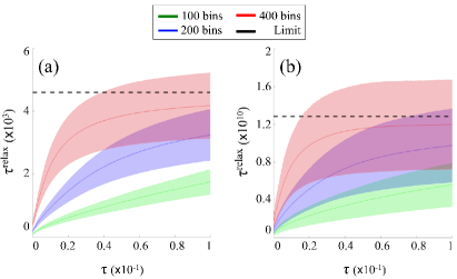
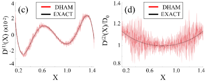
Figure 5: Relaxation times $\tau^{\textrm{relax}}$ as a function of the lagtime, $\tau$, and the number of bins, $N_{\textrm{bin}}$, obtained in biased 1D full Langevin simulations for (a) low barrier ($V_{\textrm{low}}$) and (b) high barrier ($V_{\textrm{high}}$) energy potentials. A biasing spring constant $K=500$ kcal/mol is used. Drift (c) and diffusion (d) obtained for US simulations with biasing spring constant $K=500$ kcal/mol and quadratic diffusion profile. The diffusion coefficient $D^{(2)}(X)$ is rescaled to $D_{0}=k_{B}T/\gamma_{0}^{P}$ for clarity. The profiles obtained within the DHAM framework (red) in panels (c) and (d) agree within standard error with the exact profiles obtained from the generalization of Einstein’s relation (black). Uncertainties, as represented in shaded area, were estimated from 10 independent runs.

To take into account the role played by inertia in the reconstruction of the drift and diffusion coefficients, we extended Eq. 16 to the full inertial Langevin equation

$$\frac{d^{2}x(t)}{dt^{2}}=F(x(t))-\gamma(x(t))\frac{dx(t)}{dt}+\sqrt{k_{B}T\gamma(x(t))}\eta(t)\,,$$ (20)

where the mass of the system is conveniently set to unity. From this relation, we used the Vanden-Eijnden and Ciccotti algorithm [60] that generalises the Velocity Verlet integrator to Langevin dynamics, along with the Itô convention. This scheme takes the inertial term into account and is accurate to order $\Delta t^{2}$.

We used the same simulation timestep, $\Delta t=10^{-5}$, and biasing spring constants, $K=500$ kcal/mol, as in the Brownian overdamped Langevin dynamics. The lagtime dependence of the relaxation time $\tau^{\textrm{relax}}$, as shown in Fig. 5(a) and (b) for $V_{\textrm{low}}$ and $V_{\textrm{high}}$, respectively, is similar to the one measured in the Brownian overdamped Langevin simulation, with the decline of the non-Markovian effects when the number of bins, $N_{\textrm{bin}}$ increases from $100$ to $400$, and the convergence towards the limiting relaxation times $\mu^{\textrm{relax}}=4.4\times 10^{3}$ and $1.3\times 10^{10}$ for $V_{\textrm{low}}$ and $V_{\textrm{high}}$, respectively, calculated for $N_{\textrm{bin}}=400$.

We limited the rest of the analysis to the biased evolution of the system in $V_{\textrm{high}}$. The associated drift and diffusion profiles are shown in Fig. 5(c) and (d) (see details in the SI). We observed good agreement between theoretical and numerical profiles, with $D^{(4)}(X)/\big{(}D^{(2)}(X)\big{)}^{2}<4\times 10^{-3}$. As already noted in the overdamped Langevin dynamics, we observed higher variability around $X\approx 0.5$ and $\approx 1.2$, where the derivative of the potential energy $V_{\textrm{high}}$ is maximal. Increasing the biasing spring constant from $K=500$ kcal/mol to $2000$ kcal/mol improved the accuracy of the measure of the diffusion coefficient (Fig. S2).

III.3 2D Brownian overdamped Langevin equation

We extended the 1D analysis above to the estimation of the 2D diffusion tensor of the analytical system evolving under the 2D Brownian overdamped equation [61]

$$\gamma(t)\frac{d\mathbf{X}}{dt}=\mathbf{F}(\mathbf{X})+\sqrt{k_{B}T}~{}\mathbf{b}(t)~{}\eta(t)$$ (21)

where $\mathbf{X}\equiv\big{(}X,Y\big{)}$ is a 2D vector and $\textbf{F}(\mathbf{X})=-\nabla V(\mathbf{X})$ is the deterministic force derived from the 2D potential energy $V(\mathbf{X})$. In Eq. 21, the force $\textbf{b}(t)$ is related to the friction tensor $\mathbf{\gamma}(t)$ as follows

$$\mathbf{\gamma}(t)=\textbf{b}(t)\textbf{b}^{T}(t)\,,$$ (22)

and $\eta(t)=\big{(}\eta_{1}(t),\eta_{2}(t)\big{)}$ is a 2D vector of independent, identical Gaussian white noise sources, i.e. $\langle\eta_{i}(t)\rangle=0$ and $\langle\eta_{i}(t)\eta_{j}(t^{\prime})\rangle=2\delta_{i,j}\delta(t-t^{\prime})$. From this relation, we used the Itô convention to obtain the first order integrator of Eq. 21. For economy of computational resources, we focused our analysis on a diagonal friction tensor

$$\gamma(t)=\begin{bmatrix}\gamma_{11}(\mathbf{X})&0\\ 0&\gamma_{22}(\mathbf{X})\end{bmatrix}$$ (23)

with constant friction $\gamma_{11}(\mathbf{X})=300$ and $\gamma_{2}(\mathbf{X})=30$ and the 2D analytical potential $V(\mathbf{X})=-3X^{2}+X^{4}-3XY+Y^{4}$ shown in Fig. 6(a). We modeled standard US simulations, evenly positioned along the RC, with a 1D bias potential $V_{\textrm{bias}}(\mathbf{X})=V^{(k)}(X)=\frac{1}{2}K(X-X^{(k)})^{2}$ in each umbrella window $k$, with $K$ the biasing spring constant and $X^{(k)}$ the center of the harmonic bias in window $k$. We used $50$ uniformly distributed umbrella windows in the range $[0.25,1.35]$ along the $x$-axis. We then constructed a discretized 2D grid to determine the MSMs along the $x$- and $y$-axes.

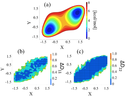
Figure 6: (a) Free-energy surface associated with the 2D analytical model potential projected along the $x$- and $y$-axes. The 2D projections of the deviation of the numerical diagonal elements of the diffusion tensor, $\Delta D_{11}$ and $\Delta D_{22}$, are shown in panels (b) and (c), respectively.

The diagonal elements of the diffusion tensor were obtained from the analysis of the KM coefficients defined in Eqs. 14 and 15 (see details in the SI). We also calculated the fourth-order coefficients and verify that the ratio $D_{11}^{(4)}(X)/\big{(}D_{11}^{(2)}(X)\big{)}^{2}<5\times 10^{-3}$ and $D_{22}^{(4)}(X)/\big{(}D_{22}^{(2)}(X)\big{)}^{2}<6\times 10^{-4}$, indicating the validity of the condition of the Pawula theorem. To assess the accuracy of the reconstructed diffusion coefficient, we measured the deviation between the observed (ob) and theoretical (th) values

$$\Delta D_{ii}(\mathbf{X})=\frac{\big{|}D_{ii}^{(\textrm{ob})}(\mathbf{X})-D_{ii}^{(\textrm{th})}(\mathbf{X})\big{|}}{D_{ii}^{(\textrm{th})}(\mathbf{X})}\,,$$ (24)

with $D_{ii}^{(\textrm{th})}(\mathbf{X})=k_{B}T/\gamma_{ii}(\mathbf{X})$. In Fig. 6(b) and (c), it is shown the numerical measures for $\Delta D_{11}(\mathbf{X})$ and $\Delta D_{22}(\mathbf{X})$, respectively. The observations are in good agreement with the theoretical values $D_{11}^{\textrm{th}}(\mathbf{X})=2\times 10^{-3}$ and $D_{22}^{\textrm{th}}(\mathbf{X})=2\times 10^{-2}$. Most noticeably, the lower value of the friction parameter $\gamma_{22}(\mathbf{X})$ allows better sampling, which yields a more accurate measure for $D_{22}(\mathbf{X})$. Finally, to quantify the accuracy of the reconstruction, we measured the effective diffusion coefficient along each reaction coordinate

$$D_{ii}^{\textrm{eff}}=\frac{1}{N_{\textrm{bin}}}\int D_{ii}(\mathbf{X})~{}d\mathbf{X}\,.$$ (25)

We measured $D_{11}^{\textrm{eff}}=(1.9\pm 0.4)\times 10^{-3}$ and $D_{22}^{\textrm{eff}}=(2.0\pm 0.7)\times 10^{-2}$, in good agreement with $D_{11}^{\textrm{th}}$ and $D_{22}^{\textrm{th}}$, respectively.

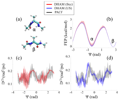
Figure 7: (a) Ball-and-stick representation of the conformers $\alpha$ and $\beta$ of Ala2 along with (b) the free energy profile reconstructed along the dihedral angle $\Psi$ $(N1-C\alpha-C2-N2)$ using the DHAM in unbiased (red) and biased (blue) simulations. The diffusion profiles obtained in (c) unbiased and (d) biased simulations agree within standard errors with the one obtained within the PACF method of Hummer (grey) [4]. Uncertainties, as represented in shaded areas, were estimated from 3 independent runs.

III.4 Water-mediated conformations of Alanine Dipeptide in 1D

The conformational transition between the different conformers of the solvated alanine dipeptide (Ala2) has been extensively used as a case study for several theoretical and computational investigations [62, 63, 64, 65, 66, 14]. We studied the transition between the metastable states $\alpha$ and $\beta$ of Ala2 shown in Fig. 7(a), which can be differenciated by the values of the backbone dihedral angle $\Psi$ and are separated by an activation free energy barrier of $\approx 2$ kcal/mol at the temperature $T=300~{}K$. We used a Langevin thermostat to enforce the temperature [67], a time step of $0.2$ fs, AMBER03 force field [68] with TIP3P water model [69], and GROMACS 5.1 molecular dynamics code [70]. A single alanine dipeptide molecule was kept in a solvated periodic cubic box of edge $\approx 3$ nm. The LINear Constraint Solver (LINCS) algorithm [71] handled bond constraints while the particle-mesh Ewald scheme [72] was used to treat long-range electrostatic interactions. The non-bonded van der Waals cutoff radius was $0.8$ nm.

The relatively low energy barriers allow the system to be sampled with both unbiased and biased simulations, which gives a mean to assess the accuracy of the results obtained with enhanced sampling methods. We determined the free energy profile and diffusion coefficient by using either free simulations ($500$ ns) or US biased simulations and the DHAM approach. The starting structures for the US simulations were obtained by pulling the system along the dihedral angle $\Psi$ within the range $[-\pi,\pi]$. During the simulations, a snapshot was saved every $0.1$ rad generating $60$ windows. Each US window was subsequently run for $1$ ns to allow equilibration, followed by additional $5$ ns of the production run using an US force constant of $5$ kcal $\textrm{mol}^{-1}$ $\textrm{rad}^{-2}$. In Fig. 7(b), (c), and (d) are shown the reconstructed FEPs and diffusion coefficients obtained within the DHAM framework, either with unbiased (red) or biased (blue) simulations. Both approaches gave similar results. In particular, we compared the diffusion profiles obtained with DHAM with the one obtained within the PACF framework (grey),

$$D(\Psi_{k}=\langle\Psi\rangle_{k})=\frac{\textrm{var}(\Psi)^{2}}{\int_{0}^{\infty}C_{\Psi}(t)~{}dt}~{}.$$ (26)

In Eq. 26, $\langle\Psi\rangle_{k}$ is the average of the RC in the US window $k$, $\textrm{var}(\Psi)=\langle\Psi^{2}\rangle-\langle\Psi\rangle^{2}$ is its variance, and $C_{\Psi}(t)=\langle\delta\Psi(0)\delta\Psi(t)\rangle$ the PACF calculated directly from the time series. Following the original work of Hummer, we increased the strength of the biasing potential from $\approx 5$ kcal $\textrm{mol}^{-1}$ $\textrm{rad}^{-2}$ to $\approx 24$ kcal $\textrm{mol}^{-1}$ $\textrm{rad}^{-2}$ to satisfy the underlying assumption that the harmonic restraint be sufficiently large to render the underlying free energy surface a small perturbation on the harmonic potential [4]. As shown in Fig. 7(c) and (d), we observed good agreement between the results derived with DHAM either in the unbiased or biased simulations and the PACF method. To compare the results with those in the literature, we measured the effective diffusion coefficient

$$D^{(2)}_{\textrm{eff}}=\frac{1}{N_{\textrm{bin}}}\int_{-\pi}^{+\pi}D^{(2)}(\Psi)~{}d\Psi\,.$$ (27)

with $N_{\textrm{bin}}$ the number of bins used in the MSM. Eq. 27 yields the effective Diffusion coefficient $D^{(2)}_{\textrm{eff}}\approx 0.16~{}\textrm{rad}^{2}/\textrm{ps}$, in agreement with the result obtained by Hummer et al. [73, 4] ($\approx 0.15~{}\textrm{rad}^{2}/\textrm{ps}$) and Ma et al. [5] ($\approx 0.34~{}\textrm{rad}^{2}/\textrm{ps}$).

III.5 Membrane permeation in 1D

In this section we applied our method to study the permeation of Domperidone, a dopamine receptor antagonist, across a POPC lipid membrane [74, 75, 11], as illustrated in Fig. 8(a). The simulation data were obtained from previous studies [75, 11] and further details of the simulation methods and parameters can be found there. This system shows long time scale fluctuations inherent to the presence of the bilayer structure, which is representative of the transport of solute across heterogeneous media [75]. As described in the original work of Dickson et al. [75], the starting structures for the US simulations were obtained by placing the ligand at the center of a POPC bilayer surrounded by water molecules ($72$ POPC and $60$ waters per lipid). To generate the US windows, the drug was pulled out from the center of the system to outside the membrane, for a total of $40~{}\textrm{\AA}$. Configurations were saved every $1~{}\textrm{\AA}$, from the center $z=0~{}\textrm{\AA}$ to $z=40~{}\textrm{\AA}$ generating $40$ windows. Each US window was run for $20$ ns to allow equilibration, followed by additional $80$ ns of the production run using an US force constant of $2.5~{}\textrm{kcal}~{}\textrm{mol}^{-1}\textrm{\AA}^{-2}$.

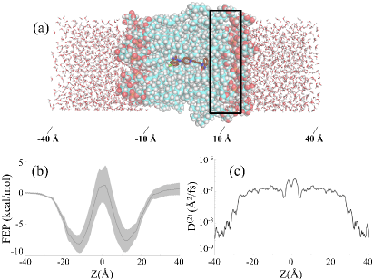
Figure 8: (a) Schematic representation of Domperidone (in brown at the center of the image) at the center of a POPC bilayer surrounded by water. The local area centered around $Z=10\AA$, considered in the 2D calculation of the diffusion tensor, is shown (solid black rectangle). (b) Free energy and (c) diffusion profiles (in semi-log representation) associated with the crossing of the drug molecule through the bilayer and reconstructed along the distance from the center of the bilayer, $Z$. Uncertainties, as represented in shaded area, were determined by dividing the data into $5$ equal sections.

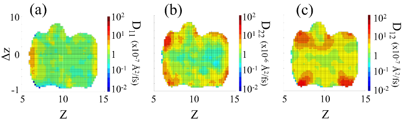
Figure 9: 2D projection of the diagonal (a-b) and off-diagonal (c) elements of the diffusion tensor, $D_{11}(Z,\Delta z)$, $D_{22}(Z,\Delta z)$, and $D_{12}(Z,\Delta z)$, associated with the crossing of Domperidone across the POPC membrane bilayer. We restrained the exploration of the free energy landscape to the area centered around the minimal energy well ($Z\approx 10\textrm{\AA}$ in Figs. 8(a) and (b)).

The FEP and the diffusion profiles associated with the transport of Domperidone across the POPC bilayer, as shown in Fig. 8(b) and (c), respectively, were obtained using the DHAM. As the drug reaches the water/bilayer interface, the value of the diffusion coefficient significantly increases before remaining approximately constant until the molecule reaches the adjoining area of the two lipid layers, which is representative of the hydrophobic nature of the compound. These results can be interpreted within the inhomogeneous solubility-diffusion model commonly used to provide realistic description of membrane permeation [76]. In this model, the permeability, Perm, is written as

$$\frac{1}{\textrm{Perm}}=\int_{-d/2}^{+d/2}\frac{1}{K(Z)D(Z)}=\int_{-d/2}^{+d/2}\frac{\exp\big{(}\Delta G(Z)/k_{B}T\big{)}}{D(Z)}~{},$$ (28)

where $K(Z)$, $D(Z)$, and $d$ are the position-dependent partition coefficient, the solute diffusion coefficient, and the membrane thickness respectively. $\Delta G(Z)$ is the free energy difference, which is related to the partition coefficient $K(Z)=\exp\big{(}-\Delta G(Z)/k_{B}T\big{)}$. Considering the results shown in Fig. 8, we obtained the $\log$ Perm value associated with the transport of the Domperidone molecule across the POPC bilayer, $\log\textrm{Perm}=-2.71\pm 0.15$, which is in agreement with experimental results ($\log\textrm{Perm}^{(\textrm{exp})}=-2.6$) [74, 75, 11].

III.6 Membrane permeation in 2D

We extended the 1D study above to the 2D analysis of the permeation of Domperidone across the POPC lipid membrane. To do so, we considered the rotational movement of the drug during its passage across the membrane as additional degree of freedom. We constructed a discretized two-dimensional grid to determine the MSMs along two reaction coordinates (see details in the SI). As our first reaction coordinate, we used the distance from the drug center of mass to bilayer center, $Z$, as already considered in 1D. For our second coordinate, we used the projection of the molecular orientation vector onto the axis orthogonal to the bilayer axis, $\Delta Z$, as a measure of the orientation of the drug with respect to the membrane, as described in Badaoui et al. [11]. We restrained the exploration of the free energy landscape to the area centered around the minimal energy well ($Z\approx 10\textrm{\AA}$ in Figs. 8(a) and (b)). We measured the diagonal and off-diagonal KM coefficients defined in Eqs. 14 and 15 (see details in the SI). Subsequently, the associated elements of the diffusion tensor were obtained with weighted polynomial regression.

In Fig. 9(a), (b), and (c), we calculated the 2D projection of the diagonal and off-diagonal elements of the diffusion tensor, $D_{11}(Z,\Delta z)$, $D_{22}(Z,\Delta z)$, and $D_{12}(Z,\Delta z)$, respectively. We observed good agreement in the order of magnitude between the measure of $D_{11}(Z,\Delta z)$ (Fig. 9(a)) and the one of $D^{(2)}(Z)$ (Fig. 8(c)) in the minimal energy well. Additionally, we measured that the orientation of the drug with respect to the membrane diffuses an order of magnitude faster than the drug COM through the bilayer. Finally, we estimated the off-diagonal element of the diffusion tensor, which is essential for understanding the importance of dynamic coupling between the coordinates. As shown in Fig. 9(c), the order of magnitude of $D_{12}(Z,\Delta z)$ is comparable to the one measured for $D_{11}(Z,\Delta z)$ and $D_{22}(Z,\Delta z)$.

IV Conclusion

In the present study, we presented a general, automatic method for estimating multi-dimensional position-dependent diffusion coefficients equally valid in biased or unbiased MD simulations. We combined Markov State Model analysis and Kramers-Moyal expansion to link the underlying stochastic process obtained within the non-linear Langevin framework to its probabilistic description. Our approach neither requires prior assumptions regarding the form of the free energy landscape nor additional numerical integration scheme. We applied our numerical approach to one- and two-dimensional analytic potentials and data from explicit solvent molecular dynamics simulations, including the water-mediated conformations of the alanine dipeptide.

Importantly, we demonstrated the efficiency of our algorithm in studying the transport of solute across three-dimensional heterogeneous porous media, which is known to show long time scale fluctuations potentially breaking ergodicity in sampling [9]. Specifically, our algorithm provided accurate assessment of the diffusion coefficient associated with the crossing of Domperidone across a lipid POPC membrane, which was not previously accessible with standard methods [75].

The method would also allow the measure of the off-diagonal elements of the diffusion tensor, which is essential for assessing the importance of dynamic coupling between the reaction coordinates. As discussed by Ma and coworkers [5], the presence of significant off-diagonal element in the diffusion tensor could indeed impact the determination of the reactive eigenvector at play in the Kramers’ theory of reaction kinetics and then the measure of the rate associated with the kinetic evolution of the system. This is particularly important in toxicology and pharmacology, where the prediction of kinetic quantities of solutes, including drugs and small peptides provides fundamental understanding of numerous biochemical transport processes involved in the design of new drugs [77].

V Acknowlegments

We acknowledge use of the research computing facility at King’s College London, Rosalind (https://rosalind.kcl.ac.uk). F.S. and E.R. thanks Gerhard Hummer for fruitful discussions and Magd Badaoui for his help in setting up the membrane bilayer system. We acknowledge the support of the UK Engineering and Physical Sciences Research Council (EPSRC), under grant number EP/R013012/1, and ERC project 757850 BioNet.

Assessing Position-Dependent Diffusion from Biased Simulations and Markov State Model Analysis

Supporting Information

1D Langevin Dynamics

Analytical Potentials. In the model systems evolving under the Brownian overdamped and the full inertial limit of the Langevin equation in 1D, the deterministic force, $F(x)=-\nabla V(x)$, in Eqs. 14 and 18 in the main text derives from the potential energy $V(x)=V_{\textrm{ref}}(x)+V_{\textrm{bias}}(x)$, where $V_{\textrm{ref}}=\sum_{n=0}^{6}\alpha(n)x^{n}$, is defined as a polynomial of degree $6$, with parameters $\alpha(n)$ given below for the low ($V_{\textrm{low}}$) and high ($V_{\textrm{high}}$) energy barrier potentials:

$V_{\textrm{ref}}$	$\alpha(0)$	$\alpha(1)$	$\alpha(2)$	$\alpha(3)$	$\alpha(4)$	$\alpha(5)$	$\alpha(6)$
$V_{\textrm{low}}$	$22.7498$	$-301.374$	$1.3865\times 10^{3}$	$-2.9683\times 10^{3}$	$3.2173\times 10^{3}$	$-1.7111\times 10^{3}$	$354.3680$
$V_{\textrm{high}}$	$47.2598$	$-722.6061$	$3.8067\times 10^{3}$	$-8.7222\times 10^{3}$	$9.7780\times 10^{3}$	$-5.2710\times 10^{3}$	$1.0919\times 10^{3}$

The biased energy potential, $V_{\textrm{bias}}=\frac{1}{2}K\big{(}x-x^{(k)}\big{)}^{2}$ is defined as an harmonic potential with $K$ the biasing spring constant and $x^{(k)}$ the center of the harmonic bias in simulation $k$, uniformly distributed along the reaction coordinate (RC).

Analytical Diffusion coefficients. We considered either a quadratic or step-like position-dependent diffusion profile, $D(x)=k_{B}T/\gamma(x)$ defined by the generalization of Einstein’s relation, with $k_{B}$ the Boltzmann constant, $T=300$ K the temperature of the system, and $\gamma(x)$ the position-dependent friction defined as a parabolic (P) or a $Z$-shaped membership (Z) function,

$$\gamma^{P}(x) = \gamma_{0}^{P}\Big{(}1-\frac{1}{3}(x-x_{P})^{2}\Big{)}\,,$$ (S1)

$$\gamma^{Z}(x) = \gamma_{0}^{Z}\Big{(}2+\textrm{zmf}(x,a,b)\Big{)}\,,$$ (S2)

with $\gamma_{0}^{P}=3000$, $x_{P}=0.8$, $\gamma_{0}^{Z}=1700$, $a=0.5$, $b=1.1$. The function $\textrm{zmf}(x,a,b)$ represents the sigmoidal membership function defined as

$$\textrm{zmf}(x,a,b)=\left\{\begin{array}[]{ll}1\,,&x\leq a\\ 1-2\Big{(}\frac{x-a}{b-a}\Big{)}^{2}\,,&a\leq x\leq\frac{a+b}{2}\\ 2\Big{(}\frac{x-b}{b-a}\Big{)}^{2}\,,&\frac{a+b}{2}\leq x\leq b\\ 0\,,&x\geq b\end{array}\right.$$

Biased 1D Langevin dynamics in $V_{\textrm{high}}$. We considered the biased evolution of the system in the high $(V_{\textrm{high}})$ barrier potential defined above, within the umbrella sampling framework. We studied the effect of increasing the biasing spring constant, $K$, from $500$ kcal/mol to $2000$ kcal/mol, on the reconstruction of the diffusion profile. We first evaluated the second conditional moments $c^{(2)}$, defined in Eq. $4$ in the main text, as shown in Fig. S1. The diffusion coefficient was subsequently assessed from the slope of a weighted polynomial regression. As shown in Fig. S2, we observed excellent agreement between the theoretical profiles and the numerical results. For the lowest biasing spring constant, $K=500$ kcal/mol, we oberved higher variability around the transition states $X\approx 0.5$ and $\approx 1.2$, as shown in Fig. S2 (a). Increasing the biasing spring constant, $K$, from $500$ kcal/mol to $2000$ kcal/mol, yields better sampling around the transition states, with lower variability on the reconstruction of the diffusion profile around the transition states, as shown in Fig. S2 (b).

Figure S1: Evolution of $c^{(2)}(X,\tau)$ in the biased full inertia Langevin dynamics and $V_{\textrm{high}}$ for three different position along the RC. The discretization of the system considered here was $N_{\textrm{bin}}=400$.

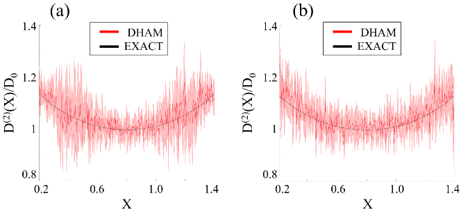
Figure S2: Diffusion profiles obtained with biased full inertia Langevin simulations in $V_{\textrm{high}}$ and quadratic diffusion when the biasing spring constant $K=500$ kcal/mol (a) and $K=2000$ kcal/mol (b). The Diffusion coefficient $D^{(2)}(X)$ is rescaled to $D_{0}=k_{B}T/\gamma_{0}^{P}$ for clarity. The discretization of the system considered here was $N_{\textrm{bin}}=400$. The profiles obtained within the DHAM framework (red) agree within standard error with the exact profiles obtained from the generalization of Einstein’s relation (black). Uncertainties, as represented in shaded area, were estimated from 10 independent runs, determining the profiles independently, and calculating the standard error.

2D Langevin Dynamics

Analogously to the 1D case, we constructed a finely discretized 2D grid to determine the MSMs along the two RC $X$ and $Y$ using the 2D-DHAM method. We considered a 2D binning of $90\times 90$, sufficiently small to measure accurately the diagonal elements of the diffusion tensor, $D_{11}$ and $D_{22}$, shown in Fig. 6 in the main text. To do so, we first evaluated the diagonal conditional moments, $c_{XX}$ and $c_{YY}$, defined in Eq. $13$ in the main text, as shown in Figs. S3 (a) and (b), respectively. The diffusion coefficient was subsequently assessed from the slope of a weighted polynomial regression.

Figure S3: Evolution of the diagonal conditional moments $c_{XX}^{(2)}$ (a) and $c_{YY}^{(2)}$ (b) in the biased Brownian overdamped Langevin dynamics in 2D, for two different positions in the potential energy surface $(X,Y)=(1.5,1.0)$ and $(X,Y)=(0,0)$ and $N_{\textrm{bin}}=90\times 90$.

Water-mediated conformations of Alanine Dipeptide in 1D

Figure S4: Evolution of (a) the slowest relaxation time, $\tau^{\textrm{relax}}$, and (b) the conditional moment $c^{(2)}$ for different values of the dihedral angle $\Psi$ measured for $N_{\textrm{bin}}=1000$. Uncertainties, as represented in shaded area, were estimated from 3 independent runs, determining the profiles independently, and calculating the standard error.

To obtain the diffusion profile associated with the conformational transition between the metastable states $\alpha$ and $\beta$ of ALA2 shown in Fig. 7 in the main text, we assessed the Markov timescale $\tau_{M}$ associated with the MD trajectory for a discretization $N_{\textrm{bin}}=1000$ (Fig. S4 (a)). We compared our results with those obtained with a different discretization $N_{\textrm{bin}}=500$, which did not show significant changes (data not shown). We then evaluated the second conditional moments, $c^{(2)}$, over the range of lagtime $\tau\geq\tau_{M}$, as shown in Fig. S4 (b). The diffusion coefficient was assessed from the slope of a weighted polynomial regression. We calculated the fourth-order coefficient and check the ratio $D^{(4)}(X)/\big{(}D^{(2)}(X)\big{)}^{2}<10^{-2}$, indicating the necessary condition of the Pawula theorem holds.

Membrane permeation

To obtain the 1D diffusion profile associated with the permeation of Domperidone, a dopamine receptor antagonist, across the lipid (POPC) membrane shown in Fig. 8 in the main text, we first assessed the Markov timescale $\tau_{M}$ associated with the MD trajectory for a discretization $N_{\textrm{bin}}=1000$ (Fig. S5 (a)). The relaxation time can be seen to level off in the region of lagtimes greater than 100 ps, where it is sufficiently large for the relaxation time to be insensitive to the precise choice of the lagtime, as shown in Fig. S5 (a). We then evaluated the second conditional moments $c^{(2)}$ defined in Eq. $4$ in the main text over the range of lagtime $\tau\geq\tau_{M}$, as shown in Fig. S5 (b). The diffusion profile, as shown in Fig. S6, was subsequently assessed from the slope of a weighted polynomial regression. We calculated the fourth-order coefficient and check the ratio $D^{(4)}(X)/\big{(}D^{(2)}(X)\big{)}^{2}<10^{-2}$, indicating the necessary condition of the Pawula theorem holds (data not shown).

Analogously to the 1D case, we constructed a finely discretized 2D grid to determine the MSMs along two reaction coordinates, $Z$ and $\Delta z$, using the 2D-DHAM method. We considered a 2D binning of $50\times 50$, sufficiently small to evaluate the second conditional moments (see Fig. S7), and measured the diagonal and off-diagonal elements of the diffusion tensor in the localized area defined in Fig. 9 in the main text. We calculated the fourth-order coefficient and check the ratio $D_{ii}^{(4)}(X)/\big{(}D_{ii}^{(2)}(X)\big{)}^{2}<2\times 10^{-2}$, indicating the necessary condition of the Pawula theorem holds.

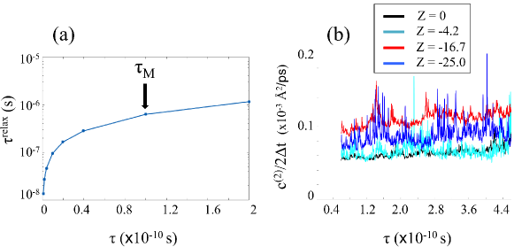
Figure S5: Evolution of (a) the slowest relaxation time, $\tau^{\textrm{relax}}$, and (b) the conditional moment $c^{(2)}$ for different values of the position $Z$ of the ligand through the POPC membrane measured for $N_{\textrm{bin}}=1000$.

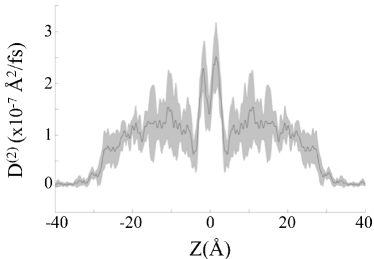
Figure S6: Diffusion profile associated with the crossing of Domperidone through the (POPC) bilayer and reconstructed along the distance from the center of the bilayer, $Z$, measured for $N_{\textrm{bin}}=1000$. Uncertainties, as represented in shaded area, were determined by dividing the data into two equal sections, determining the profiles independently, and calculating the standard error.

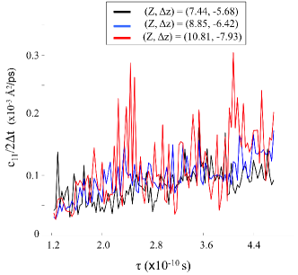
Figure S7: Evolution of the diagonal conditional moments $c_{11}^{(2)}$ obtained in the analysis of the membrane permeation in 2D for three different positions in the potential energy surface $(Z,\Delta z)$ and $N_{\textrm{bin}}=50\times 50$.

References

- Ghashghaie et al. [1996] S. Ghashghaie, W. Breymann, J. Peinke, P. Talkner, and Y. Dodge, Turbulent cascades in foreign exchange markets, Nature 381, 767 (1996).
- Naert et al. [1997] A. Naert, R. Friedrich, and J. Peinke, Fokker-planck equation for the energy cascade in turbulence, Phys. Rev. E 56, 6719 (1997).
- Lück et al. [1999] S. Lück, J. Peinke, and R. Friedrich, Uniform statistical description of the transition between near and far field turbulence in a wake flow, Phys. Rev. Lett. 83, 5495 (1999).
- Hummer [2005] G. Hummer, Position-dependent diffusion coefficients and free energies from bayesian analysis of equilibrium and replica molecular dynamics simulations, New J. Phys. 7, 34 (2005).
- Ma et al. [2006] A. Ma, A. Nag, and A. Dinner, Dynamic coupling between coordinates in a model for biomolecular isomerization, J. Chem. Phys. 124, 144911 (2006).
- Bahraminasab et al. [2009] A. Bahraminasab, F. Ghasemi, A. Stefanovska, P. McClintock, and R. Friedrich, Physics of brain dynamics: Fokker-planck analysis reveals changes in eeg interactions in anaesthesia, New J. Phys. 11, 103051 (2009).
- Best and Hummer [2010] R. Best and G. Hummer, Coordinate-dependent diffusion in protein folding, Proc. Natl. Acad. Sci. USA 107, 1088 (2010).
- Comer et al. [2013] J. Comer, C. Chipot, and F. Gonzalez-Nilo, Calculating position-dependent diffusivity in biased molecular dynamics simulations, J. Chem. Theory Comput. 9, 876 (2013).
- Lee et al. [2016] C. Lee, J. Comer, C. Herndon, N. Leung, A. Pavlova, R. Swift, C. Tung, C. Rowley, R. Amaro, C. Chipot, Y. Wang, and J. Gumbart, Simulation-based approaches for determining membrane permeability of small compounds, J. Chem. Inf. Model. 56, 721 (2016).
- Gaalswyk et al. [2016] K. Gaalswyk, E. Awoonor-Williams, and C. Rowley, Generalized langevin methods for calculating transmembrane diffusivity, J. Chem. Theory Comput. 12, 5609 (2016).
- Badaoui et al. [2018] M. Badaoui, A. Kells, C. Molteni, C. Dickson, V. Hornak, and E. Rosta, Calculating kinetic rates and membrane permeability from biased simulations, J. Phys. Chem. B 122, 11571 (2018).
- Kramers [1940] H. Kramers, Brownian motion in a field of force and the diffusion model of chemical reactions, Physica 7, 284 (1940).
- Hanggi et al. [1990] P. Hanggi, P. Talkner, and M. Borkovec, Reaction-rate theory: fifty years after kramers, Rev. Mod. Phys. 62, 251 (1990).
- Sicard [2018] F. Sicard, Computing transition rates for rare event: When kramers theory meets the free-energy landscape, Phys. Rev. E 98, 052408 (2018).
- Sicard and Senet [2013] F. Sicard and P. Senet, Reconstructing the free-energy landscape of met-enkephalin using dihedral principal component analysis and well-tempered metadynamics, J. Chem. Phys. 138, 235101 (2013).
- Sicard et al. [2015] F. Sicard, N. Destainville, and M. Manghi, Dna denaturation bubbles: Free-energy landscape and nucleation/closure rates, J. Chem. Phys. 142, 034903 (2015).
- Tiwary and van de Walle [2016] P. Tiwary and A. van de Walle, A Review of Enhanced Sampling Approaches for Accelerated Molecular Dynamics (Springer, Cham. Switzerland, 2016).
- Sicard et al. [2018] F. Sicard, T. Bui, D. Monteiro, Q. Lan, M. Ceglio, C. Burress, and A. Striolo, Emergent properties of antiagglomerant films control methane transport: Implications for hydrate management, Langmuir 34, 9701 (2018).
- Sicard et al. [2019] F. Sicard, J. Toro-Mendoza, and A. Striolo, Nanoparticles actively fragment armored droplets, ACS Nano 13, 9498 (2019).
- Camilloni and Pietrucci [2018] C. Camilloni and F. Pietrucci, Advanced simulation techniques for the thermodynamic and kinetic characterization of biological systems, Adv. Phys. X 3, 1477531 (2018).
- Sicard et al. [2020] F. Sicard, N. Destainville, P. Rousseau, C. Tardin, and M. Manghi, Dynamical control of denaturation bubble nucleation in supercoiled dna minicircles, Phys. Rev. E 101, 012403 (2020).
- Einstein [1956] A. Einstein, Investigations on the Theory of the Brownian Movement (Dover Books on Physics Series; Dover Publications, 1956).
- Kubo [1966] R. Kubo, The fluctuation-dissipation theorem, Rep. Prog. Phys. 29, 255 (1966).
- Mamonov et al. [2006] A. Mamonov, M. Kurnikova, and R. Coalson, Diffusion constant of k+ inside gramicidin a: A comparative study of four computational methods, Biophys. Chem. 124, 268 (2006).
- Marrink and Berendsen [1994] S.-J. Marrink and H. Berendsen, Simulation of water transport through a lipid membrane, J. Phys. Chem. 98, 4155 (1994).
- Marrink and Berendsen [1996] S.-J. Marrink and H. Berendsen, Permeation process of small molecules across lipid membranes studied by molecular dynamics simulations, J. Phys. Chem. 100, 16729 (1996).
- Berne et al. [1988] B. Berne, M. Borkovec, and J. Straub, Classical and modern methods in reaction rate theory, J. Phys. Chem 92, 3711 (1988).
- Woolf and Roux [1994] T. Woolf and B. Roux, Conformational flexibility of o-phosphorylcholine and o-phosphorylethanolamine: A molecular dynamics study of solvation effects, J. Am. Chem. Soc. 116, 5916 (1994).
- Türkcan et al. [2012] S. Türkcan, A. Alexandrou, and J. Masson, A bayesian inference scheme to extract diffusivity and potential fields from confined single-molecule trajectories, Biophys. J. 102, 2288 (2012).
- Rosta and Hummer [2015] E. Rosta and G. Hummer, Free energies from dynamic weighted histogram analysis using unbiased markov state model, J. Chem. Theory Comput. 11, 276 (2015).
- Risken [1966] H. Risken, The Fokker-Planck Equation (Springer, Berlin, 1966).
- Anteneodo and Riera [2009] C. Anteneodo and R. Riera, Arbitrary-order corrections for finite-time drift and diffusion coefficients, Phys. Rev. E 80, 031103 (2009).
- Petelczyc et al. [2009] M. Petelczyc, J. Zebrowski, and R. Baranowski, Kramers-moyal coefficients in the analysis and modeling of heart rate variability, Phys. Rev E 80, 031127 (2009).
- Rinn et al. [2016] P. Rinn, P. Lind, M. Wachter, and J. Peinke, The langevin approach: An r package for modeling markov processes, J. Open Research Soft. 4, e34 (2016).
- Gorjao and Meirinhos [2019] L. R. Gorjao and F. Meirinhos, Kramersmoyal: Kramers-moyal coefficients for stochastic processes, J. Open Source Soft. 4, 1693 (2019).
- Stelzl et al. [2017] L. Stelzl, A. Kells, E. Rosta, and G. Hummer, Dynamic histogram analysis to determine free energies and rates from biased simulations, J. Chem. Theory Comput. 13, 6328 (2017).
- Olsson et al. [2017] S. Olsson, H. Wu, F. Paul, C. Clementi, and F. Noé, Combining experimental and simulation data of molecular processes via augmented markov models, Proc. Natl.Acad. Sci. USA 114, 8265 (2017).
- Husic and Pande [2018] B. Husic and V. Pande, Markov state models: From an art to a science, J. Am. Chem. Soc. 140, 2386 (2018).
- Biswas et al. [2018] M. Biswas, B. Lickert, and G. Stock, Metadynamics enhanced markov modeling of protein dynamics, J. Phys. Chem. B 122, 5508 (2018).
- Farago and Grønbech-Jensen [2014a] O. Farago and N. Grønbech-Jensen, Langevin dynamics in inhomogeneous media: Re-examining the itô-stratonovich dilemma, Phys. Rev. E 89, 013301 (2014a).
- Bodrova et al. [2016] A. Bodrova, A. Chechkin, A. Cherstvy, H. Safdari, I. Sokolov, and R. Metzler, Underdamped scaled brownian motion: (non-)existence of the overdamped limit in anomalous diffusion, Sci. Rep. 6, 30520 (2016).
- Regev et al. [2016] S. Regev, N. Grønbech-Jensen, and O. Farago, Isothermal langevin dynamics in systems with power-law spatially dependent friction, Phys. Rev. E 94, 012116 (2016).
- Lau and Lubensky [2007] A. Lau and T. Lubensky, State-dependent diffusion: Thermodynamic consistency and its path integral formulation, Phys.Rev.E 76, 011123 (2007).
- G.Bussi and Parrinello [2007] G.Bussi and M. Parrinello, Accurate sampling using langevin dynamics, Phys.Rev.E 75, 056707 (2007).
- Farago and Grønbech-Jensen [2014b] O. Farago and N. Grønbech-Jensen, Fluctuation–dissipation relation for systems with spatially varying friction, J. Stat. Phys. 156, 1093–1110 (2014b).
- Friedrich and Peinke [1997] R. Friedrich and J. Peinke, Description of a turbulent cascade by a fokker-planck equation, Phys. Rev. Lett. 78, 863 (1997).
- Siegert et al. [1998] S. Siegert, R. Friedrich, and J. Peinke, Analysis of data sets of stochastic systems, Phys. Lett. A 243, 275 (1998).
- Friedrich et al. [2011] R. Friedrich, J. Peinke, M. Sahimi, and M. Tabar, Approaching complexity by stochastic methods: From biological systems to turbulence, Phys. Rep. 506, 87 (2011).
- Honisch and Friedrich [2011] C. Honisch and R. Friedrich, Estimation of kramers-moyal coefficients at low sampling rates, Phys. Rev. E 84, 019906 (2011).
- Pande et al. [2010] V. Pande, K. Beauchamp, and G. Bowman, Everything you wanted to know about markov state models but were afraid to ask, Methods 52, 99 (2010).
- Prinz et al. [2011] J.-H. Prinz, H.Wu, M. Sarich, B. Keller, M. Senne, M. Held, J. D. Chodera, C. Schütte, and F. Noé, Markov models of molecular kinetics: Generation and validation, J.Chem.Phys 134, 174105 (2011).
- Prinz et al. [2014] J.-H. Prinz, J. Chodera, and F. Noé, Estimation and Validation of Markov Models, in An Introduction to Markov State Models and Their Application to Long Timescale Molecular Simulation (Springer, New York, 2014).
- Kells et al. [2018] A. Kells, A. Annibale, and E. Rosta, Limiting relaxation times from markov state models, J. Chem. Phys. 149, 072324 (2018).
- Bowman et al. [2014] G. R. Bowman, V. S. Pande, and F. Noé, An introduction to markov state models and their application to long timescale molecular simulation, in Advances in Experimental Medicine and Biology (Springer, Dordrecht, 2014).
- Wu et al. [2016] H. Wu, F. Paul, C. Wehmeyer, and F. Noé, Multiensemble markov models of molecular thermodynamics and kinetics, Proc. Natl. Acad. Sci. USA 113, E3221 (2016).
- Donati et al. [2017] L. Donati, C. Hartmann, and B. Keller, Girsanov reweighting for path ensembles and markov state models, J. Chem. Phys. 146, 244112 (2017).
- Kieninger et al. [2020] S. Kieninger, L. Donati, and B. Keller, Dynamical reweighting methods for markov models, Curr. Opin. Struc. Bio. 61, 124 (2020).
- Medasani et al. [1998] S. Medasani, J. Kim, and R. Krishnapuram, An overview of membership function generation techniques for pattern recognition, Int. J. Approx. Reason. 19, 391 (1998).
- Kells et al. [2019] A. Kells, Z. Miháka, A. Annibale, and E. Rosta, Mean first passage times in variational coarse graining using markov state models, J. Chem. Phys. 150, 134107 (2019).
- Kells et al. [2006] A. Kells, Z. Miháka, A. Annibale, and E. Rosta, Second-order integrators for langevin equations with holonomic constraints, Chem. Phys. Lett. 429, 310 (2006).
- Freund and Poschel [2000] J. Freund and T. Poschel, Stochastic Processes in Physics, Chemistry, and Biology (Springer, Berlin, Heidelberg, 2000).
- Ren et al. [2005] W. Ren, E. Vanden-Eijnden, P. Maragakis, and E. Weinan, Transition pathways in complex systems: Application of the finite-temperature string method to the alanine dipeptide, J. Chem. Phys. 123, 134109 (2005).
- Vymetal and Vondrasek [2010] J. Vymetal and J. Vondrasek, Metadynamics as a tool for mapping the conformational and free-energy space of peptides - the alanine dipeptide case study, J. Phys. Chem. B 114, 5632–5642 (2010).
- Yonezawa et al. [2011] Y. Yonezawa, I. Fukuda, N. Kamiya, H. Shimoyama, and H. Nakamura, Free energy landscapes of alanine dipeptide in explicit water reproduced by the force-switching wolf method, J. Chem. Theory Comput. 7, 1484–1493 (2011).
- Tiwary and Parrinello [2013] P. Tiwary and M. Parrinello, From metadynamics to dynamics, Phys. Rev. Lett. 111, 230602 (2013).
- Cuny et al. [2017] J. Cuny, K. Korchagina, C. Menakbi, and T. Mineva, Metadynamics combined with auxiliary density functional and density functional tight-binding methods: alanine dipeptide as a case study, J. Mol. Model 23, 72 (2017).
- Bussi et al. [2007] G. Bussi, D. Donadio, and M. Parrinello, Canonical sampling through velocity rescaling, J. Chem. Phys. 126, 014101 (2007).
- Case et al. [2005] D. Case, T. Cheatham, T. Darden, H. Gohlke, R. Luo, K. J. Merz, A. Onufriev, C. Simmerling, B. Wang, and R. Woods, The amber biomolecular simulation programs, J. Comp. Chem. 26, 1668 (2005).
- Jorgensen et al. [1983] W. Jorgensen, J. Chandrasekhar, J. Madura, R. Impey, and M. Klein, Comparison of simple potential functions for simulating liquid water, J. Chem. Phys. 79, 926935 (1983).
- Lindahl et al. [2001] E. Lindahl, B. Hess, and D. V. D. Spoel, Gromacs 3.0: a package for molecular simulation and trajectory analysis, J. Mol. Model. 7, 306 (2001).
- Hess et al. [1997] B. Hess, H. Bekker, H. Berendsen, and J. Fraaije, Lincs: A linear constraint solver for molecular simulations, J. Comput. Chem. 98, 1463 (1997).
- Darden et al. [1993] T. Darden, D. York, and L. Pedersen, Particle mesh ewald: An nlog(n) method for ewald sums in large systems, J. Chem. Phys. 98, 10089 (1993).
- Hummer and Kevrekidis [2003] G. Hummer and I. Kevrekidis, Coarse molecular dynamics of a peptide fragment: Free energy, kinetics, and long-time dynamics computations, J. Chem. Phys. 118, 10762 (2003).
- Eyer et al. [2014] K. Eyer, F. Paech, F. Schuler, P. Kuhn, R. Kissner, S. Belli, P. Dittrich, and S. Krämer, A liposomal fluorescence assay to study permeation kinetics of drug-like weak bases across the lipid bilayer, J. Control. Release 173, 102 (2014).
- Dickson et al. [2017] C. Dickson, V. Hornak, R. Pearlstein, and J. Duca, Structure-kinetic relationships of passive membrane permeation from multiscale modeling, J. Am. Chem. Soc. 139, 442 (2017).
- Shinoda [2016] W. Shinoda, Permeability across lipid membranes, Biochim. Biophys. Acta 1858, 2254 (2016).
- Amaro and Mulholland [2018] R. Amaro and A. Mulholland, Multiscale methods in drug design bridge chemical and biological complexity in the search for cures, Nat. Rev. Chem. 2, 0148 (2018).