Generalized Rescaled Pólya urn and its statistical applications

Abstract

We introduce the Generalized Rescaled Pólya (GRP) urn, that provides a generative model for a chi-squared test of goodness of fit for the long-term probabilities of clustered data, with independence between clusters and correlation, due to a reinforcement mechanism, inside each cluster. We apply the proposed test to a data set of Twitter posts about COVID-19 pandemic: in a few words, for a classical chi-squared test the data result strongly significant for the rejection of the null hypothesis (the daily long-run sentiment rate remains constant), but, taking into account the correlation among data, the introduced test leads to a different conclusion. Beside the statistical application, we point out that the GRP urn is a simple variant of the standard Eggenberger-Pólya urn, that, with suitable choices of the parameters, shows “local” reinforcement, almost sure convergence of the empirical mean to a deterministic limit and different asymptotic behaviours of the predictive mean. Moreover, the study of this model provides the opportunity to analyze stochastic approximation dynamics, that are unusual in the related literature.
Keywords: central limit theorem, chi-squared test, Pólya urn, preferential attachment, reinforcement learning, reinforced stochastic process, stochastic approximation, urn model.

MSC2010 Classification: 60F05, 60F15, 62F03, Secondary 62F05, 62L20.

1 Introduction

The standard Eggenberger-Pólya urn (see EggPol23,mah) has been widely studied and generalized (for instance, some recent variants can be found in [7, 8, 11, 15, 18, 33, 34, 35]). In its simplest form, this model with $k$-colors works as follows. An urn contains $N_{0\,i}$ balls of color $i$, for $i=1,\dots,k$, and, at each discrete time, a ball is extracted from the urn and then it is returned inside the urn together with $\alpha>0$ additional balls of the same color. Therefore, if we denote by $N_{n\,i}$ the number of balls of color $i$ in the urn at time $n$, we have

$$N_{n\,i}=N_{n-1\,i}+\alpha\xi_{n\,i}\qquad\mbox{for }n\geq 1,$$

where $\xi_{n\,i}=1$ if the extracted ball at time $n$ is of color $i$, and $\xi_{n\,i}=0$ otherwise. The parameter $\alpha$ regulates the reinforcement mechanism: the greater $\alpha$, the greater the dependence of $N_{n\,i}$ on $\sum_{h=1}^{n}\xi_{h\,i}$.
The Generalized Rescaled Pólya (GRP) urn model is characterized by the introduction of the sequence $(\beta_{n})_{n}$ of parameters, together with the replacement of the parameter $\alpha$ of the original model by a sequence $(\alpha_{n})_{n}$, so that

$$N_{n\,i} =b_{0\,i}+B_{n\,i}$$ with

$$B_{n+1\,i} =\beta_{n}B_{n\,i}+\alpha_{n+1}\xi_{n+1\,i} n\geq 0.$$

Therefore, the urn initially contains $b_{0\,i}+B_{0\,i}$ balls of color $i$ and the parameters $\beta_{n}\geq 0$, together with $\alpha_{n}>0$, regulate the reinforcement mechanism. More precisely, the term $\beta_{n}B_{n\,i}$ links $N_{n+1\,i}$ to the “configuration” at time $n$ through the “scaling” parameter $\beta_{n}$, and the term $\alpha_{n+1}\xi_{n+1\,i}$ links $N_{n+1\,i}$ to the outcome of the extraction at time $n+1$ through the parameter $\alpha_{n+1}$.
We are going to show that, with a suitable choice of the model parameters, we have a long-term almost sure convergence of the empirical mean $\sum_{n=1}^{N}\xi_{n\,i}/N$ to the deterministic limit $p_{0\,i}=b_{0\,i}/\sum_{i=1}^{n}b_{0\,i}$, and a chi-squared goodness of fit result for the long-term probabilities $\{p_{0\,1},\dots,p_{0\,k}\}$. In particular, regarding the last point, we have that the chi-squared statistics

$$\chi^{2}=N\sum_{i=1}^{k}\frac{(\widehat{p}_{i}-p_{0\,i})^{2}}{p_{0\,i}}=\sum_{i=1}^{k}\frac{(O_{i}-Np_{0\,i})^{2}}{Np_{0\,i}},$$ (1.1)

where $N$ is the size of the sample, $\widehat{p}_{i}=O_{i}/N$, with $O_{i}=\sum_{n=1}^{N}\xi_{n\,i}$ the number of observations equal to $i$ in the sample, is asymptotically distributed as $\chi^{2}(k-1)\lambda$, with $\lambda>1$, or $\chi^{2}(k-1)N^{1-2e}\lambda$, where $\lambda>0$ may be smaller than $1$, but $e$ is always strictly smaller than $1/2$. In both cases, the presence of correlation among units mitigates the effect in (1.1) of the sample size $N$, that multiplies the chi-squared distance between the observed frequencies and the expected probabilities. This aspect is important for the statistical applications in the context of a “big sample”, when a small value of the chi-squared distance might be significant, and hence a correction related to the correlation between observations is desirable (see, for instance, [9, 12, 14, 26, 27, 31, 38, 42, 43, 45]). More precisely, in the first case, the observed value of the chi-squared distance has to be compared with the “critical” value $\chi^{2}_{1-\theta}(k-1)\lambda/N$, where $\chi^{2}_{1-\theta}(k-1)$ denotes the quantile of order $1-\theta$ of the chi-squared distribution $\chi^{2}(k-1)$. In the second case, the critical value for the chi-squared distance becomes $\chi^{2}_{1-\theta}(k-1)\lambda/N^{2e}$, where, although the constant $\lambda$ may be smaller than $1$, the effect of the sample size $N$ is mitigated by the exponent $2e<1$. In other words, for this second case, the Fisher information given by the sample does not scale with the sample size $N$, but with rate $N^{2e}$. Hence, since the long-term correlation, collecting more and more data does not provide a linear increment of the information.
Summing up, the GRP urn provides a theoretical framework for a chi-squared test of goodness of fit for the long-term probabilities of correlated data, generated according to a reinforcement mechanism. Specifically, we describe a possible application in the context of clustered data, with independence between clusters and correlation, due to a reinforcement mechanism, inside each cluster. In particular, we develop a suitable estimation technique for the fundamental model parameters. We then apply the proposed test to a data set of Twitter posts about COVID-19 pandemic. Given the null hypothesis that the daily long-run sentiment rate of the posts is the same for all the considered days (suitably spaced days in the period February 20th - April 20th 2020), performing a classical $\chi^{2}$ test, the data result strongly significant for the rejection of the null hypothesis, while, taking into account the correlation among posts sent in the same day, the proposed test leads to a different conclusion.
The sequel of the paper is so structured. In Section 2 we set up the notation and we define the GRP urn. In Section 3 we illustrate its relationships with previous models and we discuss the connections with related literature. In particular, the object of the present work gives us the opportunity to study Stochastic Approximation (SA) dynamics, which are infrequent in SA literature and so fill in some theoretical gaps. In Section 4 we provide the main result of this work, that is the almost sure convergence of the empirical means to the deterministic limits $p_{0\,i}$ and the goodness of fit result for the long-term probabilities $p_{0\,i}$, together with comments and examples. In Section 5 we describe a possible statistical application of the GRP urn and the related results: a chi-squared test of goodness of fit for the long-term probabilities of clustered data, with independence between clusters and correlation, due to a reinforcement mechanism, inside each cluster. We apply the proposed test to a data set of Twitter posts about COVID-19 pandemic. In Section 7 we state two convergence results for the empirical means, which are the basis for the proof of the main theorem. All the shown theoretical results are analytically proven. The proofs are left to Section S1 in the Supplementary Material [2], except for the proof of Theorem 7.2, which is methodologically new and emphasizes new techniques of martingale limit theory and so it is illustrated in Section 8. Finally, in the Supplementary Material we also provide some complements, some technical lemmas and some recalls about stochastic approximation theory and about stable convergence. When necessary, the references to the Supplementary Material are preceded by an “S”, so that (S$1.2$) will refer to the equation (S$1.2$) in [2].

2 The Generalized Rescaled Pólya (GRP) urn

In all the sequel, we suppose given two sequences of parameters $(\alpha_{n})_{n\geq 1}$, with $\alpha_{n}>0$ and $(\beta_{n})_{n\geq 0}$ with $\beta_{n}\geq 0$. Given a vector ${\boldsymbol{x}}=(x_{1},\ldots,x_{k})^{\top}\in\mathbb{R}^{k}$, we set $|{\boldsymbol{x}}|=\sum_{i=1}^{k}|x_{i}|$ and $\|{\boldsymbol{x}}\|^{2}={\boldsymbol{x}}^{\top}{\boldsymbol{x}}=\sum_{i=1}^{k}|x_{i}|^{2}$. Moreover we denote by ${\boldsymbol{1}}$ and ${\boldsymbol{0}}$ the vectors with all the components equal to $1$ and equal to $0$, respectively.

The urn initially contains $b_{0\,i}+B_{0\,i}>0$ distinct balls of color $i$, with $i=1,\dots,k$. We set ${\boldsymbol{b_{0}}}=(b_{0\,1},\dots,b_{0\,k})^{\top}$ and ${\boldsymbol{B_{0}}}=(B_{0\,1},\dots,B_{0\,k})^{\top}$. We assume $|{\boldsymbol{b_{0}}}|>0$ and we set ${\boldsymbol{p_{0}}}=\frac{{\boldsymbol{b_{0}}}}{|{\boldsymbol{b_{0}}}|}$. At each discrete time $(n+1)\geq 1$, a ball is drawn at random from the urn, obtaining the random vector ${\boldsymbol{\xi_{n+1}}}=(\xi_{n+1\,1},\ldots,\xi_{n+1\,k})^{\top}$ defined as

$$\xi_{n+1\,i}=\begin{cases}1&\text{when the extracted ball at time $n+1$ is of color $i$}\\ 0&\text{otherwise},\end{cases}$$

and the number of balls in the urn is so updated:

$${\boldsymbol{N_{n+1}}}={\boldsymbol{b_{0}}}+{\boldsymbol{B_{n+1}}}\qquad\text{with}\qquad{\boldsymbol{B_{n+1}}}=\beta_{n}{\boldsymbol{B_{n}}}+\alpha_{n+1}{\boldsymbol{\xi_{n+1}}}\,,$$ (2.1)

which gives (since $|{\boldsymbol{\xi_{n+1}}}|=1$)

$$|{\boldsymbol{B_{n+1}}}|=\beta_{n}|{\boldsymbol{B_{n}}}|+\alpha_{n+1}.$$

Therefore, setting $r^{*}_{n}=|{\boldsymbol{N_{n}}}|=|{\boldsymbol{b_{0}}}|+|{\boldsymbol{B_{n}}}|$, we get

$$r_{n+1}^{*}=r_{n}^{*}+(\beta_{n}-1)|{\boldsymbol{B_{n}}}|+\alpha_{n+1},$$ (2.2)

that is

$$r_{n+1}^{*}-r_{n}^{*}=|{\boldsymbol{b_{0}}}|(1-\beta_{n})-r_{n}^{*}(1-\beta_{n})+\alpha_{n+1}.$$ (2.3)

Moreover, setting $\mathcal{F}_{0}$ equal to the trivial $\sigma$-field and $\mathcal{F}_{n}=\sigma({\boldsymbol{\xi_{1}}},\dots,{\boldsymbol{\xi_{n}}})$ for $n\geq 1$, the conditional probabilities ${\boldsymbol{\psi_{n}}}=(\psi_{n\,1},\ldots,\psi_{n\,k})^{\top}$ of the extraction process, also called predictive means, are

$${\boldsymbol{\psi_{n}}}=E[{\boldsymbol{\xi_{n+1}}}|\mathcal{F}_{n}]=\frac{{\boldsymbol{N_{n}}}}{|{\boldsymbol{N_{n}}}|}=\frac{{\boldsymbol{b_{0}}}+{\boldsymbol{B_{n}}}}{r_{n}^{*}}\qquad n\geq 0.$$ (2.4)

It is obvious that we have $|{\boldsymbol{\psi_{n}}}|=1$. Moreover, when $\beta_{n}>0$ for all $n$, the probability $\psi_{n\,i}$ results increasing with the number of times we observed the value $i$, that is the random variables $\xi_{n\,i}$ are generated according to a reinforcement mechanism: the probability that the extraction of color $i$ occurs has an increasing dependence on the number of extractions of color $i$ occurred in the past (see, e.g. [41]). More precisely, we have

$${\boldsymbol{\psi_{n}}}=\frac{{\boldsymbol{b_{0}}}+{\boldsymbol{B_{0}}}\prod_{j=0}^{n-1}\beta_{j}+\sum_{h=1}^{n}\left(\alpha_{h}\prod_{j=h}^{n-1}\beta_{j}\right){\boldsymbol{\xi_{h}}}}{|{\boldsymbol{b_{0}}}|+|{\boldsymbol{B_{0}}}|\prod_{j=0}^{n-1}\beta_{j}+\sum_{h=1}^{n}\left(\alpha_{h}\prod_{j=h}^{n-1}\beta_{j}\right)}\,.$$ (2.5)

The dependence of ${\boldsymbol{\psi_{n}}}$ on ${\boldsymbol{\xi_{h}}}$ depends on the factor $f(h,n)=\alpha_{h}\prod_{j=h}^{n-1}\beta_{j}$, with $1\leq h\leq n,\,n\geq 0$. In the case of the standard Eggenberger-Pólya urn, that corresponds to $\alpha_{n}=\alpha>0$ and $\beta_{n}=1$ for all $n$, each observation ${\boldsymbol{\xi_{h}}}$ has the same “weight” $f(h,n)=\alpha$. Instead, if the factor $f(h,n)$ increases with $h$, then the main contribution is given by the most recent extractions. We refer to this phenomenon as “local” reinforcement. For instance, this is the case when $(\alpha_{n})$ is increasing and $\beta_{n}=1$ for all $n$. Another case is when $\alpha_{n}=\alpha>0$ and $\beta_{n}<1$ for all $n$. The case $\beta_{n}=0$ for all $n$ is an extreme case, for which ${\boldsymbol{\psi_{n}}}$ depends only on the last extraction ${\boldsymbol{\xi_{n}}}$ (recall that conventionally $\prod_{j=n}^{n-1}=1$). For the next examples, we will show that they exhibit a broader sense local reinforcement, in the sense that the “weight” of the observations is eventually increasing with time.
By means of (2.4), together with (2.1) and (2.2), we have

$${\boldsymbol{\psi_{n+1}}}-{\boldsymbol{\psi_{n}}}=-\frac{(1-\beta_{n})}{r_{n+1}^{*}}|{\boldsymbol{b_{0}}}|\big{(}{\boldsymbol{\psi_{n}}}-{\boldsymbol{p_{0}}}\big{)}+\frac{\alpha_{n+1}}{r_{n+1}^{*}}\big{(}{\boldsymbol{\xi_{n+1}}}-{\boldsymbol{\psi_{n}}}\big{)}.$$ (2.6)

Setting ${\boldsymbol{\theta_{n}}}={\boldsymbol{\psi_{n}}}-{\boldsymbol{p_{0}}}$ and $\Delta{\boldsymbol{M_{n+1}}}={\boldsymbol{\xi_{n+1}}}-{\boldsymbol{\psi_{n}}}={\boldsymbol{\xi_{n+1}}}-{\boldsymbol{p_{0}}}-{\boldsymbol{\theta_{n}}}$ and letting $\epsilon_{n}=|{\boldsymbol{b_{0}}}|\frac{(1-\beta_{n})}{r_{n+1}^{*}}$ and $\delta_{n}=\alpha_{n+1}/r_{n+1}^{*}$, from (2.6) we obtain

$${\boldsymbol{\psi_{n+1}}}-{\boldsymbol{\psi_{n}}}=-\epsilon_{n}({\boldsymbol{\psi_{n}}}-{\boldsymbol{p_{0}}})+\delta_{n}\Delta{\boldsymbol{M_{n+1}}}$$ (2.7)

and so

$${\boldsymbol{\theta_{n+1}}}-{\boldsymbol{\theta_{n}}}=-\epsilon_{n}{\boldsymbol{\theta_{n}}}+\delta_{n}\Delta{\boldsymbol{M_{n+1}}}\,.$$ (2.8)

Therefore, the asymptotic behaviour of $({\boldsymbol{\theta_{n}}})$ depends on the two sequences $(\epsilon_{n})_{n}$ and $(\delta_{n})_{n}$.
Finally, we observe that, setting ${\boldsymbol{\overline{\xi}_{N}}}=\sum_{n=1}^{N}{\boldsymbol{\xi_{n}}}/N$ and ${\boldsymbol{\mu_{n}}}={\boldsymbol{\overline{\xi}_{n}}}-{\boldsymbol{p_{0}}}$, we have the equality

$${\boldsymbol{\mu_{n+1}}}-{\boldsymbol{\mu_{n}}}=-\frac{1}{n}({\boldsymbol{\mu_{n}}}-{\boldsymbol{\theta_{n}}})+\frac{1}{n}\Delta{\boldsymbol{M_{n+1}}},$$ (2.9)

that links the asymptotic behaviour of $({\boldsymbol{\mu_{n}}})$ and the one of $({\boldsymbol{\theta_{n}}})$.
Different kinds of sequences $(\epsilon_{n})_{n}$ and $(\delta_{n})_{n}$ provide different kinds of asymptotic behaviour of ${\boldsymbol{\theta_{n}}}$, i.e. of the empirical mean ${\boldsymbol{\overline{\xi}_{N}}}$. In Section 4, we provide two cases in which we have a long-term almost sure convergence of the empirical mean $O_{i}/N=\sum_{n=1}^{N}\xi_{n\,i}/N$ toward the constant $p_{0i}=b_{0\,i}/|{\boldsymbol{b_{0}}}|$, together with a chi-squared goodness of fit result. In particular, the quantities $p_{0\,1},\ldots,p_{0\,k}$ can be seen as a long-run probability distribution on the possible values (colors) $\{1,\dots,k\}$.

3 Related literature

The particular case when in the GRP urn model we have $\beta_{n}=\beta=0$ for all $n$ corresponds to a version of the so-called “memory-1 senile reinforced random walk” on a star-shaped graph introduced in [29]. The case $\alpha_{n}=\alpha>0$ and $\beta_{n}=\beta=1$ for all $n$ corresponds to the standard Eggenberger-Pólya urn with an initial number $N_{0\,i}=b_{0\,i}+B_{0\,i}$ of balls of color $i$. When $(\alpha_{n})$ is a not-constant sequence, while $\beta_{n}=\beta=1$ for all $n$, the GRP urn coincides with the variant of the Eggenberger-Pólya urn introduced in [40] (see also [41, Sec. 3.2]). Instead, when $\beta\neq 1$, the GRP urn does not fall in any variants of the Eggenberger-Pólya urn discussed in [41, Sec. 3.2].
The case when $\alpha_{n}=\alpha>0$ and $\beta_{n}=\beta\geq 0$ for all $n$ corresponds to the Rescaled Pólya (RP) urn introduced and studied in [1] and applied in [6]. It is worthwhile to point out that the two cases studied in the present work do not include (and are not included in) the case studied in [1]. Moreover, the techniques employed here and in [1] are completely different: when $\beta_{n}=\beta\in[0,1)$ as in [1], the jumps $\Delta{\boldsymbol{\psi_{n}}}$ do not vanish and the process ${\boldsymbol{\psi}}=({\boldsymbol{\psi_{n}}})_{n}$ converges to a stationary Markov chain and so the appropriate Markov ergodic theory is employed; in this work, we have $|\Delta{\boldsymbol{\psi_{n}}}|=o(1)$, so that the martingale limit theory is here exploited to achieve the asymptotic results. Obviously, the two techniques are not exchangeable or adaptable from one contest to the other one.
When $(\beta_{n})$ is not identically equal to $1$, since the first term in the right hand of the above relation, the GRP urn does not belong to the class of Reinforced Stochastic Processes (RSPs) studied in [3, 5, 4, 20, 21, 23]. Indeed, the RSPs are characterized by a “strict” reinforcement mechanism such that $\xi_{n\,i}=1$ implies $\psi_{n\,i}>\psi_{n-1\,i}$ and so, as a consequence, $\psi_{n\,i}$ has an increasing dependence on the number of times we have $\xi_{h\,i}=1$ for $h=1,\dots,n$. When $(\beta_{n})$ is not identically equal to $1$, the GRP urn does not satisfy the “strict” reinforcement mechanism, because the first term is positive or negative according to the sign of $(1-\beta_{n})$ and of $({\boldsymbol{\psi_{n}}}-{\boldsymbol{p_{0}}})$. Furthermore, we observe that equation (2.6) recalls the dynamics of a RSP with a “forcing input” (see [3, 20, 44]), but the main difference relies on the fact that such a process is driven by a classical stochastic approximation dynamics, that is a dynamics of the kind (2.7) with $\epsilon_{n}=\delta_{n}$ (up to a constant) with $\sum_{n}\epsilon_{n}=+\infty$ and $\sum_{n}\epsilon_{n}^{2}<+\infty$, while the GRP urn model also allows for $\epsilon_{n}$ and $\delta_{n}$ with different rates and also for

• $\sum_{n}\epsilon_{n}=+\infty$ and $\sum_{n}\delta_{n}^{2}=+\infty$ or

• $\sum_{n}\epsilon_{n}<+\infty$.

Since (2.7) is the fundamental equation of the Stochastic Approximation (SA) theory, we deem it appropriate to say a few more words on the relationship of the present work with the SA literature. The case when $\delta_{n}=c\epsilon_{n}$ in (2.7) is essentially covered by the Stochastic Approximation (SA) theory (see Section S5, where we refer to [25, 32, 37, 39, 48]). The most known case is when $\sum_{n}\epsilon_{n}=+\infty$ and $\sum_{n}\epsilon_{n}^{2}<+\infty$. The case $\epsilon_{n}\to 0$, $\sum_{n}\epsilon_{n}=+\infty$ and $\sum_{n}\epsilon_{n}^{2}=+\infty$ is less usual in literature, but it is well characterized in [32]. The case when $(\epsilon_{n})_{n}$ and $(\delta_{n})_{n}$ in (2.7) go to zero with different rates is typically neglected in SA literature. To our best knowledge, it is taken into consideration only in [39], where the weak convergence rate of the sequence $({\boldsymbol{\psi_{N}}})$ toward a certain point ${\boldsymbol{\psi^{*}}}$ is established under suitable assumptions, given the event $\{{\boldsymbol{\psi_{N}}}\to{\boldsymbol{\psi^{*}}}\}$. No result is given for the empirical mean ${\boldsymbol{\overline{\xi}}}_{N}$, which instead is the focus of the present paper (see Theorem 4.1 below, whose proof is based on Theorem 7.2). More precisely, the assumptions on $\epsilon_{n}$ and $\delta_{n}$ in the following Theorem 7.2 imply assumption (A1.3) in [39] and so Theorem 1 in that paper provides the weak convergence rate of the sequence $({\boldsymbol{\psi_{N}}}-{\boldsymbol{\psi^{*}}})$ given the event $\{{\boldsymbol{\psi_{N}}}\to{\boldsymbol{\psi^{*}}}\}$. However, this result is not useful for our scope because of two reasons: first, we need convergence results for the empirical mean ${\boldsymbol{\overline{\xi}_{N}}}$, not for the predictive mean ${\boldsymbol{\psi_{N}}}$; second, in one case included in Theorem 7.2 (see Section 7 for more details), it seems to us not immediate to check the convergence of the predictive means and so we develop another technique that does not ask for this convergence (see Section 8). Hence, the contribution of Theorem 7.2 to the SA literature is that, for a dynamics of the type (2.7) with $(\epsilon_{n})_{n}$ and $(\delta_{n})_{n}$ going to zero with different rates, it provides the asymptotic behaviour of the empirical mean ${\boldsymbol{\overline{\xi}_{N}}}$, covering a case when $\sum_{n}\epsilon_{n}=+\infty$ and $\sum_{n}\delta_{n}^{2}=+\infty$ and without requiring the convergence of the empirical means ${\boldsymbol{\psi_{N}}}$.
Finally, it is worthwhile to point out that we also analyze the case when $\sum_{n}\epsilon_{n}<+\infty$, which is also excluded in SA literature and so it could be relevant in that field. Specifically, we prove almost sure convergence of the predictive means and of the empirical means toward a random variable and we give a central limit theorem in the sense of stable convergence. However, even if interesting from a theoretical point of view, we collect these results in Section S2, because they are not related to the chi-squared test of goodness of fit.
The following statistical application of the GRP urn was inspired by [1, 12, 36]. However, those papers only deal with the case when the statistics (1.1) is asymptotically distributed as $\chi^{2}(k-1)\lambda$, with $\lambda>1$, while we also face the case when the statistics (1.1) is asymptotically distributed as $\chi^{2}(k-1)N^{1-2e}\lambda$, illustrating a suitable estimation procedure for the fundamental parameters $\eta=1-2e$ and $\lambda$. To the best of our knowledge, this is the first work presenting a model that provides a theoretical framework for a such chi-squared test of goodness of fit.

4 Main theorem: goodness of fit result

Given a sample $({\boldsymbol{\xi_{1}}},\ldots,{\boldsymbol{\xi_{N}}})$ generated by a GRP urn, the statistics

$$O_{i}=\#\{n=1,\dots,N\colon\xi_{n\,i}=1\}=\sum_{n=1}^{N}\xi_{n\,i},\,\qquad i=1,\ldots,k,$$

counts the number of times we observed the value $i$. The theorem below states, under suitable assumptions, the almost sure convergence of the empirical mean $\widehat{p}_{i}=O_{i}/N=\sum_{n=1}^{N}\xi_{n\,i}/N$ toward the probability $p_{0\,i}$, together with a chi-squared goodness of fit test for the long-term probabilities $p_{0\,1},\dots,p_{0\,k}$. More precisely, we prove the following result:

Theorem 4.1.

Assume $p_{0\,i}>0$ for all $i=1,\dots,k$ and suppose to be in one of the following cases:

• $\epsilon_{n}=(n+1)^{-\epsilon}$ and $\delta_{n}=c\epsilon_{n}$, with $\epsilon\in(0,1]$ and $c>0$, or

• $\epsilon_{n}=(n+1)^{-\epsilon}$, $\delta_{n}\sim c(n+1)^{-\delta}$, with $\epsilon\in(0,1)$, $\delta\in(\epsilon/2,\epsilon)$ and $c>0$.

Define the constants $e$ and $\lambda$ as

$$e=\begin{cases}1/2\quad&\mbox{in case a) }\\ 1/2-(\epsilon-\delta)<1/2\quad&\mbox{in case b)}\end{cases}$$

and

$$\lambda=\begin{cases}(c+1)^{2}\quad&\mbox{in case a) with }\epsilon\in(0,1)\,,\\ (c+1)^{2}+c^{2}=[2c(c+1)+1]\quad&\mbox{in case a) with }\epsilon=1\,,\\ \frac{c^{2}}{1+2(\epsilon-\delta)}\quad&\mbox{in case b)}\,.\end{cases}$$ (4.1)

Then $\widehat{p}_{i}=O_{i}/N\stackrel{{\scriptstyle a.s.}}{{\longrightarrow}}p_{0\,i}$ and

$$\frac{1}{N^{1-2e}}\sum_{i=1}^{k}\frac{(O_{i}-Np_{0\,i})^{2}}{Np_{0\,i}}=N^{2e}\sum_{i=1}^{k}\frac{(\widehat{p}_{i}-p_{0\,i})^{2}}{p_{0\,i}}\mathop{\longrightarrow}^{d}_{N\to\infty}W_{*}=\lambda W_{0}$$

where $W_{0}$ has distribution $\chi^{2}(k-1)=\Gamma\big{(}\frac{k-1}{2},\frac{1}{2})$ and, consequently, $W_{*}$ has distribution $\Gamma\big{(}\frac{k-1}{2},\frac{1}{2\lambda}\big{)}$.

We note that $\lambda$ is a constant greater than $1$ in case a); while, in case b), it is a strictly positive quantity. Moreover, in case b), we have $0<(\epsilon-\delta)<\epsilon/2<1/2$ and so $(1-2e)=2(\epsilon-\delta)\in(0,1)$. As a consequence, we have $N^{1-2e}\lambda>1$ for $N$ large enough.

In the next two examples we show that it is possible to construct suitable sequences $(\alpha_{n})_{n}$ and $(\beta_{n})_{n}$ of the model such that the corresponding sequences $(\epsilon_{n})_{n}$ and $(\delta_{n})$ converge to zero with the same rate or with different rates and satisfy the assumptions a) or b) of the above theorem, respectively.

Example 4.2.

(Case $\epsilon_{n}=(n+1)^{-\epsilon}$ and $\delta_{n}=c\epsilon_{n}$, with $\epsilon>0$ and $c>0$ )
Take $\alpha_{n+1}=c|{\boldsymbol{b_{0}}}|(1-\beta_{n})$, with $\beta_{n}\in[0,1)$ and $c>0$, that implies $\delta_{n}=\frac{\alpha_{n+1}}{r_{n+1}^{*}}=c\frac{|{\boldsymbol{b_{0}}}|(1-\beta_{n})}{r_{n+1}^{*}}=c\epsilon_{n}$. Set $r^{*}_{n}=(1+c)|{\boldsymbol{b_{0}}}|(1-t_{n})$ so that from (2.3) we obtain $t_{n+1}=\beta_{n}t_{n}$. Hence, we have

$$t_{n+1}=t_{0}\prod_{k=0}^{n}\beta_{k}=\frac{c|{\boldsymbol{b_{0}}}|-|{\boldsymbol{B_{0}}}|}{(1+c)|{\boldsymbol{b_{0}}}|}\prod_{k=0}^{n}\beta_{k}$$

and so

$$r^{*}_{n+1}=(1+c)|{\boldsymbol{b_{0}}}|+\big{(}|{\boldsymbol{B_{0}}}|-c|{\boldsymbol{b_{0}}}|\big{)}\prod_{k=0}^{n}\beta_{k}.$$

Therefore, setting $\beta^{*}=\prod_{k=0}^{\infty}\beta_{k}\in[0,1)$, we get $r^{*}_{n}\longrightarrow r^{*}=(1+c)|{\boldsymbol{b_{0}}}|+(|{\boldsymbol{B_{0}}}|-c|{\boldsymbol{b_{0}}}|)\beta^{*}>0$. If we choose $|{\boldsymbol{B_{0}}}|=c|{\boldsymbol{b_{0}}}|$, then $r_{n}^{*}=r^{*}=(1+c)|{\boldsymbol{b_{0}}}|$ for each $n$ and so, setting $\beta_{n}=1-(1+c)(1+n)^{-\epsilon}$ with $\epsilon>0$, we obtain $\epsilon_{n}=(1+n)^{-\epsilon}$ and $\delta_{n}=c\epsilon_{n}$. Taking $\epsilon\in(0,1]$, we have that $\epsilon_{n}$ and $\delta_{n}$ satisfy assumption a) of Theorem 4.1. Moreover, we have $\alpha_{n}=c|{\boldsymbol{b_{0}}}|(1+c)n^{-\epsilon}$ and $1-\beta_{n}=(1+c)(1+n)^{-\epsilon}$ and so, for the behaviour of the factor $f(h,n)=\alpha_{h}\prod_{j=h}^{n-1}\beta_{j}$ in (2.5), we refer to Section S3.

Example 4.3.

(Case $\epsilon_{n}=(n+1)^{-\epsilon}$ and $\delta_{n}\sim c(n+1)^{-\delta}$, with $0<\delta<\epsilon<1$ and $c>0$)
Take $0<\delta<\epsilon<1$ and set $\gamma=\epsilon-\delta>0$, $r_{n}^{*}=n^{\gamma}$ and $(1-\beta_{n})=|{\boldsymbol{b_{0}}}|^{-1}(1+n)^{-\delta}$. We immediately have

$$\epsilon_{n}=|{\boldsymbol{b_{0}}}|\frac{(1-\beta_{n})}{r_{n+1}^{*}}=(1+n)^{-\delta-\gamma}=(n+1)^{-\epsilon}$$

and (2.3) yields $\alpha_{n+1}=(n+1)^{\gamma}-n^{\gamma}[1-|{\boldsymbol{b_{0}}}|^{-1}(1+n)^{-\delta}]-(1+n)^{-\delta}$, so that

$$\begin{split}\delta_{n}&=\frac{\alpha_{n+1}}{r_{n+1}^{*}}=\frac{\alpha_{n+1}}{(n+1)^{\gamma}}=1-\Big{(}1-\frac{1}{n+1}\Big{)}^{\gamma}\big{[}1-|{\boldsymbol{b_{0}}}|^{-1}(1+n)^{-\delta}\big{]}-(1+n)^{-\delta-\gamma}\\ &=1-\Big{(}1-\gamma(n+1)^{-1}+O(n^{-2})\Big{)}\big{[}1-|{\boldsymbol{b_{0}}}|^{-1}(1+n)^{-\delta}\big{]}-(1+n)^{-\epsilon}\\ &=|{\boldsymbol{b_{0}}}|^{-1}(1+n)^{-\delta}\Big{(}1+\gamma|{\boldsymbol{b_{0}}}|(n+1)^{-1+\delta}-|{\boldsymbol{b_{0}}}|(1+n)^{-\epsilon+\delta}-\gamma(n+1)^{-1}+O(n^{-2+\delta})\Big{)}\,.\end{split}$$

Setting $c=|{\boldsymbol{b_{0}}}|^{-1}>0$, we obtain $\epsilon_{n}=(n+1)^{-\epsilon}$ and $\delta_{n}\sim c(n+1)^{-\delta}$. Taking $\delta\in(\epsilon/2,\epsilon)$, we have that $\epsilon_{n}$ and $\delta_{n}$ satisfy assumption b) of Theorem 4.1. Moreover, we have $\alpha_{n}=cn^{-(2\delta-\epsilon)}(1+\gamma c^{-1}n^{-1+\delta}-c^{-1}n^{-\epsilon+\delta}-\gamma n^{-1}+O(n^{-2+\delta}))$ and $(1-\beta_{n})=c(1+n)^{-\delta}$, with $0<2\delta-\epsilon<\delta<(1+2\delta-\epsilon)/2$, and so, for the behaviour of the factor $f(h,n)=\alpha_{h}\prod_{j=h}^{n-1}\beta_{j}$ in (2.5), we refer to Section S3.

5 Statistical applications

In a big sample the units typically can not be assumed independent and identically distributed, but they exhibit a structure in clusters, with independence between clusters and with correlation inside each cluster [12, 17, 30, 36, 46, 47]. The model and the related results presented in [1] and in the present paper may be useful in the situation when inside each cluster the probability that a certain unit chooses the value $i$ is affected by the number of units in the same cluster that have already chosen the value $i$, hence according to a reinforcement rule. Formally, given a “big” sample $\{{\boldsymbol{\xi}}_{n}:\,n=1,\dots,N\}$, we suppose that the $N$ units are ordered so that we have the following $L$ clusters of units:

$$C_{\ell}=\left\{\sum_{l=1}^{\ell-1}N_{l}+1,\dots,\sum_{l=1}^{\ell}N_{l}\right\},\qquad\ell=1,\dots,L.$$

Therefore, the cardinality of each cluster $C_{\ell}$ is $N_{\ell}$. We assume that the units in different clusters are independent, that is

$$[{\boldsymbol{\xi_{1}}},\dots,{\boldsymbol{\xi_{N_{1}}}}],\,\dots\,,[{\boldsymbol{\xi_{\sum_{l=1}^{\ell-1}N_{l}+1}}},\dots,{\boldsymbol{\xi_{\sum_{l=1}^{\ell}N_{l}}}}],\,\dots\,,[{\boldsymbol{\xi_{\sum_{l=1}^{L-1}N_{l}+1}}},\dots,{\boldsymbol{\xi_{N}}}]$$

are $L$ independent multidimensional random variables. Moreover, we assume that the observations inside each cluster can be modelled as a GRP satisfying case a) or case b) of Theorem 4.1. Given certain (strictly positive) intrinsic probabilities $p_{0\,1}^{*}(\ell),\dots,p_{0\,k}^{*}(\ell)$ for each cluster $C_{\ell}$, we firstly want to estimate the model parameters and then perform a test with null hypothesis

$$H_{0}:\quad p_{0\,i}(\ell)=p_{0\,i}^{*}(\ell)\quad\forall i=1,\dots,k$$

based on the the statistics

$$Q_{\ell}=\frac{1}{N_{\ell}^{2(\epsilon-\delta)}}\sum_{i=1}^{k}\frac{\big{(}O_{i}(\ell)-N_{\ell}p_{0\,i}^{*}(\ell)\big{)}^{2}}{N_{\ell}p_{0\,i}^{*}(\ell)},\quad\mbox{with}\;O_{i}(\ell)=\#\{n\in C_{\ell}:\,\xi_{n\,i}=1\},$$ (5.1)

and its corresponding asymptotic distribution $\Gamma\big{(}\frac{k-1}{2},\frac{1}{2\lambda}\big{)}$, where $\lambda$ is given in (4.1). Note that we can perform the above test for a certain cluster $\ell$, or we can consider all the clusters together using the aggregate statistics $\sum_{\ell=1}^{L}Q_{\ell}$ and its corresponding distribution $\Gamma(\frac{L(k-1)}{2},\frac{1}{2\lambda})$.
Regarding the probabilities $p_{0\,i}^{*}(\ell)$, some possibilities are:

• we can take $p_{0\,i}^{*}(\ell)=1/k$ for all $i=1,\dots,k$ if we want to test possible differences in the probabilities for the $k$ different values;

• we can suppose to have two different periods of times, and so two samples, say $\{{\boldsymbol{\xi^{(1)}_{n}}}:\,n=1,\dots,N\}$ and $\{{\boldsymbol{\xi^{(2)}_{n}}}:\,n=1,\dots,N\}$, take $p_{0\,i}^{*}(\ell)=\sum_{n\in C_{\ell}}\xi^{(1)}_{n\,i}/N_{\ell}$ for all $i=1,\dots,k$, and perform the test on the second sample in order to check possible changes in the intrinsic long-run probabilities;

• we can take one of the clusters as benchmark, say $\ell^{*}$, set $p_{0\,i}^{*}(\ell)=\sum_{n\in C_{\ell^{*}}}\xi_{n\,i}/N_{\ell^{*}}$ for all $i=1,\dots,k$ and $\ell\neq\ell^{*}$, and perform the test for the other $L-1$ clusters in order to check differences with the benchmark cluster $\ell^{*}$.

Finally, if we want to test possible differences in the clusters, then we can take $p_{0\,i}^{*}(\ell)=p_{0\,i}^{*}=\sum_{n=1}^{N}\xi_{n\,i}/N$ for all $\ell=1,\dots,L$ and perform the test using the aggregate statistics $\sum_{\ell=1}^{L}Q_{\ell}$ with asymptotic distribution $\Gamma(\frac{(L-1)(k-1)}{2},\frac{1}{2\lambda})$.

5.1 Estimation of the parameters

The model parameters are $\epsilon,\delta$ and $c$. However, as we have seen, the fundamental quantities are $\eta=2(\epsilon-\delta)$ and $\lambda$ given in (4.1). Moreover, recall that in case a), we have $\eta=0$ and $\lambda>1$ and, in case b), we have $\eta\in(0,1)$ and $\lambda>0$. Therefore, according the considered model, the pair $(\eta,\,\lambda)$ belongs to $S=\{0\}\times(1,+\infty)\cup(0,1)\times(0,+\infty)$. In order to estimate the pair $(\eta,\lambda)\in S$, we define

$$T_{\ell}=N_{\ell}^{\eta}Q_{\ell}=\sum_{i=1}^{k}\frac{\big{(}O_{i}(\ell)-N_{\ell}p_{0\,i}^{*}(\ell)\big{)}^{2}}{N_{\ell}p_{0\,i}^{*}(\ell)}\,.$$

Given the observed values $t_{1},\dots,t_{L}$, the log-likelihood function of $Q_{\ell}$ reads

$$\ln(\mathcal{L}(\eta,\,\lambda))=\ln\mathcal{L}(\eta,\,\lambda;\,t_{1},\dots,t_{L})=-\frac{k-1}{2}L\ln(\lambda)-\frac{k-1}{2}\eta\sum_{\ell=1}^{L}\ln(N_{\ell})-\tfrac{1}{2\lambda}\sum_{\ell=1}^{L}{\tfrac{t_{\ell}}{N_{\ell}^{\eta}}}+R_{1}\,,$$

where $R_{1}$ is a remainder term that does not depend on $(\eta,\,\lambda)$. Now, we look for the maximum likelihood estimator of the two parameters $(\eta,\,\lambda)$.
We immediately observe that, when all the clusters have the same cardinality, that is all the $N_{\ell}$ are equal to a certain $N_{0}$, then we cannot hope to estimate $\eta$ and $\lambda$, separately. Indeed, the log-likelihood function becomes

$$\ln(\mathcal{L}(\eta,\,\lambda))=\ln\mathcal{L}(\eta,\,\lambda;\,t_{1},\dots,t_{L})=-\frac{k-1}{2}L\Big{[}\ln(\lambda)+\eta\ln(N_{0})\Big{]}-\tfrac{1}{2\lambda N_{0}^{\eta}}\sum_{\ell=1}^{L}t_{\ell}+R_{1}=f(\lambda N_{0}^{\eta})\,.$$

This fact implies that it possible to estimate only the parameter $(\lambda N_{0}^{\eta})$ as $\widehat{\lambda N_{0}^{\eta}}=\sum_{\ell=1}^{L}t_{\ell}/(k-1)L$.
From now on, we assume that at least two clusters have different cardinality, that is at least a pair of cardinalities $N_{\ell}$ are different. We have to find (if they exist!) the maximum points of the function $(\eta,\,\lambda)\mapsto\ln(\mathcal{L}(\eta,\,\lambda))$ on the set $S$, which is not closed nor limited. First of all, we note that $\ln(\mathcal{L}(\eta,\,\lambda))\to-\infty$ for $\lambda\to+\infty$ and $\lambda\to 0$. Thus, the log-likelihood function has maximum value on the closure $\overline{S}$ of $S$ and its maximum points are stationary points belonging to $(0,1)\times(0,+\infty)$ or they belong to $\{0,1\}\times(0,+\infty)$. For detecting the points of the first type, we compute the gradient of the log-likelihood function, obtaining

$$\nabla_{(\eta,\,\lambda)}\ln\mathcal{L}=\begin{pmatrix}-\frac{k-1}{2}\sum_{\ell=1}^{L}\ln(N_{\ell})+\tfrac{1}{2\lambda}\sum_{\ell=1}^{L}{\tfrac{t_{\ell}\ln(N_{\ell})}{N_{\ell}^{\eta}}}\\ -\frac{k-1}{2\lambda}L+\tfrac{1}{2\lambda^{2}}\sum_{\ell=1}^{L}{\tfrac{t_{\ell}}{N_{\ell}^{\eta}}}\end{pmatrix}\,.$$

Hence, the stationary points $(\eta,\,\lambda)$ of the log-likelihood function are solutions of the system

$$\left\{\begin{aligned} &\frac{\sum_{\ell=1}^{L}\tfrac{t_{\ell}}{N_{\ell}^{\eta}}\ln(N_{\ell})}{\sum_{\ell=1}^{L}\tfrac{t_{\ell}}{N_{\ell}^{\eta}}}=\frac{\sum_{\ell=1}^{L}\ln(N_{\ell})}{L}\\ &\lambda=\frac{\sum_{\ell=1}^{L}\tfrac{t_{\ell}}{N_{\ell}^{\eta}}}{L(k-1)}\,.\end{aligned}\right.$$

In particular, we get that the stationary points are of the form $(\eta,\,\lambda(\eta))$, with

$$\lambda(\eta)=\frac{\sum_{\ell=1}^{L}\tfrac{t_{\ell}}{N_{\ell}^{\eta}}}{L(k-1)}\,.$$ (5.2)

In order to find the maximum points on the border, that is belonging to $\{0,1\}\times(0,+\infty)$, we observe that, fixed any $\eta$, the function

$$\lambda\mapsto-\frac{k-1}{2}L\ln(\lambda)-\tfrac{1}{2\lambda}\sum_{\ell=1}^{L}{\tfrac{t_{\ell}}{N_{\ell}^{\eta}}}+R_{2}\,,$$

where $R_{2}$ is a remainder term not depending on $\lambda$, takes its maximum value at the point $\lambda(\eta)$ defined in (5.2).
Summing up, the problem of detecting the maximum points of the log-likelihood function on $\overline{S}$ reduces to the study of the maximum points on $[0,1]$ of the function

$$\eta\mapsto\ln(\mathcal{L}(\eta,\,\lambda(\eta)))=-\frac{k-1}{2}L\ln\Big{(}\sum_{\ell=1}^{L}{\frac{t_{\ell}}{N_{\ell}^{\eta}}}\Big{)}-\frac{k-1}{2}\eta\sum_{\ell=1}^{L}\ln(N_{\ell})+R_{3}\,,$$ (5.3)

where $R_{3}$ is a remainder term not depending on $\eta$. To this purpose, we note that we have

$$d\frac{\ln(\mathcal{L}(\eta,\,\lambda(\eta))}{d\eta}=\frac{k-1}{2}L\left[\frac{\sum_{\ell=1}^{L}{\tfrac{t_{\ell}}{N_{\ell}^{\eta}}}\ln(N_{\ell})}{\sum_{\ell=1}^{L}{\frac{t_{\ell}}{N_{\ell}^{\eta}}}}-\frac{\sum_{\ell=1}^{L}\ln(N_{\ell})}{L}\right]=\frac{(k-1)L}{2}g(\eta)\,,$$

where

$$g(x)=\frac{\sum_{\ell=1}^{L}{\tfrac{t_{\ell}}{N_{\ell}^{x}}}\ln(N_{\ell})}{\sum_{\ell=1}^{L}{\tfrac{t_{\ell}}{N_{\ell}^{x}}}}-\frac{\sum_{\ell=1}^{L}\ln(N_{\ell})}{L}\,.$$

Setting

$$p(x,\ell)=\frac{\tfrac{t_{\ell}}{N_{\ell}^{x}}}{\sum_{l=1}^{L}\tfrac{t_{l}}{N_{l}^{x}}}$$

and denoting by $\mathop{E_{x}}[\cdot]$ and by $E_{u}[\cdot]$ the mean value with respect to the discrete probability distribution $\{p(x,\ell):\,\ell=1,\dots,L\}$ on $\{N_{1},\dots,N_{L}\}$ and with respect to the uniform discrete distribution on $\{N_{1},\dots,N_{L}\}$ respectively, the above function $g$ can be written as

$$g(x)=\sum_{\ell=1}^{L}p(x,\ell)\ln(N_{\ell})-\frac{\sum_{\ell=1}^{L}\ln(N_{\ell})}{L}=\mathop{E_{x}}[\ln(N)]-\mathop{E_{u}}[\ln(N)]\,.$$

Moreover, we have

$$\begin{split}g^{\prime}(x)&=\frac{\Big{(}-\sum_{\ell=1}^{L}{\tfrac{t_{\ell}}{N_{\ell}^{x}}}\ln^{2}(N_{\ell})\Big{)}\Big{(}\sum_{\ell=1}^{L}{\tfrac{t_{\ell}}{N_{\ell}^{x}}}\Big{)}+\Big{(}\sum_{\ell=1}^{L}{\tfrac{t_{\ell}}{N_{\ell}^{x}}}\ln(N_{\ell})\Big{)}^{2}}{\Big{(}\sum_{\ell=1}^{L}{\tfrac{t_{\ell}}{N_{\ell}^{x}}}\Big{)}^{2}}\\ &=-\sum_{\ell=1}^{L}p({x},\ell)\ln^{2}(N_{\ell})+\Big{(}\sum_{\ell=1}^{L}p({x},\ell)\ln(N_{\ell})\Big{)}^{2}=-\mathop{Var_{x}}[\ln(N)]\,,\end{split}$$

where $Var_{x}[\cdot]$ denotes the variance with respect to the discrete probability distribution $\{p(x,\ell):\,\ell=1,\dots,L\}$ on $\{N_{1},\dots,N_{L}\}$. Since, we are assuming that at least two $N_{\ell}$ are different, we have $\mathop{Var_{x}}[\ln(N)]>0$ and so the function $g$ is strictly decreasing. Finally, we observe that we have

$$\mathop{Cov_{u}}(\ln(N),T)=\frac{\sum_{\ell=1}^{L}t_{\ell}\ln(N_{\ell})}{L}-\frac{\sum_{\ell=1}^{L}t_{\ell}}{L}\frac{\sum_{\ell=1}^{L}\ln(N_{\ell})}{L}=g(0)\frac{\sum_{\ell=1}^{L}t_{\ell}}{L}$$

and

$$\mathop{Cov_{u}}(\ln(N),\tfrac{T}{N})=\frac{\sum_{\ell=1}^{L}\tfrac{t_{\ell}}{N_{\ell}}\ln(N_{\ell})}{L}-\frac{\sum_{\ell=1}^{L}\tfrac{t_{\ell}}{N_{\ell}}}{L}\frac{\sum_{\ell=1}^{L}\ln(N_{\ell})}{L}=g(1)\frac{\sum_{\ell=1}^{L}\tfrac{t_{\ell}}{N_{\ell}}}{L}\,,$$

where $Cov_{u}(\cdot,\cdot)$ denotes the covariance with respect to the discrete joint distribution concentrated on the diagonal and such that $P\{N=N_{\ell},\,T=t_{\ell}\}=1/L$ with $\ell=1,\dots,L$. Hence, we distinguish the following cases.

First case: $\mathop{Cov_{u}}(\ln(N),T)\leq 0$

We are in the case when $g(0)\leq 0$ and so the function (5.3) is strictly decreasing for $\eta>0$. Thus, its maximum value on $[0,1]$ is assumed at $\widehat{\eta}=0$. Consequently, we have $\widehat{\lambda}=\lambda(0)=\frac{\sum_{\ell=1}^{L}t_{\ell}}{L(k-1)}$. Recall that we need $(0,\widehat{\lambda})\in S$ and so $\widehat{\lambda}>1$. If the model fits well the data, this is a consequence. Indeed, $\widehat{\lambda}$ is an unbiased estimator: $\widehat{\lambda}\stackrel{{\scriptstyle d}}{{\sim}}\Gamma(L(k-1)/2,1/(2\lambda))$ and so $E[\widehat{\lambda}]=\lambda>1$. A value $\widehat{\lambda}\leq 1$ means a bad fit of the consider model to the data (the smaller the value of $\lambda$, the worse the fitting). Note that in the threshold case $(\widehat{\eta}=0,\,\widehat{\lambda}=1)$, the corresponding test statistics (5.1) and its distribution coincide with the classical ones used for independent observations.

Second case: $\mathop{Cov_{u}}(\ln(N),T)>0$ and $\mathop{Cov_{u}}(\ln(N),\tfrac{T}{N})<0$

We are in the case when $g(0)>0$ and $g(1)<0$. Hence, the function (5.3) has a unique stationary point $\widehat{\eta}\in(0,1)$, which is the maximum point. Consequently, we have $\widehat{\lambda}=\lambda(\widehat{\eta})=\frac{\sum_{\ell=1}^{L}\tfrac{t_{\ell}}{N_{\ell}^{\widehat{\eta}}}}{L(k-1)}>0$. The point $(\widehat{\eta},\widehat{\lambda})$ belongs to $S$.

Third case: $\mathop{Cov_{u}}(\ln(N),\tfrac{T}{N})\geq 0$

We are in the case when $g(1)\geq 0$ and so the function (5.3) is strictly increasing on $[0,1]$. Hence, its maximum point is at $\widehat{\eta}=1$, and, accordingly, we have $\widehat{\lambda}=\lambda(1)=\frac{\sum_{\ell=1}^{L}\tfrac{t_{\ell}}{N_{\ell}}}{L(k-1)}$. However, the point $(1,\widehat{\lambda})$ does not belong to $S$ and so, in this case, we conclude that we have a bad fit of the model to the data. Note that, if the considered model fits well the data, then we have $T/N\stackrel{{\scriptstyle d}}{{\sim}}\lambda e^{(\eta-1)\ln(N)}\chi^{2}(k-1)$ with $\eta<1$ and, consequently, we expect $\mathop{Cov_{u}}(\ln(N),\tfrac{T}{N})<0$. Moreover, a value $\eta\geq 1$ in the statistics (5.1) means a central limit theorem of the type $N^{(1-\eta)/2}({\boldsymbol{\overline{\xi}_{N}}}-{\boldsymbol{p_{0}}})\stackrel{{\scriptstyle d}}{{\sim}}\mathcal{N}(0,C\Gamma)$ with $(1-\eta)/2\leq 0$. This is impossible since $({\boldsymbol{\overline{\xi}_{N}}}-{\boldsymbol{p_{0}}})$ is bounded.

6 COVID-19 epidemic Twitter analysis

We illustrate the application of the above statistical methodology to a data set containing posts on the on-line social network Twitter about the COVID-19 epidemic. More precisely, the data set covers the period from February 20th (h. 11pm) to April to 20th (h. 10pm) 2020, including tweets in Italian language. More details on the keywords used for the query can be found in [13]. For every message, the relative sentiment has been calculated using the polyglot python module developed in [16]. This module provides a numerical value $v$ for the sentiment and we have fixed a threshold $T=0.35$ so that we have classified as a tweet with positive sentiment those with $v>T$ and as a tweet with negative sentiment those with $v<-T$. We have discarded tweets with a value $v\in[-T,T]$.
We are in the case $k=2$ and the random variables $\xi_{n}=\xi_{n\,1}$ take the value $1$ when the sentiment of the post $n$ is positive and the value $0$ when the sentiment of the post $n$ is negative. We have partitioned the data so that each set $P_{d}$ collect the messages of the single day $d$, for $d=1\mbox{(February 20st)},\dots,61\mbox{(April 20th)}$ and then, in order to obtain independent clusters, we have set $C_{\ell}=P_{1+3(\ell-1)}$, for $\ell=1,\dots,21=L$. (We have tested the independence of the timed sequence $\{Q_{\ell}:\ell=1,\dots,21\}$ with a Ljung–Box test and we give the results in Table 2.) Therefore $N_{\ell}$ is the total number of tweets posted during the day $1+3(\ell-1)$ and $N=\sum_{\ell=1}^{L}N_{\ell}=699\,450$ is the sample size.
It is plausible that inside each cluster the sentiment associated to each message is driven by a reinforcement mechanism, that can be modelled by means of a GRP: the probability to have a tweet with positive sentiment is increasing with the number of past tweets with positive sentiment and the reinforcement is mostly driven by the most recent tweets, in the sense explained in Section 2. Note that the main effect of the GRP urn model is the presence of “local fashions”, resulting in unexpected excursions of ${\boldsymbol{\psi_{n}}}$ around the long-run probabilities ${\boldsymbol{p_{0}}}$. In order to point out that the considered data set exhibits this characteristics, for each $\ell$, we have computed the daily sentiment rate $\widehat{p}_{0}(\ell)$, then, according to this probability, we have generated an independent sequence $(\xi^{\prime}_{n})$ of bernoulli variables, finally we have used the same smoothing procedure (i.e. classical cubic spline given in R package) to get an estimate of $\psi_{n}=\psi_{n\,1}$, for both the real and the simulated independent data. In Fig. 1 the daily curves clearly show different behaviors in the two cases, highlighting a local reinforcement among tweets.

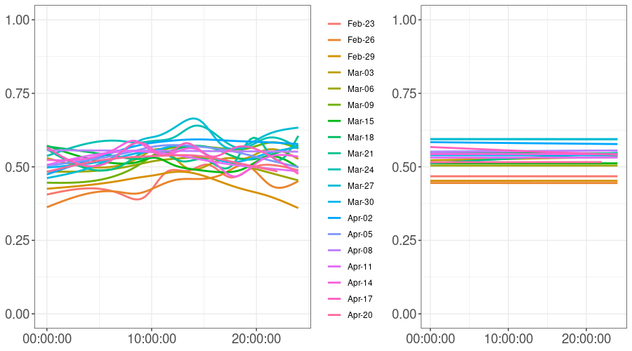
Figure 1: Smoothed daily estimate of $\psi_{n\,1}$ for the Twitter dataset (left) and for the simulated independent data (right). The daily mean rate $\widehat{p}_{0}(\ell)$ is the same for both the left and the right panel. $x$-axis: daily time. $y$-axis: cubic spline smoothing of the observed data $\xi_{n}$ and of the simulated independent data $\xi^{\prime}_{n}$.

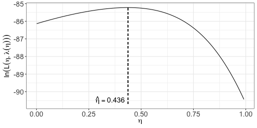
Figure 2: Plot of the function (5.3). Its maximum point gives the estimated value of the model parameter $\eta$.

Our purpose is to test the null hypothesis $H_{0}:{\boldsymbol{p_{0}}}(\ell)={\boldsymbol{p_{0}}}$ for any $\ell$. Therefore, taking $p_{0\,1}^{*}(\ell)=p_{0}^{*}=\sum_{n=1}^{N}\xi_{n}/N$ for each $\ell$, we have firstly estimated the model parameters and then we have performed the chi-squared test based on the aggregate statistics $\sum_{\ell=1}^{L}Q_{\ell}$ and its corresponding asymptotic distribution $\Gamma(\frac{(L-1)(k-1)}{2},\frac{1}{2\lambda})$. The estimated values are $\widehat{\eta}=0.4363572$ and $\widehat{\lambda}=2.728098$ (in Fig. 2 we plot the function (5.3)).

Date	$\mathrm{Obs}_{+}$	$\mathrm{Obs}_{-}$	$\mathrm{Exp}_{+}$	$\mathrm{Exp}_{-}$	$\chi^{2}_{+}$	$\chi^{2}_{-}$	${\chi^{2}_{+}}^{(c)}$	${\chi^{2}_{-}}^{(c)}$
2020-02-20	25	43	35.11	32.89	2.91	3.11	0.46	0.49
2020-02-23	53564	60476	58886.18	55153.82	481.02	513.58	2.99	3.19
2020-02-26	29831	37175	34599.51	32406.49	657.20	701.67	5.15	5.50
2020-02-29	18220	22184	20863.18	19540.82	334.87	357.53	3.27	3.49
2020-03-03	16801	14834	16335.18	15299.82	13.28	14.18	0.14	0.15
2020-03-06	27906	27030	28366.99	26569.01	7.49	8.00	0.06	0.07
2020-03-09	41650	34769	39460.04	36958.96	121.54	129.76	0.90	0.96
2020-03-12	255	156	212.23	198.77	8.62	9.20	0.62	0.67
2020-03-15	14193	13562	14331.69	13423.31	1.34	1.43	0.02	0.02
2020-03-18	12064	10089	11439.02	10713.98	34.15	36.46	0.43	0.46
2020-03-21	11571	10026	11151.92	10445.08	15.75	16.81	0.20	0.22
2020-03-24	13339	9172	11623.88	10887.12	253.07	270.20	3.19	3.41
2020-03-27	14798	10039	12824.94	12012.06	303.55	324.09	3.67	3.92
2020-03-30	12689	10651	12051.94	11288.06	33.67	35.95	0.42	0.45
2020-04-02	12714	9300	11367.24	10646.76	159.56	170.36	2.03	2.17
2020-04-05	13373	10815	12489.82	11698.18	62.45	66.68	0.76	0.82
2020-04-08	14889	11987	13877.81	12998.19	73.68	78.67	0.86	0.92
2020-04-11	12153	10777	11840.23	11089.77	8.26	8.82	0.10	0.11
2020-04-14	13406	11430	12824.42	12011.58	26.37	28.16	0.32	0.34
2020-04-17	13977	11371	13088.80	12259.20	60.27	64.35	0.72	0.77
2020-04-20	13753	12393	13500.86	12645.14	4.71	5.03	0.06	0.06

Table 1: Contingency table associated to COVID-Twitter data: $\mathrm{Obs}_{+}$ ($\mathrm{Obs}_{-}$) are the number of posts with positive (negative) sentiment posted in the day $\ell$ reported in the first column (DataTime); $\mathrm{Exp}_{+}$ ($\mathrm{Exp}_{-}$) corresponds to $N_{\ell}p_{0}^{*}$ (resp. $N_{\ell}(1-p_{0}^{*})$), where $N_{\ell}=\mathrm{Obs}_{+}+\mathrm{Obs}_{-}$; $\chi^{2}_{+}$ ($\chi^{2}_{-}$) is the quantity ($\mathrm{Obs}_{+}-\mathrm{Exp}_{+})^{2}/\mathrm{Exp}_{+}$ (resp. $(\mathrm{Obs}_{-}-\mathrm{Exp}_{-})^{2}/\mathrm{Exp}_{-}$); ${\chi^{2}_{+}}^{(c)}$ (${\chi^{2}_{-}}^{(c)}$) is the quantity $\chi^{2}_{+}/N_{\ell}^{\widehat{\eta}}$ (resp. $\chi^{2}_{-}/N_{\ell}^{\widehat{\eta}}$). The statistics $Q_{\ell}$ corresponds to ${\chi^{2}_{+}}^{(c)}+{\chi^{2}_{-}}^{(c)}$.

The contingency table and the associated statistics for testing $H_{0}$ is given in Table 1. The obtained $\chi^{2}$-statistics for a usual $\chi^{2}$-test is $5507.803$, which is significant at any level of confidence. Under the proposed GRP model and the null hypothesis, the aggregate statistics $\sum_{\ell=1}^{L}Q_{\ell}$ has (asymptotic) distribution $\Gamma(\frac{L-1}{2},\frac{1}{2\widehat{\lambda}})$ and the corresponding $p$-value associated to the data is equal to $0.4579297$. The null hypothesis that the daily long-run sentiment rate of the posts is the same for all the considered days is therefore strongly rejected with a classical $\chi^{2}$ test, while the same hypothesis is accepted if we take into account the reinforcement mechanism of correlation given in GRP model.
In Fig. 3 there are the values of the single statistics $Q_{\ell}$ compared to the $95th$-quantile of the distribution $\Gamma(\frac{1}{2},\frac{1}{2\widehat{\lambda}})$.

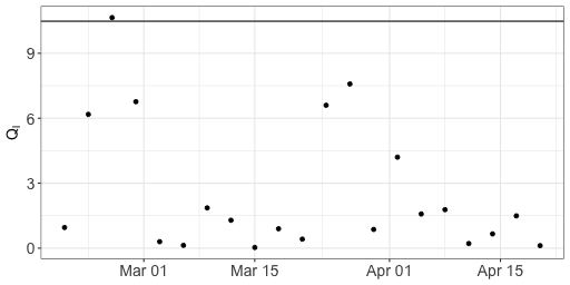
Figure 3: Plot of the $Q_{\ell}$-series. The black line corresponds to the value of $95th$-quantile of the distribution $\Gamma(\frac{1}{2},\frac{1}{2\widehat{\lambda}})$, that is $10.48$.

Df	1	2	3	4	5	6	7	8	9	10
$\chi^{2}$	3.454	3.624	4.209	4.640	5.065	7.103	8.660	8.812	10.360	12.852
$p\mathrm{-value}$	0.063	0.163	0.240	0.326	0.408	0.311	0.278	0.358	0.322	0.232

Table 2: Summary of Ljung–Box test for autocorrelation of $\{Q_{\ell}:\,\ell=1,\dots,21\}$, with different numbers of autocorrelation lags being tested. Df: number of lags under investigation; $\chi^{2}$: Ljung–Box test statistics, which is distributed as a $\chi^{2}$ distribution with Df degrees of freedom under the null hypothesis of independence; $p\mathrm{-value}$: $p\mathrm{-value}$ of the Ljung–Box test.
The strong emotional involvement of the considered period had a “mixing effect” that cancelled possible significant autocorrelation during different 3-delayed days.

7 Asymptotic results for the empirical means

Theorem 4.1 is a consequence of the following Proposition7.1 and Theorem 7.2 for the empirical means ${\boldsymbol{\overline{\xi}_{N}}}$. In the sequel, we will use the symbol $\stackrel{{\scriptstyle s}}{{\longrightarrow}}$ in order to denote the stable convergence (for a brief review on stable convergence, see Section S6).

Leveraging the Stochastic Approximation results collected in Section S5, we prove in Section S1.3 the following result:

Proposition 7.1.

Take $\epsilon_{n}=(n+1)^{-\epsilon}$ and $\delta_{n}=c\epsilon_{n}$, with $\epsilon\in(0,1]$ and $c>0$, and set $\Gamma=\mathrm{diag}({{\boldsymbol{p_{0}}}})-{{\boldsymbol{p_{0}}}}{{\boldsymbol{p_{0}}}^{\top}}$. Then ${\boldsymbol{\overline{\xi}_{N}}}\stackrel{{\scriptstyle a.s.}}{{\longrightarrow}}{\boldsymbol{p_{0}}}$ and

$$\sqrt{N}\left({\boldsymbol{\overline{\xi}_{N}}}-{\boldsymbol{p_{0}}}\right)\stackrel{{\scriptstyle s}}{{\longrightarrow}}\mathcal{N}\left({\boldsymbol{0}},\lambda\Gamma\right),$$

with $\lambda=(c+1)^{2}$ when $0<\epsilon<1$ and $\lambda=(c+1)^{2}+c^{2}=2c(c+1)+1$ when $\epsilon=1$.

For the case when $(\epsilon_{n})_{n}$ and $(\delta_{n})_{n}$ in (2.7) go to zero with different rates, we prove the following theorem (the proof is illustrated in Section 8):

Theorem 7.2.

Take $\epsilon_{n}=(n+1)^{-\epsilon}$ and $\delta_{n}\sim c(n+1)^{-\delta}$, with $\epsilon\in(0,1)$, $\delta\in(\epsilon/2,\epsilon)$ and $c>0$. Then ${\boldsymbol{\overline{\xi}_{N}}}\stackrel{{\scriptstyle a.s.}}{{\longrightarrow}}{\boldsymbol{p_{0}}}$ and

$$N^{1/2-(\epsilon-\delta)}\left({\boldsymbol{\overline{\xi}_{N}}}-{\boldsymbol{p_{0}}}\right)\stackrel{{\scriptstyle s}}{{\longrightarrow}}\mathcal{N}\left({\boldsymbol{0}},\frac{c^{2}}{1+2(\epsilon-\delta)}\Gamma\right),$$

with $\Gamma=\mathrm{diag}({{\boldsymbol{p_{0}}}})-{{\boldsymbol{p_{0}}}}{{\boldsymbol{p_{0}}}^{\top}}$.

In the framework of the above theorem, we can distinguish the following two cases:

• $\epsilon\in(1/2,1)$ and $\delta\in(1/2,\epsilon)$ or

• $\epsilon\in(0,1)$ and $\delta\in(\epsilon/2,\min\{\epsilon,1/2\}]\setminus\{\epsilon\}$.

In case 1), we have $\sum_{n}\epsilon_{n}=+\infty$, $\sum_{n}\epsilon_{n}^{2}<+\infty$ and $\sum_{n}\delta_{n}^{2}<+\infty$ and so the typical asymptotic behaviour of the predictive mean of an urn process, that is its almost sure convergence. In case 2), we have $\sum_{n}\epsilon_{n}=+\infty$ and $\sum_{n}\delta_{n}^{2}=+\infty$ (while the series $\sum_{n}\epsilon_{n}^{2}$ may be convergent or divergent) and it seems to us not immediate to check the convergence of the predict means. Therefore, for the proof of Theorem 7.2 in this last case, we will employ a different technique, which is based on the $L^{2}$-estimate of Lemma 8.1 for the predictive mean ${\boldsymbol{\psi_{N}}}$ and the almost sure convergence of the corresponding empirical mean ${\boldsymbol{\overline{\psi}_{N-1}}}$.

8 Proof of Theorem 7.2

For all the sequel, we set ${\boldsymbol{\overline{\psi}_{N-1}}}=\sum_{n=1}^{N}{\boldsymbol{\psi_{n-1}}}/N$ and ${\boldsymbol{\overline{\theta}_{N-1}}}=\sum_{n=1}^{N}{\boldsymbol{\theta_{n-1}}}/N$. To the proof of Theorem 7.2, we premise some intermediate results.

Lemma 8.1.

Under the same assumptions of Theorem 7.2, we have $E[\|{\boldsymbol{\theta_{n}}}\|^{2}]=O(n^{\epsilon-2\delta})\to 0$.

Proof.

We observe that, starting from (2.7), we get

$$\|{\boldsymbol{\theta_{n+1}}}\|^{2}={\boldsymbol{\theta_{n+1}}}^{\top}{\boldsymbol{\theta_{n+1}}}=(1-\epsilon_{n})^{2}\|{\boldsymbol{\theta_{n}}}\|^{2}+\delta_{n}^{2}\|\Delta{\boldsymbol{M_{n+1}}}\|^{2}+2(1-\epsilon_{n})\delta_{n}{\boldsymbol{\theta_{n}}}^{\top}\Delta{\boldsymbol{M_{n+1}}}$$

and so

$$E[\|{\boldsymbol{\theta_{n+1}}}\|^{2}|\mathcal{F}_{n}]=(1-\epsilon_{n})^{2}\|{\boldsymbol{\theta_{n}}}\|^{2}+\delta_{n}^{2}E[\|\Delta{\boldsymbol{M_{n+1}}}\|^{2}|\mathcal{F}_{n}]\,.$$ (8.1)

Hence, setting $x_{n}=E[\|{\boldsymbol{\theta_{n}}}\|^{2}]$, we get

$$\begin{split}x_{n+1}&=(1-2\epsilon_{n})x_{n}+\epsilon_{n}^{2}x_{n}+\delta_{n}^{2}E[\|\Delta{\boldsymbol{M_{n+1}}}\|^{2}]\\ &=(1-2\epsilon_{n})x_{n}+\epsilon_{n}\left(\epsilon_{n}x_{n}+\frac{\delta_{n}^{2}}{\epsilon_{n}}E[\|\Delta{\boldsymbol{M_{n+1}}}\|^{2}]\right)\\ &=(1-2\epsilon_{n})x_{n}+2\epsilon_{n}\zeta_{n},\end{split}$$

with $0\leq\zeta_{n}=\left(\epsilon_{n}x_{n}+\frac{\delta_{n}^{2}}{\epsilon_{n}}E[\|\Delta{\boldsymbol{M_{n+1}}}\|^{2}]\right)/2$. Applying Lemma S4.4 (with $\gamma_{n}=2\epsilon_{n}$), we find that $\limsup_{n}x_{n}\leq\limsup_{n}\zeta_{n}$. On the other hand, since $(\Delta{\boldsymbol{M_{n+1}}})_{n}$ is uniformly bounded and $\epsilon_{n}^{2}/\delta_{n}^{2}\sim c^{-2}n^{-2(\epsilon-\delta)}\to 0$, we have $\zeta_{n}=O(\epsilon_{n}+\delta_{n}^{2}\epsilon_{n}^{-1})=O(\delta_{n}^{2}/\epsilon_{n})$ and so $x_{n}=O(\delta_{n}^{2}/\epsilon_{n})$. We can conclude recalling that $\delta_{n}^{2}/\epsilon_{n}\sim c^{2}n^{\epsilon-2\delta}$. ∎

Lemma 8.2.

Under the same assumptions of Theorem 7.2, we have

$${\boldsymbol{\overline{\theta}_{N-1}}}=\frac{1}{N}\sum_{n=1}^{N}{\boldsymbol{\theta_{n-1}}}=\frac{1}{N}\sum_{n=0}^{N-1}\frac{\delta_{n}}{\epsilon_{n}}\Delta{\boldsymbol{M_{n+1}}}+{\boldsymbol{R_{N}}}\,,$$ (8.2)

where ${\boldsymbol{R_{N}}}\stackrel{{\scriptstyle a.s.}}{{\longrightarrow}}{\boldsymbol{0}}$ and $N^{e}E\big{[}\,|{\boldsymbol{R_{N}}}|\,\big{]}\longrightarrow 0$ with $e=1/2-(\epsilon-\delta)\in(0,1/2)$.

Proof.

By (2.8), we have

$${\boldsymbol{\theta_{n}}}=-\frac{1}{\epsilon_{n}}\left({\boldsymbol{\theta_{n+1}}}-{\boldsymbol{\theta_{n}}}\right)+\frac{\delta_{n}}{\epsilon_{n}}\Delta{\boldsymbol{M_{n+1}}}.$$

Therefore, we can write

$$\begin{split}\sum_{n=0}^{N-1}{\boldsymbol{\theta_{n}}}&=-\sum_{n=0}^{N-1}\frac{1}{\epsilon_{n}}\left({\boldsymbol{\theta_{n+1}}}-{\boldsymbol{\theta_{n}}}\right)+\sum_{n=0}^{N-1}\frac{\delta_{n}}{\epsilon_{n}}\Delta{\boldsymbol{M_{n+1}}}\\ &=-\left(\frac{{\boldsymbol{\theta_{N}}}}{\epsilon_{N-1}}-\frac{{\boldsymbol{\theta_{0}}}}{\epsilon_{0}}\right)-\sum_{n=1}^{N-1}\left(\frac{1}{\epsilon_{n-1}}-\frac{1}{\epsilon_{n}}\right){\boldsymbol{\theta_{n}}}+\sum_{n=0}^{N-1}\frac{\delta_{n}}{\epsilon_{n}}\Delta{\boldsymbol{M_{n+1}}}\,,\end{split}$$

where the second equality is due to the Abel transformation for a series. It follows the decomposition (8.2) with

$${\boldsymbol{R_{N}}}=-\frac{1}{N}\left(\frac{{\boldsymbol{\theta_{N}}}}{\epsilon_{N-1}}-\frac{{\boldsymbol{\theta_{0}}}}{\epsilon_{0}}\right)-\frac{1}{N}\sum_{n=1}^{N-1}\left(\frac{1}{\epsilon_{n-1}}-\frac{1}{\epsilon_{n}}\right){\boldsymbol{\theta_{n}}}\,.$$ (8.3)

Since $|{\boldsymbol{\theta_{n}}}|=O(1)$, we have

$$|{\boldsymbol{R_{N}}}|=O(N^{-1}\epsilon_{N-1}^{-1})+O\left(N^{-1}\sum_{n=1}^{N-1}|\epsilon_{n-1}^{-1}-\epsilon_{n}^{-1}|\right)$$

Note that $\sum_{n=1}^{N-1}|\epsilon_{n-1}^{-1}-\epsilon_{n}^{-1}|=\epsilon_{0}^{-1}-\epsilon_{N-1}^{-1}$ when $(\epsilon_{n})$ is decreasing and so the last term in the above expression is $O(N^{-1}\epsilon_{N-1}^{-1})$. Therefore, since $\epsilon<1$ by assumption, we have $|{\boldsymbol{R_{N}}}|=O(N^{-(1-\epsilon)})\to 0$.
Regarding the last statement of the lemma, we observe that, from what we have proven before, we obtain $N^{e}E\big{[}|{\boldsymbol{R_{N}}}|\big{]}=O(N^{e-(1-\epsilon)})=O(N^{\delta-1/2})\to 0$ when $\delta<1/2$. However, in the considered cases 1) and 2), we might have $\delta\geq 1/2$. Therefore, we need other arguments in order to prove the last statement. To this purpose, we observe that, by Lemma 8.1, we have $E[\,|{\boldsymbol{\theta_{n}}}|\,]=O(n^{\epsilon/2-\delta})$ and so, by (8.3), we have

$$\begin{split}N^{e}E\big{[}\,|{\boldsymbol{R_{N}}}|\,\big{]}&=O(N^{-(1-e)}N^{3\epsilon/2-\delta})+O\left(\frac{1}{N^{1-e}}\sum_{n=1}^{N-1}|\epsilon_{n-1}^{-1}-\epsilon_{n}^{-1}|n^{\epsilon/2-\delta}\right)\\ &=O(N^{-(1-\epsilon)/2})+O\left(\frac{1}{N^{1-e}}\sum_{n=1}^{N-1}|\epsilon_{n-1}^{-1}-\epsilon_{n}^{-1}|n^{\epsilon/2-\delta}\right)\,.\end{split}$$

Moreover, we have

$$\sum_{n=1}^{N-1}|\epsilon_{n-1}^{-1}-\epsilon_{n}^{-1}|n^{\epsilon/2-\delta}=\sum_{n=1}^{N-1}\left[(n-1)^{\epsilon}-n^{\epsilon}\right]n^{\epsilon/2-\delta}=\sum_{n=1}^{N-1}n^{\epsilon-1+\epsilon/2-\delta}\sim N^{3\epsilon/2-\delta}=o(N^{1-e})\,,$$

because $e=1/2-(\epsilon-\delta)$ and $\epsilon<1$. Summing up, we have $N^{e}E[|{\boldsymbol{R_{N}}}|]=O(N^{-(1-\epsilon)/2})+o(1)\to 0$. ∎

Lemma 8.3.

Under the same assumptions of Theorem 7.2, we have ${\boldsymbol{\overline{\theta}_{N-1}}}\stackrel{{\scriptstyle a.s.}}{{\longrightarrow}}{\boldsymbol{0}}$, that is ${\boldsymbol{\overline{\psi}_{N-1}}}\stackrel{{\scriptstyle a.s.}}{{\longrightarrow}}{\boldsymbol{p_{0}}}$. In particular, when $\epsilon\in(1/2,1)$ and $\delta\in(1/2,\epsilon)$, we have ${\boldsymbol{\theta_{N}}}\stackrel{{\scriptstyle a.s.}}{{\longrightarrow}}{\boldsymbol{0}}$, that is ${\boldsymbol{\psi_{N}}}\stackrel{{\scriptstyle a.s.}}{{\longrightarrow}}{\boldsymbol{p_{0}}}$.

Proof.

Let us distinguish the following two cases:

• $\epsilon\in(1/2,1)$ and $\delta\in(1/2,\epsilon)$ or

• $\epsilon\in(0,1)$ and $\delta\in(\epsilon/2,\min\{\epsilon,1/2\}]\setminus\{\epsilon\}$.

For the case 1), we observe that, by (8.1), we have

$$E[\|{\boldsymbol{\theta_{n+1}}}\|^{2}|\mathcal{F}_{n}]\leq(1+\epsilon_{n}^{2})E[\|{\boldsymbol{\theta_{n}}}\|^{2}|\mathcal{F}_{n}]+\delta_{n}^{2}E[\|\Delta{\boldsymbol{M_{n+1}}}\|^{2}|\mathcal{F}_{n}].$$

Therefore, since $(\Delta{\boldsymbol{M_{n+1}}})_{n}$ is uniformly bounded and, in case 1), we have $\sum_{n}\epsilon_{n}^{2}<+\infty$ and $\sum_{n}\delta_{n}^{2}<+\infty$, the sequence $(\|{\boldsymbol{\theta_{n}}}\|^{2})_{n}$ is a bounded non-negative almost supermartingale. As a consequence, it converges almost surely to a certain random variable. This limit random variable is necessarily equal to ${\boldsymbol{0}}$ because, by Lemma 8.1, we have $E[\|{\boldsymbol{\theta_{n}}}\|^{2}]=O(n^{\epsilon-2\delta})\to 0$. Hence, we have the almost sure convergence of ${\boldsymbol{\theta_{N}}}$ to ${\boldsymbol{0}}$ and, consequently, the almost sure convergence of ${\boldsymbol{\overline{\theta}_{N-1}}}$ to ${\boldsymbol{0}}$ follows by Lemma S4.2 and Remark S4.3 (with $c_{n}=n$ and $v_{N,n}=n/N$), because $E[{\boldsymbol{\theta_{n-1}}}|\mathcal{F}_{n-2}]=(1-\epsilon_{n-2}){\boldsymbol{\theta_{n-2}}}\to{\boldsymbol{0}}$ almost surely.
For the case 2), we use Lemma 8.2, that gives the decomposition (8.2), with ${\boldsymbol{R_{N}}}\stackrel{{\scriptstyle a.s.}}{{\longrightarrow}}{\boldsymbol{0}}$. Indeed, by this decomposition, it is enough to prove that the term $\sum_{n=0}^{N-1}\frac{\delta_{n}}{\epsilon_{n}}\Delta{\boldsymbol{M_{n+1}}}/N$ converges almost surely to ${\boldsymbol{0}}$. To this purpose, we observe that, if we set

$${\boldsymbol{L_{n}}}=\sum_{j=1}^{n}\frac{1}{j}\frac{\delta_{j-1}}{\epsilon_{j-1}}\Delta{\boldsymbol{M_{j}}},$$

then $({\boldsymbol{L_{n}}})$ is a square integrable martingale. Indeed, we have

$$\sum_{n=1}^{+\infty}\frac{1}{n^{2}}\frac{\delta_{n-1}^{2}}{\epsilon_{n-1}^{2}}E[\|\Delta{\boldsymbol{M_{n}}}\|^{2}]=O\left(\sum_{n=1}^{+\infty}\frac{1}{n^{1+2e}}\right)<+\infty\,.$$

Therefore, $({\boldsymbol{L_{n}}})$ converges almost surely, that is we have $\sum_{n}\frac{1}{n}\frac{\delta_{n-1}}{\epsilon_{n-1}}\Delta{\boldsymbol{M_{n}}}<+\infty$ almost surely. Applying Lemma S4.1 (with $v_{N,n}=n/N$), we find

$$\frac{1}{N}\sum_{n=0}^{N-1}\frac{\delta_{n}}{\epsilon_{n}}\Delta{\boldsymbol{M_{n+1}}}=\sum_{n=1}^{N}v_{N,n}\frac{1}{n}\frac{\delta_{n-1}}{\epsilon_{n-1}}\Delta{\boldsymbol{M_{n}}}\stackrel{{\scriptstyle a.s.}}{{\longrightarrow}}{\boldsymbol{0}}$$

and so ${\boldsymbol{\overline{\theta}_{N-1}}}\stackrel{{\scriptstyle a.s.}}{{\longrightarrow}}{\boldsymbol{0}}$. ∎

Proof of Theorem 7.2. Set $e=1/2-(\epsilon-\delta)\in(0,1/2)$ and $\lambda=c^{2}/[2(1-e)]=c^{2}/[1+2(\epsilon-\delta)]$. Moreover, let us distinguish the following two cases:

• $\epsilon\in(1/2,1)$ and $\delta\in(1/2,\epsilon)$ or

• $\epsilon\in(0,1)$ and $\delta\in(\epsilon/2,\min\{\epsilon,1/2\}]\setminus\{\epsilon\}$.

Almost sure convergence: In case 1), by Lemma 8.3, ${\boldsymbol{\psi_{N}}}$ converges almost surely to ${\boldsymbol{p_{0}}}$. Therefore, the almost sure convergence of ${\boldsymbol{\overline{\xi}_{N}}}$ to ${\boldsymbol{p_{0}}}$ follows by Lemma S4.2 and Remark S4.3 (with $c_{n}=n$ and $v_{N,n}=n/N$), because $E[{\boldsymbol{\xi_{n+1}}}|\mathcal{F}_{n}]={\boldsymbol{\psi_{n}}}\to{\boldsymbol{p_{0}}}$ almost surely and $\sum_{n}E[\|{\boldsymbol{\xi_{n}}}\|^{2}]n^{-2}\leq\sum_{n}n^{-2}<+\infty$.
In case 2), we use a different argument. Take $\gamma\in[0,e)$ and set

$${\boldsymbol{L_{n}}}=\sum_{j=1}^{n}\frac{1}{j^{1-\gamma}}\frac{\delta_{j-1}}{\epsilon_{j-1}}\Delta{\boldsymbol{M_{j}}}\,.$$

Then $({\boldsymbol{L_{n}}})$ is a square integrable martingale, because we have

$$\sum_{n=1}^{+\infty}\frac{1}{n^{2-2\gamma}}\frac{\delta_{n-1}^{2}}{\epsilon_{n-1}^{2}}E[\|\Delta{\boldsymbol{M_{n}}}\|^{2}]=O\left(\sum_{n=1}^{+\infty}\frac{1}{n^{1+2e-2\gamma}}\right)<+\infty\,.$$

Therefore, $({\boldsymbol{L_{n}}})$ converges almost surely, that is we have $\sum_{n}\frac{1}{n^{1-\gamma}}\frac{\delta_{n-1}}{\epsilon_{n-1}}\Delta{\boldsymbol{M_{n}}}<+\infty$ almost surely. By Lemma S4.1 (with $v_{N,n}=(n/N)^{1-\gamma}\epsilon_{n-1}/\delta_{n-1}\sim n^{1-\gamma-\epsilon+\delta}/N^{1-\gamma}$), we get

$$\frac{1}{N^{1-\gamma}}\sum_{n=0}^{N-1}\Delta{\boldsymbol{M_{n+1}}}=\sum_{n=1}^{N}v_{N,n}\frac{1}{n^{1-\gamma}}\frac{\delta_{n-1}}{\epsilon_{n-1}}\Delta{\boldsymbol{M_{n}}}\stackrel{{\scriptstyle a.s.}}{{\longrightarrow}}{\boldsymbol{0}}.$$

Therefore, we have

$$N^{\gamma}\left({\boldsymbol{\overline{\xi}_{N}}}-{\boldsymbol{\overline{\psi}_{N-1}}}\right)=\frac{1}{N^{1-\gamma}}\sum_{n=0}^{N-1}\Delta{\boldsymbol{M_{n+1}}}\stackrel{{\scriptstyle a.s.}}{{\longrightarrow}}{\boldsymbol{0}},$$

that is $\left({\boldsymbol{\overline{\xi}_{N}}}-{\boldsymbol{\overline{\psi}_{N-1}}}\right)=o(N^{-\gamma})$ for each $\gamma\in[0,e)$. Recalling Lemma 8.3, we obtain in particular that ${\boldsymbol{\overline{\xi}_{N}}}$ converges almost surely to ${\boldsymbol{p_{0}}}$.
Second order asymptotic behaviour: We have

$$N^{e}\left({\boldsymbol{\overline{\xi}_{N}}}-{\boldsymbol{p_{0}}}\right)=N^{e}{\boldsymbol{\overline{\mu}_{N}}}=N^{e-1/2}\sqrt{N}\left({\boldsymbol{\overline{\mu}_{N}}}-{\boldsymbol{\overline{\theta}_{N-1}}}\right)+N^{e}{\boldsymbol{\overline{\theta}_{N-1}}}\,.$$ (8.4)

Moreover, by Lemma 8.1, we have

$$\begin{split}\frac{1}{N}\sum_{n=0}^{N-1}E[|{\boldsymbol{\theta_{n}}}|]&=O(N^{-1}\sum_{n=1}^{N}n^{\epsilon/2-\delta})=O(N^{-1-\delta+\epsilon/2+1})=O(N^{\epsilon/2-\delta})\to 0\,,\\ \frac{1}{N}\sum_{n=0}^{N-1}E[\|{\boldsymbol{\theta_{n}}}\|^{2}]&=O(N^{-1}\sum_{n=1}^{N}n^{\epsilon-2\delta})=O(N^{-1-2\delta+\epsilon+1})=O(N^{\epsilon-2\delta})\to 0\,,\end{split}$$

and so Theorem S1.1 holds true with $V=\Gamma$ (see Remark S1.2). Therefore, the first term in the right side of (8.4) converges in probability to ${\boldsymbol{0}}$ because $e<1/2$. Hence, if we prove that

$$N^{e}{\boldsymbol{\overline{\theta}_{N-1}}}\stackrel{{\scriptstyle s}}{{\longrightarrow}}\mathcal{N}\left({\boldsymbol{0}},\lambda\Gamma\right)\,,$$ (8.5)

then the proof is concluded.
In order to prove (8.5), we observe that, by decomposition (8.2) in Lemma 8.2, we have

$$N^{e}{\boldsymbol{\overline{\theta}_{N-1}}}=\sum_{n=1}^{N}{\boldsymbol{Y_{N,n}}}+N^{e}{\boldsymbol{R_{N}}}\,,$$

where ${\boldsymbol{Y_{N,n}}}=\frac{1}{N^{1-e}}\frac{\delta_{n-1}}{\epsilon_{n-1}}\Delta{\boldsymbol{M_{n}}}$ and $N^{e}{\boldsymbol{R_{N}}}$ converges in probability to ${\boldsymbol{0}}$ (because $N^{e}E\big{[}|{\boldsymbol{R_{N}}}|]\to 0$). Therefore, it is enough to prove that the term $\sum_{n=1}^{N}{\boldsymbol{Y_{N,n}}}$ stably converges to the Gaussian kernel $\mathcal{N}(0,\lambda\Gamma)$, with $\lambda=c^{2}/[2(1-e)]=c^{2}/[1+2(\epsilon-\delta)]$. To this purpose, we observe that $E[{\boldsymbol{Y_{N,n}}}|\mathcal{F}_{n-1}]={\boldsymbol{0}}$ and so $\sum_{n=1}^{N}{\boldsymbol{Y_{N,n}}}$ converges stably to $\mathcal{N}({\boldsymbol{0}},\lambda\Gamma)$ if the conditions (c1) and (c2) of Theorem S6.1, with $V=\lambda\Gamma$, hold true. Regarding (c1), we note that $\delta_{n-1}/\epsilon_{n-1}\sim cn^{\epsilon-\delta}=cn^{1/2-e}$ and so we have

$$\max_{1\leq n\leq N}|{\boldsymbol{Y_{N,n}}}|\leq N^{-(1-e)}\max_{1\leq n\leq N}\frac{\delta_{n-1}}{\epsilon_{n-1}}|{\boldsymbol{\xi_{n}}}-{{\boldsymbol{\psi_{n-1}}}}|\leq N^{-(1-e)}\max_{1\leq n\leq N}\frac{\delta_{n-1}}{\epsilon_{n-1}}=O(N^{-1/2})\to 0\,.$$

Condition (c2) means

$$\frac{1}{N^{2(1-e)}}\sum_{n=1}^{N}\frac{\delta_{n-1}^{2}}{\epsilon_{n-1}^{2}}({\boldsymbol{\xi_{n}}}-{{\boldsymbol{\psi_{n-1}}}})({\boldsymbol{\xi_{n}}}-{{\boldsymbol{\psi_{n-1}}}})^{\top}\stackrel{{\scriptstyle P}}{{\longrightarrow}}\lambda\Gamma.$$ (8.6)

We note that $N^{-2(1-e)}\sum_{n=1}^{N}\delta_{n-1}^{2}/\epsilon_{n-1}^{2}\to\lambda$, because $\delta_{n-1}^{2}/\epsilon_{n-1}^{2}\sim c^{2}n^{1-2e}$, and

$$E[({\boldsymbol{\xi_{n}}}-{{\boldsymbol{\psi_{n-1}}}})({\boldsymbol{\xi_{n}}}-{{\boldsymbol{\psi_{n-1}}}})^{\top}|\mathcal{F}_{n-1}]=\mathrm{diag}({{\boldsymbol{\psi_{n-1}}}})-{{\boldsymbol{\psi_{n-1}}}}{{\boldsymbol{\psi_{n-1}}}^{\top}}\,.$$

Therefore, in case 1), condition (8.6) immediately follows by the almost sure convergence of ${\boldsymbol{\psi_{n}}}$ to ${\boldsymbol{p_{0}}}$. It is enough to apply Lemma S4.2 and Remark S4.3 with $c_{n}=n$ and $v_{N,n}=n\delta_{n-1}^{2}/(N^{2(1-e)}\epsilon_{n-1}^{2})\sim c^{2}n^{1+2(\epsilon-\delta)}/N^{2-2e}=c^{2}(n/N)^{2(1-e)}$. In case 2), we apply again Lemma S4.2 with the above $c_{n}$ and $v_{N,n}$, but we note that ${\boldsymbol{\psi_{n}}}={\boldsymbol{\theta_{n}}}+{\boldsymbol{p_{0}}}$ and so condition (S4.1) in Lemma S4.2, with $V=\lambda\Gamma$, is equivalent to

$$\frac{1}{N^{2-2e}}\sum_{n=0}^{N-1}\frac{\delta_{n}^{2}}{\epsilon_{n}^{2}}{\boldsymbol{\theta_{n}}}\stackrel{{\scriptstyle P}}{{\longrightarrow}}{\boldsymbol{0}}\qquad\mbox{and}\qquad\frac{1}{N^{2-2e}}\sum_{n=0}^{N-1}\frac{\delta_{n}^{2}}{\epsilon_{n}^{2}}{\boldsymbol{\theta_{n}}}{\boldsymbol{\theta_{n}}}^{\top}\stackrel{{\scriptstyle P}}{{\longrightarrow}}0_{k\times k}.$$

These two convergences hold true because, by Lemma 8.1, we have

$$\begin{split}\frac{1}{N^{2-2e}}\sum_{n=0}^{N-1}\frac{\delta_{n}^{2}}{\epsilon_{n}^{2}}E[|{\boldsymbol{\theta_{n}}}|]&=O(N^{-2+2e}\sum_{n=1}^{N}n^{-2\delta+2\epsilon-\delta+\epsilon/2})=O(N^{-2+2e-3\delta+5\epsilon/2+1})=O(N^{-\delta+\epsilon/2})\to 0\,,\\ \frac{1}{N^{2-2e}}\sum_{n=0}^{N-1}\frac{\delta_{n}^{2}}{\epsilon_{n}^{2}}E[\|{\boldsymbol{\theta_{n}}}\|^{2}]&=O(N^{-2+2e}\sum_{n=1}^{N}n^{-2\delta+2\epsilon-2\delta+\epsilon})=O(N^{-2+2e-4\delta+3\epsilon+1})=O(N^{-2\delta+\epsilon})\to 0\,.\end{split}$$

Therefore, in both cases 1) and 2), conditions c1) and c2) of Theorem S6.1 are satisfied and so $\sum_{n=1}^{N}{\boldsymbol{Y_{N,n}}}$ stably converges to the Gaussian kernel $\mathcal{N}(0,\lambda\Gamma)$. ∎

Declaration

Both authors equally contributed to this work.

Acknowledgments

Giacomo Aletti is a member of the Italian Group “Gruppo Nazionale per il Calcolo Scientifico” of the Italian Institute “Istituto Nazionale di Alta Matematica” and Irene Crimaldi is a member of the Italian Group “Gruppo Nazionale per l’Analisi Matematica, la Probabilità e le loro Applicazioni” of the Italian Institute “Istituto Nazionale di Alta Matematica”.

Funding Sources

Irene Crimaldi is partially supported by the Italian “Programma di Attività Integrata” (PAI), project “TOol for Fighting FakEs” (TOFFE) funded by IMT School for Advanced Studies Lucca.

SM Supplemental Materials

In this document we collect some proofs, complements, technical results and recalls, useful for [2]. Therefore, the notation and the assumptions used here are the same as those used in that paper.

Appendix S1 Proofs and intermediate results

We here collect some proofs omitted in the main text of the paper [2].

S1.1 Proof of Theorem 4.1

The proof is based on Proposition 7.1 (for case a)) and Theorem 7.2 (for case b)). The almost sure convergence of $O_{i}/N$ immediately follows since $O_{i}/N=\overline{\xi}_{N\,i}$. In order to prove the stated convergence in distribution, we mimic the classical proof for the Pearson chi-squared test based on the Sherman Morison formula (see [18]), but see also [16, Corollary 2].

We start recalling the Sherman Morison formula: if $A$ is an invertible square matrix and we have $1-{\boldsymbol{v}}^{\top}A^{-1}{\boldsymbol{u}}\neq 0$, then

$$(A-{\boldsymbol{u}}{\boldsymbol{v}}^{\top})^{-1}=A^{-1}+\frac{A^{-1}{\boldsymbol{u}}{\boldsymbol{v}}^{\top}A^{-1}}{1-{\boldsymbol{v}}^{\top}A^{-1}{\boldsymbol{u}}}.$$

Given the observation ${\boldsymbol{\xi_{n}}}=(\xi_{n\,1},\dots,\xi_{n\,k})^{\top}$, we define the “truncated” vector ${\boldsymbol{\xi^{*}_{n}}}=(\xi^{*}_{n\,1},\ldots,\xi^{*}_{n\,k-1})^{\top}$, given by the first $k-1$ components of ${\boldsymbol{\xi_{n}}}$. Proposition 7.1 (for case a)) and Theorem 7.2 (for case b)) give the second order asymptotic behaviour of $({\boldsymbol{\xi_{n}}})$, that immediately implies

$$N^{e}\left({\boldsymbol{\overline{\xi}^{*}_{N}}}-{\boldsymbol{p^{*}}}\right)=\frac{\sum_{n=1}^{N}({\boldsymbol{\xi^{*}_{n}}}-{\boldsymbol{p^{*}}})}{N^{1-e}}\mathop{\longrightarrow}^{d}\mathcal{N}({\boldsymbol{0}},\Gamma_{*}),$$ (S1.1)

where ${\boldsymbol{p^{*}}}$ is given by the first $k-1$ components of ${\boldsymbol{p_{0}}}$ and $\Gamma_{*}=\lambda(\mathrm{diag}({\boldsymbol{p^{*}}})-{\boldsymbol{p^{*}}}{\boldsymbol{p^{*}}}^{T})$. By assumption $p_{0\,i}>0$ for all $i=1,\dots,k$ and so $\mathrm{diag}({\boldsymbol{p^{*}}})$ is invertible with inverse $\mathrm{diag}({\boldsymbol{p^{*}}})^{-1}=\mathrm{diag}(\frac{1}{p_{0\,1}},\ldots,\frac{1}{p_{0\,k-1}})$ and, since $(\mathrm{diag}({\boldsymbol{p^{*}}})^{-1}){\boldsymbol{p^{*}}}={\boldsymbol{1}}\in\mathbb{\mathbb{R}}^{k-1}$, we have

$$1-{\boldsymbol{p^{*}}}^{T}\mathrm{diag}({\boldsymbol{p^{*}}})^{-1}{\boldsymbol{p^{*}}}=1-\sum_{i=1}^{k-1}p_{0\,i}=\sum_{i=1}^{k}p_{0\,i}-\sum_{i=1}^{k-1}p_{0\,i}=p_{0\,k}>0.$$

Therefore we can use the Sherman Morison formula with $A=\mathrm{diag}({\boldsymbol{p^{*}}})$ and ${\boldsymbol{u}}={\boldsymbol{v}}={\boldsymbol{p^{*}}}$, and we obtain

$$(\Gamma_{*})^{-1}=\frac{1}{\lambda}(\mathrm{diag}({\boldsymbol{p^{*}}})-{\boldsymbol{p^{*}}}{\boldsymbol{p^{*}}}^{T})^{-1}=\frac{1}{\lambda}\Big{(}\mathrm{diag}(\tfrac{1}{p_{0\,1}},\ldots,\tfrac{1}{p_{0\,k-1}})+\frac{1}{p_{0\,k}}{\boldsymbol{1}}{\boldsymbol{1}}^{\top}\Big{)}.$$ (S1.2)

Now, since $\sum_{i=1}^{k}(\overline{\xi}_{N\,i}-{p_{0\,i}})=0$, then $\overline{\xi}_{N\,k}-{p_{0\,k}}=\sum_{i=1}^{k-1}(\overline{\xi}_{N\,i}-{p_{0\,i}})$ and so we get

$$\sum_{i=1}^{k}\frac{(O_{i}-N{p_{0\,i}})^{2}}{N{p_{0\,i}}} =N\sum_{i=1}^{k}\frac{(\overline{\xi}_{N\,i}-{p_{0\,i}})^{2}}{{p_{0\,i}}}=N\Big{[}\sum_{i=1}^{k-1}\frac{(\overline{\xi}_{N\,i}-{p_{0\,i}})^{2}}{{p_{0\,i}}}+\frac{(\overline{\xi}_{N\,k}-{p_{0\,k}})^{2}}{{p_{0\,k}}}\Big{]}$$

$$=N\Big{[}\sum_{i=1}^{k-1}\frac{(\overline{\xi}_{N\,i}-{p_{0\,i}})^{2}}{{p_{0\,i}}}+\frac{(\sum_{i=1}^{k-1}(\overline{\xi}_{N\,i}-{p_{0\,i}}))^{2}}{{p_{0\,k}}}\Big{]}$$

$$=N\sum_{i_{1},i_{2}=1}^{k-1}(\overline{\xi}_{N\,{i_{1}}}-{p_{0\,i_{1}}})(\overline{\xi}_{N\,i_{2}}-{p_{0\,i_{2}}})\Big{(}I_{i_{1},i_{2}}\frac{1}{{p_{0\,i_{1}}}}+\frac{1}{{p_{0\,k}}}\Big{)},$$

where $I_{i_{1}\,i_{2}}$ is equal to $1$ if $i_{1}=i_{2}$ and equal to zero otherwise. Finally, from the above equalities, recalling (S1.1) and (S1.2), we obtain

$$\frac{1}{N^{1-2e}}\sum_{i=1}^{k}\frac{(O_{i}-N{p_{0\,i}})^{2}}{N{p_{0\,i}}}=\lambda N^{2e}({\boldsymbol{\overline{\xi}^{*}_{N}}}-{\boldsymbol{p^{*}}})^{\top}(\Gamma_{*})^{-1}({\boldsymbol{\overline{\xi}^{*}_{N}}}-{\boldsymbol{p^{*}}})\mathop{\longrightarrow}\limits^{d}\lambda W_{0}=W_{*},$$

where $1-2e\geq 0$ and $W_{0}$ is a random variable with distribution $\chi^{2}(k-1)=\Gamma((k-1)/2,1/2)$, where $\Gamma(a,b)$ denotes the Gamma distribution with density function

$$f(w)=\frac{b^{a}}{\Gamma(a)}w^{a-1}e^{-bw}.$$

As a consequence, $W_{*}$ has distribution $\Gamma((k-1)/2,1/(2\lambda))$.

S1.2 A preliminary central limit theorem

The following preliminary central limit theorem is useful for the proofs of the other central limit theorems stated in [2] and in Section S2.

Theorem S1.1.

If

$$\frac{1}{N}\sum_{n=1}^{N}\mathrm{diag}({{\boldsymbol{\psi_{n-1}}}})-{{\boldsymbol{\psi_{n-1}}}}{{\boldsymbol{\psi_{n-1}}}^{\top}}\mathop{\longrightarrow}\limits^{P}V\,,$$ (S1.3)

where $V$ is a random variable with values in the space of positive semidefinite $k\times k$-matrices, then

$$\sqrt{N}\left({\boldsymbol{\overline{\mu}_{N}}}-{\boldsymbol{\overline{\theta}_{N-1}}}\right)=\sqrt{N}\left({\boldsymbol{\overline{\xi}_{N}}}-{\boldsymbol{\overline{\psi}_{N-1}}}\right)\stackrel{{\scriptstyle s}}{{\longrightarrow}}\mathcal{N}\left({\boldsymbol{0}},V\right).$$

Proof.

We can write

$$\begin{split}\sqrt{N}\left({\boldsymbol{\overline{\xi}_{N}}}-{\boldsymbol{\overline{\psi}_{N-1}}}\right)&=\frac{1}{\sqrt{N}}N\left({\boldsymbol{\overline{\xi}_{N}}}-{\boldsymbol{\overline{\psi}_{N-1}}}\right)=\frac{1}{\sqrt{N}}\sum_{n=1}^{N}({\boldsymbol{\xi_{n}}}-{\boldsymbol{\psi_{n-1}}})\\ &=\frac{1}{\sqrt{N}}\sum_{n=1}^{N}\Delta{\boldsymbol{M_{n}}}=\sum_{n=1}^{N}Y_{N,n},\end{split}$$

with ${\boldsymbol{Y_{N,n}}}=N^{-1/2}\Delta{\boldsymbol{M_{n}}}$. For the convergence of $\sum_{n=1}^{N}{\boldsymbol{Y_{N,n}}}$, we observe that $E[{\boldsymbol{Y_{N,k}}}|\mathcal{F}_{k-1}]={\boldsymbol{0}}$ and so, by Theorem S6.1, it converges stably to $\mathcal{N}({\boldsymbol{0}},V)$ if the conditions (c1) and (c2) hold true. Regarding (c1), we note that $\max_{1\leq n\leq N}|{\boldsymbol{Y_{N,n}}}|\leq\frac{1}{\sqrt{N}}\max_{1\leq n\leq N}|{\boldsymbol{\xi_{n}}}-{{\boldsymbol{\psi_{n-1}}}}|=O(1/\sqrt{N})\to 0$. Condition (c2) means

$$\sum_{n=1}^{N}{\boldsymbol{Y_{N,n}}}{{\boldsymbol{Y}}_{{\boldsymbol{N,n}}}^{\top}}=\frac{1}{N}\sum_{n=1}^{N}({\boldsymbol{\xi_{n}}}-{{\boldsymbol{\psi_{n-1}}}})({\boldsymbol{\xi_{n}}}-{{\boldsymbol{\psi_{n-1}}}})^{\top}\stackrel{{\scriptstyle P}}{{\longrightarrow}}V.$$

The above convergence holds true by Assumption (S1.3) and Lemma S4.2 (with $c_{n}=n$ and $v_{N,n}=n/N$). Indeed, we have $\sum_{n\geq 1}E[\|{\boldsymbol{\xi_{n}}}-{{\boldsymbol{\psi_{n-1}}}}\|^{2}]/n^{2}\leq\sum_{n\geq 1}n^{-2}<+\infty$ and

$$E[({\boldsymbol{\xi_{n}}}-{{\boldsymbol{\psi_{n-1}}}})({\boldsymbol{\xi_{n}}}-{{\boldsymbol{\psi_{n-1}}}})^{\top}|\mathcal{F}_{n-1}]=\mathrm{diag}({{\boldsymbol{\psi_{n-1}}}})-{{\boldsymbol{\psi_{n-1}}}}{{\boldsymbol{\psi_{n-1}}}^{\top}}\,.$$

∎

Remark S1.2.

Recalling that ${\boldsymbol{\psi_{n}}}={\boldsymbol{\theta_{n}}}+{\boldsymbol{p_{0}}}$, the convergence (S1.3) with $V=\Gamma=\mathrm{diag}({{\boldsymbol{p_{0}}}})-{{\boldsymbol{p_{0}}}}{{\boldsymbol{p_{0}}}^{\top}}$, means

$${\boldsymbol{\overline{\theta}_{N-1}}}=\frac{1}{N}\sum_{n=1}^{N}{\boldsymbol{\theta_{n-1}}}\stackrel{{\scriptstyle P}}{{\longrightarrow}}{\boldsymbol{0}}\qquad\mbox{and}\qquad\frac{1}{N}\sum_{n=1}^{N}{\boldsymbol{\theta_{n-1}}}{\boldsymbol{\theta_{n-1}}}^{\top}\stackrel{{\scriptstyle P}}{{\longrightarrow}}0_{k\times k}\,,$$

where $0_{k\times k}$ is the null matrix with dimension $k\times k$.

S1.3 Proof of Proposition 7.1

By Lemma S4.2 (with $c_{n}=n$ and $v_{N,n}=n/N$), Remark S4.3 and Theorem S5.1, we immediately get ${\boldsymbol{\overline{\xi}_{N}}}\to{\boldsymbol{p_{0}}}$ almost surely. Indeed, we have $E[{\boldsymbol{\xi_{n+1}}}|\mathcal{F}_{n}]={\boldsymbol{\psi_{n}}}\to{\boldsymbol{p_{0}}}$ almost surely and $\sum_{n\geq 1}E[\|{\boldsymbol{\xi_{n}}}\|^{2}]n^{-2}\leq\sum_{n\geq 1}n^{-2}<+\infty$.
Regarding the central limit theorem for ${\boldsymbol{\overline{\xi}_{N}}}$, we have to distinguish the two cases $1/2<\epsilon\leq 1$ or $0<\epsilon\leq 1/2$. In the first case, the result follows from Theorem S5.3, because (2.9) and the fact that $E[\Delta{\boldsymbol{M_{n+1}}}\Delta{\boldsymbol{M_{n+1}}}^{\top}\,|\mathcal{F}_{n}]=\mathrm{diag}({{\boldsymbol{\psi_{n-1}}}})-{{\boldsymbol{\psi_{n-1}}}}{{\boldsymbol{\psi_{n-1}}}^{\top}}\to\Gamma$ almost surely; while for the second case the result follows from Theorem S1.1. Indeed, we have

$$\begin{split}\sqrt{N}\left({\boldsymbol{\overline{\xi}_{N}}}-{\boldsymbol{p_{0}}}\right)&=\sqrt{N}\left({\boldsymbol{\overline{\xi}_{N}}}-{\boldsymbol{\overline{\psi}_{N-1}}}\right)+\sqrt{N}\left({\boldsymbol{\overline{\psi}_{N-1}}}-{\boldsymbol{p_{0}}}\right)\\ &=(c+1)\sqrt{N}\left({\boldsymbol{\overline{\xi}_{N}}}-{\boldsymbol{\overline{\psi}_{N-1}}}\right)-\sqrt{N}{\boldsymbol{D_{N}}},\end{split}$$

where ${{\boldsymbol{D}}_{N}}=c\left({\boldsymbol{\overline{\xi}_{N}}}-{\boldsymbol{\overline{\psi}_{N-1}}}\right)-\left({\boldsymbol{\overline{\psi}_{N-1}}}-{\boldsymbol{p_{0}}}\right)$. By Theorem S1.1, the term $(c+1)\sqrt{N}\left({\boldsymbol{\overline{\xi}_{N}}}-{\boldsymbol{\overline{\psi}_{N-1}}}\right)$ stably converges to $\mathcal{N}(0,(c+1)^{2}\Gamma)$ (note that assumption (S1.3) is satisfied with $V=\Gamma$, because ${\boldsymbol{\psi_{n}}}\to{\boldsymbol{p_{0}}}$ almost surely). Therefore, in order to conclude, it is enough to show that $\sqrt{N}{\boldsymbol{D_{N}}}$ converges in probability to ${\boldsymbol{0}}$. To this purpose, we observe that, by (2.7) with $\delta_{n}=c\epsilon_{n}$, we have

$${\boldsymbol{\psi_{n}}}-{\boldsymbol{\psi_{n-1}}}=\epsilon_{n-1}\left[c({\boldsymbol{\xi_{n}}}-{\boldsymbol{\psi_{n-1}}})-({\boldsymbol{\psi_{n-1}}}-{\boldsymbol{p_{0}}})\right]$$

and so

$$\begin{split}{{\boldsymbol{D}}_{N}}=\frac{1}{N}\sum_{n=1}^{N}\frac{{\boldsymbol{\psi_{n}}}-{\boldsymbol{\psi_{n-1}}}}{\epsilon_{n-1}}.\end{split}$$

Moreover, we note that $\sum_{n=1}^{+\infty}({\boldsymbol{\psi_{n}}}-{\boldsymbol{\psi_{n-1}}})=\lim_{N}{\boldsymbol{\psi_{N}}}-{\boldsymbol{\psi_{0}}}={\boldsymbol{p_{0}}}-{\boldsymbol{\psi_{0}}}<+\infty$ and, by Lemma S4.1 (with $v_{N,n}=\epsilon_{N-1}/\epsilon_{n-1}$), we get

$$\epsilon_{N-1}\sum_{n=1}^{N}\frac{{\boldsymbol{\psi_{n}}}-{\boldsymbol{\psi_{n-1}}}}{\epsilon_{n-1}}\stackrel{{\scriptstyle a.s.}}{{\longrightarrow}}{\boldsymbol{0}}.$$

For $\epsilon\leq 1/2$, this fact implies

$$\sqrt{N}{\boldsymbol{D_{N}}}=\frac{1}{\sqrt{N}\epsilon_{N-1}}\epsilon_{N-1}\sum_{n=1}^{N-1}\frac{{\boldsymbol{\psi_{n}}}-{\boldsymbol{\psi_{n-1}}}}{\epsilon_{n-1}}\stackrel{{\scriptstyle a.s.}}{{\longrightarrow}}{\boldsymbol{0}}\,.$$

The proof is thus concluded. ∎

Appendix S2 Case $\sum_{n}\epsilon_{n}<+\infty$

In this section we provide some results regarding the case $\sum_{n}\epsilon_{n}<+\infty$, even if, as we will see, this case is not interesting for the chi-squared test of goodness of fit. Indeed, as shown in the following result, the empirical mean almost surely converges to a random variable, which does not coincide almost surely with a deterministic vector.

Theorem S2.1.

If $\sum_{n=0}^{+\infty}\epsilon_{n}<+\infty$, then ${\boldsymbol{\overline{\xi}_{N}}}\stackrel{{\scriptstyle a.s.}}{{\longrightarrow}}{\boldsymbol{\psi_{\infty}}}$, where ${\boldsymbol{\psi_{\infty}}}$ is a random variable, which is not almost surely equal to a deterministic vector, that is $P({\boldsymbol{\psi_{\infty}}}\neq{\boldsymbol{q_{0}}})>0$ for all ${\boldsymbol{q_{0}}}\in\mathbb{R}^{k}$.

Proof.

When $\sum_{n=0}^{+\infty}\epsilon_{n}<+\infty$, the sequence $({\boldsymbol{\psi_{n}}})$ is a (bounded) non-negative almost supermartingale (see [17]) because, by (2.7), we have

$$E[{\boldsymbol{\psi_{n+1}}}|\mathcal{F}_{n}]={\boldsymbol{\psi_{n}}}(1-\epsilon_{n})+\epsilon_{n}{\boldsymbol{p_{0}}}\leq{\boldsymbol{\psi_{n}}}+\epsilon_{n}{\boldsymbol{p_{0}}}.$$

As a consequence, it converges almost surely (and in $L^{p}$ with $p\geq 1$) to a certain random variable ${\boldsymbol{\psi_{\infty}}}$. An alternative proof of this fact follows from quasi-martingale theory [12]: indeed, since $\sum_{n}E[\,|E[{\boldsymbol{\psi_{n+1}}}|\mathcal{F}_{n}]-{\boldsymbol{\psi_{n}}}|\,]=O(\sum_{n}\epsilon_{n})<+\infty$, the stochastic process $({\boldsymbol{\psi_{n}}})$ is a non-negative quasi-martingale and so it converges almost surely (and in $L^{p}$ with $p\geq 1$) to a certain random variable ${\boldsymbol{\psi_{\infty}}}$.
The almost sure convergence of ${\boldsymbol{\overline{\xi}_{n}}}$ to ${\boldsymbol{\psi_{\infty}}}$ follows by Lemma S4.2 and Remark S4.3 (with $c_{n}=n$ and $v_{N,n}=n/N$), because $E[{\boldsymbol{\xi_{n+1}}}|\mathcal{F}_{n}]={\boldsymbol{\psi_{n}}}\to{\boldsymbol{\psi_{\infty}}}$ almost surely and $\sum_{n\geq 1}E[\|{\boldsymbol{\xi_{n}}}\|^{2}]n^{-2}\leq\sum_{n\geq 1}n^{-2}<+\infty$.
In order to show that ${\boldsymbol{\psi_{\infty}}}$ is not almost surely equal to a deterministic vector, we set

$$y_{n}=E[\|{\boldsymbol{\psi_{n}}}-{\boldsymbol{p_{0}}}\|^{2}]-\|E[{\boldsymbol{\psi_{n}}}-{\boldsymbol{p_{0}}}]\|^{2}=\sum_{i=1}^{k}Var[\psi_{n\,i}-p_{0\,i}]$$

and observe that, starting from (2.7), we get

$${\boldsymbol{\psi_{n+1}}}-{\boldsymbol{p_{0}}}=(1-\epsilon_{n})({\boldsymbol{\psi_{n}}}-{\boldsymbol{p_{0}}})+\delta_{n}\Delta{\boldsymbol{M_{n+1}}}$$

and so

$$\|E[{\boldsymbol{\psi_{n}}}-{\boldsymbol{p_{0}}}]\|^{2}=E[{\boldsymbol{\psi_{n}}}-{\boldsymbol{p_{0}}}]^{\top}E[{\boldsymbol{\psi_{n}}}-{\boldsymbol{p_{0}}}]=(1-\epsilon_{n})^{2}\|E[{\boldsymbol{\psi_{n}}}-{\boldsymbol{p_{0}}}]\|^{2}$$

and

$$\begin{split}E[\|{\boldsymbol{\psi_{n+1}}}-{\boldsymbol{p_{0}}}\|^{2}]&=E[({\boldsymbol{\psi_{n+1}}}-{\boldsymbol{p_{0}}})^{\top}({\boldsymbol{\psi_{n+1}}}-{\boldsymbol{p_{0}}})]\\ &=(1-\epsilon_{n})^{2}E[\|{\boldsymbol{\psi_{n}}}-{\boldsymbol{p_{0}}}\|^{2}]+\delta_{n}^{2}E[\|\Delta{\boldsymbol{M_{n+1}}}\|^{2}]\,.\end{split}$$

Hence, we obtain

$$y_{n+1}=(1-\epsilon_{n})^{2}y_{n}+\delta_{n}^{2}E[\|\Delta{\boldsymbol{M_{n+1}}}\|^{2}]=(1-2\epsilon_{n})y_{n}+\widetilde{\zeta}_{n}$$ (S2.1)

with $\widetilde{\zeta}_{n}=\epsilon_{n}^{2}y_{n}+\delta_{n}^{2}E[\|\Delta{\boldsymbol{M_{n+1}}}\|^{2}]\geq 0$. It follows that, given $\tilde{n}$ such that $\epsilon_{n}<1/2$ for $n\geq\tilde{n}$, we have $y_{N}\geq y_{\tilde{n}}\prod_{n=\tilde{n}}^{N-1}(1-2\epsilon_{n})$ for each $N\geq\tilde{n}$ and so

$$E[\|{\boldsymbol{\psi_{\infty}}}-{\boldsymbol{p_{0}}}\|^{2}]-\|E[{\boldsymbol{\psi_{\infty}}}-{\boldsymbol{p_{0}}}]\|^{2}=y_{\infty}=\lim_{N\to+\infty}y_{N}\geq y_{\tilde{n}}\prod_{n=\tilde{n}}^{+\infty}(1-2\epsilon_{n})=y_{\tilde{n}}\exp\left(\sum_{n=\tilde{n}}^{+\infty}\ln(1-2\epsilon_{n})\right)\,.$$

The above exponential is strictly greater than $0$ because $\sum_{n=\tilde{n}}^{+\infty}\ln(1-2\epsilon_{n})\sim-2\sum_{n=\tilde{n}}^{+\infty}\epsilon_{n}>-\infty$. Therefore, if $y_{\tilde{n}}>0$, then we have $y_{\infty}>0$. This means that ${\boldsymbol{\psi_{\infty}}}-{\boldsymbol{p_{0}}}$, and consequently ${\boldsymbol{\psi_{\infty}}}$, is not almost surely equal to a deterministic vector, that is $P({\boldsymbol{\psi_{\infty}}}\neq{\boldsymbol{q_{0}}})>0$ for all ${\boldsymbol{q_{0}}}\in\mathbb{R}^{k}$. If $y_{\tilde{n}}=0$, that is if ${\boldsymbol{\psi_{\tilde{n}}}}$ is almost surely equal to a deterministic vector ${\boldsymbol{\widetilde{\psi}}}$, then, by (S2.1), we get

$$y_{\tilde{n}+1}=\delta_{n}^{2}E[\|\Delta{\boldsymbol{M_{n+1}}}\|^{2}]=\delta_{\tilde{n}}^{2}E[\|{\boldsymbol{\xi_{\tilde{n}+1}}}-{\boldsymbol{\widetilde{\psi}}}\|^{2}]>0\,,$$

because $\delta_{n}>0$ for each $n$ and ${\boldsymbol{\widetilde{\psi}}}$ is different from a vector of the canonical base of $\mathbb{R}^{k}$ by means of the assumption $b_{0\,i}+B_{0\,i}>0$ and equality (2.4). It follows that we can repeat the above argument replacing $\tilde{n}$ by $\tilde{n}+1$ and conclude that ${\boldsymbol{\psi_{\infty}}}$ is not almost surely equal to a deterministic vector. ∎

As a consequence of the above theorem, if we aim at having the almost sure convergence of ${\boldsymbol{\overline{\xi}_{N}}}$ to a deterministic vector, we have to avoid the case $\sum_{n=0}^{+\infty}\epsilon_{n}<+\infty$. However, for the sake of completeness, we provide a second-order convergence result also in this case. First, we note that Theorem S1.1 still holds true with $V=\mathrm{diag}({{\boldsymbol{\psi_{\infty}}}})-{{\boldsymbol{\psi_{\infty}}}}{{\boldsymbol{\psi_{\infty}}}^{\top}}$. Indeed, assumption (S1.3) is satisfied by Lemma S4.2 and Remark S4.3 (with $c_{n}=n$ and $v_{N,n}=n/N$), because of the almost sure convergence of ${\boldsymbol{\psi_{n}}}$ to ${\boldsymbol{\psi_{\infty}}}$. Moreover, we have the following theorem:

Theorem S2.2.

Suppose to be in one of the following two cases:

• $\sum_{n=1}^{N}n\epsilon_{n-1}=o(\sqrt{N})$ and $\sum_{n=1}^{N}n\delta_{n-1}=o(\sqrt{N})$;

• $\epsilon_{n}=(n+1)^{-\epsilon}$ and $\delta_{n}\sim c(n+1)^{-\delta}$ with $c>0$, $\delta\in(1/2,1)$ and $\epsilon>\delta+1/2$ ($\epsilon=+\infty$ included, that means $\epsilon_{n}=0$ for all $n$).

Set $e=1/2$ and $\lambda=1$ in case a) and $e=\delta-1/2\in(0,1/2)$ and $\lambda=c^{2}/[2(1-e)]=c^{2}/(3-2\delta)$ in case b). Then, we have

$$N^{e}\left({\boldsymbol{\overline{\xi}_{N}}}-{\boldsymbol{\psi_{N}}}\right)\stackrel{{\scriptstyle s}}{{\longrightarrow}}\mathcal{N}\left(0,\lambda\Gamma\right)\,,$$

where $\Gamma=\mathrm{diag}({{\boldsymbol{\psi_{\infty}}}})-{{\boldsymbol{\psi_{\infty}}}}{{\boldsymbol{\psi_{\infty}}}^{\top}}$.
When $\left({\boldsymbol{\psi_{N}}}-{\boldsymbol{\psi_{\infty}}}\right)=o_{P}(N^{-e})$, we also have

$$N^{e}\left({\boldsymbol{\overline{\xi}_{N}}}-{\boldsymbol{\psi_{\infty}}}\right)\stackrel{{\scriptstyle s}}{{\longrightarrow}}\mathcal{N}\left(0,\lambda\Gamma\right).$$

Note that case a) covers the case $\epsilon_{n}=(n+1)^{-\epsilon}$ and $\delta_{n}\sim c(n+1)^{-\delta}$ with $c>0$ and $\min\{\epsilon,\delta\}>3/2$.
The case $\epsilon_{n}=0$ (that is $\beta_{n}=1$) for all $n$ corresponds to the case considered in [15], but in that paper the author studies only the limit ${\boldsymbol{\psi_{\infty}}}$ and he does not provide second-order convergence results.

Proof.

We have

$$N^{e}\left({\boldsymbol{\overline{\xi}_{N}}}-{\boldsymbol{\psi_{N}}}\right) =\frac{1}{N^{1-e}}\left(N{\boldsymbol{\overline{\xi}_{N}}}-N{\boldsymbol{\psi_{N}}}\right)=\frac{1}{N^{1-e}}\sum_{n=1}^{N}\left[{\boldsymbol{\xi_{n}}}-{\boldsymbol{\psi_{n-1}}}+n({{\boldsymbol{\psi_{n-1}}}}-{{\boldsymbol{\psi_{n}}}})\right]$$

$$\frac{1}{N^{1-e}}\sum_{n=1}^{N}({\boldsymbol{\xi_{n}}}-{\boldsymbol{\psi_{n-1}}})+\frac{1}{N^{1-e}}\sum_{n=1}^{N}n\epsilon_{n-1}({\boldsymbol{\psi_{n-1}}}-{\boldsymbol{p_{0}}})-\frac{1}{N^{1-e}}\sum_{n=1}^{N}n\delta_{n-1}\Delta{\boldsymbol{M_{n}}}$$

$$=\frac{1}{N^{1/2-e}}\sum_{n=1}^{N}{\boldsymbol{Y_{N,n}}}+\sum_{n=1}^{N}{\boldsymbol{Z_{N,n}}}+{\boldsymbol{Q_{N}}},$$

where

$${\boldsymbol{Y_{N,n}}}=\frac{{\boldsymbol{\xi_{n}}}-{{\boldsymbol{\psi_{n-1}}}}}{\sqrt{N}}=\frac{\Delta{\boldsymbol{M_{n}}}}{\sqrt{N}},\qquad{\boldsymbol{Z_{N,n}}}=-\frac{n\delta_{n-1}({\boldsymbol{\xi_{n}}}-{{\boldsymbol{\psi_{n-1}}}})}{N^{1-e}}=\frac{n\delta_{n-1}\Delta{\boldsymbol{M_{n}}}}{N^{1-e}}$$

and

$${\boldsymbol{Q_{N}}}=\frac{1}{N^{1-e}}\sum_{n=1}^{N}n\epsilon_{n-1}({\boldsymbol{\psi_{n-1}}}-{\boldsymbol{p_{0}}}).$$

In both cases a) and b), we have $\sum_{n=1}^{N}n\epsilon_{n-1}=o(N^{1-e})$ and so ${\boldsymbol{Q_{N}}}$ converges almost surely to ${\boldsymbol{0}}$. Moreover, by Theorem S1.1, $\sum_{n=1}^{N}{\boldsymbol{Y_{N,n}}}$ stable converges to $\mathcal{N}({\boldsymbol{0}},V)$ with $V=\Gamma=\mathrm{diag}({{\boldsymbol{\psi_{\infty}}}})-{{\boldsymbol{\psi_{\infty}}}}{{\boldsymbol{\psi_{\infty}}}^{\top}}$. Therefore it is enough to study the convergence of $\sum_{n=1}^{N}{\boldsymbol{Z_{N,n}}}$. To this purpose, we observe that, if we are in case a), then $\sum_{n=1}^{N}{\boldsymbol{Z_{N,n}}}$ converges almost surely to ${\boldsymbol{0}}$ and so

$$\sqrt{N}\left({\boldsymbol{\overline{\xi}_{N}}}-{\boldsymbol{\psi_{N}}}\right)\stackrel{{\scriptstyle s}}{{\longrightarrow}}\mathcal{N}(0,\Gamma).$$

Otherwise, if we are in case b), we observe that $E[{\boldsymbol{Z_{N,n}}}|\mathcal{F}_{n-1}]={\boldsymbol{0}}$ and so $\sum_{n=1}^{N}{\boldsymbol{Z_{N,n}}}$ converges stably to $\mathcal{N}({\boldsymbol{0}},\lambda\Gamma)$ if the conditions (c1) and (c2) of Theorem S6.1, with $V=\lambda\Gamma$, hold true. Regarding (c1), we observe that $\max_{1\leq n\leq N}|{\boldsymbol{Z_{N,n}}}|\leq\frac{1}{N^{1-e}}\max_{1\leq n\leq N}n\delta_{n-1}|{\boldsymbol{\xi_{n}}}-{{\boldsymbol{\psi_{n-1}}}}|=O(1/\sqrt{N})$. Regarding condition (c2), that is

$$\sum_{n=1}^{N}{\boldsymbol{Z_{N,n}}}{{\boldsymbol{Z_{N,n}}}^{\top}}=\frac{1}{N^{2(1-e)}}\sum_{n=1}^{N}n^{2}\delta_{n-1}^{2}({\boldsymbol{\xi_{n}}}-{{\boldsymbol{\psi_{n-1}}}})({\boldsymbol{\xi_{n}}}-{{\boldsymbol{\psi_{n-1}}}})^{\top}\mathop{\longrightarrow}\limits^{P}\frac{c^{2}}{2(1-e)}\Gamma\,,$$

we observe that it holds true even almost surely, because $\frac{1}{N^{2(1-e)}}\sum_{n=1}^{N}n^{2}\delta_{n-1}^{2}\to c^{2}/[2(1-e)]=c^{2}/(3-2\delta)$ and

$$E[({\boldsymbol{\xi_{n}}}-{{\boldsymbol{\psi_{n-1}}}})({\boldsymbol{\xi_{n}}}-{{\boldsymbol{\psi_{n-1}}}})^{\top}|\mathcal{F}_{n-1}]=\mathrm{diag}({{\boldsymbol{\psi_{n-1}}}})-{{\boldsymbol{\psi_{n-1}}}}{{\boldsymbol{\psi_{n-1}}}^{\top}}\stackrel{{\scriptstyle a.s.}}{{\longrightarrow}}\Gamma$$

(see Lemma S4.2 and Remark S4.3 with $c_{n}=n$ and $v_{N,n}=n^{3}\delta_{n-1}^{2}/N^{2(1-e)}\sim c^{2}(n/N)^{3-2\delta}$). Therefore, we have

$$N^{e}\left({\boldsymbol{\overline{\xi}_{N}}}-{\boldsymbol{\psi_{N}}}\right)\stackrel{{\scriptstyle s}}{{\longrightarrow}}\mathcal{N}\left(0,c^{2}(3-2\delta)^{-1}\Gamma\right).$$

Finally, we observe that

$$N^{e}\left({\boldsymbol{\overline{\xi}_{N}}}-{\boldsymbol{\psi_{\infty}}}\right)=N^{e}\left({\boldsymbol{\overline{\xi}_{N}}}-{\boldsymbol{\psi_{N}}}\right)+N^{e}\left({\boldsymbol{\psi_{N}}}-{\boldsymbol{\psi_{\infty}}}\right).$$

Therefore, when $\left({\boldsymbol{\psi_{N}}}-{\boldsymbol{\psi_{\infty}}}\right)=o_{P}(N^{-e})$, we have

$$N^{e}\left({\boldsymbol{\overline{\xi}_{N}}}-{\boldsymbol{\psi_{\infty}}}\right)\stackrel{{\scriptstyle s}}{{\longrightarrow}}\mathcal{N}\left(0,\lambda\Gamma\right).$$

∎

An example of the case a) of Theorem S2.2 with $\left({\boldsymbol{\psi_{N}}}-{\boldsymbol{\psi_{\infty}}}\right)=o_{P}(N^{-e})$ is the RP urn with $\alpha_{n}=\alpha>0$ and $\beta_{n}=\beta>1$ (see [1]). Indeed, in this case, we have $\epsilon_{n}\sim c_{\epsilon}\beta^{-n}$ and $\delta_{n}\sim c_{\delta}\beta^{-n}$, where $c_{\epsilon}>0$ and $c_{\delta}>0$ are suitable constants, and $\left({\boldsymbol{\psi_{N}}}-{\boldsymbol{\psi_{\infty}}}\right)=O(\beta^{-N})$. We conclude this section with other two examples regarding the case $\epsilon_{n}=0$ (that is $\beta_{n}=1$) for all $n$.

Example S2.3.

(Case $\epsilon_{n}=0$ and $\delta_{n}\sim c(n+1)^{-\delta}$ with $c>0$ and $\delta>3/2$)
If $\epsilon_{n}=0$ for all $n$, then we have $r_{n}^{*}=|{\boldsymbol{b_{0}}}|+|{\boldsymbol{B_{0}}}|+\sum_{h=1}^{n}\alpha_{h}$. Therefore, if we take $\alpha_{n}=n^{-\delta}$, with $\delta>3/2$, then $r_{n}^{*}$ converges to the constant $r^{*}=|{\boldsymbol{b_{0}}}|+|{\boldsymbol{B_{0}}}|+\sum_{h=1}^{+\infty}h^{-\delta}$ and $\delta_{n}=\alpha_{n+1}/r_{n+1}^{*}\sim c\alpha_{n+1}=c(n+1)^{-\delta}$, with $c=1/r^{*}$. Moreover, since $\delta>3/2$, assumption a) of Theorem S2.2 is satisfied. We also observe that $\sum_{n}\delta_{n}^{2}<+\infty$ and so $\psi_{\infty\,i}$ is not concentrated on $\{0,1\}$ and has no atoms in $(0,1)$ (see [15, Th. 2 and Th. 3]). More precisely, we have

$${\boldsymbol{\psi_{\infty}}}=\frac{{\boldsymbol{b_{0}}}+{\boldsymbol{B_{0}}}+\sum_{n=1}^{+\infty}\alpha_{n}{\boldsymbol{\xi_{n}}}}{|{\boldsymbol{b_{0}}}|+|{\boldsymbol{B_{0}}}|+\sum_{n=1}^{+\infty}\alpha_{n}}$$

and so

$$\begin{split}&{\boldsymbol{\psi_{N}}}-{\boldsymbol{\psi_{\infty}}}=\\ &\frac{({\boldsymbol{b_{0}}}+{\boldsymbol{B_{0}}}+\sum_{n=1}^{N}\alpha_{n}{\boldsymbol{\xi_{n}}})\sum_{n\geq N+1}\alpha_{n}-(|{\boldsymbol{b_{0}}}|+|{\boldsymbol{B_{0}}}|+\sum_{n=1}^{N}\alpha_{n})\sum_{n\geq N+1}\alpha_{n}{\boldsymbol{\xi_{n}}}}{(|{\boldsymbol{b_{0}}}|+|{\boldsymbol{B_{0}}}|+\sum_{n=1}^{N}\alpha_{n})(|{\boldsymbol{b_{0}}}|+|{\boldsymbol{B_{0}}}|+\sum_{n=1}^{+\infty}\alpha_{n})}=\\ &O\left(\sum_{n\geq N+1}\alpha_{n}\right)=O\left(N^{1-\delta}\right).\end{split}$$

Since $\delta>3/2$, we get $({\boldsymbol{\psi_{N}}}-{\boldsymbol{\psi_{\infty}}})=o(N^{-1/2})$. This fact can also be obtained as a consequence of Theorem S2.5 below. Indeed, this theorem states that the rate of convergence of ${\boldsymbol{\psi_{N}}}$ to ${\boldsymbol{\psi_{\infty}}}$ is $N^{-(\delta-1/2)}$.
Note that, since $\beta_{n}=1$ for all $n$, the factor $f(h,n)$ in (2.5) coincides with $\alpha_{h}$ and so, in this case, it is decreasing.

Example S2.4.

(Case $\epsilon_{n}=0$ and $\delta_{n}\sim c(n+1)^{-\delta}$ with $c>0$ and $\delta\in(1/2,1)$)
As in the previous example, since $\epsilon_{n}=0$ for all $n$, we have $r_{n}^{*}=|{\boldsymbol{b_{0}}}|+|{\boldsymbol{B_{0}}}|+\sum_{h=1}^{n}\alpha_{h}$. Let us set $A_{n}=\sum_{h=1}^{n}\alpha_{h}=\exp(bn^{\alpha})$ with $b>0$ and $\alpha\in(0,1/2)$, which brings to $r_{n}^{*}\sim A_{n}\uparrow+\infty$ and $\alpha_{n}=\exp(bn^{\alpha})-\exp(b(n-1)^{\alpha})$ and

$$\begin{split}\delta_{n-1}&=\frac{\alpha_{n}}{|{\boldsymbol{b_{0}}}|+|{\boldsymbol{B_{0}}}|+A_{n}}\sim 1-\frac{\sum_{h=1}^{n-1}\alpha_{h}}{\sum_{h=1}^{n}\alpha_{h}}\\ &=1-\exp\left[b\left((n-1)^{\alpha}-n^{\alpha}\right)\right]\\ &=bn^{\alpha}\left(1-(1-n^{-1})^{\alpha}\right)+O\left(\,n^{2\alpha}(1-(1-n^{-1})^{\alpha})^{2}\,\right)=bn^{\alpha}\left(\alpha n^{-1}+O(n^{-2})\right)+O(n^{-(2-2\alpha)})\\ &=b\alpha n^{-(1-\alpha)}+O(n^{-(2-\alpha)})+O(n^{-(2-2\alpha)})=b\alpha n^{-(1-\alpha)}+O(n^{-2(1-\alpha)}),\end{split}$$

so that $\delta=(1-\alpha)\in(1/2,1)$ and $c=b\alpha>0$. Hence, we have $\delta_{n}\sim c(n+1)^{-\delta}$ and assumption b) of Theorem S2.2 is satisfied. We also observe that $\sum_{n}\delta_{n}^{2}<+\infty$ and so $\psi_{\infty\,i}$ is not concentrated on $\{0,1\}$ and has no atoms in $(0,1)$ (see [15, Th. 2 and Th. 3]). Moreover, by Theorem S2.5 below, we get that $N^{e}\left({\boldsymbol{\psi}}_{N}-{\boldsymbol{\psi_{\infty}}}\right){\longrightarrow}\mathcal{N}\left(0,c^{2}(2e)^{-1}\Gamma\right)$, where $e=\delta-1/2$. Hence, applying Theorem S6.3, we obtain

$$N^{e}\left({\boldsymbol{\overline{\xi}_{N}}}-{\boldsymbol{\psi_{\infty}}}\right)\stackrel{{\scriptstyle s}}{{\longrightarrow}}\mathcal{N}\left(0,c^{2}[2e(1-e)]^{-1}\Gamma\right).$$

Finally, note that, as before, since $\beta_{n}=1$ for all $n$, the factor $f(h,n)$ in (2.5) coincides with $\alpha_{h}$ and so, in this case, $\ell(h)=\ln(f(h,n))=\ln(\alpha_{h})\sim\ln(\delta_{h-1})+bh^{\alpha}\sim bh^{\alpha}-b\alpha(1-\alpha)\ln(h)$. Hence, there exists $h^{*}$ such that $h\mapsto\ell(h)$ is increasing for $h\geq h^{*}$. Since $\max_{h\leq h^{*}}\ell(h)\leq C$, for a suitable constant $C$, the contributions of the observations until $h^{*}$ are eventually smaller than those with $h\geq h^{*}$, that are increasing with $h$.

Theorem S2.5.

For $\epsilon_{n}=0$ for all $n$ and $\delta_{n}\sim c(n+1)^{-\delta}$ with $c>0$ and $1/2<\delta\leq 1$, we have

$$N^{\delta-\frac{1}{2}}\left({\boldsymbol{\psi}}_{N}-{\boldsymbol{\psi_{\infty}}}\right){\longrightarrow}\mathcal{N}\left(0,c^{2}(2\delta-1)^{-1}\Gamma\right)\qquad\mbox{stably in the strong sense w.r.t. }\mathcal{F},$$

where $\Gamma=\mathrm{diag}({{\boldsymbol{\psi_{\infty}}}})-{{\boldsymbol{\psi_{\infty}}}}{{\boldsymbol{\psi_{\infty}}}^{\top}}$.

Proof.

We want to apply Theorem S6.2. To this purpose, we recall that, when $\epsilon_{n}=0$ for all $n$, the process $({\boldsymbol{\psi_{n}}})$ is a martingale with respect to $\mathcal{F}$. Moreover, it converges almost surely and in mean to ${\boldsymbol{\psi_{\infty}}}$. Therefore, in order to conclude, it is enough to check conditions (c1) and (c2) of Theorem S6.2. Regarding the first condition, we note that

$$N^{\delta-1/2}\,\sup_{n\geq N}|{\boldsymbol{\psi_{n}}}-{\boldsymbol{\psi_{n+1}}}|=N^{\delta-1/2}\sup_{n\geq N}\delta_{n}|\Delta{\boldsymbol{M_{n+1}}}|=O(N^{\delta-1/2-\delta})=O(N^{-1/2})\longrightarrow 0.$$

Finally, regarding the second condition, we observe that

$$N^{2\delta-1}\sum_{n\geq N}({\boldsymbol{\psi_{n}}}-{\boldsymbol{\psi_{n+1}}})({\boldsymbol{\psi_{n}}}-{\boldsymbol{\psi_{n+1}}})^{\top} \sim N^{2\delta-1}c^{2}\sum_{n\geq N}(n+1)^{-2\delta}(\Delta{\boldsymbol{M_{n+1}}})(\Delta{\boldsymbol{M_{n+1}}})^{\top}$$

$$\stackrel{{\scriptstyle a.s.}}{{\longrightarrow}}\frac{c^{2}}{(2\delta-1)}\Gamma,$$

where the almost sure convergence follows from [6, Lemma 4.1] and the fact that

$$E[(\Delta{\boldsymbol{M_{n+1}}})(\Delta{\boldsymbol{M_{n+1}}})^{\top}|\mathcal{F}_{n}]=E[({\boldsymbol{\xi_{n+1}}}-{\boldsymbol{\psi_{n}}})({\boldsymbol{\xi_{n+1}}}-{\boldsymbol{\psi_{n}}})^{\top}|\mathcal{F}_{n}]\stackrel{{\scriptstyle a.s.}}{{\longrightarrow}}\Gamma.$$

∎

Appendix S3 Computations regarding the local reinforcement

Suppose $\alpha_{n}\sim an^{-\alpha}$ for $n\geq 1$ and $(1-\beta_{n})\sim b(n+1)^{-\beta}$ for $n\geq 0$. In the following subsections we study the behaviour of the factor $f(h,n)=\alpha_{h}\prod_{j=h}^{n-1}\beta_{j}$ in some particular cases that cover the cases of the two examples in Section 4. Specifically, for all the considered cases, we set $\ell(h,n)=\ln(\alpha_{h}\prod_{j=h}^{n-1}\beta_{j})=\ln(\alpha_{h})+\sum_{j=h}^{n-1}\ln(\beta_{j})$ for $n\geq h$ and we prove that there exists $h_{*}$ such that $\max_{h\leq h_{*}}\ell(h,n)\leq\ell(h_{*},n)$ and $h\mapsto\ell(h,n)$ is increasing for $h\geq h_{*}$. This means that the weights $f(h,n)$ of the observations until $h_{*}$ are smaller than those with $h\geq h_{*}$ and the contribution of the observation for $h\geq h_{*}$ is increasing with $h$.

S3.1 Case $\alpha=\beta\in(0,1)$

Suppose $\alpha_{n}=an^{-\alpha}$ and $1-\beta_{n}=b(n+1)^{-\alpha}$, with $a,\,b>0$ and $\alpha\in(0,1)$. For $n\geq h$, we have

$$\ell(h+1,n)-\ell(h,n) =\ln(a(h+1)^{-\alpha})-\ln(ah^{-\alpha})-\ln(1-b(h+1)^{-\alpha})$$

$$=-\alpha\ln\Big{(}1+\frac{1}{h}\Big{)}-\ln\Big{(}1-\frac{b}{(h+1)^{\alpha}}\Big{)}=-\frac{\alpha}{h}+\frac{b}{(h+1)^{\alpha}}.$$

Since $\alpha<1$, there exists $h_{0}$ such that the function $h\mapsto\ell(h,n)$ is monotonically increasing for $h\geq h_{0}$. Now, fix $\eta>0$ and let $j_{0}$ such that $j\geq j_{0}$ implies $\ln(\beta_{j})\leq-\frac{bj^{-\alpha}}{1+\eta}$. Then take $h_{*}\geq\max(h_{0},j_{0})+1$ and $h\leq h_{0}-1$. For $h_{*}$ large enough, we get

$$\ell(h_{*},n)-\ell(h,n) =\ln(\alpha_{h^{*}})-\ln(\alpha_{h})-\sum_{j=h}^{h_{*}-1}\ln(\beta_{j})=\ln(ah_{*}^{-\alpha})-\ln(ah^{-\alpha})-\sum_{j=h}^{h_{*}-1}\ln(\beta_{j})$$

$$\geq\ln(h_{*}^{-\alpha})+\sum_{j=\max(h_{0},j_{0})}^{h_{*}-1}\frac{bj^{-\alpha}}{1+\eta}$$

$$\geq-\alpha\ln(h_{*})+C_{1}+\frac{b}{1+\eta}\int_{\max(h_{0},j_{0})}^{h_{*}-1}x^{-\alpha}\,dx$$

$$=-\alpha\ln(h_{*})+C_{1}+\frac{b}{(1+\eta)(1-\alpha)}\big{[}(h_{*}-1)^{1-\alpha}-\max(h_{0},j_{0})^{1-\alpha}\big{]}$$

$$=C_{2}-\alpha\ln(h_{*})+\frac{b}{(1+\eta)(1-\alpha)}(h_{*}-1)^{1-\alpha}\geq 0\,.$$

Therefore, taking $h^{*}$ large enough, we have $\max_{h\leq h_{*}}\ell(h,n)=\max_{h\leq h_{0}-1}\ell(h,n)\vee\max_{h_{0}\leq h\leq h_{*}}\ell(h,n)\leq\ell(h_{*},n)$.

S3.2 Case $\alpha=\beta=1$

Suppose $\alpha_{n}=an^{-1}$ and $1-\beta_{n}=b(n+1)^{-1}$, with $a>0$ and $b>1$. For $n\geq h$, we have

$$\ell(h+1,n)-\ell(h,n) =\ln(a(h+1)^{-1})-\ln(ah^{-1})-\ln(1-b(h+1)^{-1})$$

$$=-\ln\Big{(}1+\frac{1}{h}\Big{)}-\ln\Big{(}1-\frac{b}{(h+1)}\Big{)}=\frac{b-1}{h+1}+o(h^{-1}).$$

Since $b>1$, we can argue as in the previous subsection. Therefore, there exists $h_{0}$ such that the function $h\mapsto\ell(h,n)$ is monotonically increasing for $h\geq h_{0}$. Now, fix $\eta=(b-1)/(b+1)>0$ and let $j_{0}$ such that $j\geq j_{0}$ implies $\ln(\beta_{j})\leq-\frac{bj^{-1}}{1+\eta}$. Then take $h_{*}\geq\max(h_{0},j_{0})+1$ and $h\leq h_{0}-1$. For $h_{*}$ large enough, we get

$$\ell(h_{*},n)-\ell(h,n) =\ln(\alpha_{h_{*}})-\ln(\alpha_{h})-\sum_{j=h}^{h_{*}-1}\ln(\beta_{j})=\ln(ah_{*}^{-1})-\ln(ah^{-1})-\sum_{j=h}^{h_{*}-1}\ln(\beta_{j})$$

$$\geq\ln(h_{*}^{-1})+\sum_{j=\max(h_{0},j_{0})}^{h_{*}-1}\frac{bj^{-1}}{1+\eta}$$

$$\geq-\ln(h_{*})+C_{1}+\frac{b}{1+\eta}\int_{\max(h_{0},j_{0})}^{h_{*}-1}x^{-1}\,dx$$

$$=-\ln(h_{*})+C_{1}+\frac{b}{(1+\eta)}\big{[}\ln(h_{*}-1)-\ln(\max(h_{0},j_{0}))\big{]}$$

$$=C_{2}+\frac{b-1-\eta}{(1+\eta)}\ln(h_{*})-O(1/h_{*})$$

$$=C_{2}+\frac{b(b-1)}{2b}\ln(h_{*})-O(1/h_{*})\geq 0\,.$$

Therefore, taking $h^{*}$ large enough, we have $\max_{h\leq h_{*}}\ell(h,n)=\max_{h\leq h_{0}-1}\ell(h,n)\vee\max_{h_{0}\leq h\leq h_{*}}\ell(h,n)\leq\ell(h_{*},n)$.

S3.3 Case $0<\alpha<\beta<(1+\alpha)/2$

Suppose

$$\alpha_{n}=an^{-\alpha}\left(1+\frac{c_{1}}{n^{1-\beta}}+\frac{c_{2}}{n^{\beta-\alpha}}+\frac{c_{3}}{n}+O(1/n^{2-\beta})\right)$$

and $1-\beta_{n}=b(n+1)^{-\beta}$, with $a,\,b>0$, $0<\alpha<\beta<(1+\alpha)/2$ and $c_{1},\,c_{2},\,c_{3}\in\mathbb{R}$. Set $\gamma=\beta-\alpha\in(0,1/2)$. For $n\geq h$, we have

$$\ell(h+1,n)-\ell(h,n) =\ln(a(h+1)^{-\alpha})-\ln(ah^{-\alpha})-\ln(1-b(h+1)^{-\beta})$$ (S3.1)

$$\qquad+\ln\big{(}1+c_{1}/(h+1)^{1-\beta}+c_{2}/(h+1)^{\gamma}+c_{3}/(h+1)+O(1/h^{2-\beta})\big{)}$$

$$\qquad\qquad-\ln\big{(}1+c_{1}/h^{1-\beta}+c_{2}/h^{\gamma}+c_{3}/h+O(1/h^{2-\beta})\big{)}\,.$$

Now, we aim at obtaining a series expansion with a reminder term of the type $o(1/h^{\beta})$. Since $\beta<1$, the first three terms of the right-hand side of the above equation give

$$\ln(a(h+1)^{-\alpha})-\ln(ah^{-\alpha})-\ln(1-b(h+1)^{-\beta})=-\alpha\ln\Big{(}1+\frac{1}{h}\Big{)}-\ln\Big{(}1-\frac{b}{(h+1)^{\beta}}\Big{)}=\frac{b}{(h+1)^{\beta}}+o(h^{-\beta}).$$

We deal now with the last two terms of (S3.1). We recall that

$$\ln(1+x)=x-\frac{x^{2}}{2}+\frac{x^{3}}{3}+\cdots+(-1)^{j-1}\frac{x^{j}}{j}+o(x^{j})\,,$$

and therefore, since $2-\beta=1+1-\beta>1>\beta$ and $j(1-\beta)>\beta$ and $j\gamma=j(\beta-\alpha)>\beta$ for $j$ large enough, there are only a finite number $J_{0}$ of terms with an order $\tau_{j}\leq\beta$. In other words, we can write

$$\ln\big{(}1+c_{1}/(h+1)^{1-\beta}+c_{2}/(h+1)^{\gamma}+c_{3}/(h+1)+O(1/n^{2-\beta})\big{)}$$

$$-\ln\big{(}1+c_{1}/h^{1-\beta}+c_{2}/h^{\gamma}+c_{3}/h+O(1/n^{2-\beta})\big{)}$$

$$=\sum_{j=1}^{J_{0}}C_{j}(h+1)^{-\tau_{j}}-\sum_{j=1}^{J_{0}}C_{j}h^{-\tau_{j}}+o(1/h^{\beta})$$

$$=\sum_{j=1}^{J_{0}}C_{j}\big{[}(h+1)^{-\tau_{j}}-h^{-\tau_{j}}\big{]}+o(1/h^{\beta})=\sum_{j=1}^{J_{0}}C_{j}h^{-\tau_{j}}\big{[}(1+h^{-1})^{-\tau_{j}}-1\big{]}+o(1/h^{\beta})$$

$$=\sum_{j=1}^{J_{0}}C_{j}h^{-\tau_{j}}(\tau_{j}h^{-1}+o(1/h)\big{)}+o(1/h^{\beta})=o(1/h^{\beta})\,.$$

Summing up, we have

$$\ell(h+1,n)-\ell(h,n)=\frac{b}{(h+1)^{\beta}}+o(h^{-\beta}).$$

Then there exists $h_{0}$ such that the function $h\mapsto\ell(h,n)$ is monotonically increasing for $h\geq h_{0}$. Now, fix $\eta>0$ and let $j_{0}$ such that $j\geq j_{0}$ implies $\ln(\beta_{j})\leq-\frac{bj^{-\beta}}{1+\eta}$. Then take $h_{*}\geq\max(h_{0},j_{0})+1$ and $h\leq h_{0}-1$. Since $\beta<(1+\alpha)/2$, we have $\alpha_{n}=an^{-\alpha}(1+O(1/n^{\gamma}))$ and so, for $h_{*}$ large enough, we get

$$\ell(h_{*},n)-\ell(h,n) =\ln(\alpha_{h_{*}})-\ln(\alpha_{h})-\sum_{j=h}^{h_{*}-1}\ln(\beta_{j})$$

$$=\ln(ah_{*}^{-\alpha})-\ln(ah^{-\alpha})+\ln(1+O(h_{*}^{-\gamma}))+C_{1}-\sum_{j=h}^{h_{*}-1}\ln(\beta_{j})$$

$$\geq\ln(h_{*}^{-\alpha})+\ln(1+O(h_{*}^{-\gamma}))+C_{1}+\sum_{j=\max(h_{0},j_{0})}^{h_{*}-1}\frac{bj^{-\beta}}{1+\eta}$$

$$\geq-\alpha\ln(h_{*})+O(h_{*}^{-\gamma})+C_{2}+\frac{b}{1+\eta}\int_{\max(h_{0},j_{0})}^{h_{*}-1}x^{-\beta}\,dx$$

$$=-\alpha\ln(h_{*})+O(h_{*}^{-\gamma})+C_{2}+\frac{b}{(1+\eta)(1-\beta)}\big{[}(h_{*}-1)^{1-\beta}-\max(h_{0},j_{0})^{1-\beta}\big{]}$$

$$=C_{3}+O(h_{*}^{-\gamma})-\alpha\ln(h_{*})+\frac{b}{(1+\eta)(1-\beta)}(h_{*}-1)^{1-\beta}\geq 0\,.$$

Therefore, taking $h^{*}$ large enough, we have $\max_{h\leq h^{*}}\ell(h,n)=\max_{h\leq h_{0}-1}\ell(h,n)\vee\max_{h_{0}\leq h\leq h^{*}}\ell(h,n)\leq\ell(h^{*},n)$.

Appendix S4 Technical results

We recall the generalized Kronecker lemma [3, Corollary A.1]:

Lemma S4.1.

(Generalized Kronecker Lemma)
Let $\{v_{N,n}:1\leq n\leq N\}$ and $(z_{n})_{n}$ be respectively a triangular array and a sequence of complex numbers such that $v_{N,n}\neq 0$ and

$$\lim_{N}v_{N,n}=0,\quad\lim_{n}v_{n,n}\;\hbox{exists finite},\quad\sum_{n=1}^{N}\left|v_{N,n}-v_{N,n-1}\right|=O(1)$$

and $\sum_{n}z_{n}$ is convergent. Then $\lim_{N}\sum_{n=1}^{N}v_{N,n}z_{n}=0.$

The above corollary is useful to get the following result for complex random variables, which slightly extends the version provided in [3, Lemma A.2]:

Lemma S4.2.

Let ${\mathcal{H}}=({\mathcal{H}}_{n})_{n}$ be a filtration and $(Y_{n})_{n}$ a $\mathcal{H}$-adapted sequence of complex random variables. Moreover, let $(c_{n})_{n}$ be a sequence of strictly positive real numbers such that $\sum_{n}E\left[|Y_{n}|^{2}\right]/c_{n}^{2}<+\infty$ and let $\{v_{N,n},1\leq n\leq N\}$ be a triangular array of complex numbers such that $v_{N,n}\neq 0$ and

$$\lim_{N}v_{N,n}=0,\quad\lim_{n}v_{n,n}\;\hbox{exists finite},\quad\sum_{n=1}^{N}\left|v_{N,n}-v_{N,n-1}\right|=O(1)\,.$$

Suppose that

$$\sum_{n=1}^{N}v_{N,n}\frac{E[Y_{n}|{\mathcal{H}}_{n-1}]}{c_{n}}\stackrel{{\scriptstyle P}}{{\longrightarrow}}V,$$ (S4.1)

where $V$ is a suitable random variable. Then $\sum_{n=1}^{N}v_{N,n}Y_{n}/c_{n}\stackrel{{\scriptstyle P}}{{\longrightarrow}}V$.

If the convergence in (S4.1) is almost sure, then also the convergence of $\sum_{n=1}^{N}v_{N,n}Y_{n}/c_{n}$ toward $V$ is almost sure.

Proof.

Consider the martingale $(M_{n})_{n}$ defined by

$$M_{n}=\sum_{j=1}^{n}\frac{Y_{j}-E[Y_{j}|{\mathcal{H}}_{j-1}]}{c_{j}}.$$

It is bounded in $L^{2}$ since $\sum_{n}\frac{E[|Y_{n}|^{2}]}{c_{n}^{2}}<+\infty$ by assumption and so it is almost surely convergent, that means

$$\sum_{n}\frac{Y_{n}(\omega)-E[Y_{n}|{\mathcal{H}}_{n-1}](\omega)}{c_{n}}<+\infty$$

for $\omega\in B$ with $P(B)=1$. Therefore, fixing $\omega\in B$ and setting $z_{n}=\frac{Y_{n}(\omega)-E[Y_{n}|{\mathcal{H}}_{n-1}](\omega)}{c_{n}}$, by Lemma S4.1, we get

$$\lim_{N}\sum_{n=1}^{N}v_{N,n}\frac{Y_{n}(\omega)-E[Y_{n}|{\mathcal{H}}_{n-1}](\omega)}{c_{n}}=0\,,$$

that is

$$\sum_{n=1}^{N}v_{N,n}\frac{Y_{n}-E[Y_{n}|{\mathcal{H}}_{n-1}]}{c_{n}}\stackrel{{\scriptstyle a.s.}}{{\longrightarrow}}0.$$

In order to conclude, it is enough to observe that

$$\sum_{n=1}^{N}v_{N,n}\frac{Y_{n}}{c_{n}}=\sum_{n=1}^{N}v_{N,n}\frac{Y_{n}-E[Y_{n}|{\mathcal{H}}_{n-1}]}{c_{n}}+\sum_{n=1}^{N}v_{N,n}\frac{E[Y_{n}|{\mathcal{H}}_{n-1}]}{c_{n}}$$

and use assumption (S4.1). ∎

Remark S4.3.

If we have $\sum_{n=1}^{N}\frac{|v_{N,n}|}{c_{n}}=O(1)$, $\lim_{N}\sum_{n=1}^{N}\frac{v_{N,n}}{c_{n}}=\lambda\in{\mathbb{C}}$ and $E[Y_{n}|{\mathcal{H}}_{n-1}]\stackrel{{\scriptstyle a.s.}}{{\longrightarrow}}Y$, then (S4.1) is satisfied with almost sure convergence and $V=\lambda Y$. Indeed, if we denote by $A$ an event such that $P(A)=1$ and $\lim_{n}E[Y_{n}|{\mathcal{H}}_{n-1}](\omega)=Y(\omega)$ for each $\omega\in A$, then we can fix $\omega\in A$, set $w_{n}=E[Y_{n}|{\mathcal{H}}_{n-1}](\omega)$ and $w=Y(\omega)$, and apply the generalized Toeplitz lemma [3, Lemma A.1] (with $z_{N,n}=v_{N,n}/(c_{n}\lambda)$ and $s=1$ when $\lambda\neq 0$ and with $z_{N,n}=v_{N,n}/c_{n}$ and $s=0$ when $\lambda=0$) in order to get $\sum_{n=1}^{N}v_{N,n}\frac{w_{n}}{c_{n}}\to\lambda Y$ almost surely.

The proof of the following lemma can be found in [8]. We here rewrite the proof only for the reader’s convenience.

Lemma S4.4.

([8], Lemma 18)
Let $x_{n}$, $\zeta_{n}$, $\gamma_{n}$ be non-negative sequences such that $\gamma_{n}\to 0,\quad\sum_{n}\gamma_{n}=+\infty$ and

$$x_{n}\leq(1-\gamma_{n})x_{n-1}+\gamma_{n}\zeta_{n}.$$

Then $\limsup_{n}x_{n}\leq\limsup_{n}\zeta_{n}$.

Proof.

Take $L>\limsup_{n}\zeta_{n}$ and $n^{*}$ large enough so that $\zeta_{n}<L$ and $\gamma_{n}\leq 1$ when $n\geq n^{*}$. Then, using that $(x+y)^{+}\leq x^{+}+y^{+}$, we have for $n\geq n^{*}$

$$\begin{split}(x_{n}-L)^{+}&\leq\left((1-\gamma_{n})(x_{n-1}-L)+\gamma_{n}(\zeta_{n}-L)\right)^{+}\\ &\leq(1-\gamma_{n})(x_{n-1}-L)^{+}+\gamma_{n}(\zeta_{n}-L)^{+}\\ &\leq(1-\gamma_{n})(x_{n-1}-L)^{+}.\end{split}$$

Since $\sum_{n}\gamma_{n}=+\infty$, the above inequality implies that $\lim_{n}(x_{n}-L)^{+}=0$. This is enough to conclude, because we can choose $L$ arbitrarily close to $\limsup_{n}\zeta_{n}$. ∎

Appendix S5 Some stochastic approximation results

Consider a stochastic process $({\boldsymbol{\theta_{n}}})$ taking values in $\Theta=[-1,1]^{k}$, adapted to a filtration $\mathcal{F}=(\mathcal{F}_{n})_{n}$ and following the dynamics

$${\boldsymbol{\theta_{n+1}}}=(1-\epsilon_{n}){\boldsymbol{\theta_{n}}}+c\epsilon_{n}\Delta{\boldsymbol{M_{n+1}}},$$ (S5.1)

where $c>0$, $(\Delta{\boldsymbol{M_{n+1}}})_{n}$ is a uniformly bounded martingale difference sequence with respect to $\mathcal{F}$ and $\epsilon_{n}=(n+1)^{-\epsilon}$ with $\epsilon\in(0,1]$ so that $\epsilon_{n}\to 0$ and $\sum_{n}\epsilon_{n}=+\infty$. Setting $\Delta{\boldsymbol{\widetilde{M}_{n+1}}}=c\Delta{\boldsymbol{M_{n+1}}}$, equation (S5.1) becomes

$${\boldsymbol{\theta_{n+1}}}=(1-\epsilon_{n}){\boldsymbol{\theta_{n}}}+\epsilon_{n}\Delta{\boldsymbol{\widetilde{M}_{n+1}}}.$$

Then:

Theorem S5.1.

In the above setting, we have ${\boldsymbol{\theta_{N}}}\stackrel{{\scriptstyle a.s.}}{{\longrightarrow}}{\boldsymbol{0}}\,.$

Proof.

We have the following two cases:

• $\epsilon\in(1/2,1]$ so that $\sum_{n}\epsilon_{n}^{2}<+\infty$ or

• $\epsilon\in(0,1/2]$ so that $\sum_{n}\epsilon_{n}^{2}=+\infty$.

For the first case, we refer to [11, Cap. 5, Th. 2.1]. For the second case, we refer to [11, Cap. 5, Th. 3.1]). In this case, since $({\boldsymbol{\theta_{n}}})$ and $(\Delta{\boldsymbol{\widetilde{M}_{n}}})$ are uniformly bounded, the key assumption to be verified in order to apply [11, Cap. 5, Th. 3.1] is the “rate of change” condition (see [11, p. 137]), that is

$$\limsup_{N}\sup_{t\in[0,1]}|M^{0}(N+t)-M^{0}(N)|=0,\qquad a.s.$$

where $M^{0}(t)=\sum_{j=0}^{m(t)-1}\epsilon_{j}\Delta{\boldsymbol{\widetilde{M}_{j+1}}}$ and $m(t)=\inf\{n\colon t<t_{n+1}=\sum_{j=0}^{n}\epsilon_{j}\}$ (see [11, p. 122]). Since $(\Delta{\boldsymbol{\widetilde{M}_{n}}})$ is uniformly bounded, the above condition is satisfied when the following simpler conditions are satisfied (see [11, pp. 139-141]):

• For each $u>0$ $\sum_{n}e^{-u/\epsilon_{n}}<+\infty$;

• For some $T<+\infty$, there exists a constant $c(T)<+\infty$ such that $\sup_{n\leq j\leq m(t_{n}+T)}\frac{\epsilon_{j}}{\epsilon_{n}}\leq c(T)$.

When $\epsilon_{n}=(1+n)^{-\epsilon}$, condition (i) is obviously verified, because we have $\lim_{n}n^{2}/e^{u(1+n)^{-\epsilon}}=0$. Finally, condition (ii) is always satisfied when $\epsilon_{n}$ is decreasing, as it is in the case $\epsilon_{n}=(1+n)^{-\epsilon}$. Indeed, we simply have $\sup_{n\leq j\leq m(t_{n}+T)}\epsilon_{j}/\epsilon_{n}=\epsilon_{n}/\epsilon_{n}=1$. ∎

Theorem S5.2.

In the above setting, if we have $E[\Delta{\boldsymbol{M_{n+1}}}\Delta{\boldsymbol{M_{n+1}}}^{\top}|\mathcal{F}_{n}]\stackrel{{\scriptstyle a.s.}}{{\longrightarrow}}\Gamma$ with $\Gamma$ a symmetric positive definite matrix, then we have

$$\frac{1}{\sqrt{\epsilon_{N}}}{\boldsymbol{\theta_{N}}}\stackrel{{\scriptstyle d}}{{\longrightarrow}}\mathcal{N}({\boldsymbol{0}},\Sigma),$$

where $\Sigma=c^{2}\Gamma/2$ when $\epsilon\in(0,1)$ and $\Sigma=c^{2}\Gamma$ when $\epsilon=1$.

Proof.

We have ${\boldsymbol{\theta_{N}}}\stackrel{{\scriptstyle a.s.}}{{\longrightarrow}}{\boldsymbol{0}}$ and ${\boldsymbol{0}}$ belongs to the interior part of $\Theta$. Moreover, we have

$$E[\Delta{\boldsymbol{\widetilde{M}_{n+1}}}\Delta{\boldsymbol{\widetilde{M}_{n+1}}}^{\top}|\mathcal{F}_{n}]\stackrel{{\scriptstyle a.s.}}{{\longrightarrow}}c^{2}\Gamma.$$

For the case $\epsilon\in(1/2,1]$, we refer to [9, Th. 2.1] (with $h=Id$, $U_{*}=c^{2}\Gamma$ and $\gamma_{*}=1$) and [14, Th. 1] (with $H=-Id$, $\gamma_{n}=\sigma_{n}=\epsilon_{n}$ and so $\gamma_{0}=1$ and $\beta=\epsilon$). For the case $\epsilon\in(0,1/2]$, we refer to [11, cap.10, Th. 2.1] (with $A=-Id$). The key assumption for applying this theorem is ${\boldsymbol{\theta_{n}}}/\sqrt{\epsilon_{n}}$ tight. On the other hand, in the considered setting, this last condition is satisfied because of [11, Th. 4.1]. Note that the limit distribution corresponds to the stationary distribution of the diffusion

$$dU_{t}=\left(-Id+c(\epsilon)\right)U_{t}dt+c\Gamma^{1/2}dW_{t},$$

where $W=(W_{t})_{t}$ is a standard Wiener process and

$$c(\epsilon)=\begin{cases}0\quad\hbox{for }\epsilon<1\\ 1/2\quad\hbox{for }\epsilon=1.\end{cases}$$

Therefore the limit covariance matrix is determined by solving the associated Lyapunov’s equation [14], that, in the considered case, simply is

$$2\left(-Id+c(\epsilon)Id\right)\Sigma=-c^{2}\Gamma.$$

∎

Theorem S5.3.

In the above setting, let $({\boldsymbol{\mu_{n}}})$ be another stochastic process taking values in $\Theta=[-1,1]^{k}$, adapted to a filtration $\mathcal{F}$ and following the dynamics

$${\boldsymbol{\mu_{n+1}}}-{\boldsymbol{\mu_{n}}}=-\frac{1}{n}({\boldsymbol{\mu_{n}}}-{\boldsymbol{\theta_{n}}})+\frac{1}{n}\Delta{\boldsymbol{M_{n+1}}}\,.$$

Suppose that $E[\Delta{\boldsymbol{M_{n+1}}}\Delta{\boldsymbol{M_{n+1}}}^{\top}|\mathcal{F}_{n}]\stackrel{{\scriptstyle a.s.}}{{\longrightarrow}}\Gamma$. If $\epsilon\in(1/2,1)$, then we have

$$\begin{pmatrix}\sqrt{N}{\boldsymbol{\mu}}_{N}\\ \epsilon_{N}^{-1/2}{\boldsymbol{\theta}}_{N}\end{pmatrix}\stackrel{{\scriptstyle d}}{{\longrightarrow}}\mathcal{N}\left({\boldsymbol{0}},\,\begin{pmatrix}(c+1)^{2}\Gamma&{\boldsymbol{0}}\\ {\boldsymbol{0}}&\frac{c^{2}}{2}\Gamma\end{pmatrix}\right).$$

If $\epsilon=1$, then we have

$$\begin{pmatrix}\sqrt{N}{\boldsymbol{\mu}}_{N}\\ \epsilon_{N}^{-1/2}{\boldsymbol{\theta}}_{N}\end{pmatrix}\stackrel{{\scriptstyle d}}{{\longrightarrow}}\mathcal{N}\left({\boldsymbol{0}},\,\begin{pmatrix}[(c+1)^{2}+c^{2}]\Gamma&c(c+1)\Gamma\\ c(c+1)\Gamma&c^{2}\Gamma\end{pmatrix}\right).$$

Proof.

The dynamics for the pair $({\boldsymbol{\mu_{n}}},{\boldsymbol{\theta_{n}}})_{n}$ is

$$\begin{cases}{\boldsymbol{\mu_{n+1}}}-{\boldsymbol{\mu_{n}}}&=-\frac{1}{n}({\boldsymbol{\mu_{n}}}-{\boldsymbol{\theta_{n}}})+\frac{1}{n}\Delta{\boldsymbol{M_{n+1}}}\\ {\boldsymbol{\theta_{n+1}}}-{\boldsymbol{\theta_{n}}}&=-\epsilon_{n}{\boldsymbol{\theta_{n}}}+c\epsilon_{n}\Delta{\boldsymbol{M_{n+1}}}=-\epsilon_{n}{\boldsymbol{\theta_{n}}}+\epsilon_{n}\Delta{\boldsymbol{\widetilde{M}_{n+1}}}\,.\end{cases}$$

with $E[\Delta{\boldsymbol{M_{n+1}}}\Delta{\boldsymbol{M_{n+1}}}^{\top}\,|\mathcal{F}_{n}]\stackrel{{\scriptstyle a.s.}}{{\longrightarrow}}\Gamma$. Therefore, when $1/2<\epsilon<1$, the statement follows from [13] (with $Q_{11}=Q_{22}=-Id$, $Q_{12}=Id$, $Q_{21}={\boldsymbol{0}}$, $b=\beta_{0}=1$, $a=\epsilon$, $\Gamma_{11}=\Gamma$, $\Gamma_{22}=c^{2}\Gamma$ and $\Gamma_{12}=\Gamma_{21}=c\Gamma$). In particular, the two blocks of the limit covariance matrix, say $\Sigma_{\mu}$ and $\Sigma_{\theta}$, are determined solving the equations

$$(H+\frac{1}{2}Id)\Sigma_{\mu}+\Sigma_{\mu}(H^{\top}+\frac{1}{2}Id)=-\Gamma_{\mu},$$

where $H=Q_{11}-Q_{12}Q_{22}^{-1}Q_{21}=-Id+{\boldsymbol{0}}$ and $\Gamma_{\mu}=\Gamma_{11}+Q_{12}Q_{22}^{-1}\Gamma_{22}(Q_{22}^{-1})^{\top}Q_{12}^{\top}-\Gamma_{12}(Q_{22}^{-1})^{\top}Q_{12}^{\top}-Q_{12}Q_{22}^{-1}\Gamma_{21}=\Gamma+c^{2}\Gamma+c\Gamma+c\Gamma=(c+1)^{2}\Gamma$, and

$$Q_{22}\Sigma_{\theta}+\Sigma_{\theta}Q_{22}^{\top}=-\Gamma_{22}.$$

When $\epsilon=1$, we can conclude by [14] or [19] taking ${\boldsymbol{X_{n}}}=({\boldsymbol{\mu_{n}}},\,{\boldsymbol{\theta_{n}}})^{\top}$. Indeed, in this case the covariance matrix is given by

$$(H+\frac{1}{2}Id)\Sigma+\Sigma(H^{\top}+\frac{1}{2}Id)=-\widetilde{\Gamma},$$

where

$$H=\begin{pmatrix}-Id&Id\\ {\boldsymbol{0}}&-Id\end{pmatrix}\quad\mbox{and}\quad\widetilde{\Gamma}=\begin{pmatrix}\Gamma&c\Gamma\\ c\Gamma&c^{2}\Gamma\end{pmatrix}.$$

Therefore, if we split $\Sigma$ in blocks, say $\Sigma_{\mu}$, $\Sigma_{\theta}$ and $\Sigma_{\mu\theta}$, we find the system

$$\begin{split}-\Sigma_{\mu}+2\Sigma_{\mu\theta}&=-\Gamma\\ -\Sigma_{\mu\theta}+\Sigma_{\theta}&=-c\Gamma\\ -\Sigma_{\theta}&=-c^{2}\Gamma\end{split}$$

and so the proof is concluded by solving this system. ∎

Appendix S6 Stable convergence

This brief section contains some basic definitions and results concerning stable convergence. For more details, we refer the reader to [5, 7, 10] and the references therein.

Let $(\Omega,{\mathcal{A}},P)$ be a probability space, and let $S$ be a Polish space, endowed with its Borel $\sigma$-field. A kernel on $S$, or a random probability measure on $S$, is a collection $K=\{K(\omega):\,\omega\in\Omega\}$ of probability measures on the Borel $\sigma$-field of $S$ such that, for each bounded Borel real function $f$ on $S$, the map

$$\omega\mapsto K\!f(\omega)=\int f(x)\,K(\omega)(dx)$$

is $\mathcal{A}$-measurable. Given a sub-$\sigma$-field $\mathcal{H}$ of $\mathcal{A}$, a kernel $K$ is said $\mathcal{H}$-measurable if all the above random variables $K\!f$ are $\mathcal{H}$-measurable. A probability measure $\nu$ can be identified with a constant kernel $K(\omega)=\nu$ for each $\omega$.

On $(\Omega,{\mathcal{A}},P)$, let $(Y_{n})_{n}$ be a sequence of $S$-valued random variables, let $\mathcal{H}$ be a sub-$\sigma$-field of $\mathcal{A}$, and let $K$ be a $\mathcal{H}$-measurable kernel on $S$. Then, we say that $Y_{n}$ converges $\mathcal{H}$-stably to $K$, and we write $Y_{n}\longrightarrow K$ ${\mathcal{H}}$-stably, if

$$P(Y_{n}\in\cdot\,|\,H)\stackrel{{\scriptstyle weakly}}{{\longrightarrow}}E\left[K(\cdot)\,|\,H\right]\qquad\hbox{for all }H\in{\mathcal{H}}\;\hbox{with }P(H)>0,$$

where $K(\cdot)$ denotes the random variable defined, for each Borel set $B$ of $S$, as $\omega\mapsto K\!I_{B}(\omega)=K(\omega)(B)$. In the case when ${\mathcal{H}}={\mathcal{A}}$, we simply say that $Y_{n}$ converges stably to $K$ and we write $Y_{n}\longrightarrow K$ stably. Clearly, if $Y_{n}\longrightarrow K$ ${\mathcal{H}}$-stably, then $Y_{n}$ converges in distribution to the probability distribution $E[K(\cdot)]$. The $\mathcal{H}$-stable convergence of $Y_{n}$ to $K$ can be stated in terms of the following convergence of conditional expectations:

$$E[f(Y_{n})\,|\,{\mathcal{H}}]\stackrel{{\scriptstyle\sigma(L^{1},\,L^{\infty})}}{{\longrightarrow}}K\!f$$ (S6.1)

for each bounded continuous real function $f$ on $S$. In [7] the notion of $\mathcal{H}$-stable convergence is firstly generalized in a natural way replacing in (S6.1) the single sub-$\sigma$-field $\mathcal{H}$ by a collection ${\mathcal{G}}=({\mathcal{G}}_{n})$ (called conditioning system) of sub-$\sigma$-fields of $\mathcal{A}$ and then it is strengthened by substituting the convergence in $\sigma(L^{1},L^{\infty})$ by the one in probability (i.e. in $L^{1}$, since $f$ is bounded). Hence, according to [7], we say that $Y_{n}$ converges to $K$ stably in the strong sense, with respect to ${\mathcal{G}}=({\mathcal{G}}_{n})$, if

$$E\left[f(Y_{n})\,|\,{\mathcal{G}}_{n}\right]\stackrel{{\scriptstyle P}}{{\longrightarrow}}K\!f$$

for each bounded continuous real function $f$ on $S$.

We now conclude this section recalling some convergence results that we apply in our proofs.

From [10, Th. 3.2] (see also [7, Th. 5 and Cor. 7] or [5, Th. 5.5.1 and Cor. 5.5.2]), we get:

Theorem S6.1.

Given a filtration $\mathcal{F}=(\mathcal{F}_{n})_{n}$, let $({\boldsymbol{Y_{N,n}}})_{N,n}$ be a triangular array of random variables with values in $\mathbb{R}^{k}$ such that $Y_{N,n}$ is $\mathcal{F}_{n}$-measurable and $E[{\boldsymbol{Y_{N,n}}}|\mathcal{F}_{n-1}]={\boldsymbol{0}}$. Suppose that the following two conditions are satisfied:

• $E\left[\,\max_{1\leq n\leq N}|{\boldsymbol{Y_{N,n}}}|\,\right]\to 0$ and

• $\sum_{n=1}^{N}{\boldsymbol{Y_{N,n}}}{{\boldsymbol{Y_{N,n}}}^{\top}}\stackrel{{\scriptstyle P}}{{\longrightarrow}}V$, where $V$ is a random variable with values in the space of positive semidefinite $k\times k$-matrices.

Then $\sum_{n=1}^{N}{\boldsymbol{Y_{N,n}}}$ converges stably to the Gaussian kernel $\mathcal{N}({\boldsymbol{0}},V)$.

From [7, Th. 5, Cor. 7, Rem. 4] or [5, Th. 5.5.1, Cor. 5.5.2, Rem. 5.5.2]), we obtain:

Theorem S6.2.

Let $({\boldsymbol{L_{n}}})$ be a $\mathbb{R}^{k}$-valued martingale with respect to the filtration $\mathcal{F}=(\mathcal{F}_{n})$. Suppose that ${\boldsymbol{L_{n}}}\stackrel{{\scriptstyle a.s.,\,L^{1}}}{{\longrightarrow}}{\boldsymbol{L}}$ for some $\mathbb{R}^{k}$-valued random variable $L$ and

• $n^{e}\,E[\sup_{j\geq n}|{\boldsymbol{L_{j-1}}}-{\boldsymbol{L_{j}}}|\,]\longrightarrow 0$ and

• $n^{2e}\sum_{j\geq n}({\boldsymbol{L_{j-1}}}-{\boldsymbol{L_{j}}})({\boldsymbol{L_{j-1}}}-{\boldsymbol{L_{j}}})^{\top}\stackrel{{\scriptstyle P}}{{\longrightarrow}}V$, where $V$ is a random variable with values in the space of positive semidefinite $k\times k$-matrices.

Then

$$n^{e}\,\bigl{(}{\boldsymbol{L_{n}}}-{\boldsymbol{L}}\bigr{)}\longrightarrow\mathcal{N}(0,V)\quad\mbox{stably in strong sense w.r.t. }\mathcal{F}.$$

Indeed, following [7, Example 6], it is enough to observe that ${\boldsymbol{L_{n}}}-{\boldsymbol{L}}$ can be written as ${\boldsymbol{L_{n}}}-{\boldsymbol{L}}=\sum_{j\geq n}({\boldsymbol{L_{j}}}-{\boldsymbol{L_{j+1}}})$.

Finally, the following result combines together a stable convergence and a stable convergence in the strong sense [4, Lemma 1].

Theorem S6.3.

Suppose that $C_{n}$ and $D_{n}$ are $S$-valued random variables, that $M$ and $N$ are kernels on $S$, and that ${\mathcal{G}}=({\mathcal{G}}_{n})_{n}$ is an (increasing) filtration satisfying for all $n$

$$\sigma(C_{n})\underline{\subset}{\mathcal{G}}_{n}\quad\hbox{and }\quad\sigma(D_{n})\underline{\subset}\sigma\left({\textstyle\bigcup_{n}}{\mathcal{G}}_{n}\right)\,.$$

If $C_{n}$ stably converges to $M$ and $D_{n}$ converges to $N$ stably in the strong sense, with respect to $\mathcal{G}$, then

$$[C_{n},D_{n}]\longrightarrow M\otimes N\qquad stably.$$

(Here, $M\otimes N$ is the kernel on $S\times S$ such that $(M\otimes N)(\omega)=M(\omega)\otimes N(\omega)$ for all $\omega$.)

This last result contains as a special case the fact that stable convergence and convergence in probability combine well: that is, if $C_{n}$ stably converges to $M$ and $D_{n}$ converges in probability to a random variable $D$, then $(C_{n},D_{n})$ stably converges to $M\otimes\delta_{D}$, where $\delta_{D}$ denotes the Dirac kernel concentrated in $D$.

References

• [1] G. Aletti and I. Crimaldi. The rescaled Pólya urn: local reinforcement and chi-squared goodness of fit test. arXiv:1906.10951, 2019.
• [2] G. Aletti and I. Crimaldi. Generalized rescaled Pólya urn and its statistical applications. Supplementary Material of this article, 2020.
• [3] G. Aletti, I. Crimaldi, and A. Ghiglietti. Synchronization of reinforced stochastic processes with a network-based interaction. Ann. Appl. Probab., 27(6):3787–3844, 2017.
• [4] G. Aletti, I. Crimaldi, and A. Ghiglietti. Networks of reinforced stochastic processes: asymptotics for the empirical means. Bernoulli, 25(4B):3339–3378, 2019.
• [5] G. Aletti, I. Crimaldi, and A. Ghiglietti. Interacting reinforced stochastic processes: Statistical inference based on the weighted empirical means. Bernoulli, 26(2):1098–1138, 2020.
• [6] G. Aletti, I. Crimaldi, and F. Saracco. A model for the twitter sentiment curve. arXiv:2011.05933, 2020.
• [7] G. Aletti, A. Ghiglietti, and W. F. Rosenberger. Nonparametric covariate-adjusted response-adaptive design based on a functional urn model. Ann. Statist., 46(6B):3838–3866, 2018.
• [8] G. Aletti, A. Ghiglietti, and A. N. Vidyashankar. Dynamics of an adaptive randomly reinforced urn. Bernoulli, 24(3):2204–2255, 2018.
• [9] D. Bergh. Sample size and chi-squared test of fit— a comparison between a random sample approach and a chi-square value adjustment method using swedish adolescent data. In Q. Zhang and H. Yang, editors, Pacific Rim Objective Measurement Symposium (PROMS) 2014 Conference Proceedings, pages 197–211, Berlin, Heidelberg, 2015. Springer Berlin Heidelberg.
• [10] P. Berti, I. Crimaldi, L. Pratelli, and P. Rigo. A central limit theorem and its applications to multicolor randomly reinforced urns. J. Appl. Probab., 48(2):527–546, 2011.
• [11] P. Berti, I. Crimaldi, L. Pratelli, and P. Rigo. Asymptotics for randomly reinforced urns with random barriers. J. Appl. Probab., 53(4):1206–1220, 2016.
• [12] D. Bertoni, G. Aletti, G. Ferrandi, A. Micheletti, D. Cavicchioli, and R. Pretolani. Farmland use transitions after the cap greening: a preliminary analysis using markov chains approach. Land Use Policy, 79:789 – 800, 2018.
• [13] G. Caldarelli, R. de Nicola, M. Petrocchi, M. Pratelli, and F. Saracco. Analysis of online misinformation during the peak of the covid-19 pandemics in italy. arXiv: 2010.01913, 2020.
• [14] K. C. Chanda. Chi-squared tests of goodness-of-fit for dependent observations. In Asymptotics, Non-Parametrics and Time Series, Statist. Textbooks Monogr., volume 158, pages 743–756. Dekker, 1999.
• [15] M.-R. Chen and M. Kuba. On generalized pólya urn models. J. Appl. Probab., 50(4):1169–1186, 12 2013.
• [16] Y. Chen and S. Skiena. Building sentiment lexicons for all major languages. In Proceedings of the 52nd Annual Meeting of the Association for Computational Linguistics (Short Papers), pages 383–389, 2014.
• [17] A. Chessa, I. Crimaldi, M. Riccaboni, and L. Trapin. Cluster analysis of weighted bipartite networks: A new copula-based approach. PLOS ONE, 9(10):1–12, 10 2014.
• [18] A. Collevecchio, C. Cotar, and M. LiCalzi. On a preferential attachment and generalized pólya’s urn model. Ann. Appl. Probab., 23(3):1219–1253, 06 2013.
• [19] I. Crimaldi. Introduzione alla nozione di convergenza stabile e sue varianti (Introduction to the notion of stable convergence and its variants), volume 57. Unione Matematica Italiana, Monograf s.r.l., Bologna, Italy., 2016. Book written in Italian.
• [20] I. Crimaldi, P. Dai Pra, P.-Y. Louis, and I. G. Minelli. Synchronization and functional central limit theorems for interacting reinforced random walks. Stochastic Processes and their Applications, 129(1):70–101, 2019.
• [21] I. Crimaldi, P. Dai Pra, and I. G. Minelli. Fluctuation theorems for synchronization of interacting Pólya’s urns. Stochastic Process. Appl., 126(3):930–947, 2016.
• [22] I. Crimaldi, G. Letta, and L. Pratelli. A Strong Form of Stable Convergence, volume 1899, pages 203–225. Springer, 2007.
• [23] P. Dai Pra, P.-Y. Louis, and I. G. Minelli. Synchronization via interacting reinforcement. J. Appl. Probab., 51(2):556–568, 2014.
• [24] F. Eggenberger and G. Pólya. Über die statistik verketteter vorgänge. ZAMM - Journal of Applied Mathematics and Mechanics / Zeitschrift für Angewandte Mathematik und Mechanik, 3(4):279–289, 1923.
• [25] G. Fort. Central limit theorems for stochastic approximation with controlled markov chain dynamics. ESAIM: PS, 19:60–80, 2015.
• [26] T. Gasser. Goodness-of-fit tests for correlated data. Biometrika, 62(3):563–570, 1975.
• [27] L. J. Gleser and D. S. Moore. The effect of dependence on chi-squared and empiric distribution tests of fit. The Annals of Statistics, 11(4):1100–1108, 1983.
• [28] P. Hall and C. C. Heyde. Martingale limit theory and its application. Academic Press Inc. [Harcourt Brace Jovanovich Publishers], New York, 1980. Probability and Mathematical Statistics.
• [29] M. Holmes and A. Sakai. Senile reinforced random walks. Stochastic Processes and their Applications, 117(10):1519–1539, 2007.
• [30] F. Ieva, A. M. Paganoni, D. Pigoli, and V. Vitelli. Multivariate functional clustering for the morphological analysis of electrocardiograph curves. Journal of the Royal Statistical Society. Series C (Applied Statistics), 62(3):401–418, 2013.
• [31] D. Knoke, G. W. Bohrnstedt, and A. Potter Mee. Statistics for Social Data Analysis. F.E.Peacock Publishers, 2002.
• [32] H. J. Kushner and G. G. Yin. Stochastic approximation and recursive algorithms and applications, volume 35 of Applications of Mathematics (New York). Springer-Verlag, New York, second edition, 2003. Stochastic Modelling and Applied Probability.
• [33] S. Laruelle and G. Pagés. Randomized urn models revisited using stochastic approximation. Ann. Appl. Proba., 23(4):1409–1436, 2013.
• [34] N. Lasmar, C. Mailler, and O. Selmi. Multiple drawing multi-colour urns by stochastic approximation. J. Appl. Probab., 55(1):254–281, 2018.
• [35] H. M. Mahmoud. Pólya urn models. Texts in Statistical Science Series. CRC Press, Boca Raton, FL, 2009.
• [36] A. Micheletti, G. Aletti, G. Ferrandi, D. Bertoni, D. Cavicchioli, and R. Pretolani. A weighted $\chi^{2}$ test to detect the presence of a major change point in non-stationary Markov chains. Stat. Methods Appl., 29(4):899–912, 2020.
• [37] A. Mokkadem and M. Pelletier. Convergence rate and averaging of nonlinear two-time-scale stochastic approximation algorithms. Ann. Appl. Probab., 16(3):1671–1702, 08 2006.
• [38] W. Pan. Goodness-of-fit tests for GEE with correlated binary data. Scand. J. Statist., 29(1):101–110, 2002.
• [39] M. Pelletier. Weak convergence rates for stochastic approximation with application to multiple targets and simulated annealing. Ann. Appl. Probab., 8(1):10–44, 1998.
• [40] R. Pemantle. A time-dependent version of pólya’s urn. J. Theor. Probab., 3:627–637, 1990.
• [41] R. Pemantle. A survey of random processes with reinforcement. Probab. Surveys, 4:1–79, 2007.
• [42] R. Radlow and E. F. Alf Jr. An alternate multinomial assessment of the accuracy of the $\chi^{2}$ test of goodness of fit. Journal of the American Statistical Association, 70(352):811–813, 1975.
• [43] J. N. K. Rao and A. J. Scott. The analysis of categorical data from complex sample surveys: chi-squared tests for goodness of fit and independence in two-way tables. J. Amer. Statist. Assoc., 76(374):221–230, 1981.
• [44] N. Sahasrabudhe. Synchronization and fluctuation theorems for interacting Friedman urns. J. Appl. Probab., 53(4):1221–1239, 2016.
• [45] M.-L. Tang, Y.-B. Pei, W.-K. Wong, and J.-L. Li. Goodness-of-fit tests for correlated paired binary data. Stat. Methods Med. Res., 21(4):331–345, 2012.
• [46] A. Tharwat. Independent component analysis: An introduction. Applied Computing and Informatics, 2018.
• [47] D. Xu and Y. Tian. A comprehensive survey of clustering algorithms. Annals of Data Science, 2(2):165–193, 2015.
• [48] L.-X. Zhang. Central limit theorems of a recursive stochastic algorithm with applications to adaptive designs. Ann. Appl. Probab., 26(6):3630–3658, 2016.