Structure-Preserving Model Reduction for Dissipative Mechanical Systems

Abstract

Suppressing vibrations in mechanical systems, usually described by second-order dynamical models, is a challenging task in mechanical engineering in terms of computational resources even nowadays. One remedy is structure-preserving model order reduction to construct easy-to-evaluate surrogates for the original dynamical system having the same structure. In our work, we present an overview of recently developed structure-preserving model reduction methods for second-order systems. These methods are based on modal and balanced truncation in different variants, as well as on rational interpolation. Numerical examples are used to illustrate the effectiveness of all described methods.

1 Introduction

We consider model order reduction of dynamical systems arising from modeling of mechanical systems, which have the property of dissipativity. That is, energy is only consumed and not produced by the system. In the particular focus of this work are linear second-order systems

$$\begin{aligned} M\ddot{q}(t)+D\dot{q}(t)+Kq(t)&=B_{\mathrm{u}}u(t),\\ y(t)&=C_{\mathrm{p}}q(t)+C_{\mathrm{v}}\dot{q}(t)\end{aligned}$$ (1)

with $M,D,K\in\mathbb{R}^{n\times n}$, $B_{\mathrm{u}}\in\mathbb{R}^{n\times m}$, and $C_{\mathrm{p}},C_{\mathrm{v}}\in\mathbb{R}^{p\times n}$. These occur naturally by modeling mechanical systems via force balances, in which the second derivative of the position vector $q(t)$ at time $t\in\mathbb{R}$ occurs by Newton’s second law. Hereby, the matrices $M$, $D$ and $K$ are respectively called mass matrix, damping matrix and stiffness matrix. The function $t\mapsto u(t)$ expresses the input to the system (external forces), a function that can be chosen by the operator (or, alternatively called, the “user”) of the system. Moreover, the model contains an output $t\mapsto y(t)$ that contains some linear combinations of the state variables and its first derivative, which are of particular interest. The typical situation is, especially for systems of high complexity, that the position vector $q(t)$ evolves in a high-dimensional space, that is, the number $n$ is large. In contrast to that, the input and output spaces are low-dimensional, i.e., $m\ll n$ and $p\ll n$. Since the number $n$ of position variables is a significant measure for the difficulty of the numerical simulation of Eq. 1, there is a need for efficient and reliable methods for model reduction, i.e., the approximation of such systems by ones whose solutions can be computed with significantly less effort. In this context, “reliable” means that the output of the reduced-order system is (mathematically proven to be) close to the output of the original system for the same input signal, whereas “efficient” means that the determination of the reduced-order system comes with as little effort as possible. Another important demand on model order reduction methods is that they preserve inherent properties such as stability and the second-order structure of the system (to mention only a few). By the latter, we mean that the reduced-order model is of the form

$$\begin{aligned} \widehat{M}\ddot{\hat{q}}(t)+\widehat{D}\dot{\hat{q}}(t)+\widehat{K}\hat{q}(t)&=\widehat{B}_{\mathrm{u}}u(t),\\ \hat{y}(t)&=\widehat{C}_{\mathrm{p}}\hat{q}(t)+\widehat{C}_{\mathrm{v}}\dot{\hat{q}}(t)\end{aligned}$$ (2)

with $\widehat{M},\widehat{D},\widehat{K}\in\mathbb{R}^{r\times r}$, $\widehat{B}_{\mathrm{u}}\in\mathbb{R}^{r\times m}$ and $\widehat{C}_{\mathrm{p}},\widehat{C}_{\mathrm{v}}\in\mathbb{R}^{p\times r}$, and with $r\ll n$. Moreover, models of mechanical systems have the property that the mass and stiffness matrices are symmetric positive definite, whereas the negative of the damping matrix is dissipative, that is, $D+D^{\mkern-1.5mu\mathsf{T}}$ is positive semi-definite. These properties are requested to be preserved as well by the reduced-order system Eq. 2.

Meanwhile, model order reduction is an established discipline within applied mathematics and is subject of textbooks and collections, see [2, 13, 42, 7, 15]. In particular, for first-order systems

$$\begin{aligned} \dot{x}(t)&=\mathcal{A}x(t)+\mathcal{B}u(t),\\ y(t)&=\mathcal{C}x(t),\end{aligned}$$

there exists a rich theory for their approximation by reduced-order systems of low state-space dimension; see [2] for an overview. These methods are indeed applicable to first-order representations of second-order systems like

$$\begin{aligned} \begin{bmatrix}I_{n}&0\\ 0&M\end{bmatrix}\frac{\operatorname{d}}{\operatorname{d}{t}}\begin{bmatrix}q(t)\\ \dot{q}(t)\end{bmatrix}&=\begin{bmatrix}0&I_{n}\\ -K&-D\end{bmatrix}\begin{bmatrix}q(t)\\ \dot{q}(t)\end{bmatrix}+\begin{bmatrix}0\\ B_{\mathrm{u}}\end{bmatrix}u(t),\\ y(t)&=\begin{bmatrix}C_{\mathrm{p}}&C_{\mathrm{v}}\end{bmatrix}\begin{bmatrix}q(t)\\ \dot{q}(t)\end{bmatrix}.\end{aligned}$$

However, the problem with this is that the reduced-order system is again of first order, and, in general, it does not have a physical interpretation as a mechanical system. The structure-preserving model order reduction problem of second-order systems is therefor a problem on its own and new techniques have to be developed.

The model order reduction problem for linear time-invariant systems can also be considered in the frequency domain. More precisely, the transfer function mapping inputs to putouts in frequency domain can be considered, which for Eq. 1 is given by

$$H(s) =(C_{\mathrm{p}}+sC_{\mathrm{v}})(s^{2}M+sD+K)^{-1}B_{\mathrm{u}}=\begin{bmatrix}C_{\mathrm{p}}&C_{\mathrm{v}}\end{bmatrix}\begin{bmatrix}sI_{n}&-I_{n}\\ K&sM+D\end{bmatrix}^{-1}\begin{bmatrix}0\\ B_{\mathrm{u}}\end{bmatrix}.$$

Plancherel’s theorem [2, Prop. 5.1] provides a link between the time and frequency domain in a way that – very roughly speaking – “the better the transfer function of the reduced-order system approximates that of the original system, the better the outputs of original and reduced-order systems coincide”. Two important measures for the distance between transfer functions are the $\mathcal{H}_{\infty}$-norm, which for asymptotically stable systems expresses the supremal distance between the transfer functions on the imaginary axis; and the so-called gap metric [30], which applies to arbitrary, possibly unstable, systems and can be expressed by the $\mathcal{H}_{\infty}$-norm of certain stable factorizations of transfer functions. Whereas in the time domain, the $\mathcal{H}_{\infty}$-norm expresses the $L^{2}$-norm differences of the outputs of the original and reduced-order system, the gap metric can be seen as a quantitative measure for the distance of the dynamics of systems.

Besides considering arbitrary linear outputs $y(t)=C_{\mathrm{p}}q(t)+C_{\mathrm{v}}\dot{q}(t)$, in our considerations special emphasis is put on co-located velocity outputs $y(t)=B_{\mathrm{u}}^{\mkern-1.5mu\mathsf{T}}\dot{q}(t)$, which corresponds to measurements of velocities directly at the force actuators forming the input. This special input-output configuration has the additional property that it provides an energy balance, namely

$$\forall t\geq 0:\qquad\tfrac{1}{2}\left(\dot{q}(t)^{\mkern-1.5mu\mathsf{T}}M\dot{q}(t)+q(t)^{\mkern-1.5mu\mathsf{T}}Kq(t)\right)-\tfrac{1}{2}\left(\dot{q}(0)^{\mkern-1.5mu\mathsf{T}}M\dot{q}(0)+q(0)^{\mkern-1.5mu\mathsf{T}}Kq(0)\right)$$

$$=\int\limits_{0}^{t}y(\tau)^{\mkern-1.5mu\mathsf{T}}u(\tau)\operatorname{d}{\tau}-\int\limits_{0}^{t}\dot{q}(\tau)^{\mkern-1.5mu\mathsf{T}}D\dot{q}(\tau)\operatorname{d}{\tau}.$$

The expressions $\tfrac{1}{2}\dot{q}(t)^{\mkern-1.5mu\mathsf{T}}M\dot{q}(t)$ and $\tfrac{1}{2}q(t)^{\mkern-1.5mu\mathsf{T}}Kq(t)$ respectively stand for the kinetic and potential energies of the system at time $t$, whereas $\int_{0}^{t}\dot{q}(\tau)^{\mkern-1.5mu\mathsf{T}}D\dot{q}(\tau)\operatorname{d}{\tau}$ is the dissipated energy, and $\int_{0}^{t}y(t)^{\mkern-1.5mu\mathsf{T}}u(t)\operatorname{d}{t}$ is the energy put into the system at the actuators within the time interval $[0,t]$. In particular, since $D$ is dissipative and the mass and stiffness matrices are positive definite, in the case where the system is in a standstill at $t=0$, i.e., $\dot{q}(0)=q(0)=0$, this energy balance reduces to

$$\forall t\geq 0:\qquad 0 \leq\int\limits_{0}^{t}y(\tau)^{\mkern-1.5mu\mathsf{T}}u(\tau)\operatorname{d}{\tau}.$$

Systems with this property are called passive, a property which is further desired to be preserved by the reduced-order model. Note that the frequency domain pendant of passivity is positive realness, i.e., the transfer function $H(s)$ has no poles in the open right complex half plane and, additionally, $-H(s)$ is dissipative in the open right complex half plane.

For linear time-invariant systems, there are (among others) three “prominent” techniques for model order reduction, namely modal-based, balancing-based, and interpolation-based approaches. The modal-based methods consider eigenvalue problems associated with the potential poles of the transfer function to retain chosen poles from the original in the reduced-order model. Balancing-based methods use energy considerations to figure out parts of the state only contributing marginally to the input-output behavior, which are truncated to obtain a reduced-order system of a priori known quality by providing error bounds, e.g., in the $\mathcal{H}_{\infty}$-norm or gap metric. The main cost in the determination of reduced-order models by balanced truncation is the numerical solution of matrix equations of Lyapunov or Riccati type. Interpolation-based methods use certain projections of the state space, which guarantee exactness of the transfer function of the reduced-order system at some prescribed frequencies.

For second-order systems, the general ideas of balancing-based model order reduction are subject of various contributions [38, 23, 35, 14, 11]; see also [44] for an overview. Some progress has been made in preservation of certain physical properties like passivity in model order reduction of second-order systems with co-located inputs and outputs [14, 11, 44], but none of these methods are provided with an error bound. Besides these, there exist interpolatory methods, which succeed either in preserving the second-order structure [3, 28, 47, 5] or deliver a posteriori $\mathcal{H}_{\infty}$ error bounds [40]. However, all the approaches mentioned lack a combination of the two.

In the project “Structure-Preserving Model Reduction for Dissipative Mechanical Systems” of the German Research Foundation (DFG) Priority Program “Calm, Smooth, and Smart – Novel Approaches for Influencing Vibrations by Means of Deliberately Introduced Dissipation” (SPP1897), several new approaches for model order reduction of second-order systems have been developed. An extract of this work can be found in [6], as well as in the dissertations of Werner [51] and Dorschky [26].

The structure of this report is as follows. In Section 2, we present our results on a dominant pole algorithm for modally damped mechanical systems. In Section 3, a novel balancing-based approach for second-order systems is presented, which considers the dominant behavior of the system on some prescribed time and frequency intervals. In Section 4, we consider an alternative balancing-based method for second-order systems with co-located inputs and outputs. We prove that an error bound in the gap metric holds and that, under some additional assumptions, a special state-space transformation leads to a second-order system realization. Section 5 is devoted to an interpolation-based model order reduction method for second-order systems, based on an optimization-based technique, which generates a sequence of reduced-order models of descending error in the $\mathcal{H}_{\infty}$-norm. The report is concluded in Section 6.

2 A dominant pole algorithm for modally damped mechanical systems

One of the oldest model order reduction approaches, which also directly translates into a structure-preserving setting for second-order systems Eq. 1, is the method of modal truncation [25]. Thereby, the projection basis for the reduced-order model only consists of the left and right eigenvectors corresponding to the desired eigenvalues. In case of second-order systems like Eq. 1, the corresponding quadratic eigenvalue problem

$$\begin{aligned} \left(\lambda_{i}^{2}M+\lambda_{i}D+K\right)x_{i}&=0,&y_{i}^{\mathsf{H}}\left(\lambda_{i}^{2}M+\lambda_{i}D+K\right)&=0\end{aligned}$$

has to be considered for the left and right eigenvectors $y_{i},x_{i}\in\mathbb{C}^{n}\setminus\{0\}$ corresponding to the eigenvalue $\lambda_{i}\in\mathbb{C}$. Hereby, $y^{\mathsf{H}}$ stands for the conjugate transpose of $y$.

For this model order reduction method, the choice of the eigenvalues that remain in the reduced-order system is critical. Classical choices are, e.g., taking the rightmost eigenvalues in the complex plane or the eigenvalues with smallest absolute values. A significant drawback of those simple choices is the neglection of the input and output matrices, which have a significant influence on the actual input-to-output behavior of the system. The extension of the classical modal truncation method to a more sophisticated choice of eigenvalues is the dominant pole algorithm [37]. Here, the eigenvalues with the strongest influence on the system behavior are computed and then chosen for constructing the reduced-order model. Adaptations of the dominant pole algorithm to the case of general second-order systems have been suggested in [45] for single-input single-output systems and in [12] for multi-input multi-output systems.

A modeling approach used very often for mechanical structures results in modally damped second-order systems. Hereby, for the second-order system Eq. 1 it is assumed that $C_{\mathrm{v}}=0$, $M,D,K$ are symmetric positive definite and, additionally, it holds that $DM^{-1}K=KM^{-1}D$, i.e., the system can be rewritten into modal coordinates and completely decouples into independent mechanical systems of order $1$; see, e.g., [4]. Classical damping approaches, like Rayleigh and critical damping, fall into this category. For this type of mechanical systems, the idea of the dominant pole algorithm can be reformulated. As shown in [4], choosing $X$ as a scaled eigenvector basis gives

$$\begin{aligned} X^{\mkern-1.5mu\mathsf{T}}MX&=\Omega^{-1}&&\text{and}&X^{\mkern-1.5mu\mathsf{T}}KX&=\Omega\end{aligned}$$ (3)

with $\Omega=\mathrm{diag}(\omega_{1},\ldots,\omega_{n})\in\mathbb{R}^{n\times n}$ and $X=[x_{1},\ldots,x_{n}]\in\mathbb{R}^{n\times n}$. By the modal damping assumption, we further get

$$X^{\mkern-1.5mu\mathsf{T}}DX =2\Xi$$ (4)

with $\Xi=\mathrm{diag}(\xi_{1},\ldots,\xi_{n})\in\mathbb{R}^{n\times n}$. Combining Eqs. 3 and 4, the transfer function of Eq. 1 can be written in a structured pole-residue form

$$H(s) =C_{\mathrm{p}}(s^{2}M+sD+K)^{-1}B_{\mathrm{u}}$$

$$=C_{\mathrm{p}}X(s^{2}\Omega^{-1}+2s\Xi+\Omega)^{-1}X^{\mkern-1.5mu\mathsf{T}}B_{\mathrm{u}}$$

$$=\sum\limits_{k=1}^{n}\frac{\omega_{k}\left(C_{\mathrm{p}}x_{k}\right)\left(x_{k}^{\mkern-1.5mu\mathsf{T}}B_{\mathrm{u}}\right)}{(s-\lambda_{k}^{+})(s-\lambda_{k}^{-})},$$ (5)

where the eigenvalue pairs $\lambda_{k}^{+},\lambda_{k}^{-}$ are given by

$$\lambda_{k}^{\pm} =-\omega_{k}\xi_{k}\pm\omega_{k}\sqrt{\xi_{k}^{2}-1}.$$

The pole-residue formulation Eq. 5 is now used to derive a new dominant pole algorithm for modally damped second-order systems. With Eq. 5, an appropriate extension of classical dominant poles as in [12] to pole pairs reads as: The pole pair $(\lambda_{k}^{+},\lambda_{k}^{-})$ is called dominant if it satisfies

$$\frac{{\lVert\omega_{k}(C_{\mathrm{p}}x_{k})(x_{k}^{\mkern-1.5mu\mathsf{T}}B_{\mathrm{u}})\rVert}_{2}}{{\lvert(\lambda_{k}^{+})(\mathrm{Im}(\lambda_{k}^{+})\mathrm{i}-\lambda_{k}^{-})\rvert}} >\frac{{\lVert\omega_{j}(C_{\mathrm{p}}x_{j})(x_{j}^{\mkern-1.5mu\mathsf{T}}B_{\mathrm{u}})\rVert}_{2}}{\lvert(\lambda_{j}^{+})(\mathrm{Im}(\lambda_{j}^{+})\mathrm{i}-\lambda_{j}^{-})\rvert} \text{for all}\leavevmode\nobreak\ j\neq k.$$ (6)

Note the difference to the dominance measure in [46], for which the two poles of a pair are considered as independent quantities. The corresponding dominant pole algorithm then computes the $r$ most dominant pole pairs Eq. 6 and the corresponding eigenvectors, such that the reduced-order model’s transfer function is given by

$$\widehat{H}(s) =\sum\limits_{k=1}^{r}{\frac{\omega_{k}\left(C_{\mathrm{p}}x_{k}\right)\left(x_{k}^{\mkern-1.5mu\mathsf{T}}B_{\mathrm{u}}\right)}{(s-\lambda_{k}^{+})(s-\lambda_{k}^{-})}}\approx H(s),$$

with an appropriate ordering of the terms in Eq. 5 with respect to Eq. 6. The projection basis is then given by the $r$ eigenvectors corresponding to the chosen pole pairs. The basic ideas of the resulting algorithm are published in [51, 46]. Additionally, we published an implementation of this new algorithm for large-scale sparse systems as MATLAB and GNU Octave toolbox [21].

Remark 1.

A big advantage of this new approach, compared to the methods in [45] and [12], is the restriction to one-sided projections. This preserves the system and eigenvalue structure in each single step such that the resulting eigenvector basis will be real and no additional unrelated Ritz values, which usually disturb the resulting approximation, are introduced in the reduced-order model.

graphics/butterfly_gyro_tf.tikzgraphics/externalize/butterfly_gyro_tf.pdf

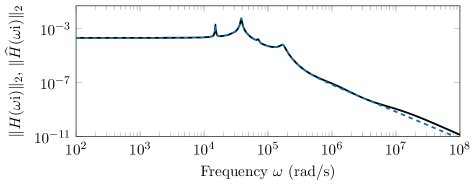
(a) Sigma plots.

graphics/butterfly_gyro_err.tikzgraphics/externalize/butterfly_gyro_err.pdf

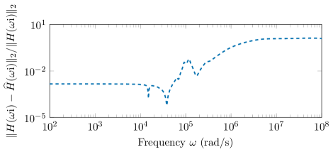
(b) Relative error.

graphics/butterfly_gyro_legend.tikzgraphics/externalize/butterfly_gyro_legend.pdf

Figure 1: Modally damped dominant pole algorithm results for the butterfly gyroscope example.

As an illustrative example, we consider the butterfly gyroscope benchmark from [39] with $n=17\,361$, $m=1$ and $p=12$. The used Rayleigh damping for the $D\leavevmode\nobreak\ (=10^{-6}\cdot K)$ matrix belongs to the class of modal damping. We are using the implementation from [21] to compute a reduced-order model with the first $10$ dominant pole pairs by the criterion Eq. 6. By construction, the resulting reduced-order model has order $10$. Figure 1 shows the results in the frequency domain with the frequency response behavior of the original and the reduced-order model and the pointwise relative error of the approximation. Up to a frequency of about $10^{6}$ rad/s, the behavior of the original system is well reproduced, while later, the two lines begin to diverge slightly. Additionally, Figure 2 shows the position of the computed dominant poles as projection onto the imaginary axis and the corresponding transfer function behavior.

Comparisons to other model reduction methods and further examples using this new dominant pole algorithm can be found in [51].

graphics/butterfly_gyro_pdp.tikzgraphics/externalize/butterfly_gyro_pdp.pdf

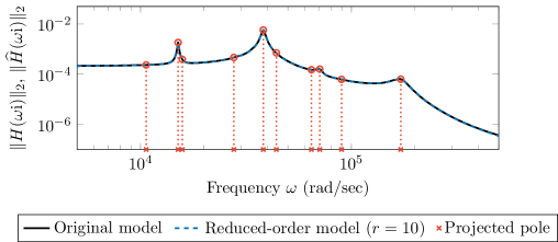
Figure 2: Projection of the computed dominant poles on the frequency axis compared with the transfer functions for the butterfly gyroscope example.

3 Second-order frequency- and time-limited balanced truncation

A global approximation of the system behavior in frequency or time domain is often not required in practice. The second-order limited balanced truncation approaches are a suitable tool for model order reduction restricted to certain frequency and time ranges. Thereby, the ideas from the first-order frequency- and time-limited balanced truncation methods [29] are combined with different second-order balanced truncation approaches [38, 23, 44]. A first version of these methods can be found in [6, 46, 33, 34] and the complete theory with applications to large-scale sparse systems is contained in [51, 18].

The idea of the method is based on the first companion form realization of Eq. 1, which is given by

$$\begin{aligned} \underbrace{\begin{bmatrix}I_{n}&0\\ 0&M\end{bmatrix}}_{\phantom{\,\mathcal{E}}=:\,\mathcal{E}}\dot{x}(t)&=\underbrace{\begin{bmatrix}0&I_{n}\\ -K&-D\end{bmatrix}}_{\phantom{\,\mathcal{A}}=:\,\mathcal{A}}x(t)+\underbrace{\begin{bmatrix}0\\ B_{\mathrm{u}}\end{bmatrix}}_{\phantom{\,\mathcal{B}}=:\,\mathcal{B}}u(t),\\ y(t)&=\underbrace{\begin{bmatrix}C_{\mathrm{p}}&C_{\mathrm{v}}\end{bmatrix}}_{\phantom{\,\mathcal{C}}=:\,\mathcal{C}}x(t).\end{aligned}$$ (7)

For Eq. 7, the classical controllability and observability Gramians are defined and can be limited as in [29]. Therefore, the frequency-limited Gramians $P_{\Omega}$ and $Q_{\Omega}$ of Eq. 7 are the unique symmetric positive semi-definite solutions of the potentially indefinite Lyapunov equations

$$\begin{aligned} \mathcal{A}P_{\Omega}\mathcal{E}^{\mkern-1.5mu\mathsf{T}}+\mathcal{E}P_{\Omega}\mathcal{A}^{\mkern-1.5mu\mathsf{T}}+\mathcal{B}_{\Omega}\mathcal{B}^{\mkern-1.5mu\mathsf{T}}+\mathcal{B}\mathcal{B}_{\Omega}^{\mkern-1.5mu\mathsf{T}}&=0,\\ \mathcal{A}^{\mkern-1.5mu\mathsf{T}}Q_{\Omega}\mathcal{E}+\mathcal{E}^{\mkern-1.5mu\mathsf{T}}Q_{\Omega}\mathcal{A}+\mathcal{C}_{\Omega}^{\mkern-1.5mu\mathsf{T}}\mathcal{C}+\mathcal{C}^{\mkern-1.5mu\mathsf{T}}\mathcal{C}_{\Omega}&=0,\end{aligned}$$

for a specified frequency range $\Omega=[\omega_{1},\omega_{2}]\cup[-\omega_{2},-\omega_{1}]$; see [29, 10]. The right-hand side matrices contain matrix functions, which are given by

$$\begin{aligned} \mathcal{B}_{\Omega}&=\left(\frac{\mathrm{i}}{\pi}\ln\left((\mathcal{A}+\omega_{2}\mathrm{i}\mathcal{E})(\mathcal{A}+\omega_{1}\mathrm{i}\mathcal{E})^{-1}\right)\right)\mathcal{B},\\ \mathcal{C}_{\Omega}&=\mathcal{C}\left(\frac{\mathrm{i}}{\pi}\ln\left((\mathcal{A}+\omega_{1}\mathrm{i}\mathcal{E})^{-1}(\mathcal{A}+\omega_{2}\mathrm{i}\mathcal{E})\right)\right).\end{aligned}$$

Analogously, the time-limited Gramians $P_{\Theta}$ and $Q_{\Theta}$ of Eq. 7 are given as the unique symmetric positive semi-definite solutions of the (potentially) indefinite Lyapunov equations

$$\begin{aligned} \mathcal{A}P_{\Theta}\mathcal{E}^{\mkern-1.5mu\mathsf{T}}+\mathcal{E}P_{\Theta}\mathcal{A}^{\mkern-1.5mu\mathsf{T}}+\mathcal{B}_{t_{0}}\mathcal{B}_{t_{0}}^{\mkern-1.5mu\mathsf{T}}-\mathcal{B}_{t_{\mathrm{f}}}\mathcal{B}_{t_{\mathrm{f}}}^{\mkern-1.5mu\mathsf{T}}&=0,\\ \mathcal{A}^{\mkern-1.5mu\mathsf{T}}Q_{\Theta}\mathcal{E}+\mathcal{E}^{\mkern-1.5mu\mathsf{T}}Q_{\Theta}\mathcal{A}+\mathcal{C}_{t_{0}}^{\mkern-1.5mu\mathsf{T}}\mathcal{C}_{t_{0}}-\mathcal{C}_{t_{\mathrm{f}}}^{\mkern-1.5mu\mathsf{T}}\mathcal{C}_{t_{\mathrm{f}}}&=0,\end{aligned}$$

where the time-dependent right-hand sides are defined as

$$\begin{aligned} \mathcal{B}_{t_{0}}&=\mathrm{e}^{\mathcal{A}\mathcal{E}^{-1}t_{0}}\mathcal{B},&\mathcal{B}_{t_{\mathrm{f}}}&=\mathrm{e}^{\mathcal{A}\mathcal{E}^{-1}t_{\mathrm{f}}}\mathcal{B},&\mathcal{C}_{t_{0}}&=\mathcal{C}\mathrm{e}^{\mathcal{E}^{-1}\mathcal{A}t_{0}},&\mathcal{C}_{t_{\mathrm{f}}}&=\mathcal{C}\mathrm{e}^{\mathcal{E}^{-1}\mathcal{A}t_{\mathrm{f}}}\end{aligned}$$

on the time interval $\Theta=[t_{0},t_{\mathrm{f}}]$; see [29, 36]. Using those Gramians for the different second-order balanced truncation approaches [38, 23, 44] leads to the second-order limited balanced truncation methods as described in [51, 18]. The dense version of the resulting methods is contained in the current version of the MORLAB toolbox [17, 19], and an implementation for large-scale sparse systems as MATLAB and GNU Octave toolbox can be found in [20].

graphics/triplechain_tf.tikzgraphics/externalize/triplechain_tf.pdf

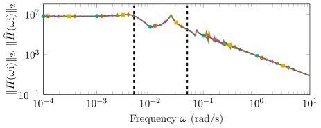
(a) Sigma plots.

graphics/triplechain_err.tikzgraphics/externalize/triplechain_err.pdf

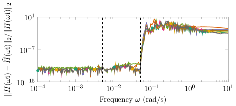
(b) Relative errors.

graphics/triplechain_legend.tikzgraphics/externalize/triplechain_legend.pdf

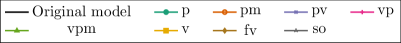
Figure 3: Frequency-limited balanced truncation results for the triple chain oscillator example.

As numerical example for the frequency-limited approach, we consider the triple chain oscillator example as in [6]. We reduce the original model ($n=1\,201$) by the second-order frequency-limited balanced truncation method in the interval $[5\cdot 10^{-3},5\cdot 10^{-2}]$ rad/s using the eight different second-order balancing formulas from [18] to the order $r=34$. The computations are done using the dense implementation of the second-order frequency-limited balanced truncation method from the latest version of the MORLAB toolbox [17, 19]. The results can be seen in Figure 3 with the transfer functions and the relative approximation errors. The computed reduced-order models are denoted according to the used balancing formulas from [18]. We clearly see the good approximation behavior in the frequency range of interest. Only the system computed by the fv formula is stable, while all others become unstable. The preservation of stability by the fv formula follows directly from the preservation of the symmetric positive definiteness of the system matrices via the underlying one-sided projection. However, note that in general for any balancing formula in the classical second-order balanced truncation method, there are counter-examples for the stability preservation [44].

graphics/singlechain_sim.tikzgraphics/externalize/singlechain_sim.pdf

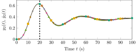
(a) Simulation outputs.

graphics/singlechain_err.tikzgraphics/externalize/singlechain_err.pdf

(b) Relative errors.

graphics/singlechain_legend.tikzgraphics/externalize/singlechain_legend.pdf

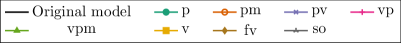
Figure 4: Time-limited balanced truncation results for the single chain oscillator example.

To illustrate the time-limited balanced truncation method, we use the single chain oscillator example as described in [18]. Here, we use the implementation for large-scale sparse mechanical systems from [20] to reduce the original system ($n=12\,000$) to order $r=3$ in the time interval $[0,20]$ s. The results for the second output entry can be seen in Figure 4, where in the time region of interest, the original system is nicely approximated by the reduced-order models. For all balancing formulas, the resulting systems are stable.

More detailed comparisons of the different balancing formulas and further examples can be found in [51, 18].

4 Positive real balanced truncation for second-order systems

In this section, we consider second-order systems of the form Eq. 1, where $M,K>0$, $D\geq 0$, and either we exclusively measure positions, i.e., $C_{\mathrm{v}}=0$, or velocities, i.e., $C_{\mathrm{p}}=0$. We start with the second case and additionally assume co-located inputs and outputs, which means $B_{\mathrm{u}}=C_{\mathrm{v}}^{\mkern-1.5mu\mathsf{T}}$. This case is treated in [27]. Using the Cholesky factorizations $K=GG^{\mkern-1.5mu\mathsf{T}}$ and $M=NN^{\mkern-1.5mu\mathsf{T}}$, the system can be rewritten in first-order form as

$$\begin{aligned} \dot{x}(t)&=\underbrace{\begin{bmatrix}0&G^{\mkern-1.5mu\mathsf{T}}N^{-\mkern-1.5mu\mathsf{T}}\\ -N^{-1}G&-N^{-1}DN^{-\mkern-1.5mu\mathsf{T}}\end{bmatrix}}_{\phantom{\,\mathcal{A}}=:\,\mathcal{A}}x(t)+\underbrace{\begin{bmatrix}0\\ N^{-1}B_{\mathrm{u}}\end{bmatrix}}_{\phantom{\,\mathcal{B}}=:\,\mathcal{B}}u(t),\\ y(t)&=\underbrace{\begin{bmatrix}0&B_{\mathrm{u}}^{\mkern-1.5mu\mathsf{T}}N^{-\mkern-1.5mu\mathsf{T}}\end{bmatrix}}_{\phantom{\,\mathcal{C}}=:\,\mathcal{C}}x(t).\end{aligned}$$ (8)

Besides passivity, the most important feature of this system is that it has an internal symmetry structure $\mathcal{A}\mathcal{S}_{n}=\mathcal{S}_{n}\mathcal{A}^{\mkern-1.5mu\mathsf{T}}$ and $\mathcal{C}=\mathcal{B}^{\mkern-1.5mu\mathsf{T}}=\mathcal{B}^{\mkern-1.5mu\mathsf{T}}\mathcal{S}_{n}$, where $\mathcal{S}_{n}:=\operatorname{diag}(-I_{n},I_{n})$. In particular, its transfer function $H(s)=\mathcal{C}(sI_{2n}-\mathcal{A})^{-1}\mathcal{B}$ is symmetric, i.e., it fulfills $H(s)^{\mkern-1.5mu\mathsf{T}}=H(s)$. We will make heavy use of this symmetry structure.

The model reduction technique consists of two steps:

Step 1: We apply positive real balanced truncation [32] to the first-order system Eq. 8. Here, the computational bottleneck is determining the numerical solution of the Lur’e equations

$$\begin{aligned} \mathcal{A}^{\mkern-1.5mu\mathsf{T}}P+P\mathcal{A}&=-K_{\mathrm{c}}^{\mkern-1.5mu\mathsf{T}}K_{\mathrm{c}},&\mathcal{A}Q+Q\mathcal{A}^{\mkern-1.5mu\mathsf{T}}&=-K_{\mathrm{o}}^{\mkern-1.5mu\mathsf{T}}K_{\mathrm{o}},\\ P\mathcal{B}-\mathcal{C}^{\mkern-1.5mu\mathsf{T}}&=0,&Q\mathcal{C}^{\mkern-1.5mu\mathsf{T}}-\mathcal{B}&=0,\end{aligned}$$

for stabilizing solutions $P,Q\in\mathbb{R}^{2n\times 2n}$; see [43]. The internal symmetry structure of Eq. 8 yields $Q=\mathcal{S}_{n}P\mathcal{S}_{n}$, hence only the Lur’e equation $\mathcal{A}^{\mkern-1.5mu\mathsf{T}}P+P\mathcal{A}=-K_{\mathrm{c}}^{\mkern-1.5mu\mathsf{T}}K_{\mathrm{c}}$, $P\mathcal{B}-\mathcal{C}^{\mkern-1.5mu\mathsf{T}}=0$ has to be solved for the matrices $P$ and $K_{\mathrm{c}}$. We can use the method from [41] to obtain a low-rank approximate solution $P\approx L^{\mkern-1.5mu\mathsf{T}}L$. The sign symmetry of the first-order system Eq. 8 yields that its positive real characteristic values (which are defined to be the positive square roots of the eigenvalues of $PQ$) can in a certain sense be allocated to the symmetry structure of the system Eq. 8. More precisely, the positive real characteristic values are the absolute values of the eigenvalues of the symmetric matrix $L\mathcal{S}_{n}L^{\mkern-1.5mu\mathsf{T}}$. By truncating equally many states corresponding to positive and negative eigenvalues of $L\mathcal{S}_{n}L^{\mkern-1.5mu\mathsf{T}}$, it is shown that the resulting first-order model is – without any further computational effort – of the form

$$\begin{aligned} \dot{\hat{x}}(t)&=\begin{bmatrix}0&0&0&0&0&\mathcal{A}_{16}\\ 0&0&0&0&\mathcal{A}_{25}&\mathcal{A}_{26}\\ 0&0&\mathcal{A}_{33}&\mathcal{A}_{34}&0&\mathcal{A}_{36}\\ 0&0&-\mathcal{A}_{34}^{\mkern-1.5mu\mathsf{T}}&\mathcal{A}_{44}&0&\mathcal{A}_{46}\\ 0&-\mathcal{A}_{25}^{\mkern-1.5mu\mathsf{T}}&0&0&0&0\\ -\mathcal{A}_{16}^{\mkern-1.5mu\mathsf{T}}&-\mathcal{A}_{26}^{\mkern-1.5mu\mathsf{T}}&-\mathcal{A}_{36}^{\mkern-1.5mu\mathsf{T}}&\mathcal{A}_{46}^{\mkern-1.5mu\mathsf{T}}&0&\mathcal{A}_{66}\end{bmatrix}{\hat{x}}(t)+\begin{bmatrix}0\\ 0\\ 0\\ 0\\ 0\\ \mathcal{B}_{6}\end{bmatrix}u(t),\\ \hat{y}(t)&=\begin{bmatrix}0&0&0&0&0&\mathcal{B}_{6}^{\mkern-1.5mu\mathsf{T}}\end{bmatrix}\hat{x}(t),\end{aligned}$$ (9)

where the block sizes from left to right and from top to bottom are $m,\ell,p,p,\ell,m$, with $r=p+m+\ell$. Note that, if $\mathcal{A}_{33}$ is zero, then – by merging some of the blocks – Eq. 9 has the form

$$\begin{aligned} \dot{\hat{x}}(t)&=\begin{bmatrix}0&\widehat{G}^{\mkern-1.5mu\mathsf{T}}\\ -\widehat{G}&-\widehat{D}\end{bmatrix}\hat{x}(t)+\begin{bmatrix}0\\ \widehat{B}_{\mathrm{u}}\end{bmatrix}u(t),\\ \hat{y}(t)&=\begin{bmatrix}0&\widehat{B}_{\mathrm{u}}^{\mkern-1.5mu\mathsf{T}}\end{bmatrix}\hat{x}(t),\end{aligned}$$ (10)

which results in a reduced-order model in second-order form Eq. 2 with $\widehat{M}=I_{r}$, $\widehat{K}=\widehat{G}\widehat{G}^{\mkern-1.5mu\mathsf{T}}$, $\widehat{C}_{\mathrm{p}}=0$, and $\widehat{C}_{\mathrm{v}}=\widehat{B}_{\mathrm{u}}^{\mkern-1.5mu\mathsf{T}}$. This is regrettably not the case in general, which is why we apply the following step.

Step 2: We apply a state-space transformation to Eq. 9 such that the matrix $\mathcal{A}_{33}$ vanishes. More precisely, we first intend to find some invertible $T\in\mathbb{R}^{2p\times 2p}$ that preserves the symmetry structure, i.e., it fulfills $T^{\mkern-1.5mu\mathsf{T}}\mathcal{S}_{p}T=\mathcal{S}_{p}$ and

$$T^{-1}\begin{bmatrix}\mathcal{A}_{33}&\mathcal{A}_{34}\\ -\mathcal{A}_{34}^{\mkern-1.5mu\mathsf{T}}&\mathcal{A}_{44}\end{bmatrix}T =\begin{bmatrix}0&\widehat{\mathcal{A}}_{34}\\ -\widehat{\mathcal{A}}_{34}^{\mkern-1.5mu\mathsf{T}}&\widehat{\mathcal{A}}_{44}\end{bmatrix}.$$

Then, a state-space transformation with $V=\operatorname{diag}(I_{m+\ell},T,I_{\ell+m})$ leads to a system which is indeed of the form Eq. 10 and can then be rewritten as a second-order system. Such a transformation is based on techniques from indefinite linear algebra [31], and can be computed without any remarkable computational effort. The existence of such a transformation is linked to the $2k$ real eigenvalues of $\begin{bmatrix}\mathcal{A}_{33}&\mathcal{A}_{34}\\ -\mathcal{A}_{34}^{\mkern-1.5mu\mathsf{T}}&\mathcal{A}_{44}\end{bmatrix}$. Under the assumption of semi-simplicity, these eigenvalues can be assigned a certain signature structure according to the sign of $-v_{i}^{\mkern-1.5mu\mathsf{T}}\mathcal{S}_{k}v_{i}$, where $v_{i}$ is the eigenvector of the $i$-th eigenvalue. In particular, we have $k$ eigenvalues $\mu_{1}^{-}\leq\ldots\leq\mu_{k}^{-}$ of negative type and $k$ eigenvalues $\mu_{1}^{+}\leq\ldots\leq\mu_{k}^{+}$ of positive type. It is then shown that such a transformation is possible, if $\mu_{i}^{-}<\mu_{i}^{+}$ for all $i=1,\ldots,k$. A sufficient criterion on the original system for the existence of such a transformation is that it is overdamped, that is $\big{(}v^{\mkern-1.5mu\mathsf{T}}Dv\big{)}^{2}>4\big{(}v^{\mkern-1.5mu\mathsf{T}}Mv\big{)}\big{(}v^{\mkern-1.5mu\mathsf{T}}Kv\big{)}$ for all $v\in\mathbb{R}^{n}$.

The resulting second-order system in particular fulfills $\widehat{M},\widehat{K}>0$, and it is further shown that $\widehat{D}=\widehat{D}^{\mkern-1.5mu\mathsf{T}}$ has at most $m$ negative eigenvalues. If the original system is overdamped, then even $\widehat{D}>0$. Moreover, the gap metric distance between the transfer functions $H(s)$ of the original and $\widehat{H}(s)$ of the reduced-order system is shown to be bounded from above by twice the sum of the truncated positive real characteristic values.

Considering a system dilation, we are able to extend the previously presented reduction to second-order systems with velocity measurements $y(t)=C_{\mathrm{p}}q(t)$, which are not necessarily co-located to the input. This can be done by considering the extended system

$$\begin{aligned} M\ddot{q}(t)+D\dot{q}(t)+Kq(t)&=\begin{bmatrix}B_{\mathrm{u}}&C_{\mathrm{v}}^{\mkern-1.5mu\mathsf{T}}\end{bmatrix}\begin{bmatrix}u_{1}(t)\\ u_{2}(t)\end{bmatrix},\\ \begin{bmatrix}y_{1}(t)\\ y_{2}(t)\end{bmatrix}&=\begin{bmatrix}B_{\mathrm{u}}^{\mkern-1.5mu\mathsf{T}}\\ C_{\mathrm{v}}\end{bmatrix}\dot{q}(t).\end{aligned}$$

This system is again positive real and from the algorithm above we thus obtain a reduced-order system for the extended system as

$$\begin{aligned} \widehat{M}\ddot{\hat{q}}(t)+\widehat{D}\dot{\hat{q}}(t)+\widehat{K}\hat{q}(t)&=\begin{bmatrix}\widehat{B}_{\mathrm{u}}&\widehat{C}_{\mathrm{v}}^{\mkern-1.5mu\mathsf{T}}\end{bmatrix}\begin{bmatrix}u_{1}(t)\\ u_{2}(t)\end{bmatrix},\\ \begin{bmatrix}\hat{y}_{1}(t)\\ \hat{y}_{2}(t)\end{bmatrix}&=\begin{bmatrix}\widehat{B}_{\mathrm{u}}^{\mkern-1.5mu\mathsf{T}}\\ \widehat{C}_{\mathrm{v}}\end{bmatrix}\dot{\hat{q}}(t),\end{aligned}$$ (11)

where $\widehat{B}_{\mathrm{u}}\in\mathbb{R}^{r\times m}$ and $\widehat{C}_{\mathrm{v}}\in\mathbb{R}^{p\times r}$. From that we obtain a reduced-order system for Eq. 1 as

$$\begin{aligned} \widehat{M}\ddot{\hat{q}}(t)+\widehat{D}\dot{\hat{q}}(t)+\widehat{K}\hat{q}(t)&=\widehat{B}_{\mathrm{u}}u_{1}(t),\\ \hat{y}_{2}(t)&=\widehat{C}_{\mathrm{v}}^{\mkern-1.5mu\mathsf{T}}\dot{\hat{q}}(t).\end{aligned}$$ (12)

As the transfer function of Eq. 12 is a submatrix of the transfer function of the system Eq. 11, and the same holds for the original system, the reduction error in the gap metric is bounded by the one of the extended system.

graphics/mass_spring_damper_3n_TruV09.tikzgraphics/externalize/mass_spring_damper_3n_TruV09.pdf

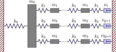
Figure 5: (3g + 1)-mass (triple chain) oscillator with three dampers [50].

We illustrate the performance of the reduction method above with an example of three coupled mass-spring-damper chains; see [50, Ex. 2]. The triple chain consists of three rows that are coupled via a mass $m_{0}$, which is connected to the fixed base with a spring with stiffness $k_{0}$. Each row contains $g$ masses, $g+1$ springs and one damper, which is attached to a wall; see Figure 5. One can write the free system as

$$M\ddot{q}(t)+D\dot{q}(t)+Kq(t) =0,$$

where $M,D$, and $K$ are defined as $M=\operatorname{diag}(m_{1},\ldots,m_{1},m_{2},\ldots,m_{2},\,m_{3},\ldots,m_{3})$, $D=\alpha M+\beta K+\nu_{1}e_{1}e_{1}^{\mkern-1.5mu\mathsf{T}}+\nu_{g+1}e_{g+1}e_{g+1}^{\mkern-1.5mu\mathsf{T}}+\nu_{2g+1}e_{2g+1}e_{2g+1}^{\mkern-1.5mu\mathsf{T}}$ and

$$\begin{aligned} K&=\begin{bmatrix}K_{11}&&&-\kappa_{1}\\ &K_{22}&&-\kappa_{2}\\ &&K_{33}&-\kappa_{3}\\ -\kappa_{1}^{\mkern-1.5mu\mathsf{T}}&-\kappa_{2}^{\mkern-1.5mu\mathsf{T}}&-\kappa_{3}^{\mkern-1.5mu\mathsf{T}}&\leavevmode\nobreak\ k_{1}+k_{2}+k_{3}+k_{0}\end{bmatrix},&K_{ii}&=k_{i}\begin{bmatrix}2&-1\\ -1&2&-1\\ &\ddots&\ddots&\ddots\\ &&-1&2&-1\\ &&&-1&2\end{bmatrix}\end{aligned}$$

with $\kappa_{i}=\begin{bmatrix}0&\ldots&0&k_{i}\end{bmatrix}^{\mkern-1.5mu\mathsf{T}}\in\mathbb{R}^{1\times g}$ and $K_{ii}\in\mathbb{R}^{g\times g}$ for $i=1,2,3$. We choose the input $B_{\mathrm{u}}=\begin{bmatrix}1&\ldots&1\end{bmatrix}^{\mkern-1.5mu\mathsf{T}}$ and equally measure the velocities such that $C_{\mathrm{v}}=B_{\mathrm{u}}^{\mkern-1.5mu\mathsf{T}}$. The second-order control system reads

$$\begin{aligned} M\ddot{q}(t)+D\dot{q}(t)+Kq(t)&=B_{\mathrm{u}}u(t),&y(t)&=B_{\mathrm{u}}^{\mkern-1.5mu\mathsf{T}}\dot{q}(t).\end{aligned}$$

We consider the triple chain with $g=500$, thus the number of differential equations is $n=3g+1=1\,501$. The stiffness and mass parameters are set as

$$\begin{aligned} k_{0}&=50,&k_{1}&=10,&k_{2}&=20,&k_{3}&=1,\\ m_{0}&=1,&m_{1}&=1,&m_{2}&=2,&m_{3}&=3,\end{aligned}$$

and the damping parameters $\alpha=\beta=0.002$ and $\nu_{1}=\nu_{g+1}=\nu_{2g+1}=5$.

Following the previously presented theory, we first compute a reduced-order model in first-order form of order $2r=200$ and then recover the structure of a second-order model of order $r=100$. The latter has again the form

$$\begin{aligned} \widehat{M}\ddot{\hat{q}}(t)+\widehat{D}\dot{\hat{q}}(t)+\widehat{K}\hat{q}(t)&=\widehat{B}_{\mathrm{u}}u(t),&\hat{y}(t)&=\widehat{B}_{\mathrm{u}}^{\mkern-1.5mu\mathsf{T}}\hat{q}(t),\end{aligned}$$

with symmetric $\widehat{M},\widehat{D},\widehat{K}\in\mathbb{R}^{r\times r}$ and $\widehat{B}_{\mathrm{u}}\in\mathbb{R}^{r\times m}$, where $\widehat{M}=I_{r}$, $\widehat{K}>0$ and $\widehat{D}=\widehat{D}^{\mkern-1.5mu\mathsf{T}}$. The plot of the absolute value of the original and reduced-order transfer functions can be found in Figure 6(a), whereas Figure 6(b) displays the relative error of the transfer function on the imaginary axis, respectively. With a maximum relative error of approximately $3.1\cdot 10^{-2}$ we obtain a good match between the original and the reduced-order system.

graphics/soprbt_systems.tikzgraphics/externalize/soprbt_systems.pdf

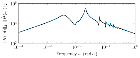
(a) Sigma plots.

graphics/soprbt_errorrel.tikzgraphics/externalize/soprbt_errorrel.pdf

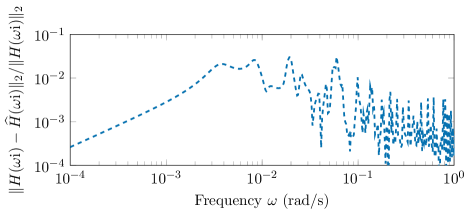
(b) Relative error.

graphics/soprbt_legend.tikzgraphics/externalize/soprbt_legend.pdf

Figure 6: Positive real balanced truncation results for the triple chain oscillator.

5 $\mathcal{H}_{\infty}$-optimal rational approximation

In this section, we briefly describe an interpolatory $\mathcal{H}_{\infty}$ model order reduction scheme for systems with symmetric mass, damping, and stiffness matrices and co-located inputs and position outputs, i.e., we have $M,D,K>0$, $B_{\mathrm{u}}=C_{\mathrm{p}}^{\mkern-1.5mu\mathsf{T}}$ and $C_{\mathrm{v}}=0$ in order to be able to preserve symmetry and asymptotic stability by an appropriate choice of the projection spaces. More precisely, we construct a sequence of reduced-order transfer functions of the form

$$\begin{aligned} \widehat{H}_{j}(s)&:=B_{\mathrm{u}}^{\mkern-1.5mu\mathsf{T}}V_{j}\big{(}s^{2}V_{j}^{\mkern-1.5mu\mathsf{T}}MV_{j}+sV_{j}^{\mkern-1.5mu\mathsf{T}}DV_{j}+V_{j}^{\mathsf{\mkern-1.5mu\mathsf{T}}}KV_{j}\big{)}^{-1}V_{j}^{\mkern-1.5mu\mathsf{T}}B_{\mathrm{u}},&j&=1,2,\ldots\end{aligned}$$

for appropriately chosen projection matrices $V_{j}$. Our method aims to iteratively reduce the $\mathcal{H}_{\infty}$-norm of the error transfer function $\mathcal{E}_{j}(s):=H(s)-\widehat{H}_{j}(s)$. To do so, we compute $\left\lVert\mathcal{E}_{j}\right\rVert_{\mathcal{H}_{\infty}}:=\max_{\omega\in\mathbb{R}\cup\{\infty\}}\left\lVert\mathcal{E}_{j}(\omega\mathrm{i})\right\rVert_{2}$. The point where $\left\lVert\mathcal{E}_{j}\right\rVert_{\mathcal{H}_{\infty}}$ is attained is denoted by $\omega_{j}\mathrm{i}$. We then choose $V_{j+1}:=\begin{bmatrix}V_{j}&(-\omega_{j}^{2}M+\omega_{j}\mathrm{i}D+K)^{-1}B_{\mathrm{u}}\end{bmatrix}$. For numerical reasons, $V_{j+1}$ (and all other projection matrices appearing in this section) are orthogonalized. This choice guarantees Hermite interpolation properties between the original and reduced-order transfer functions $H(s)$ and $\widehat{H}_{j}(s)$ at the interpolation points $\omega_{1}\mathrm{i}$, $\omega_{2}\mathrm{i}$, $\ldots$, $\omega_{j}\mathrm{i}$, such that the error near these points becomes small. This procedure is repeated until a specified error tolerance is met.

The main computational cost of this algorithm is the repeated computation of the $\mathcal{H}_{\infty}$-norm of the error transfer function, which is expensive to evaluate since the error system is of large dimension. However, these computations have been made possible by the methods presented in [1, 48], which we use here and which work as follows.

Assume that a transfer function is given by $H(s)=C(sE-A)^{-1}B$ with the regular matrix pencil $sE-A\in\mathbb{R}[s]^{n\times n}$, $B\in\mathbb{R}^{n\times m}$, and $C\in\mathbb{R}^{p\times n}$ with $n\gg m,p$. Then, the algorithm determines a sequence of reduced-order transfer functions of the form $H_{j}(s)=CV_{j}(sW_{j}^{\mathsf{H}}EV_{j}-W_{j}^{\mathsf{H}}AV_{j})^{-1}W_{j}^{\mathsf{H}}B$, where $V_{j},W_{j}\in\mathbb{C}^{n\times k_{j}}$ and $k_{j}\ll n$ for $j=1,2,\ldots,$ and where $\left\lVert H_{j}\right\rVert_{\mathcal{L}_{\infty}}:=\max_{\omega\in\mathbb{R}\cup\{\infty\}}\left\lVert H_{j}(\omega\mathrm{i})\right\rVert_{2}$ converges to $\left\lVert H\right\rVert_{\mathcal{H}_{\infty}}$. Since the matrices defining the reduced-order transfer functions $H_{j}(s)$, are of small dimensions, $\left\lVert H_{j}\right\rVert_{\mathcal{L}_{\infty}}$ can be efficiently computed using well-established methods such as [22, 16]. Assume first that $m=p$. Further suppose that $j$ interpolation points $\omega_{1}\mathrm{i},\ldots,\omega_{j}\mathrm{i}\in\mathrm{i}\mathbb{R}$ are already given. In this case, we choose

$$V_{j} =\begin{bmatrix}(\omega_{1}\mathrm{i}E-A)^{-1}B&\ldots&(\omega_{j}\mathrm{i}E-A)^{-1}B\end{bmatrix},$$

$$W_{j} =\begin{bmatrix}(\omega_{1}\mathrm{i}E-A)^{-\mathsf{H}}C^{\mathsf{H}}&\ldots&(\omega_{j}\mathrm{i}E-A)^{-\mathsf{H}}C^{\mathsf{H}}\end{bmatrix},$$

which amounts to the Hermite interpolation conditions

$$\begin{aligned} H(\omega_{k}\mathrm{i})&=H_{j}(\omega_{k}\mathrm{i}),&H^{\prime}(\omega_{k}\mathrm{i})&=H_{j}^{\prime}(\omega_{k}\mathrm{i}),&k&=1,\ldots,j,\end{aligned}$$

that carry over directly to the functions $\sigma(s):=\left\lVert H(s)\right\rVert_{2}$ and $\sigma_{j}(s):=\left\lVert H_{j}(s)\right\rVert_{2}$. These Hermite interpolation conditions are then used to prove a superlinear rate of convergence to a local maximum of $\sigma(\mathrm{i}\cdot)$ provided that the algorithm converges. The situation is more difficult if $m\neq p$ since then, $V_{j}$ and $W_{j}$ would have different dimensions and the pencil $sW_{j}^{\mathsf{H}}EV_{j}-W_{j}^{\mathsf{H}}AV_{j}$ would be singular. This situation also occurs if $V_{j}$ or $W_{j}$ do not have full column rank. Thus, an alternative choice for $V_{j}$ and $W_{j}$, which is outlined in [1], and QR factorizations can be used to obtain the matrices $V_{j},W_{j}$ such that the pencil $sW_{j}^{\mathsf{H}}EV_{j}-W_{j}^{\mathsf{H}}AV_{j}$ is regular.

graphics/hinf_interpol.tikzgraphics/externalize/hinf_interpol.pdf

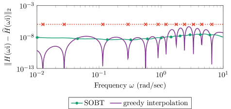
Figure 7: Comparison of absolute errors of different methods for second-order model reduction. The interpolation points of our greedy approach are plotted as red crosses.

In Figure 7, we illustrate the effectiveness of our algorithm using the triple chain oscillator benchmark example [50] (see Figure 5) of order $n=1\,000$ and an $\mathcal{H}_{\infty}$-error bound of $10^{-6}$. Compared with the second-order balanced truncation (SOBT, vp version) approach described in [44, Alg. 3.2], the greedy interpolation approach has a slightly larger maximal error for the same reduced order $r=29$. However, in contrast to SOBT, we obtain full information on the current error and may terminate whenever the reduced-order model satisfies a prescribed error bound. Moreover, the method also allows for an easy adaptation to frequency-limited reduction. We currently investigate post-processing strategies to improve the performance of the greedy interpolation such as an additional optimization of the interpolation points. Furthermore, our approach may be combined with the subspaces obtained from (SO)BT to initialize the first projection space.

The previously described algorithm leads to an error function $\mathcal{E}_{j}(s)$, which is zero at the interpolation points in exact arithmetics. This results in the spiky shape of the error maximum singular value function that can be observed in Figure 7. Such a behavior is generally unwanted, since this indicates that our reduced-order model approximates the given model at a few frequencies much better than at others. In this way, accuracy is “wasted” in a few regions that could be used to improve the overall accuracy of the reduced-order model. This is an inherent problem of a greedy approximation strategy with interpolation on the imaginary axis.

To smoothen the error maximum singular value function and reach a better approximation with respect to the $\mathcal{H}_{\infty}$-norm, we use direct numerical optimization. In particular, after a new interpolation point has been chosen according to the previously described greedy algorithm, we vary the interpolation points such that the $\mathcal{H}_{\infty}$-error is locally minimized. This requires the solution of a nonsmooth, nonconvex and nonlinear optimization problem. We use the method described in [24], implemented in the software package GRANSO. This iterative optimization requires the repeated evaluation of the $\mathcal{H}_{\infty}$-norm of the error system, which is high-dimensional. For that, we again apply the method described in [1], which is well-suited for this task.

It is important to note that the gradient of ${\lVert\mathcal{E}_{j}\rVert}_{\mathcal{H}_{\infty}}$ with respect to the interpolation points can be computed analytically. Furthermore, the direct optimization strategy is not limited to just the interpolation points. On top of that, we can optimize tangential directions of the interpolation as well. In case of tangential interpolation, the projection matrix can be chosen as

$$V_{j} =\begin{bmatrix}(s_{1}^{2}M+s_{1}D+K)^{-1}B_{\mathrm{u}}b_{1}&\ldots&(s_{j}^{2}M+s_{j}D+K)^{-1}B_{\mathrm{u}}b_{j}\end{bmatrix},$$

where $b_{k}\in\mathbb{C}^{m}$ and $s_{k}\in\mathbb{C}$ for $k=1,\dots,j$ are not in the spectrum of $s^{2}M+sD+K$. In this way, the interpolation condition is relaxed such that we now only have tangential Hermite interpolation between $H(s)$ and $\widehat{H}_{j}(s)$, that is

$$\begin{aligned} H(s_{k})b_{k}&=\widehat{H}_{j}(s_{k})b_{k},&b_{k}^{\mathsf{H}}H(s_{k})&=b_{k}^{\mathsf{H}}\widehat{H}_{j}(s_{k}),&b_{k}^{\mathsf{H}}H^{\prime}(s_{k})b_{k}&=b_{k}^{\mathsf{H}}\widehat{H}_{j}^{\prime}(s_{k})b_{k},\end{aligned}$$

for $k=1,\dots,j$. This results in an optimization that can exploit more degrees of freedom, while the size of the projection matrix and hence the size of the reduced-order model is further reduced.

graphics/hinf_errorplot2.tikzgraphics/externalize/hinf_errorplot2.pdf

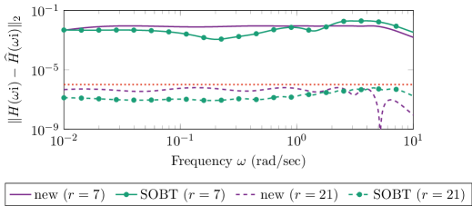
Figure 8: Comparison of the (absolute) errors of SOBT (vp) with the new, optimization-based method.

In Figure 8, we show a comparison of the errors between this new method and (the faster) SOBT on the triple chain oscillator example with $n=301$. The new method leads to an error function that is more steady and even outperforms the SOBT method for the smaller reduced-order model. However, for the slightly larger model order that is required to meet the given error bound of $10^{-6}$, the optimization got stuck in a local optimum and the error is less steady. Nevertheless, the accuracy is still comparable with the accuracy obtained by SOBT.

In order to improve the behavior of the error and make it globally more steady we have also recently developed a new optimization framework. There, we do not optimize the $\mathcal{H}_{\infty}$-error itself but rather parametrize the reduced-order model and then minimize the sum of squares of the error evaluated at certain sampling points on the imaginary axis [49].

6 Conclusions

We have presented an overview of recently developed structure-preserving model order reduction methods for second-order systems. We have started with an adaptation of the dominant pole algorithm for modally damped mechanical systems and, afterwards, have introduced extensions of the frequency- and time-limited balanced truncation methods for second-order systems in various ways. We have presented an approach for structure recovery of second-order systems based on positive real balanced truncation, which also yields an a priori error bound in the gap metric, and concluded with an $\mathcal{H}_{\infty}$ greedy interpolation approach yielding an $\mathcal{H}_{\infty}$-error optimal approximation. Numerical examples for all the presented approaches have illustrated their effectiveness.

Additionally to the approaches for linear systems summarized here, we were able to develop model order reduction techniques for (parametric) mechanical systems with special nonlinearities, namely bilinear control systems and quadratic-bilinear systems. These techniques are described in [51, 8, 9].

References

- [1] N. Aliyev, P. Benner, E. Mengi, P. Schwerdtner, and M. Voigt. Large-scale computation of -norms by a greedy subspace method. SIAM J. Matrix Anal. Appl., 38(4):1496–1516, 2017. doi:10.1137/16M1086200.
- [2] A. C. Antoulas. Approximation of Large-Scale Dynamical Systems, volume 6 of Adv. Des. Control. SIAM, Philadelphia, PA, 2005. doi:10.1137/1.9780898718713.
- [3] Z. Bai and Y. Su. Dimension reduction of large-scale second-order dynamical systems via a second-order Arnoldi method. SIAM J. Sci. Comput., 26(5):1692–1709, 2005. doi:10.1137/040605552.
- [4] C. Beattie and P. Benner. -optimality conditions for structured dynamical systems. Preprint MPIMD/14-18, Max Planck Institute for Dynamics of Complex Technical Systems Magdeburg, 2014. URL: https://csc.mpi-magdeburg.mpg.de/preprints/2014/18/.
- [5] C. A. Beattie and S. Gugercin. Interpolatory projection methods for structure-preserving model reduction. Syst. Control Lett., 58(3):225–232, 2009. doi:10.1016/j.sysconle.2008.10.016.
- [6] R. S. Beddig, P. Benner, I. Dorschky, T. Reis, P. Schwerdtner, M. Voigt, and S. W. R. Werner. Model reduction for second-order dynamical systems revisited. Proc. Appl. Math. Mech., 19(1):e201900224, 2019. doi:10.1002/pamm.201900224.
- [7] P. Benner, A. Cohen, M. Ohlberger, and K. Willcox. Model Reduction and Approximation: Theory and Algorithms. Computational Science & Engineering. SIAM, Philadelphia, PA, 2017. doi:10.1137/1.9781611974829.
- [8] P. Benner, S. Gugercin, and S. W. R. Werner. Structure-preserving interpolation for model reduction of parametric bilinear systems. Automatica J. IFAC, 132:109799, 2021. doi:10.1016/j.automatica.2021.109799.
- [9] P. Benner, S. Gugercin, and S. W. R. Werner. Structure-preserving interpolation of bilinear control systems. Adv. Comput. Math., 47(3):43, 2021. doi:10.1007/s10444-021-09863-w.
- [10] P. Benner, P. Kürschner, and J. Saak. Frequency-limited balanced truncation with low-rank approximations. SIAM J. Sci. Comput., 38(1):A471–A499, 2016. doi:10.1137/15M1030911.
- [11] P. Benner, P. Kürschner, and J. Saak. An improved numerical method for balanced truncation for symmetric second-order systems. Math. Comput. Model. Dyn. Syst., 19(6):593–615, 593–615. doi:10.1080/13873954.2013.794363.
- [12] P. Benner, P. Kürschner, Z. Tomljanović, and N. Truhar. Semi-active damping optimization of vibrational systems using the parametric dominant pole algorithm. ZAMM Z. Angew. Math. Mech., 96(5):604–619, 2016. doi:10.1002/zamm.201400158.
- [13] P. Benner, V. Mehrmann, and D. C. Sorensen. Dimension Reduction of Large-Scale Systems, volume 45 of Lect. Notes Comput. Sci. Eng. Springer, Berlin, Heidelberg, 2005. doi:10.1007/3-540-27909-1.
- [14] P. Benner and J. Saak. Efficient balancing-based MOR for large-scale second-order systems. Math. Comput. Model. Dyn. Syst., 17(2):123–143, 2011. doi:10.1080/13873954.2010.540822.
- [15] P. Benner, W. Schilders, S. Grivet-Talocia, A. Quarteroni, G. Rozza, and L. M. Silveira. Model Order Reduction. Volume 1: System- and Data-Driven Methods and Algorithms. De Gruyter, Berlin, Boston, 2021. doi:10.1515/9783110498967.
- [16] P. Benner, V. Sima, and M. Voigt. -norm computation for continuous-time descriptor systems using structured matrix pencils. IEEE Trans. Automat. Control, 57(1):233–238, 2012. doi:10.1109/TAC.2011.2161833.
- [17] P. Benner and S. W. R. Werner. MORLAB – Model Order Reduction LABoratory (version 5.0), August 2019. see also: https://www.mpi-magdeburg.mpg.de/projects/morlab. doi:10.5281/zenodo.3332716.
- [18] P. Benner and S. W. R. Werner. Frequency- and time-limited balanced truncation for large-scale second-order systems. Linear Algebra Appl., 623:68–103, 2021. Special issue in honor of P. Van Dooren, Edited by F. Dopico, D. Kressner, N. Mastronardi, V. Mehrmann, and R. Vandebril. doi:10.1016/j.laa.2020.06.024.
- [19] P. Benner and S. W. R. Werner. MORLAB—The Model Order Reduction LABoratory. In P. Benner, T. Breiten, H. Faßbender, M. Hinze, T. Stykel, and R. Zimmermann, editors, Model Reduction of Complex Dynamical Systems, volume 171 of International Series of Numerical Mathematics, pages 393–415. Birkhäuser, Cham, 2021. doi:10.1007/978-3-030-72983-7_19.
- [20] P. Benner and S. W. R. Werner. SOLBT – Limited balanced truncation for large-scale sparse second-order systems (version 3.0), April 2021. doi:10.5281/zenodo.4600763.
- [21] P. Benner and S. W. R. Werner. SOMDDPA – Second-Order Modally-Damped Dominant Pole Algorithm (version 2.0), April 2021. doi:10.5281/zenodo.3997649.
- [22] S. Boyd and V. Balakrishnan. A regularity result for the singular values of a transfer matrix and a quadratically convergent algorithm for computing its -norm. Systems Control Lett., 15(1):1–7, 1990. doi:10.1016/0167-6911(90)90037-U.
- [23] Y. Chahlaoui, D. Lemonnier, A. Vandendorpe, and P. Van Dooren. Second-order balanced truncation. Linear Algebra Appl., 415(2–3):373–384, 2006. doi:10.1016/j.laa.2004.03.032.
- [24] F. E. Curtis, T. Mitchell, and M. L. Overton. A BFGS-SQP method for nonsmooth, nonconvex, constrained optimization and its evaluation using relative minimization profiles. Optim. Methods Softw., 32(1):148–181, 2017. doi:10.1080/10556788.2016.1208749.
- [25] E. J. Davison. A method for simplifying linear dynamic systems. IEEE Trans. Automat. Control, 11(1):93–101, 1966. doi:10.1109/TAC.1966.1098264.
- [26] I. Dorschky. Balancing-Based Structure Preserving Model Order Reduction of Second Order Systems. Dissertation, Universität Hamburg, Germany, 2021. in print.
- [27] I. Dorschky, T. Reis, and M. Voigt. Balanced truncation model reduction for symmetric second order systems—A passivity-based approach. SIAM J. Matrix Anal. Appl., 42(4):1602–1635, 2021. doi:10.1137/20M1346109.
- [28] R. W. Freund. Padé-type model reduction of second-order and higher-order linear dynamical systems. In P. Benner, V. Mehrmann, and D. C. Sorensen, editors, Dimension Reduction of Large-Scale Systems, volume 45 of Lect. Notes Comput. Sci. Eng., pages 173–189. Springer, Berlin, Heidelberg, 2005. doi:10.1007/3-540-27909-1_8.
- [29] W. Gawronski and J.-N. Juang. Model reduction in limited time and frequency intervals. Int. J. Syst. Sci., 21(2):349–376, 1990. doi:10.1080/00207729008910366.
- [30] T. T. Georgiou and M. C. Smith. Optimal robustness in the gap metric. IEEE Trans. Automat. Control, 35(6):673–686, 1990. doi:10.1109/9.53546.
- [31] I. Gohberg, P. Lancaster, and L. Rodman. Matrices and Indefinite Scalar Products. Birkhäuser, Basel, Bosten, Stuttgart, 1983.
- [32] C. Guiver and M. R. Opmeer. Error bounds in the gap metric for dissipative balanced approximations. Linear Algebra Appl., 439(12):3659–3698, 2013. doi:10.1016/j.laa.2013.09.032.
- [33] K. Haider, A. Ghafoor, M. Imran, and F. M. Malik. Frequency interval Gramians based structure preserving model reduction for second-order systems. Asian J. Control, 20(2):790–801, 2018. doi:10.1002/asjc.1598.
- [34] K. Haider, A. Ghafoor, M. Imran, and F. M. Malik. Time-limited Gramian-based model order reduction for second-order form systems. Trans. Inst. Meas. Control, 41(8):2310–2318, 2019. doi:10.1177/0142331218798893.
- [35] C. Hartmann, V.-M. Vulcanov, and C. Schütte. Balanced truncation of linear second-order systems: A Hamiltonian approach. Multiscale Model. Simul., 8(4):1348–1367, 2010. doi:10.1137/080732717.
- [36] P. Kürschner. Balanced truncation model order reduction in limited time intervals for large systems. Adv. Comput. Math., 44(6):1821–1844, 2018. doi:10.1007/s10444-018-9608-6.
- [37] N. Martins, L. T. G. Lima, and H. J. C. P. Pinto. Computing dominant poles of power system transfer functions. IEEE Trans. Power Syst., 11(1):162–170, 1996. doi:10.1109/59.486093.
- [38] D. G. Meyer and S. Srinivasan. Balancing and model reduction for second-order form linear systems. IEEE Trans. Autom. Control, 41(11):1632–1644, 1996. doi:10.1109/9.544000.
- [39] Oberwolfach Benchmark Collection. Butterfly gyroscope. hosted at MORwiki – Model Order Reduction Wiki, 2004. URL: https://modelreduction.org/index.php/Butterfly_Gyroscope.
- [40] H. K. F. Panzer, T. Wolf, and B. Lohmann. and error bounds for model order reduction of second order systems by Krylov subspace methods. In Proceedings of the 2013 European Control Conference, pages 4484–4489, 2013. doi:10.23919/ECC.2013.6669657.
- [41] F. Poloni and T. Reis. A deflation approach for large-scale Lur’e equations. SIAM J. Matrix Anal. Appl., 33(4):1339–1368, 2012. doi:10.1137/120861679.
- [42] A. Quarteroni and G. Rozza. Reduced Order Methods for Modeling and Computational Reduction, volume 9 of MS&A – Modeling, Simulation and Applications. Springer, Cham, 2014. doi:10.1007/978-3-319-02090-7.
- [43] T. Reis. Lur’e equations and even matrix pencils. Linear Algebra Appl., 434(1):152–173, 2011. doi:10.1016/j.laa.2010.09.005.
- [44] T. Reis and T. Stykel. Balanced truncation model reduction of second-order systems. Math. Comput. Model. Dyn. Syst., 14(5):391–406, 2008. doi:10.1080/13873950701844170.
- [45] J. Rommes and N. Martins. Computing transfer function dominant poles of large-scale second-order dynamical systems. IEEE Trans. Power Syst., 21(4):1471–1483, 2006. doi:10.1109/TPWRS.2006.881154.
- [46] J. Saak, D. Siebelts, and S. W. R. Werner. A comparison of second-order model order reduction methods for an artificial fishtail. at-Automatisierungstechnik, 67(8):648–667, 2019. doi:10.1515/auto-2019-0027.
- [47] B. Salimbahrami and B. Lohmann. Order reduction of large scale second-order systems using Krylov subspace methods. Linear Algebra Appl., 415:385–405, 2006. doi:10.1016/j.laa.2004.12.013.
- [48] P. Schwerdtner and M. Voigt. Computation of the -norm using rational interpolation. IFAC-PapersOnline, 51(25):84–89, 2018. 9th IFAC Symposium on Robust Control Design ROCOND 2018, Florianópolis, Brazil. doi:10.1016/j.ifacol.2018.11.086.
- [49] P. Schwerdtner and M. Voigt. Structure preserving model order reduction by parameter optimization. e-print 2011.07567, arXiv, 2020. URL: https://arxiv.org/abs/2011.07567.
- [50] N. Truhar and K. Veselić. An efficient method for estimating the optimal dampers’ viscosity for linear vibrating systems using Lyapunov equation. SIAM J. Matrix Anal. Appl., 31(1):18–39, 2009. doi:10.1137/070683052.
- [51] S. W. R. Werner. Structure-Preserving Model Reduction for Mechanical Systems. Dissertation, Otto-von-Guericke-Universität, Magdeburg, Germany, 2021. doi:10.25673/38617.