Entropy-based test for generalized Gaussian distributions

Abstract

In this paper, we provide the proof of $L^{2}$ consistency for the $k$th nearest neighbour distance estimator of the Shannon entropy for an arbitrary fixed $k\geq 1.$ We construct the non-parametric test of goodness-of-fit for a class of introduced generalized multivariate Gaussian distributions based on a maximum entropy principle. The theoretical results are followed by numerical studies on simulated samples.

Keywords— Maximum entropy principle, generalized Gaussian distribution, Shannon entropy, nearest neighbour estimator of entropy, goodness-of-fit test.

1 Introduction

We propose a non-parametric test of goodness-of-fit for a class of generalized multivariate Gaussian distributions. Our approach is based on the estimation of the differential (Shannon) entropy

$$H(f)=-\int_{\mathbb{R}^{m}}f(x)\log f(x)\text{d}x$$ (1)

We use entropy estimators based on nearest neighbour distances. These were first studied by (Kozachenko & Leonenko, 1987) and subsequently by (Tsybakov & Van der Meulen, 1996; Evans et al., 2002; Goria et al., 2005; Leonenko et al., 2008; Leonenko & Pronzato, 2010; Evans, 2008; Penrose & Yukich, 2011; Delattre & Fournier, 2017; Gao et al., 2018; Bulinski & Dimitrov, 2019a, b) and Berrett et al. (2019). Nearest neighbour estimators (NNE) are particularly attractive because they are computationally efficient and generalise easily to the multivariate case. For an overview of non-parametric techniques of entropy estimation see Beirlant et al. (1997).

Berrett et al. (2019) have shown that subject to certain regularity conditions, as $k\to\infty$ the $k$-NNE of Shannon entropy is efficient only for $m\leq 3$, and present a bias-corrected estimator for dimensions $m\geq 4$. In this paper, we focus on the conventional $k$-NNE with fixed $k\geq 1$, for which the asymptotic variance decrease rapidly up to $k=3$ only, see (Berrett et al., 2019, Table 1). It is interesting to note that this asymptotic inflation is distribution-free, which leads to the conjecture that $k=3$ is the most interesting case for any $m\geq 1$.

Entropy-based tests of goodness-of-fit exploit the so-called maximum entropy principle Vasicek (1976); Kapur (1989). Choi (2008) introduced an entropy-based normality based on the fact that normal densities posses the largest Shannon entropy among all densities with the same variance, see also Dudewicz & Van Der Meulen (1981); Goria et al. (2005); Evans (2008) and the references therein. This paper proposes a new entropy-based test of generalized normality based on the maximum Shannon entropy principle for the generalized multivariate Gaussian distribution.

The paper is organised as follows: we introduce the multivariate generalized Gaussian distribution in section 3 followed by the $k$-NNE of Shannon entropy in section 2. In section 4 we establish a maximum entropy principle for the generalized Gaussian distribution, and in section 5 we present the associated goodness-of-fit statistics. Numerical results are included in section 6, with some auxiliary material deferred to Appendix A.

2 Entropy estimation

Let $k\geq 1$ and $N>k$, and let $\mathcal{X}_{N}=\{X_{1},\ldots,X_{N}\}$ be a set of independent and identically distributed random vectors in $\mathbb{R}^{m}$ with common density function $f$. Let $F$ be a finite subset of $\mathcal{X}_{N}$ having cardinality at least $k$, and let $\rho_{k}(x,F)$ denote the Euclidean distance between a point $x$ and its $k$th nearest neighbour in the set $F\setminus\{x\}$. The $k$th nearest neighbour estimator ($k$-NNE) of the Shannon entropy $H(f)$ is defined to be

$$\widehat{H}_{N,k} =\frac{1}{N}\sum_{i=1}^{N}\log\left[\rho_{k}^{m}(X_{i},\mathcal{X}_{N})V_{m}(N-1){e}^{-\psi(k)}\right],$$ (2)

where $\psi(x)=\Gamma^{\prime}(x)/\Gamma(x)$ is the digamma function and $V_{m}=\pi^{m/2}/\Gamma(m/2+1)$ is the volume of the unit ball in $\mathbb{R}^{m}$. For $k=1$, this reduces to

$$\widehat{H}_{N,1}=\frac{m}{N}\sum_{i=1}^{N}\log\rho_{1}(X_{i},\mathcal{X}_{N})+\log V_{m}+\gamma+\log(N-1).$$ (3)

where $\gamma=-\psi(1)\approx 0.577216$ is the Euler-Mascheroni constant. The estimator (3) was introduced by Kozachenko & Leonenko (1987) while the general estimator (2) was first considered by Goria et al. (2005). The main properties of (2) have been studied by Leonenko et al. (2008); Leonenko & Pronzato (2010); Penrose & Yukich (2011); Delattre & Fournier (2017); Gao et al. (2018); Bulinski & Dimitrov (2019a, b); Berrett et al. (2019) and Berrett & Samworth (2019).

Convergence in mean-square for the case $k=1$ was proved by (Penrose & Yukich, 2013, Theorem 2.1.ii).

Theorem 1 (Penrose & Yukich (2013)).

Suppose that $\mathbb{E}(\|X\|^{\alpha})<\infty$ for some $\alpha>0$ and $f(x)\leq M$ for some $M>0$. Then

$$\mathbb{E}\left[\widehat{H}_{N,1}-H(f)\right]^{2}\rightarrow 0\quad\text{as $N\to\infty$.}$$

Remark 1.

The condition of boundedness for the density $f$ is not explicitly stated by (Penrose & Yukich, 2013, Theorem 2.4.ii). In Appendix A we give an example of a density $f$ with bounded support and for which $H(f)$ is unbounded.

In this paper we prove the analogous result for arbitrary $k\geq 1$. To this end we write (2) as

$$\widehat{H}_{N,k}=\frac{1}{N}\sum_{x\in\mathcal{X}_{N}}l\left(N^{\frac{1}{m}}x,N^{\frac{1}{m}}\mathcal{X}_{N}\right),$$

where

$$l(x,\mathcal{X}):=\log\left(\rho_{k}^{m}(x,\mathcal{X})V_{m}e^{-\psi(k)}\right),x\in\mathbb{R}^{m}.$$

First, we require the following corollary of (Penrose & Yukich, 2013, Theorem 3.1).

Theorem 2.

Let $k\geq 1$ and $q=1$ or $q=2$, and suppose there exists $p\geq q$ such that

$$\sup_{N\geq k}\mathbb{E}\left|l\left(N^{\frac{1}{m}}X_{1},N^{\frac{1}{m}}\mathcal{X}_{N}\right)\right|^{p}<\infty.$$ (4)

Then we have $L^{q}$ convergence,

$$\frac{1}{N}\sum_{x\in\mathcal{X}_{N}}l\left(N^{\frac{1}{m}}x,N^{\frac{1}{m}}\mathcal{X}_{N}\right)\to\int_{\mathbb{R}^{m}}\mathbb{E}\left[l(0,\mathcal{P}_{f(x)})\right]f(x)\,dx,$$

as $N\to\infty$, where $\mathcal{P}_{\lambda}$ denotes a homogeneous Poisson point process of intensity $\lambda>0$ on $\mathbb{R}^{m}$.

Theorem 3 (Main theorem).

Suppose that $\mathbb{E}\|X\|^{\alpha}<\infty$ for some $\alpha>0$ and $f(x)\leq M$ for some $M>0$. Then for any fixed $k\geq 1$,

$$\mathbb{E}\left[\widehat{H}_{N,k}-H(f)\right]^{2}\to 0\quad\text{as $N\to\infty$.}$$ (5)

Proof.

We apply Theorem 2. First, we show that $H(f)=\displaystyle\int_{\mathbb{R}^{m}}\mathbb{E}\big{[}l(0,\mathcal{P}_{f(x)})\big{]}f(x)\,dx,$ where

$$l\left(0,\mathcal{P}_{\lambda}\right)=m\log\rho_{k}(0,\mathcal{P}_{\lambda})+\log V_{m}-\psi(k).$$

Denote by $B_{t}(0)$ the (Euclidean) ball of radius $t$ centred at $0$ i.e, $B_{t}(0)=\{y\in\mathbb{R}^{m},\|y\|\leq t\}.$ The random variable $\rho_{k}(0,\mathcal{P}_{\lambda})$ is the distance from $0$ to the $k$th point of $\mathcal{P}_{\lambda}$, and thus has Erlang distribution with parameters $k$ and $\lambda|B_{t}(0)|=\lambda V_{m}t^{m}$, that is

$$\mathbb{P}\big{(}\rho_{k}(0,\mathcal{P}_{\lambda})\leq t\big{)}=\mathbb{P}\big{(}\mathcal{P}_{\lambda}\cap B_{t}(0)\geq k\big{)}$$

$$=1-\sum_{j=0}^{k-1}\frac{1}{j!}\big{(}\lambda|B_{t}(0)|\big{)}^{j}e^{-\lambda|B_{t}(0)|}$$

$$=1-\sum_{j=0}^{k-1}\frac{1}{j!}(\lambda V_{m}t^{m})^{j}e^{-\lambda V_{m}t^{m}}\qquad(t\geq 0).$$

Then

$$m\mathbb{E}[\log\rho_{k}(0,\mathcal{P}_{\lambda})]$$

$$=\int_{0}^{\infty}\log t^{m}\frac{(\lambda V_{m})^{k}(t^{m})^{(k-1)}}{(k-1)!}e^{-\lambda V_{m}t^{m}}mt^{m-1}dt$$

$$=-\log(\lambda V_{m})+\int_{0}^{\infty}\log y\frac{y^{k-1}}{(k-1)!}e^{-y}dy$$

$$=-\log\lambda-\log V_{m}+\psi(k).$$

Hence $\mathbb{E}\big{[}l(0,\mathcal{P}_{\lambda})\big{]}=-\log\lambda$ and thus $H(f)$ equals

$$-\int_{\mathbb{R}^{m}}f(x)\log f(x)\,dx=\int_{\mathbb{R}^{m}}\mathbb{E}\big{[}l(0,\mathcal{P}_{f(x)})\big{]}f(x)\,dx.$$

Second, we check condition (4). Note that for every $\delta\in(0,1)$ and $p>1$ there exists $C>0$ such that

$$|\log t|^{p}\leq Ct^{-\delta}\mathbbm{1}_{[0,1]}(t)+Ct^{\delta}\mathbbm{1}_{[1,\infty)}(t),\qquad t>0.$$

Then because

$$|l(x,\mathcal{X})|^{p} =\big{|}\log V_{m}-\psi(k)+\log\rho_{k}^{m}(x,\mathcal{X})\big{|}^{p}$$

$$\leq\big{|}\log V_{m}-\psi(k)\big{|}^{p}+\big{|}\log\rho_{k}^{m}(x,\mathcal{X})\big{|}^{p}$$

we have

$$\frac{1}{2^{p-1}}\mathbb{E}\left|l\left(N^{\frac{1}{m}}X_{1},N^{\frac{1}{m}}\mathcal{X}_{N}\right)\right|^{p}$$

$$\leq\left|\log V_{m}-\psi(k)\right|^{p}+\mathbb{E}\left|\log\rho_{k}^{m}\left(N^{\frac{1}{m}}X_{1},N^{\frac{1}{m}}\mathcal{X}_{N}\right)\right|^{p}$$

$$\leq\left|\log V_{m}-\psi(k)\right|^{p}$$

$$+C\mathbb{E}\rho_{k}^{-\delta}\left(N^{\frac{1}{m}}X_{1},N^{\frac{1}{m}}\mathcal{X}_{N}\right)\mathbbm{1}_{[0,1]}\left[\rho_{k}^{\delta}\left(N^{\frac{1}{m}}X_{1},N^{\frac{1}{m}}\mathcal{X}_{N}\right)\right]$$ (6)

$$+C\mathbb{E}\rho_{k}^{\delta}\left(N^{\frac{1}{m}}X_{1},N^{\frac{1}{m}}\mathcal{X}_{N}\right)\mathbbm{1}_{[1,\infty)}\left[\rho_{k}^{\delta}\left(N^{\frac{1}{m}}X_{1},N^{\frac{1}{m}}\mathcal{X}_{N}\right)\right].$$ (7)

Term (6) is finite because

$$\sup_{N\geq k}\mathbb{E}\rho_{k}^{-\delta}\left(N^{\frac{1}{m}}X_{1},N^{\frac{1}{m}}\mathcal{X}_{N}\right)\mathbbm{1}_{[0,1]}\left(\rho_{k}^{\delta}\left(N^{\frac{1}{m}}X_{1},N^{\frac{1}{m}}\mathcal{X}_{N}\right)\right)$$

$$\leq\sup_{N\geq k}\mathbb{E}\rho_{1}^{-\delta}\left(N^{\frac{1}{m}}X_{1},N^{\frac{1}{m}}\mathcal{X}_{N}\right)<\infty,$$ (8)

where (8) is ensured by (Penrose & Yukich, 2013, Lemma 7.5) since $f$ is bounded and $\delta\in(0,m).$

Let $r_{c}(f):=\sup\{r\geq 0:\mathbb{E}\|X_{1}\|^{r}<\infty\}$. In the proof of (Penrose & Yukich, 2011, Theorem 2.3) we see that if $r_{c}(f)>0$ and $0<\delta<mr_{c}(f)(m+r_{c}(f))^{-1}$, then

$$\sup_{N\geq k}\mathbb{E}\rho_{k}^{\delta}\left(N^{\frac{1}{m}}X_{1},N^{\frac{1}{m}}\mathcal{X}_{N}\right)<\infty.$$

Thus, term (7) is finite.∎

3 The generalized Gaussian distribution

The multivariate exponential power distribution $\mathit{MEP}_{m}(s,\mu,\Sigma)$ on $\mathbb{R}^{m}$ Solaro (2004) has the density function

$$f(x\,;m,s,\mu,\Sigma)=\frac{\Gamma(m/2+1)}{\pi^{m/2}\Gamma(m/s+1)2^{m/s}\sqrt{\det\Sigma}}\exp\left(-\frac{1}{2}\Big{[}(x-\mu)^{\rm T}\Sigma^{-1}(x-\mu)\Big{]}^{s/2}\right)$$ (9)

where $\mu\in\mathbb{R}^{m}$ is the mean vector, $\Sigma$ is an $m\times m$ positive definite matrix, $s>0$ is a shape parameter Solaro (2004), and variance-covariance matrix $V=\beta\Sigma$ where

$$\beta(m,s)=\frac{2^{2/s}\Gamma\big{[}(m+2)/s\big{]}}{m\Gamma(m/s)}.$$ (10)

Note that $s=2$ corresponds to the multivariate normal distribution $N(\mu,\Sigma)$ on $\mathbb{R}^{m}$, while $s=1$ corresponds to the multivariate Laplace distribution. Taking $\mu$ to be the null vector and $\Sigma$ to be the identity matrix, we obtain the isotropic exponential power distribution $\mathit{IEP}_{m}(s)$ on $\mathbb{R}^{m}$,

$$f(x\,;m,s)=\frac{\Gamma(m/2+1)}{\Gamma(m/s+1)\pi^{m/2}2^{m/s}}\exp\left(-\frac{1}{2}\|x\|^{s}\right),$$ (11)

$x\in\mathbb{R}^{m},$ where $\|\cdot\|$ denotes the Euclidean norm on $\mathbb{R}^{m}$.

Applying the scaling $x\mapsto(2\tau)^{-1/s}x$ for $\tau>0$ yields the generalized Gaussian distributions $\mathit{GG}_{\tau}(m,s)$ on $\mathbb{R}^{m}$, with density functions

$$f_{c}(x;m,s)=c(m,s)\exp\left(-\tau\|x\|^{s}\right),x\in\mathbb{R}^{m},\\$$ (12)

where

$$\quad c(m,s)=\frac{\Gamma(m/2+1)\tau^{m/s}}{\Gamma(m/s+1)\pi^{m/2}},$$

and taking $\tau=1/s$ yields the canonical distribution

$$f(x;m,s)=c_{0}(m,s)\exp\left(-\frac{\|x\|^{s}}{s}\right),x\in\mathbb{R}^{m},$$ (13)

where

$$c_{0}(m,s)=\frac{\Gamma(m/2+1)}{\Gamma(m/s+1)\pi^{m/2}s^{m/s}}.$$

Moments

A random vector $X\in\mathbb{R}^{m}$ is called isotropic if its density $f$ can be written as $f(x)=\tilde{f}(\|x\|)$ for some function $\tilde{f}:\mathbb{R}\to[0,\infty)$ called the radial density, where $\|\cdot\|$ is the Euclidean norm on $\mathbb{R}^{m}$. If $X$ is isotropic and $g:\mathbb{R}\rightarrow\mathbb{R}$ is a Borel function, it is easy to show that

$$\mathbb{E}\left[g(\|X\|)\right]=\int_{\mathbb{R}^{m}}g(\|x\|)f(x)\,dx=\frac{2\pi^{m/2}}{\Gamma(m/2)}\int_{0}^{\infty}g(r)\tilde{f}(r)r^{m-1}\,dr$$ (14)

provided the integrals exist. In particular, the moments of order $s>0$ are given by

$$\mathbb{E}(\|X\|^{s})=\frac{2\pi^{m/2}}{\Gamma(m/2)}\int_{0}^{\infty}r^{m+s-1}\tilde{f}(r)\,dr$$ (15)

provided the integrals exist.

Lemma 1.

If $X\sim\mathit{GG}_{\tau}(m,s)$, then $\mathbb{E}(\|X\|^{s})=m/s\tau$.

Proof.

If $X\sim\mathit{GG}_{\tau}(m,s)$ then $X$ is isotropic and has radial density function

$$\tilde{f}(r)=\frac{\Gamma(m/2+1)\tau^{m/s}}{\Gamma(m/s+1)\pi^{m/2}}\exp(-\tau r^{s}).$$

Hence by (15) we have

$$\mathbb{E}(\|X\|^{s}) =\frac{2\pi^{m/2}}{\Gamma(m/2)}\int_{0}^{\infty}r^{s}\tilde{f}(r)r^{m-1}\,dr$$

$$=\frac{m\tau^{m/s}}{\Gamma(m/s+1)}\int_{0}^{\infty}r^{m+s-1}\exp(-\tau r^{s})\,dr$$

and changing the variable of integration to $t=\tau r^{s}$ yields

$$\mathbb{E}(\|X\|^{s}) =\frac{m}{s\tau\,\Gamma(m/s+1)}\int_{0}^{\infty}t^{m/s}e^{-t}dt=\frac{m}{s\tau}.$$

∎

4 A maximum entropy principle for $GG_{\tau}(m,s)$

It is well known Kapur (1989) that among all distributions on $\mathbb{R}^{m}$ whose densities $f$ are supported on the whole of $\mathbb{R}^{m}$ and whose mean and covariance matrix are fixed at zero and $\Sigma$ respectively, the differential entropy $H(f)$ is maximised by the multivariate Gaussian distribution $N(0,\Sigma)$ on $\mathbb{R}^{m}$, and thus

$$H(f)\leq\log\left[(2\pi e)^{m/2}\sqrt{\det\Sigma}\right].$$ (16)

We now prove an analogous result for the generalized Gaussian distribution.

Theorem 4.

Let $X\in\mathbb{R}^{m}$ be a random vector, whose density $f$ is supported on the whole of $\mathbb{R}^{m}$, and for which there exists some $s>0$ such that $\mathbb{E}(\|X\|^{s})<\infty$. Then $H(f)$ is finite and satisfies

$$H(f)\leq\frac{m}{s}\log\big{(}c_{1}(m,s)\mathbb{E}\|X\|^{s}\big{)},$$

where

$$c_{1}(m,s)=\left(\frac{\pi^{m/2}\Gamma(m/s+1)}{\Gamma(m/2+1)}\right)^{s/m}\left(\frac{se}{m}\right)$$

with equality if and only if $X\sim\mathit{GG}_{\tau}(m,s)$ with $\tau=m/(s\mathbb{E}\|X\|^{s})$.

Proof.

Let $X$ and $Z$ be two random vectors whose density functions, $f$ and $f^{*}$ respectively, are supported on the whole of $\mathbb{R}^{m}$, and for which there exists some $s>0$ with $\mathbb{E}\|X\|^{s}=\mathbb{E}\|Z\|^{s}<\infty$. First, we observe that

$$H(f)\leq-\int_{\mathbb{R}^{m}}f(x)\log f^{*}(x)\,dx,$$ (17)

with equality if and only if $f=f^{*}$ almost everywhere. This follows by Jensen’s inequality,

$$-\int_{\mathbb{R}^{m}}f(x)\log f(x)\,dx+\int_{\mathbb{R}^{m}}f(x)\log f^{*}(x)dx$$

$$=\int_{\mathbb{R}^{m}}f(x)\log\left(\frac{f^{*}(x)}{f(x)}\right)\,dx$$

$$\leq\log\left(\int_{\mathbb{R}^{m}}f(x)\left(\frac{f^{*}(x)}{f(x)}\right)\,dx\right)$$

$$=\log\left(\int_{\mathbb{R}^{m}}f^{*}(x)dx\right)=0.$$

If $Z\sim\mathit{GG}_{\tau}(m,s)$ with $\tau=\displaystyle\frac{m}{s\mathbb{E}\|X\|^{s}}$ (which ensures that $\mathbb{E}\|Z\|^{s}=\mathbb{E}\|X\|^{s}$) we have

$$f^{*}(x)=c(m,s)\exp(-\tau\|x\|^{s}),$$

where

$$c(m,s)=\frac{\Gamma(m/2+1)\tau^{m/s}}{\Gamma(m/s+1)\pi^{m/2}}.$$

For this case, $-\log f^{*}(x)=\tau\|x\|^{s}-\log c(m,s)$ and hence

$$-\int_{\mathbb{R}^{m}}f(x)\log f^{*}(x)dz$$

$$=\tau\int_{\mathbb{R}^{m}}\|x\|^{s}f(x)\,dx-(\log c(m,s))\int_{\mathbb{R}^{m}}f(x)\,dx$$

$$=\tau\,\mathbb{E}\|X\|^{s}-\log c(m,s)$$

$$=\frac{m}{s}-\log c(m,s)\quad\text{by Lemma~{}\ref{lem:moments-GG}.}$$

Thus by (17) and substituting for $c(m,s)$ we obtain

$$H(f) \leq\frac{m}{s}-\log\left[\frac{\tau^{m/s}\Gamma(m/2+1)}{\pi^{m/2}\Gamma(m/s+1)}\right]$$

$$=\frac{m}{s}\log\left[\left(\frac{\Gamma(m/s+1)}{\Gamma(m/2+1)}\right)^{\frac{s}{m}}\left(\frac{e\pi^{\frac{s}{2}}}{\tau}\right)\right],$$

and substituting for $\mathbb{E}\|X\|^{s}=m/(s\tau)$ completes the proof. ∎

Remark 2.

Theorem 4 was proved for $m=1$ in Wyner & Ziv (1969) and (Rosenblatt, 2000, p.103-104). For $m\geq 1$, some statements of Theorem 4 were also proved using other methods in Lutwak et al. (2007).

5 A test statistic for $GG(m,s)$

Let $k\geq 1$ be fixed and $\mathcal{K}$ be the class of density functions $f$ on $\mathbb{R}^{m}$ such that

1. $\mathrm{supp}(f)=\mathbb{R}^{m}$,

2. $\mathbb{E}(\|X\|^{s})<\infty$ for some $s>0$,

3. $\mathbb{E}(\widehat{H}_{N,k})\to H(f)$ as $N\to\infty$, and

4. $\widehat{H}_{N,k}\to H(f)$ in probability as $N\to\infty$.

Proposition 1.

The $\mathit{GG}_{\tau}(m,s)$ density functions belong to $\mathcal{K}$ for all $m\geq 1$, $s>0$, $c>0$ and $k\geq 1$.

Proof.

The statement follows from Theorem 3, which applies because $f$ is bounded, and Lemma 1. ∎

Let $X\in\mathbb{R}^{m}$ be a random vector with density $f\in\mathcal{K}$, and let $s>0$ be fixed. Based on a random sample $X_{1},X_{2},\dots$ from the distribution of $X$, we use the maximum entropy principle proved in Section 4 to test the hypothesis $X\sim\mathit{GG}(m,s)$ against a suitable alternative. By Theorem 4, if $X\sim\mathit{GG}(m,s)$ then

$$H(X)=\frac{m}{s}\log\mathbb{E}\|X\|^{s}+\frac{m}{s}\log c_{1}(m,s),$$

where

$$c_{1}(m,s)=\left(\frac{\pi^{m/2}\Gamma(m/s+1)}{\Gamma(m/2+1)}\right)^{s/m}\left(\frac{se}{m}\right).$$

We estimate the entropy $H(X)$ by the $k$th nearest neighbour estimator

$$\widehat{H}_{N,k}=\frac{m}{N}\sum_{i=1}^{N}\log\rho_{k}(X_{i},\mathcal{X}_{N})+\log V_{m}+\log(N-1)-\psi(k),$$

and the moment $\mathbb{E}\|X\|^{s}$ by the sample moment

$$\bar{X}^{(s)}_{N}=\frac{1}{N}\sum_{i=1}^{N}\|X_{i}\|^{s}.$$

Our test statistic $T_{N,k}=T_{N,k}(m,s)$ is then

$$T_{N,k} =\widehat{H}_{N,k}-\frac{m}{s}\log\bar{X}^{(s)}_{N}-\frac{m}{s}\log c_{1}(m,s).$$

By the law of a large numbers, $\bar{X}^{(s)}_{N}\to\mathbb{E}\|X\|^{s}$ in probability as $N\to\infty$. Hence by Slutsky’s theorem, if $X\sim\mathit{GG}_{m}(s)$ then for any fixed $k\in\{1,\ldots,N-1\}$ we have

$$T_{N,k}\to 0\quad\text{in probability as $N\to\infty$.}$$

Otherwise, by the maximum entropy principle it must be that $T_{N,k}\to\xi$ in probability as $N\to\infty$, where the constant $\xi=\xi(m,s,k)$ is strictly negative. Thus we reject the hypothesis $X\sim\mathit{GG}(m,s)$ whenever $T_{N,k}\geq t_{N,k,\alpha}$, where $t_{N,k,\alpha}=t_{N,k,\alpha}(m,s)$ a so-called critical value of the test statistic $T_{N,k}(m,s)$ at significance level $\alpha$, which is a solution of

$$\mathbb{P}_{H_{0}}\big{(}T_{N,k}\geq t\big{)}=\alpha.$$

An analytical derivation of the distribution of $T_{N,k}$ when $X\sim\mathit{GG}(m,s)$ is difficult because the covariances of $T_{N,k}$ and $\bar{X}^{(s)}_{N}$ are intractable, even though the asymptotic behaviour of $\widehat{H}_{N,k}$ can be revealed by applying results of Penrose & Yukich (2011); Delattre & Fournier (2017) or Berrett et al. (2019), and the asymptotic behaviour of $\bar{X}^{(s)}_{N}$ by the delta method. Thus we use Monte Carlo simulation to investigate the distribution of $T_{N,k}=T_{N,k}(m,s)$ for different combinations of parameter values.

Remark 3.

The test statistic $T_{N,k}$ is scale-invariant: if $Y=aX$ for some $a>0$, then $\widehat{H}_{N,k}(Y)=\log(a^{m})+\widehat{H}_{N,k}(X)$ and $\bar{Y}^{(s)}_{N}=a^{s}\bar{X}^{(s)}_{N}$, and hence

$$T_{N,k}(Y) =\widehat{H}_{N,k}(Y)-\frac{m}{s}\log\bar{Y}^{(s)}_{N}-\frac{m}{s}\log c_{1}(m,s)$$

$$=\log(a^{m})+\widehat{H}_{N,k}(X)-\frac{m}{s}\log(a^{s})$$

$$-\frac{m}{s}\log\bar{X}^{(s)}_{N}-\frac{m}{s}\log c_{1}(m,s)$$

$$=\widehat{H}_{N,k}(X)-\frac{m}{s}\log\bar{X}^{(s)}_{N}-\frac{m}{s}\log c_{1}(m,s)$$

$$=T_{N,k}(X).$$

6 Numerical results

To investigate the behaviour of $T_{N,k}(m,s)$ we generate random samples from the $\mathit{GG}(m,s)$ distribution, and also from the isotropic multivariate Student $t$-distribution $\mathit{ST}(m,\nu),$ $\nu>0$ on $\mathbb{R}^{m}$ which has density function

$$f(x;m,\nu)=\frac{\Gamma\big{[}(\nu+m)/2\big{]}}{\Gamma(\nu/2)(\nu\pi)^{m/2}}\left(1+\frac{\|x\|^{2}}{\nu}\right)^{-(\nu+m)/2},x\in\mathbb{R}^{m}.$$

This is achieved via the following stochastic representations Solaro (2004).

Lemma 2.

1. For $X\sim\mathit{GG}(m,s)$ we have $X\stackrel{{\scriptstyle d}}{{=}}UR$ where $U$ is uniformly distributed on $\mathbb{S}^{m-1}$ and $R\stackrel{{\scriptstyle d}}{{=}}V^{1/s}$ with $V\sim\text{Gamma}(m/s,2)$.

2. For $X\sim\mathit{ST}(m,\nu)$ we have $X\stackrel{{\scriptstyle d}}{{=}}Z/\sqrt{G}$, where $Z\sim N(0,I_{m})$ and $G\sim\text{Gamma}(\nu/2,2\nu)$.

For the case $m=2,$ we put the generated points on scatter plots for different values of $s$ and $\nu,$ see Figure 1 for $\mathit{GG}(m,s)$ and Figure 2 for $\mathit{ST}(m,\nu).$ One can observe that visually distributions $\mathit{GG}(m,s)$ and $\mathit{ST}(m,\nu)$ are hardly distinguishable. Therefore, we apply our goodness-of-fit test for detecting of the generalized Gaussian distribution.

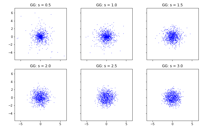
Figure 1: Scatter plots for $\mathit{GG}(m,s)$ with $m=2$

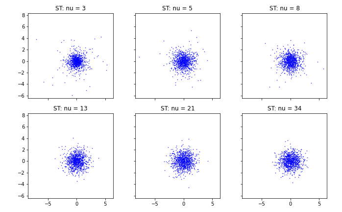
Figure 2: Scatter plots for $\mathit{ST}(m,\nu)$ with $m=2$

6.1 Empirical distribution of $\mathit{GG}(m,s)$

We generate $N=10^{6}$ points from the $\mathit{GG}(m,s)$ distribution for different values of $s$. For the purpose of comparison we apply the scaling $X\mapsto X/\sigma$ where

$$\sigma^{2}=\frac{2^{2/s}\Gamma\big{[}(m+2)/s\big{]}}{m\Gamma(m/s)}$$

is the variance of the $\mathit{GG}(m,s)$ distribution. The results are shown in Figure 3.

(a)

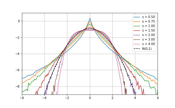
(b)

Figure 3: Empirical distribution of $\mathit{GG}(m,s)$ for $m=1$ and different values of $s$.

6.2 Asymptotic behaviour of $T_{N,k}(m,s)$ as $N\to\infty$.

For fixed $(N,k)$ and $(m,s)$ we generate a sample of size $N$ from the $\mathit{GG}(m,s)$ distribution and record the empirical value of $T_{N,k}(m,s)$, repeating this $M=10$ times. This yields a sample realisation $\{T_{1},T_{2},\ldots,T_{M}\}$ from the distribution of $T_{N,k}(m,s)$, from which we estimate its mean and variance by

$$\bar{T}_{N,k}=\frac{1}{M}\sum_{j=1}^{M}T_{i}\quad\text{and}\quad S^{2}_{N,k}=\frac{1}{M-1}\sum_{j=1}^{M}(T_{i}-\bar{T}_{N,k})^{2}$$

In Figures 4 and 5 we show how $\bar{T}_{N,k}(m,s)$ approaches 0 as $N$ increases for various values of $m$, $s$ and $k$. In Figure 6 we show its behaviour for $k=1$ with error bars corresponding to the standard error $S_{N,k}/\sqrt{M}$.

6.2.1 Asymptotic behaviour of $T_{N,k}(m,s_{0})$ on data from $GG(m,s_{1})$

For various values of $s_{0}$ and $s_{1}$ we generate samples from the $\mathit{GG}(m,s_{1})$ distribution and examine the behaviour of $T_{N,k}(m,s_{0})$ as $N$ increases. The results are shown in Figure 7 and Figure 8. When $s_{0}\neq s_{1}$ we see that the statistic approaches a strictly negative value, and that this becomes increasingly negative as the difference between $s_{0}$ and $s_{1}$ increases.

6.2.2 Asymptotic behaviour of $T_{N,k}(m,s)$ on data from $\mathit{ST}(m,\nu)$

For various values of $s$ we generate samples from the $\mathit{ST}(m,\nu)$ distribution and examine the behaviour of $T_{N,k}(m,s)$ as $N$ increases. The results are shown in Figure 9.

6.3 Empirical distribution of $T_{N,k}(m,s)$

Numerical results suggest that the distribution of $T_{N,k}(m,s)$ is asymptotically normal as the sample size $N\to\infty$. For different values of $(N,k)$ and $(m,s)$ we generate $N_{T}=1000$ samples from the $\mathit{GG}(m,s)$ distribution and record the corresponding values of $T_{N,k}(m,s)$, repeating this $M=10$ times. To each of these $10$ samples from the distribution of $T_{N,k}(m,s)$ we then apply the Shapiro-Wilk test for normality Shapiro & Wilk (1965) and record the $p$-value returned by the test.

Figure 10 shows how these $p$-values behave as $N$ increases, for various values of $m$, $s$ and $k$. The plots suggest that the normal hypothesis cannot be rejected for samples of size $N=200$ or more.

In Figure 11 we show how the $p$-values behave for $k=1$, with error bars corresponding to the standard error across the $M=10$ repetitions.

Appendix A Lower bound on Shannon entropy

Below we present some essentials about lower bounds of Shannon entropy. First, we show that there exist densities such that $-\infty=H(f)<\infty.$ We modify an example of (Gnedenko & Kolmogorov, 1954, p.223). For other examples, see Barron (1986).

Example 1.

Let $m=1$ and consider the density

$$f(x)=\left[x\log^{2}\frac{e}{x}\right]^{-1}\mathbbm{1}_{[0,1]}(x),\qquad x\in\mathbb{R}.$$ (18)

If $X$ is random variable with density $~{}\eqref{eq_1_dim}$, then for $s=1$

$$\mathbb{E}X=\mathbb{E}|X|=\int_{0}^{1}\left[\log^{2}\frac{e}{x}\right]^{-1}\text{d}x=1-\text{E}_{1}(1)\simeq 0.40365...,$$ (19)

where

$$\text{E}_{p}(z)=z^{p-1}\Gamma(1-p,z)=z^{p-1}\int_{z}^{\infty}\frac{e^{-zt}}{t^{p}}\text{d}t,\quad p>0,\quad z\geq 0,$$

is the generalized exponential integral. Thus by Theorem 4 with $m=1$ and $s=1$,

$$H(f)\leq\log\left[2e\mathbb{E}|X|\right]\simeq 0.8073.$$

From the other hand,

$$H(f)=-\int_{0}^{1}\left[x\log^{2}\frac{e}{x}\right]^{-1}\log\left[x\log^{2}\frac{e}{x}\right]^{-1}\text{d}x=-\infty.$$

Example 2.

For $m\geq 2,$ the similar properties has the density

$$f(x)=c_{2}(m)\left[\|x\|^{m}\log^{2}\frac{e}{\|x\|}\right]^{-1}\mathbbm{1}_{B_{1}(0)}(x),\quad x\in\mathbb{R}^{m},$$

where $c_{2}(m)=\Gamma(\frac{m}{2})/(2\pi^{m/2}).$ That is $f$ has finite moments but $H(f)=-\infty.$

If a random vector $X$ in $\mathbb{R}^{m}$ has a bounded density $f$ with $\|f\|_{\infty}=\sup_{x\in\mathbb{R}^{m}}f(x)<\infty$, then there is a lower bound for its entropy Bobkov & Madiman (2011))

$$\frac{1}{m}H(f)\geq\log\|f\|_{\infty}^{-1/m}.$$ (20)

If, in addition, $f$ is log-concave (that is, $\log f$ is concave), then

$$\log\|f\|_{\infty}^{-1/m}\leq\frac{1}{m}H(f)\leq 1+\log\|f\|_{\infty}^{-1/m}.$$

Moreover, provided the existence of $p$th moment $\|X\|_{p}=\left\{\mathbb{E}\|X\|^{p}\right\}^{1/p}<\infty$, $p\geq 1,$ one has for a log-concave density $f,$ see Marsiglietti & Kostina (2018),

$$H(f)\geq\log\frac{2\|X-\mathbb{E}[X]\|_{p}}{\left[\Gamma(1+p)\right]^{1/p}}.$$ (21)

If $m=1$, then for symmetric log-concave random variable

$$H(f)\geq\log\frac{2\|X\|_{p}}{\left[\Gamma(p+1)\right]^{1/p}},\quad p>-1.$$ (22)

If a symmetric log-concave random vector on $\mathbb{R}^{m}$ has finite second moments, then

$$H(f)\geq\frac{m}{2}\log\frac{(\det\Sigma_{x})^{1/m}}{c_{5}(m)},$$ (23)

where $\Sigma_{x}=\mathbb{E}\left[(X-\mathbb{E}X)(X-\mathbb{E}X)^{T}\right]$ denotes the the covariance matrix of $X$ and

$$c_{3}(m)=\frac{e^{2}m^{2}}{4\sqrt{2}(m+2)}.$$ (24)

Constant $c_{3}(m)$ can be improved in the case of unconditional random vectors. A function $f:\mathbb{R}^{m}\to\mathbb{R}^{m}$ is called unconditional if for every $(x_{1},\ldots,x_{m})\in\mathbb{R}^{m}$ and $(\varepsilon_{1},\ldots,\varepsilon_{m})\in\{-1,1\}^{m}$, one has

$$f(\varepsilon_{1}x_{1},\ldots,\varepsilon_{m}x_{m})=f(x_{1},\dots,x_{m}).$$

For example, the density of standard isotropic Gaussian vector is unconditional. Thus, if $X$ is unconditional, symmetric, and log-concave, then

$$c_{3}(m)=e^{2}/2.$$ (25)

The constant  (25) is better than the constant  (24) for $m\geq 5$.

Appendix B Monte-Carlo simulations

In this section, we illustrate the results of Monte-Carlo simulations by the series of Figures 4–11.

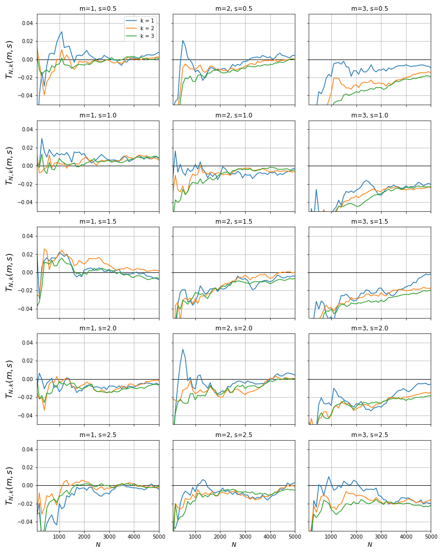
Figure 4: Consistency of $T_{N,k}(m,s)$ for different values of $k$ ($M=10$ repetitions).

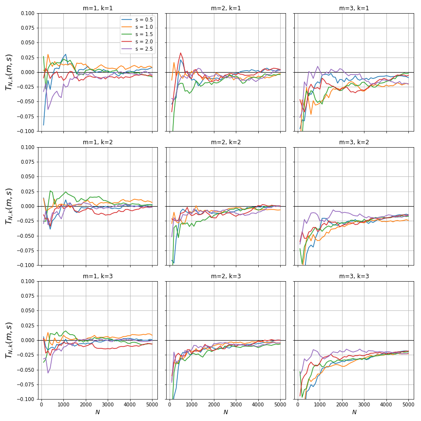
Figure 5: Consistency of $T_{N,k}(m,s)$ for different values of $s$ ($M=10$ repetitions).

Figure 6: Consistency of $T_{N,k}(m,s)$ for $k=1$ ($M=10$ repetitions).

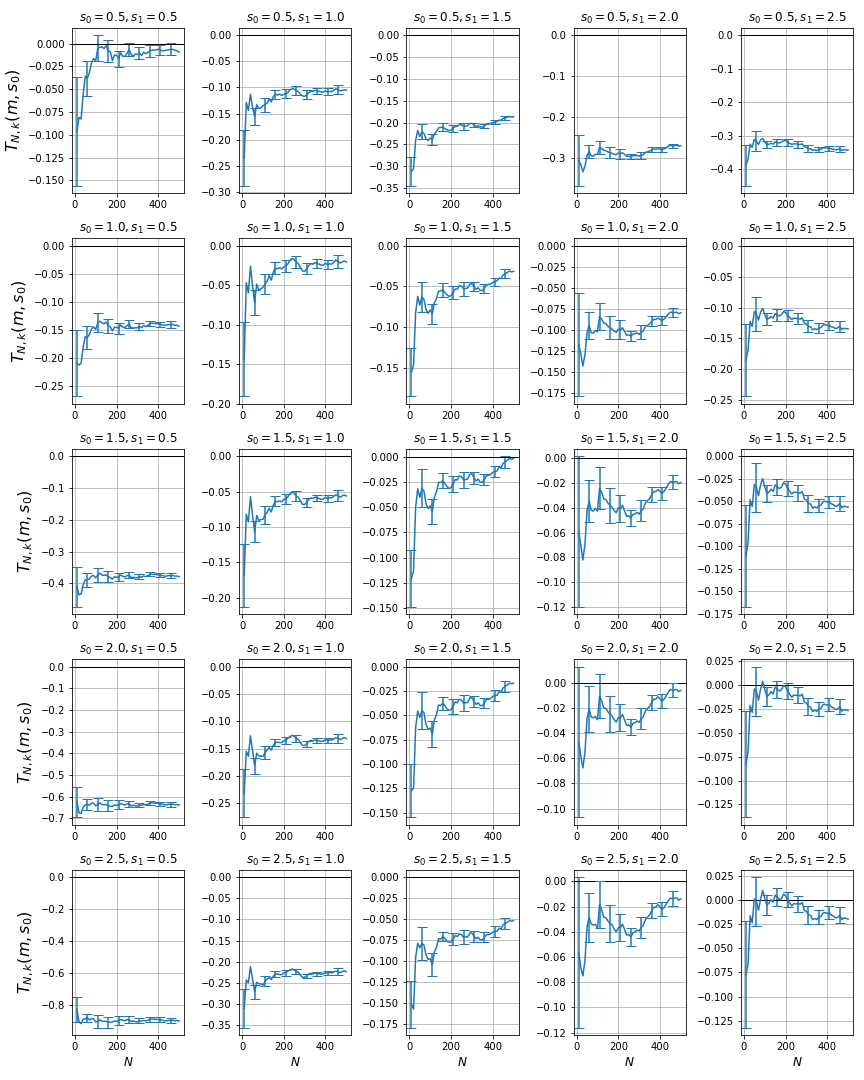
Figure 7: The behaviour of $T_{N,k}(m,s_{0})$ with $k=1$ on data from the $\mathit{GG}(m,s_{1})$ distribution with $m=2$.

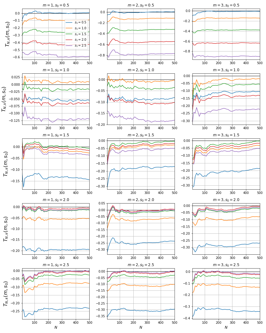
Figure 8: The behaviour of $T_{N,k}(m,s_{0})$ with $k=1$ on data from the $\mathit{GG}(m,s_{1})$ distribution for different values of $m$

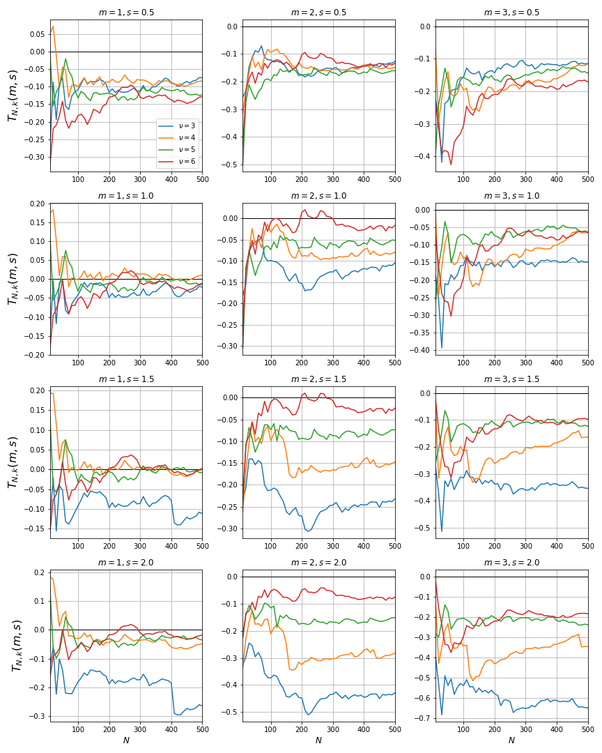
Figure 9: The behaviour of $T_{N,k}(m,s_{0})$ with $k=1$ on data from the $\mathit{ST}(m,\nu)$ distribution for different values of $m$.

Figure 10: Shapiro-Wilk $p$-values as $N$ increases for different values of $m$, $s$ and $k$ ($M=10$ repetitions).

Figure 11: Shapiro-Wilk $p$-values as $N$ increases for different values of $m$ and $s$ with $k=1$ ($M=10$ repetitions).

References

- Barron (1986) Barron, A. R. (1986). Entropy and the central limit theorem. Ann. Prob. 14, 336–342.
- Beirlant et al. (1997) Beirlant, J., Dudewicz, E. J., Györfi, L. & Van der Meulen, E. C. (1997). Nonparametric entropy estimation: An overview. International Journal of Mathematical and Statistical Sciences 6, 17–39.
- Berrett & Samworth (2019) Berrett, T. B. & Samworth, R. J. (2019). Nonparametric independence testing via mutual information. Biometrika 106, 547–566.
- Berrett et al. (2019) Berrett, T. B., Samworth, R. J. & Yuan, M. (2019). Efficient multivariate entropy estimation via -nearest neighbour distances. The Annals of Statistics 47, 288–318.
- Bobkov & Madiman (2011) Bobkov, S. & Madiman, M. (2011). The entropy per coordinate of a random vector is highly constrained under convexity conditions. IEEE Transactions on Information Theory 57, 4940–4954.
- Bulinski & Dimitrov (2019a) Bulinski, A. & Dimitrov, D. (2019a). Statistical estimation of the Kullback-Leibler divergence. arXiv preprint arXiv:1907.00196 .
- Bulinski & Dimitrov (2019b) Bulinski, A. & Dimitrov, D. (2019b). Statistical estimation of the Shannon entropy. Acta Mathematica Sinica, English Series 35, 17–46.
- Choi (2008) Choi, B. (2008). Improvement of goodness-of-fit test for normal distribution based on entropy and power comparison. Journal of Statistical Computation and Simulation 78, 781–788.
- Delattre & Fournier (2017) Delattre, S. & Fournier, N. (2017). On the Kozachenko–Leonenko entropy estimator. Journal of Statistical Planning and Inference 185, 69–93.
- Dudewicz & Van Der Meulen (1981) Dudewicz, E. J. & Van Der Meulen, E. C. (1981). Entropy-based tests of uniformity. Journal of the American Statistical Association 76, 967–974.
- Evans (2008) Evans, D. (2008). A computationally efficient estimator for mutual information. Proceedings of the Royal Society A: Mathematical, Physical and Engineering Sciences 464, 1203–1215.
- Evans et al. (2002) Evans, D., Jones, A. J. & Schmidt, W. M. (2002). Asymptotic moments of near–neighbour distance distributions. Proceedings of the Royal Society of London. Series A: Mathematical, Physical and Engineering Sciences 458, 2839–2849.
- Gao et al. (2018) Gao, W., Oh, S. & Viswanath, P. (2018). Demystifying fixed -nearest neighbor information estimators. IEEE Transactions on Information Theory 64, 5629–5661.
- Gnedenko & Kolmogorov (1954) Gnedenko, B. V. & Kolmogorov, A. N. (1954). Limit distributions for sums of independent random variables. Addison-Wesley Publishing Company, Inc., Cambridge, Mass.
- Goria et al. (2005) Goria, M. N., Leonenko, N. N., Mergel, V. V. & Novi Inverardi, P. L. (2005). A new class of random vector entropy estimators and its applications in testing statistical hypotheses. Journal of Nonparametric Statistics 17, 277–297.
- Kapur (1989) Kapur, J. N. (1989). Maximum-Entropy Models in Science and Engineering. John Wiley & Sons.
- Kozachenko & Leonenko (1987) Kozachenko, L. F. & Leonenko, N. N. (1987). Sample estimate of the entropy of a random vector. Problems of Information Transmission 23, 95–101.
- Leonenko & Pronzato (2010) Leonenko, N. N. & Pronzato, L. (2010). Correction: A class of Rényi information estimators for multidimensional densities. Annals of Statistics 38, 3837–3838.
- Leonenko et al. (2008) Leonenko, N. N., Pronzato, L. & Savani, V. (2008). A class of Rényi information estimators for multidimensional densities. The Annals of Statistics 36, 2153–2182.
- Lutwak et al. (2007) Lutwak, E., Yang, D. & Zhang, G. (2007). Moment-entropy inequalities for a random vector. IEEE Transactions on Information Theory 53, 1603–1607.
- Marsiglietti & Kostina (2018) Marsiglietti, A. & Kostina, V. (2018). A lower bound on the differential entropy of log-concave random vectors with applications. Entropy 20, 185.
- Penrose & Yukich (2011) Penrose, M. D. & Yukich, J. E. (2011). Laws of large numbers and nearest neighbor distances. In Advances in Directional and Linear Statistics. Springer, pp. 189–199.
- Penrose & Yukich (2013) Penrose, M. D. & Yukich, J. E. (2013). Limit theory for point processes in manifolds. The Annals of Applied Probability 23, 2161–2211.
- Rosenblatt (2000) Rosenblatt, M. (2000). Gaussian and Non-Gaussian Linear Time Series and Random Fields. Springer, New York.
- Shapiro & Wilk (1965) Shapiro, S. S. & Wilk, M. B. (1965). An analysis of variance test for normality (complete samples). Biometrika 52, 591–611.
- Solaro (2004) Solaro, N. (2004). Random variate generation from multivariate exponential power distribution. Statistica & Applicazioni 2, 25–44.
- Tsybakov & Van der Meulen (1996) Tsybakov, A. B. & Van der Meulen, E. (1996). Root-n consistent estimators of entropy for densities with unbounded support. Scandinavian Journal of Statistics , 75–83.
- Vasicek (1976) Vasicek, O. (1976). A test for normality based on sample entropy. Journal of the Royal Statistical Society: Series B (Methodological) 38, 54–59.
- Wyner & Ziv (1969) Wyner, A. D. & Ziv, J. (1969). On communication of analog data from a bounded source space. Bell System Technical Journal 48, 3139–3172.