Artist-driven layering and user’s behaviour impact on recommendations in a playlist continuation scenario

Abstract.

In this paper we provide an overview of the approach we used as team Creamy Fireflies for the ACM RecSys Challenge 2018. The competition, organized by Spotify, focuses on the problem of playlist continuation, that is suggesting which tracks the user may add to an existing playlist. The challenge addresses this issue in many use cases, from playlist cold start to playlists already composed by up to a hundred tracks. Our team proposes a solution based on a few well known models both content based and collaborative, whose predictions are aggregated via an ensembling step. Moreover by analyzing the underlying structure of the data, we propose a series of boosts to be applied on top of the final predictions and improve the recommendation quality. The proposed approach leverages well-known algorithms and is able to offer a high recommendation quality while requiring a limited amount of computational resources.

1. Introduction

Recommender systems are a useful tool to offer personalized and relevant content to users in many different sectors like e-commerce or entertainment, in such a way to help the user in identifying relevant content in a wide database. The ACM RecSys Challenge 2018 organized by Spotify focuses on automatic playlist continuation. This domain, as described in (Schedl et al., 2018), is characterized by two important issues that often arise in recommender systems: sparsity of the user-item interactions and the cold-start problem (Kaminskas and Ricci, 2012).

Collaborative Filtering (CF) (Koren and Bell, 2015) is one of the most successful and effective techniques available in recommender systems, however they are prone to rapidly loose their effectiveness when the user-item interactions are sparse. User-based CF considers users to be similar if they tend to interact with items in a similar way, while item-based CF considers tracks to be similar if many users interacted with them in a similar way. With increasing sparsity in the interactions, the ability of CF to accurately inference the similarity between playlists and tracks decreases.

Cold-start problem refers to the task of recommending items to new users and/or recommending new items to users. In case of an almost empty playlist, recommending tracks under the CF framework becomes difficult because there is not enough listening history to make robust recommendations. Also if a new track is added to the system and no user has previously listened to it, it is impossible to find other similar tracks.

In both of these cases Content-Based recommender systems alleviate the problem of recommendation by constructing item-item and user-user similarities from the features available for items and users, respectively (Aggarwal et al., 2016). Our team proposes a hybrid recommender system solution to the RecSys Challenge 2018 which merges collaborative filtering and content based techniques while leveraging at the same time both given playlists’ structure and domain knowledge. As per competition rules, the source code is publicly available .

The rest of the paper is organized as follows. In Section 2 we outline the problem formulation, the dataset structure and the evaluation metrics. In Section 3 we describe the preprocessing steps. In Section 4 we list the algorithms we have used. In Section 5 we describe the ensemble structure and in Section 6 the post-processing steps and boosts. Section 7 describes how we addressed the creative track and which data we used. Finally Section 8 lists the computational requirements for the various phases of our proposed solution.

2. PROBLEM FORMULATION

The RecSys Challenge focuses on the music recommendation task, in particular on automatic playlist continuation. The goal is to develop a recommender system which is able, given a playlist and some related information to generate a list of recommended tracks that can be added to that playlist, thereby ”continuing” it. The challenge is split in two parallel tracks with different rules:

• Main track: only the Million Playlist Dataset (MPD) can be used to train the recommender system.

• Creative track: external, public and freely available data sources are allowed in order to enrich the MPD and improve the quality of the recommendations.

2.1. Dataset description

Spotify provided for the competition two different datasets:

• The Million Playlist Dataset: contains $1M$ playlists created by users on the Spotify platform. These playlists were created between January 2010 and October 2017. Each playlist contains a title, the track list (including track metadata) editing information (last edit time, number of playlist edits) and other miscellaneous information about the playlist.

• The Challenge Set: contains $10K$ incomplete playlists. The challenge is to recommend 500 tracks for each of these playlists. Playlists are grouped into 10 different categories, with 1K playlists in each category:
  

  1. Playlists with title only

  2. Playlists with title and the first track

  3. Playlists with title and the first 5 tracks

  4. Playlists with first 5 tracks (no title)

  5. Playlists with title and the first 10 tracks

  6. Playlists with first ten tracks (no title)

  7. Playlists with title and the first 25 tracks

  8. Playlists with title and 25 random tracks

  9. Playlists with title and the first 100 tracks

  10. Playlists with title and 100 random tracks

For further details of the two datasets refer to the dataset website.

2.2. Evaluation metrics

Predictions are evaluated according to three different metrics and final rankings are computed using the Borda Count election strategy. Assuming the ground truth set of tracks defined by $G_{t}$, and the ordered list of recommended tracks by $R_{t}$:

• R-precision: this metric is evaluated both at the track level (e.g., tracks correctly recommended) and at the artist level (e.g., any other track by the same artist). The track level is computed as follows:

  $$Rprec_{t}=\frac{|G_{t}\cap R_{t_{1:|G_{t}|}}|}{|G_{t}|}$$

  Being $G_{a}$ the ground truth set of unique artists of $G_{t}$ and $R_{a}$ is the ordered list of recommended artists of $R_{t}$ for all the tracks which have not been matched at the track level, the artist level is computed as follows:

  $$Rprec_{a}=\frac{|G_{a}\cap R_{a}|}{|G_{a}|}$$

  A match at the artist level can only be counted once per artist per playlist. The final score is:

  $$Rprec=Rprec_{t}+0.25*Rprec_{a}$$

• NDCG: normalized discounted cumulative gain is a well known rank-based metric used in recommender system.

• Recommended Songs clicks: is computed as follows:

  $$clicks=\left\lfloor\frac{argmin_{i}\left\{R_{t_{i}}:R_{t_{i}}\in G_{t}\right\}-1}{10}\right\rfloor$$

  where $R_{t_{i}}$ is the track that occupies the $i$th index of the ordered list of recommended tracks $R_{t}$. Recommended Songs clicks is the number of refreshes needed before a relevant track is encountered.

3. PREPROCESSING

In order to address the cold-start problem in first category, where we have no available interactions for playlists, we apply information retrieval techniques to build a feature space from playlists titles. The following preprocessing steps have been adopted:

1. Removing spaces from titles made by only separated single letters.

2. Elimination of uncommon characters like dots and brackets.

3. Separation of words composed by letters and numbers, appending the resulting new tokens.

4. Appending to the title the Lancaster and Porter stemming of title’s words.

The result is a list that contains all the original tokens and the newly created ones.

3.1. Track position and Artist Heterogeneity

In this music recommendation domain playlists are created by users and sometimes exhibit a common underlying structure due to the way a user fills them.

1. Adding all the songs from the same Album one after another.

2. Creating playlists with tracks from only one Artist and the featurings that involve him.

3. Creating a long playlist of one genre and fill them in the years with new songs of the same artist.

4. Creating a playlist with many different artists in the first tracks, and readding the same artists later on as seen in Figure 1.

To leverage these patterns we define a new measure to estimate how diverse the artists are.

$$ArtistHeterogeneity_{p}=\log_{2}\left(\frac{\ \left|\ uniqueTracks_{p}\ \right|\ }{\ \left|\ uniqueArtists_{p}\ \right|\ }\right)$$

Where p is the playlist. A value of $ArH=0$ refers to a playlist with a lot a different artists, like the ones with the Top100 songs of a genre. A high value of $ArH$ points to a very repetitive playlist.

In particular, consider a set of 500 long playlists (from 100 to 250 songs). If you observe the first 20 songs or the same number of songs but sampled at random you will obtain very different values for ArtistHeterogeneity, see Figure 1. We are also able to exploit the behaviour highlighted by this results by applying both boosts and clustering, as it is described in Section 5.2 and 6.1

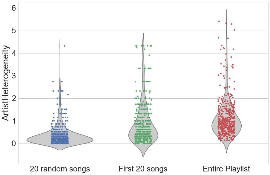
Figure 1. ArtistHeretogeneity for 1000 long playlists. The gray area behind the points shows the Distribution of ArH, over three different sampling strategies of songs in a long playlist.

4. ALGORITHMS

Our model is composed by five well known algorithms, some content based, some collaborative and some item-based and some user-based. In the following sections we will call playlist-track matrix (PTM) the matrix having the playlists as rows, tracks as columns and a cell value of one if the track belongs to that playlist.

4.1. Personalized Top Popular

For each element from category two, we implemented a personalized top popular algorithm based on the only track in the playlist.

4.1.1. Track Based

We select all the playlists containing that track and compute the top popular on them.

4.1.2. Album Based

Given the track’s album, we select all the playlists containing tracks from that album and compute the top popular on them.

4.2. Collaborative Filtering - Track Based

In the track-based CF algorithm first we apply BM25 (Robertson and Zaragoza, 2009) normalization on the PTM, then we define the similarity between two tracks i and j as the dot product between the corresponding PTM columns:

$$s_{ij}=r_{i}*r_{j}$$

The score prediction of target track i for playlist u is given by:

$$r_{ui}=\sum_{j\epsilon I(u)}^{KNN}r_{uj}*(s_{ji})^{p}$$

Where KNN are the top k-nearest neighbors and p is a coefficient that helps to discriminate values of the similarity.

4.3. Collaborative Filtering - Playlist Based

We define the similarity between two playlists i and j as the Tversky (Tversky, 1977) coefficient between the corresponding PCM rows:

$$s_{ij}=\frac{r_{i}*r_{j}}{\alpha(|r_{i}|-r_{i}*r_{j})+\beta(|r_{j}|-r_{i}*r_{j})+r_{i}*r_{j}+h}$$

Where $\alpha$ and $\beta$ are the Tversky coefficients between [0,1] and h is the shrink term.
The score prediction of target item i for user u is given by:

$$r_{ui}=\sum_{v\epsilon U(i)}^{KNN}(s_{uv})^{p}*r_{vi}$$

4.4. Content Based Filtering - Track Based

For the track-based content based filtering (CBF) we first applied BM25 normalization on the track-content matrix associating each track to its features, next we define the similarity between two tracks i and j as the dot product between the two feature vectors:

$$s_{ij}=f_{i}*f_{j}$$

The score prediction of target item i for user u is given by:

$$r_{ui}=\sum_{j\epsilon I(u)}^{KNN}r_{uj}*(s_{ji})^{p}$$

We run three different types of CBF, each one based on different combination of item features: Artist ID, Album ID, Album ID together with artist ID.

For the last one, after a phase of tuning, we assign different weight in the track content matrix giving more weight to the album features since it provides us better overall score.

4.5. Content Based Filtering - Playlist Based

We applied two different playlist-based CBF algorithms.

4.5.1. Track features

We build a playlist content matrix in which we represent playlists with the feature of the tracks they contain.

We then again built three different user-content matrix using different combinations of track features: Artist ID, Album ID, Album ID together with artist ID.

Next we apply BM25 on the playlist content matrix and we compute the similarity between two playlists i and j as the Tversky coefficient between the two playlist-feature vectors.

4.5.2. Playlist name

We create a playlist-content matrix for the tokens extracted from titles. Some playlists have untokenizable titles (e.g., emojis) to avoid empty recommendations and to improve accuracy we ensembled two different approaches relying on the playlist title

1. Content based filtering (CBF) based on the tokens extracted from the titles in the preprocessing phase.

2. Content based filtering (CBF) based on an exact title match.

The final model is a weighted sum of the recommendations of the two aforementioned approaches.

4.6. Parameters tuning

For each algorithm and for each category on which we are evaluated, we tune the parameters on our validation set.

• number of k-nearest neighbors (KNN) of the similarity matrices

• the power coefficient p for the similarity values

• the coefficients $\alpha$ and $\beta$ of the Tversky similarity

• the shrink term h

5. ENSEMBLE

5.1. Base Ensemble

An analysis on the case of study makes us observe that the different algorithms are better suited for subsets of playlists with specific characteristics. Content base approaches fit well on short playlists with similar features, on the other hand, collaborative filtering approaches gave us the best results on long and heterogeneous playlists.
We divide the results by category as it is shown in Figure 2. If we consider N algorithms, we use them to compute, for each playlist, N sets of tracks scores such that the highest valued tracks will be recommended to that playlist.

Figure 2. Category splitting of each algorithm.

The final model is a weighted sum of the N score predictions taking into account the length of the playlist and the position of the tracks. This allows to take advantage of the diversity in the predictions made by the different algorithms.

5.2. ArH-based Cluster Ensemble

One of the characteristics we took into account is the Artist Heterogeneity (ArH). Playlists are assigned to a cluster based on their ArH index, see Table 1.

	Cluster1	Cluster2	Cluster3	Cluster4
$ArH_{p}$	=0	¡1	¡2	¿=2

Table 1. Artist Heterogeneity clusters

For each category and for each cluster we search the best model weights by bayesian optimization, Figure 3.

Figure 3. Cluster division and Bayesian optimization

This ensemble also takes into account the cluster of the playlist. For the categories 4,5,6,8,10 this approach gives better results than the base ensemble (see Table 2). The final model for these categories is still a weighted sum of the N score predictions, but taking into account the ArH cluster.

	clicks	NDCG	R-precision
ArH-based	-0.0322	+0.0058	+0.0041

Table 2. Relative improvement for categories 4, 5, 6, 8, 10 after playlist’s clusterization.

6. POSTPROCESSING

Once we apply our per-category ensemble technique, we obtain a new set of predictions which takes into account the recommendations of each algorithm. We improve our score leveraging on domain-specific patterns of the dataset.

6.1. Boosts

The following boosts share a common work flow: they start from a list of $K$ predicted tracks for a playlist $p$ and for each $k\in K$ they boost the $Score_{p_{k}}$ computed via the ensemble model in this way:

$$Score_{p_{k}}=Score_{p_{k}}+Boost_{p_{k}}$$

6.1.1. Gap Boost

It is an heuristic which applies to playlists of category 8 and 10, where known tracks for each playlist are distributed at random. Since known tracks are not in order, there exist ”gaps” between each pair of known tracks. We exploit this information by reordering our final prediction giving more weight to tracks which seems to better ”fit” between all the gaps of the playlist. Therefore, for each playlist $p$ we select the first $K$ tracks of the prediction and we add to each of them the following value:

$$GapBoost_{p_{k}}=\gamma\sum_{g\in G}\frac{S_{k,g_{l}}\>S_{k,g_{r}}}{d_{g}}\quad\forall k\in K$$

where $S$ is a similarity matrix between tracks obtained by a content based filtering recommender as described in section 4.4, $G$ is the set of all the gaps in the playlist, $g_{l}$ and $g_{r}$ are the tracks which correspond respectively to the left boundary and the right boundary of the gap, $d_{g}$ is the length of the gap (the difference of the position in the playlist of the boundary tracks) and $\gamma$ is a weight factor. This technique improves significantly the R-precision and the Recommended clicks metrics, leaving the NDCG almost unchanged.

6.1.2. Tail Boost

We apply this technique to categories 5, 6, 7, 9, where known tracks for each playlist are given in order. The basic idea behind this approach is that the last tracks are the most informative about the ”continuation” of a playlist, therefore we boost all the top tracks similar to the last known tracks, starting from the tail and proceeding back to the head with a discount factor.

6.1.3. Album Boost

This approach leverages the fact that some playlists are built collecting tracks in order from a specific album. Therefore in categories 3, 4, 7 and 9, where known tracks for each playlist are given in order, we use this heuristic to boost all the tracks from a specific album where the last two known tracks belong to the same album. Album Boost improves the Recommender Songs clicks metric.

Algorithm	clicks	NDCG	R-precision
Gap Boost	-0.0003	+0.0001	+0.0021
Tail Boost	-0.0060	+0.0015	+0.0008
Album Boost	-0.0230	+0.0011	+0.0005

Table 3. Relative improvement of each boost on the three metrics.

7. Creative Track

Our approach to the creative track was heavily inspired by the approach used to compete in the main track. The rules of the competition specified that to qualify as successful, the final submission to the creative track must use external sources with the condition of being public and freely accessible to all participants.

7.1. External Datasets

Under the rules imposed by the competition organizers, we explored the datasets on table 4.

Dataset Name	Data Type	Year
#nowplaying music	Listening behavior	2018
#nowplaying playlists	Playlist	2015
MLHD	Listening behavior	2017
FMA	Audio Features	2017
MSD	Audio Features	2011
Spotify API	Audio Features, popularity	2018

Table 4. External datasets explored for the creative track. Listening behaviour refers to timestamps of listening events.

We spent considerable effort in trying to reconcile the tracks from the Million Playlist Dataset (MPD) provided by Spotify with those from external datasets but matching the name of the tracks and artists proved to be difficult and error-prone. Spotify Web API, on the other hand, being an API provided by Spotify itself, allowed us to retrieve for all tracks in MPD and in the Challenge Dataset the following features (using audio-features/{id} and tracks/{id} endpoints): acousticnes, danceability, energy, instrumentalness, liveness, loudness, speechiness, tempo, valence, popularity. During the data collection process, we found 159 tracks with missing audio features. As a preprocessing step, we filled in missing values for 159 tracks with the respective mean over all available data. For those tracks we are not able to retrieve popularity feature therefore we considered them as non-popular tracks, and filled in the missing values with 0, the lowest popularity level. In this way, we obtain a complete enriched dataset which contains 2,262,292 tracks and corresponding audio features and popularity.

7.2. Audio Feature Layered Content Based Filtering - Track Based

Inspired by the content based filtering (CBF) approach in the main track, we implemented a creative CBF which is able to adjust the artist based track recommendation using ten additional features from our enriched dataset.

In order to better illustrate the idea, we give a graphical representation of the item content matrix (ICM) by random sampling 200 artists.The track-track similarity matrix calculated with a normal CBF, as used in the main track, is not able to distinguish tracks belonging to the same artist. We call it artist-level similarity. This is clear if we take into consideration row $i$ of the ICM which represents a track; in $i$ only one column has a value of 1 corresponding to the artist of the track. For two tracks to be similar they must share the same artist thus making the similarity values of all $K$ most similar tracks to $i$ equal. In this way we cannot differentiate between similar tracks of i.

The creative CBF is implemented with the following steps:

1. Divide the tracks into 4 clusters with equal number of elements, according to each feature. Take the loudness feature as an example, the clustering result is shown in Figure 4.

2. Considering feature clusters as a 3rd dimension, split the dense ICM into 4 sparse layers. A loudness based layered ICM is illustrated in Figure 5.

3. Concatenate 4 layers of sparse matrices horizontally in order to create a final sparsified ICM.

4. Applying the CBF approach to the sparsified ICM, we can calculate a sub-artist-level track-track similarity.

In practice, this creative CBF is able to improve the artist-based recommendations in all three evaluation metrics. The comparison is presented on table 5 and 6.

Algorithm	clicks	NDCG	R-precision
CBF	19.9644	0.075191	0.037054
creative CBF	17.1286	0.086872	0.050467

Table 5. Track level local evaluation of artist based CBF and creative CBF (mean value of 10 categories)

Algorithm	clicks	NDCG	R-precision
CBF	17.4876	0.123445	0.003055
creative CBF	13.2587	0.159920	0.006016

Table 6. Artist level local evaluation of artist based CBF and creative CBF (mean value of 10 categories)

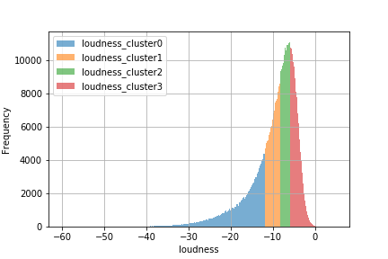
Figure 4. Clustering of tracks over loudness feature. The colors represent the different clusters.

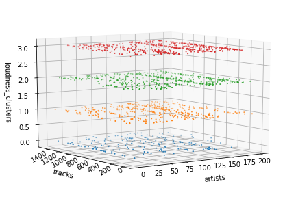
Figure 5. Layered ICM over loudness feature (200 sampled artists).

7.3. Feature Layered Collaborative Filtering - Track Based

Following the sparsifying idea in the previous subsection, we implement a layering procedure also to the playlist-track matrix. In creative track, the track features we used for layering procedure are: all feature clusters, album, artist. While in the main track, the layering idea is applied with only album and artist feature. Due to the different character of each category of playlists, in practice, we found out that this sparsified PTM has a good effect on the recommendation of the eighth and tenth category of playlists.

8. COMPUTATIONAL REQUIREMENTS

To run the entire model we use a AWS memory optimized cr1.8xlarge VM with 32 vCPU and 244 GiB of RAM.

Step	Time	RAM	Model dependent
Fast Models Creation 4	1h	150GB	Yes
Normal Models Creation 4	1.5h	80GB	Yes
Bayesian Optimization 5.2	16h	15GB	No
Ensemble 5	5m	¡8GB	Yes
Postprocessing 6.1	8m	¡8GB	Yes

Table 7. Computational requirements for the different steps. Model dependent steps need to be done again to recommend new playlists

The model creation can be done in two different ways depending on the needs and available resources.
The search of best parameters takes up to 16 hours on the appointed machine but is a procedure that needs to be computed only one time.

9. RESULTS AND CONCLUSION

Our recommendation architectures allowed us to reach the 4th place in the main track and the 2nd place in the creative track. The scores of our final model on both main and creative track are reported in Table 8. These scores are evaluated against 50 % of the challenge set, as stated in the website of the challenge. The predictions of most of the algorithms in the ensemble are heavily correlated. Nevertheless, the ensemble manages to extract the differing predictions from each algorithm, which is beneficial for the evaluation score. The major strength of our architecture is that is built in a simple and modular way. It can be easily extended with additional features coming from different datasets and new techniques can be implemented with no impact on the pre-existent work flow. Furthermore our architecture relies on an efficient Cython implementation of the most computationally intensive tasks, which allows to keep the time and space complexity under a reasonable threshold.

Track	clicks	NDCG	R-precision
Main	1.9810	0.3867	0.2207
Creative	1.9596	0.3858	0.2206

Table 8. Public Leaderboard scores of our final model on both main and creative track.

References

- (1)
- Aggarwal et al. (2016) Charu C Aggarwal et al. 2016. Recommender systems. Springer.
- Kaminskas and Ricci (2012) Marius Kaminskas and Francesco Ricci. 2012. Contextual music information retrieval and recommendation: State of the art and challenges. Computer Science Review 6, 2-3 (2012), 89–119.
- Koren and Bell (2015) Yehuda Koren and Robert Bell. 2015. Advances in collaborative filtering. In Recommender systems handbook. Springer, 77–118.
- Robertson and Zaragoza (2009) Stephen Robertson and Hugo Zaragoza. 2009. The Probabilistic Relevance Framework: BM25 and Beyond. Found. Trends Inf. Retr. 3, 4 (April 2009), 333–389. https://doi.org/10.1561/1500000019
- Schedl et al. (2018) Markus Schedl, Hamed Zamani, Ching-Wei Chen, Yashar Deldjoo, and Mehdi Elahi. 2018. Current challenges and visions in music recommender systems research. International Journal of Multimedia Information Retrieval 7, 2 (2018), 95–116.
- Tversky (1977) Amos Tversky. 1977. Features of Similarity. Psychological Review 84, 4 (1977), 327–352.