KLearn: Background Knowledge Inference from Summarization Data

Abstract

The goal of text summarization is to compress documents to the relevant information while excluding background information already known to the receiver. So far, summarization researchers have given considerably more attention to relevance than to background knowledge. In contrast, this work puts background knowledge in the foreground. Building on the realization that the choices made by human summarizers and annotators contain implicit information about their background knowledge, we develop and compare techniques for inferring background knowledge from summarization data. Based on this framework, we define summary scoring functions that explicitly model background knowledge, and show that these scoring functions fit human judgments significantly better than baselines. We illustrate some of the many potential applications of our framework. First, we provide insights into human information importance priors. Second, we demonstrate that averaging the background knowledge of multiple, potentially biased annotators or corpora greatly improves summary-scoring performance. Finally, we discuss potential applications of our framework beyond summarization.

1 Introduction

Summarization is the process of identifying the most important information pieces in a document. For humans, this process is heavily guided by background knowledge, which encompasses preconceptions about the task and priors about what kind of information is important Mani (1999).

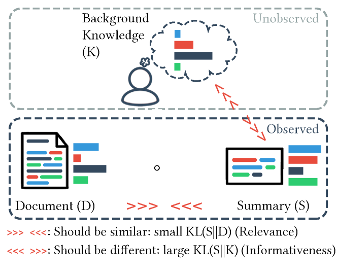
Figure 1: A summary ($S$) results from the combination of the background knowledge ($K$) and the source document ($D$). Following Peyrard (2019), $S$ is similar to $D$ (Relevance measured by a small $\textsc{{kl}}(S||D)$) but also brings new information compared to background knowledge (informativeness measured by a large $\textsc{{kl}}(S||K)$). We can infer the unobserved $K$ from the choices unexplained by the Relevance criteria.

Despite its fundamental role, background knowledge has received little attention from the summarization community. Existing approaches largely focus on the relevance aspect, which enforces similarity between the generated summaries and the source documents Peyrard (2019).

In previous work, background knowledge has usually been modeled by simple aggregation of large background corpora. For instance, using tf$\cdot$idf Sparck Jones (1972), one may operationalize background knowledge as the set of words with a large document frequency in background corpora.

However, the assumption that frequently discussed topics reflect what is, on average, known does not necessarily hold. For example, common-sense information is often not even discussed Liu and Singh (2004). Also, information present in background texts has already gone through the importance filter of humans, e.g., writers and publishers. In general, a particular difficulty preventing the development of proper background knowledge models is its latent nature. We can only hope to infer it from proxy signals. Besides, there is, at present, no principled way to compare and evaluate background knowledge models.

In this work, we put the background knowledge in the foreground and propose to infer it from summarization data. Indeed, choices made by human summarizers and human annotators provide implicit information about their background knowledge. We build upon a recent theoretical model of information selection Peyrard (2019), which postulates that information selected in the summary results from 3 desiderata: low redundancy (the summary contain diverse information), high relevance (the summary is representative of the document), and high informativeness (the summary adds new information on top of the background knowledge). The tension between these 3 elements is encoded in a summary scoring function $\theta_{K}$ that explicitly depends on the background knowledge $K$. As illustrated by Fig. 1, the latent $K$ can then be inferred from the residual differences in information selection that are not explained by relevance and redundancy. For example, the black information unit in Fig. 1 is not selected in the summary despite being very prominent in the source document. Intuitively, this is explained if this unit is already known by the receiver. To leverage this implicit signal, we view $K$ as a latent parameter learned to best fit the observed summarization data.

Contributions. We develop algorithms for inferring $K$ in two settings: (i) when only pairs of documents and reference summaries pairs are observed (Sec. 4.1) and (ii) when pairs of document and summaries are enriched with human judgments (Sec. 4.2).

In Sec. 5 we evaluate our inferred $K$s with respect to how well the induced scoring function $\theta_{K}$ correlates with human judgments. Our proposed algorithms significantly surpass previous baselines by large margins.

In Sec. 6, we give a geometrical perpespective on the framework and show that a clear geometrical structure emerges from real summarization data.

The ability to infer interpretable importance priors in a data-driven way has many applications, some of which we explore in Sec. 7. Sec. 7.1 qualitatively reveals which topics emerge as known and unkown in the fitted priors. Moreover, we can infer $K$ based on different subsets of the data. By training on the data of one annotator, we get a prior specific to this annotator. Similarly, one can find domain-specific $K$’s by training on different datasets. This is explored in Sec. 7.2, where we analyze $16$ annotators and $15$ different summarization datasets, yielding interesting insights, e.g., averaging several, potentially biased, annotator-specific or domain-specific $K$’s results in systematic generalization gains.

Finally, we discuss future work and potential applications beyond summarization in Sec. 8. Our code is available at https://github.com/epfl-dlab/KLearn

2 Related work

The modeling of background knowledge has received little attention by the summarization community, although the problem of identifying content words was already encountered in some of the earliest work on summarization Luhn (1958). A simple and effective solution came from the field of information retrieval, using techniques such as tf·idf on background corpora Sparck Jones (1972). Similarly, Dunning (1993) proposed the log-likelihood ratio test to identify highly descriptive words. These techniques are known to be useful for news summarization Harabagiu and Lacatusu (2005). Later approaches include heuristics to identify summary-worthy bigrams Riedhammer et al. (2010). Also, Hong and Nenkova (2014) proposed a supervised model for predicting whether a word will appear in a summary or not (using a large set of features including global indicators from the New York Times corpus) which can then serve as a prior of word importance.

Conroy et al. (2006) proposed to model background knowledge by aggregating a large random set of news articles. Delort and Alfonseca (2012) used Bayesian topic models to ensure the extraction of informative summaries. Finally, Louis (2014) investigated background knowledge for update summarization with Bayesian surprise.

These ideas have been generalized in an abstract model of importance Peyrard (2019) discussed in the next section.

3 Background

This work builds upon the abstract model introduced by Peyrard (2019), whose relevant aspects we briefly present here.

Let $T$ be a text and a function mapping a text to its semantic representation of the following form:

$$\{\mathbb{P}_{T}(\omega_{1}),\dots,\mathbb{P}_{T}(\omega_{n})\}$$ (1)

The semantic representation is a probability distribution $\mathbb{P}$ over so-called semantic units $\{\omega_{j}\}_{j\leq n}$. Many different text representation techniques can be chosen, e.g., topic models with topics as semantic units, or a properly renormalized semantic vector space with the dimensions as semantic units.

In the summarization setting, the source document $D$ and the summary $S$ are represented by probability distributions over the semantic units, $\mathbb{P}_{D}$ and $\mathbb{P}_{S}$. Similarly, $K$, the background knowledge, is represented as a distribution $\mathbb{P}_{K}$ over semantic units. Intuitively, $\mathbb{P}_{K}(\omega_{j})$ is high whenever $\omega_{j}$ is known. A summary scoring $\theta_{K}(S,D)$ (or simply $\theta_{K}(S)$ since the document $D$ is never ambiguous) can be derived from simple requirements:

$$\theta_{K}(S) =-\textsc{{red}}(S)+\alpha\cdot\textsc{{rel}}(S,D)+\beta\cdot\textsc{{inf}}(S,K)$$

$$=\textsc{{h}}(S)-\alpha\cdot\textsc{{kl}}(S\|D)+\beta\cdot\textsc{{kl}}(S\|K),$$ (2)

where red captures the redundancy in the summary via the entropy h. rel reflects the relevance of the summary via the Kullback-Leibler (KL) divergence between the summary and the document. A good summary is expected to be similar to the original document, i.e., the KL divergence $\textsc{{kl}}(S\|D)$ should be low. Finally, inf models the informativeness of the summary via the KL divergence between the summary and the latent background knowledge $K$. The summary should bring new information, i.e., the KL divergence $\textsc{{kl}}(S\|K)$ should be high.

In this work, we fix $\alpha=\beta=1$.

4 The KLearn framework

As laid out, in our framework, texts are viewed as distributions over a choice of semantic units $\{\omega_{j}\}_{j\leq n}$. We aim to infer a general $K$ as the distribution over these units that best explains summarization data. We consider two types of data: with and without human judgments.

4.1 Inferring $K$ without human judgments

Assume we have access to a dataset $\{x_{i}\}$ of pairs of documents $D_{i}$ and their associated summaries $S_{i}$: $x_{i}=(D_{i},S_{i})$. Under the assumption that the $S_{i}$ are good summaries (e.g., generated by humans), we infer the background knowledge $K$ that best explains the observation of these summaries. Indeed, if these summaries are good, we assume that information has been selected to minimize redundancy, maximize relevance and maximize informativeness.

Direct score maximization. A straightforward approach is to determine the $K$ that maximizes the $\theta_{K}$ score of the observed summaries. Formally, this corresponds to maximizing the function:

$$\mathcal{F}_{MS}(K)=\left[\sum\limits_{x_{i}}\theta_{K}(x_{i})\right]-\gamma\cdot\textsc{{kl}}(P\|K),$$ (3)

where $\textsc{{kl}}(P\|K)$ acts as a regularization term forcing $K$ to remain similar to a predefined distribution $P$. Here, $P$ can serve as a prior about what $K$ should be. The factor $\gamma>0$ controls the emphasis put on the regularization.

A first natural choice for the prior $P$ can be the uniform distribution $U$ over semantic units. In this case, we show in Appendix B that maximizing Eq. 3 yields the following simple solution for $K$:

$$\mathbb{P}_{K}(\omega_{j})\propto\sum\limits_{x_{i}=(D_{i},S_{i})}\left(\gamma-\mathbb{P}_{S_{i}}(\omega_{j})\right).$$ (4)

With the choice $\gamma\geq 1$, note that $\mathbb{P}_{K}(\omega_{j})$ is always positive, as expected. This solution is fairly intuitive as it simply counts the prominence of each semantic unit in human-written summaries and considers the ones often selected as interesting, i.e., as having low values in the background knowledge. We denote this technique as ms$|$u to indicate the maximum score with uniform prior. Surprisingly, it does not involve documents, whereas, intuitively, $K$ should be a function of both the summaries and documents. However, if such a simplistic model works well, it could be applied to broader scenarios where the documents may not even be fully observed.

Alternatively, we can choose the prior $P$ to be the source documents $\{D_{i}\}$. Then, as shown in Appendix B, the solution becomes

$$\mathbb{P}_{K}(\omega_{j})\propto\sum\limits_{x_{i}=(D_{i},S_{i})}\left(\gamma\cdot\mathbb{P}_{D_{i}}(\omega_{j})-\mathbb{P}_{S_{i}}(\omega_{j})\right).$$ (5)

Here a conservative choice for $\gamma$ to ensure the positivity of $\mathbb{P}_{K}(\omega_{j})$ is $\gamma\geq\min\limits_{j}\frac{\mathbb{P}_{S}(\omega_{j})}{\mathbb{P}_{D}(\omega_{j})}$. This model is also intuitive, as the resulting value of $\mathbb{P}_{K}(\omega_{j})$ would be higher if $\omega_{j}$ is prominent in the document but not selected in the summary. This is, for example, the case for the black semantic unit in Fig. 1. Furthermore, choosing $D$ as the prior implies viewing the documents as the only knowledge available and makes a minimal prior commitment as to what $K$ should be. We denote this approach as ms$|$d.

Probabilistic model. When directly maximizing the score of observed summaries, there is no guarantee that the scores of other, unobserved summaries remain low. A principled way to address this issue is to formulate a probabilistic model over the observations $x_{i}=(D_{i},S_{i})$:

$$\mathbb{P}(x_{i})=\frac{\exp(\theta_{K}(x_{i}))}{\sum\limits_{S\in Summ(D_{i})}\exp(\theta_{K}((D_{i},S))},$$ (6)

where the partition function is computed over the set $Summ(D_{i})$ of all possible summaries of document $D_{i}$. In practice, we draw random summaries as negative samples to estimate the partition function ($4$ negative samples for each positive).

Then, $K$ is learned to maximize the log-likelihood of the data via gradient descent. To enforce the constraint of $K$ being a probability distribution, we parametrize $K$ as the softmax of a vector $\mathbf{k}=[k_{1},\dots,k_{n}]$ of scalars. The vector $\mathbf{k}$ is trained with mini-batch gradient descent to minimize the negative log-likelihood of the observed data. This approach is denoted as pm.

4.2 Inferring $K$ with human judgments

Next, we assume a dataset annotated with human judgments. Observations come in the form ${(S_{i},D_{i},h_{i})}$ where $h_{i}$ is a human assessment of how good $S_{i}$ is as a summary of $D_{i}$. We can use this extra information to enforce high-scoring (low-scoring) summaries to also have a high (low) $\theta_{K}$ scores.

Regression. As a first solution, we propose regression, with the goal of minimizing the difference between the predicted $\theta_{K}$ and the corresponding human scores on the training set. More formally, the task is to minimize the following loss:

$$\mathcal{L}_{reg}(K)=\frac{1}{2}\sum_{x_{i}}(a\cdot\theta_{K}(x_{i})-h_{i})^{2},$$ (7)

where $a>0$ is a scaling parameter to put $\theta_{K}$ and $h_{i}$ on a comparable range. To train $K$ with gradient descent, we again parametrize $K$ as the softmax of a vector of scalars (cf. Sec. 4.1). We denote this approach as hreg.

Preference learning. In practice, regression suffers from annotation inconsistencies. In particular, the human scores for some documents might be on average higher than for other documents, which easily confuses the regression. Preference learning (PL) is robust to these issues, by learning the relative ordering induced by the human scores Gao et al. (2018). PL can be formulated as a binary classification task Maystre (2018), where the input is a pair of data points $\{(S_{i},D_{i},h_{i}),(S_{j},D_{j},h_{j})\}$ and the output is a binary flag indicating whether $S_{i}$ is better than $S_{j}$, i.e., $h_{i}>h_{j}$:

$$\mathcal{L}_{PL}(K) =\sum\limits_{i,j}l(\sigma(\theta_{K}(x_{i})-\theta_{K}(x_{j})),\mathbbm{1}(h_{i}>h_{j})),$$ (8)

where $\sigma$ is the logistic sigmoid function and $l$ can be, for example, the binary cross-entropy. Again, we perform mini-batch gradient descent to train $\mathbf{k}$. We denote this approach as hpl.

5 Comparison of approaches

To compare the usefulness of various $K$’s, we need a way to evaluate them. Fortunately, there is a natural evaluation setup: (i) plug $K$ into $\theta_{K}$, the summary scoring function described by Eq. 3, (ii) use the induced $\theta_{K}$ to score summaries $S_{i}$, and (iii) compute the agreement with human scores $h_{i}$.

To distinguish between the algorithms introduced in Sec. 4, we adopt the following naming convention for scoring functions: if the background knowledge $K$ was computed using algorithm $A$, we denote the corresponding scoring function by $\theta_{A}$; e.g., $\theta_{\textsc{{hpl}}}$ is the scoring function where $K$ was inferred by hpl.

Data.

We use two datasets from the Text Analysis Conference (TAC) shared task: TAC-2008 and TAC-2009. They contain 48 and 44 topics, respectively. Each topic was summarized by about $50$ systems and $4$ humans. All system summaries and human-written summaries were manually evaluated by NIST assessors for readability, content selection with Pyramid Nenkova and Passonneau (2004), and overall responsiveness Dang and Owczarzak (2008a, 2009a). In this evaluation, we focus on the Pyramid score, as the framework is built to model the content selection aspect.

Semantic units.

As in previous work Peyrard (2019), we use words as semantic units. In Sec. 7, we also experiment with topic models. However, different choices of text representations can be easily plugged in the proposed methods. Words have the advantage of being simple and directly comparable to existing baselines.

	Kendall’s $\tau$	MR
Baselines
lr	.115	26.6
icsi	.139	25.3
$\textsc{{kl}}(S\|D)$	.204	37.5
$\textsc{{js}}(S\|D)$	.225	35.7
$\theta_{\textsc{{idf}}}$	.242	23.3
$\theta_{\textsc{{u}}}$	.202	23.8
Without human judgments (ours)
$\theta_{\textsc{{ms|u}}}$	.271	22.8
$\theta_{\textsc{{ms|d}}}$	.295	17.9
$\theta_{\textsc{{pm}}}$	.269	19.8
With human judgments (ours)
$\theta_{\textsc{{hreg}}}$	.227	21.8
$\theta_{\textsc{{hpl}}}$	.285	18.6
Best training data fit
Optimal ($\theta_{\textsc{{hpl}}}$)	.457	14.5

Table 1: Comparison of background knowledge based on: how well the induced $\theta_{K}$ correlates with humans (Kendall’s $\tau$, higher is better) and how far human-written summaries are ranked compared to system summaries (MR, lower is better). The improvements of $\theta_{\textsc{{ms|d}}}$ and $\theta_{\textsc{{hpl}}}$ over the baselines are significant (paired $t$-test, $p<0.01$).

Baselines.

For reference, we report the summary scoring functions of several baselines: LexRank (lr) Erkan and Radev (2004) is a graph-based approach whose summary scoring function is the average centrality of sentences in the summary. icsi Gillick and Favre (2009) scores summaries based on their coverage of frequent bigrams from the source documents. $\textsc{{kl}}(S\|D)$ and $\textsc{{js}}(S\|D)$ Haghighi and Vanderwende (2009) measure divergences between the distribution of words in the summary and in the sources. JS divergence is a symmetrized and smoothed version of KL divergence. Additionally, we report the performance of choosing the uniform distribution for $K$ (denoted $\theta_{\textsc{{u}}}$) and an idf-baseline where $K$ is built from the document frequency computed using the English Wikipedia (denoted as $\theta_{\textsc{{idf}}}$). For reference, we report the performance of training and evaluating $\theta_{\textsc{{hpl}}}$ on all data (denoted as Optimal). This measures the ability of hpl to fit the training data.

Results.

Table 1 reports the 4-fold cross-validation, averaged over all topics in both TAC-08 and TAC-09. The first column reports the Kendall’s $\tau$ correlation between humans and the various summary scoring functions. The second column reports the mean rank (MR) of reference summaries among all summaries produced in the shared tasks, when ranked according to the summary scoring functions. Thus, lower MR is better.

First, note that even techniques that do not rely on human judgments can significantly outperform previous baselines. The results of $\theta_{\textsc{{ms|d}}}$ are particularly strong, with large improvements despite the simplicity of the algorithm. Indeed, $\theta_{\textsc{{ms|u}}}$ and $\theta_{\textsc{{ms|d}}}$ have a time complexity of $\mathcal{O}(n)$, where $n$ is the number of topics and run much faster than any other algorithm ($\approx 2$ seconds on a single CPU to infer $K$ from a TAC dataset). Despite being more principled, $\theta_{\textsc{{pm}}}$ does not outperform $\theta_{\textsc{{ms|d}}}$.

Improvements over baseline are also obtained by hpl, which leverages the fine-grained information of human judgments. However, even without benefiting from supervision, ms$|$d performs similarly to hpl without significant difference. Also, as expected, the preference learning setup $\theta_{\textsc{{hpl}}}$ is stronger and more robust than the regression setup $\theta_{\textsc{{hreg}}}$, which does not significantly outperform the uniform baseline $\theta_{\textsc{{u}}}$.

Therefore, we use hpl when human judgments are available and ms$|$d when only document-summary pairs are available.

Figure 2: Multi-dimensional scaling projection of documents, summaries, and $K$ inferred by hpl. The Euclidean distance in the projection approximates to KL divergence in the original space. The geometrical intuition that summaries, documents, and $K$ should form a line with documents in the middle is simultaneously respected for 6 different randomly selected topics from TAC datasets.

6 A geometric view

Previously (see Fig. 1), we mentioned that a good $K$ corresponds to a distribution such that the summary $S$ is different from $K$ ($\textsc{{kl}}(S\|K)$ is large) but still similar to the document $D$ ($\textsc{{kl}}(S\|D)$ is small). Furthermore, the regularization term in Eq. 3, with $P=D$ enforcing small $\textsc{{kl}}(D\|K)$, makes minimal commitment as to what $K$ should look like, i.e., no a-priori information except the documents is assumed.

Viewing these distributions as points in Euclidean space, the optimal arrangement for $S$, $D$, and $K$ is on a line with $D$ in between $S$ and $K$. Since human-written summaries $S$ and documents $D$ are given, inferring $K$ intuitively consists in discovering the point in high-dimensional space matching this property for all document-summary pairs.

Interestingly, we can easily test whether this geometrical structure appears in real data with our inferred $K$. To do so, we perform a simultaneous multi-dimensional scaling (MDS) embedding of documents $D_{i}$, human-written summaries $S_{i}$, and $K$. In this space, two distributions are close to each other if their KL divergence is low. We plot such an embedding in Fig. 2 for 6 randomly chosen topics from TAC-09 and $K$ inferred by hpl. We indeed observe documents, summaries, and $K$ nicely aligned such that the summaries are close to their documents but far away from $K$. This finding also holds for $K$ inferred by ms$|$d.

These observations are important for two reasons. (1) They show that general framework introduced in Fig. 1 is an appropriate model of the summarization data: For any given topic, the reference summaries are arranged on one side of the document. They deviate from the document in a systematic way that is explained by the repulsive action of the background knowledge. Human-written summaries contain information from the document but not from the background knowledge which puts them on the border of the space. (2) Our models can be seen to infer an appropriate background knowledge that is common to a wide spectrum of topics, as shown by the fact that $K$ occupies the central point in the embedding of Fig. 2.

7 Applications

We now investigate some applications arising from our framework. As $K$ is easily interpretable, we explore which units receive high or low scores. One can also use different subsets (or aggregations) of training data. Here, we look into annotator-specific $K$’s and domain-specific $K$’s.

7.1 Qualitative analysis

To understand what is considered as “known” ($\mathbb{P}_{K}(\omega_{j})$ is high) or “unknown” ($\mathbb{P}_{K}(\omega_{j})$ is low), we fit our best model, hpl, using all TAC data for two choices of semantic units: (i) words and (ii) LDA topics trained on the English Wikipedia (40 topics).

In Table 2 we report the top “known” and “unknown” words. Frequent but uninformative words like ‘said’ or ‘also’ are considered known and thus undesired in the summary. On the contrary, unknown words are low-frequency, specific words that summarization systems systematically failed to extract although they were important according to humans. We emphasize that the inferred background knowledge encodes different information than a standard idf. We provide a detailed comparison between $K$ and idf in Appendix E.

Known		Unknown
said	say	kill	nation
also	told	liberty	announcement
like	one	new	investigation

Table 2: Example of words “known” and “unknown” according to the best $K$ inferred by hpl. A word $\omega_{j}$ is “known” (“unknown”) according to $K$ when $\mathbb{P}_{K}(\omega_{j})$ is high (low).

When using a text representation given by a topic model trained on Wikipedia, we obtain the following top 3 most known topics (described by 8 words):

1. government, election, party, united, state, political, minister, president, etc.

2. book, published, work, new, wrote, life, novel, well, etc.

3. air, aircraft, ship, navy, army, service, training, flight, etc.

The following are identified as the top 3 unknown topics:

1. series, show, episode, first, tv, film, season, appeared, etc.

2. card, player, chess, game, played, hand, team, suit, etc.

3. university, research, college, science, professor, research, degree, published, etc.

Topics related to military and politics receive higher scores in $K$. Given that these topics tend to be the most frequent in news datasets, $K$ trained with human annotations learns to penalize systems overfitting on the frequency signal within source documents. On the contrary, series, games, and university topics receive low scores and should be extracted more often by systems to improve their agreement with humans.

7.2 Inferring annotator- and domain-specific background knowledge

Within the TAC datasets, the annotations are also tagged with an annotator ID. It is thus possible to infer a background knowledge specific to each annotator, by applying our algorithms on the subset of annotations performed by the respective annotator. In TAC-08 and TAC-09 combined, $16$ annotators are identified, resulting in $16$ different $K$’s.

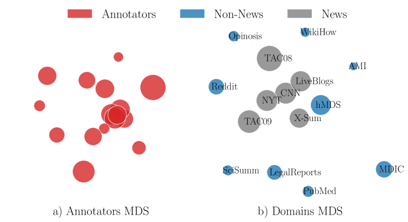
Figure 3: Multi-dimensional scaling projections of (a) annotators and (b) domains. The Euclidean distance in the projected space represents KL divergence in the original space. The disk size is proportional to how well the $K$ performs on the full TAC datasets, as evaluated by the correlation (Kendall’s $\tau$) between the induced $\theta_{K}$ and human judgments.

Instead of analyzing only news datasets with human annotations (like TAC), we can infer background knowledge from any summarization dataset from any domain as long as document–summary pairs are observed. To illustrate this, we consider a large collection of datasets covering domains such as news, legal documents, product reviews, Wikipedia articles, etc. These do not contain human annotations, so we employ our ms$|$d algorithm to infer a $K$ specific to each dataset. The detailed description of these datasets is given in Appendix C.

Structure of differences. To visualize the differences between annotators, we embed them in 2D using MDS with two annotators being close if their $K$ are similar. In Fig. 3 (a), each annotator is a dot whose size is proportional to how well its $K$ generalizes to the rest of the TAC datasets, as evaluated by the correlation (Kendall’s $\tau$) between the induced $\theta_{K}$ and human judgments. The same procedure is applied to domains and is depicted in Fig. 3 (b).

News datasets appear at the center of all domains meaning that the news domain can be seen as an “average” of the peripheral non-news domains. Furthermore, the $K$’s trained on different news datasets are close to each other, indicating a good level of intra-domain transfer; and unsurprisingly, news datasets also exhibit the best transfer performance on TAC.

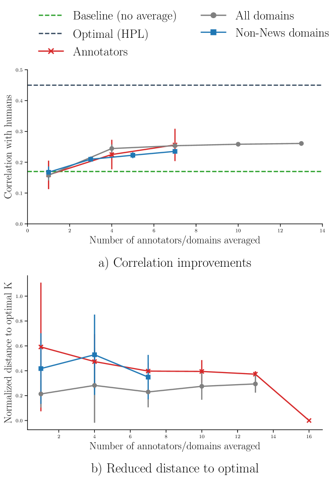
Figure 4: (a) Correlation with human judgments on TAC datasets (news domain) resulting from averaging annotator-specific $K$’s and domain-specific $K$’s. (b) Distance to the optimal $K$ (computed by running hpl on the full TAC datasets).

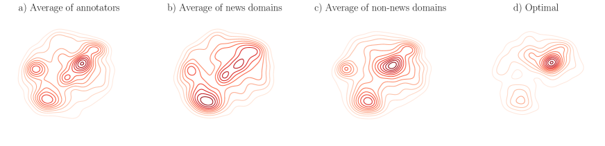
Figure 5: Several $K$ distributions visualized as density in 2D GloVe embedding space.

Improvements due to averaging. Based on previous observations, we make the hypothesis that averaging different annotator-specific $K$’s can lead to better correlation with human judgments on the unseen part of the TAC dataset. Similarly, news domains generalize better than other domains. We hypothesized that averaging domains may also result in improved correlations with humans in the news domain.

In Fig. 4(a), we report the improvements in correlation with human judgments on TAC (news domain) resulting from averaging an increasing number of annotators or domains. The error bars represent $95\%$ confidence intervals arising from selecting a different subset to compute the average. As we see, increasing the number of annotators averaged results in clear and significant improvements. Since the error bars are small, which annotators are included in the averaging has little impact on the results.

Similarly, averaging different domains also results in significant improvements. In particular, averaging several non-news domains gives better generalization to the news domain.

Furthermore, Fig. 5 shows, in the GloVe Pennington et al. (2014) embedding space, the $K$’s resulting from averaging (a) all annotators ($K$’s inferred by hpl), (b) all news datasets ($K$’s inferred by ms$|$d), and (c) all non-news datasets ($K$’s inferred by ms$|$d) in comparison to (d) the optimal $K$ learned with hpl trained on all data from TAC datasets. To produce these visualizations, we perform a density estimation of the $K$’s in the 2D projection of word embeddings.

All averaged $K$’s tend to be similar to the optimal $K$. It indicates that only one prior produces strong results on the news datasets and it can be obtained by averaging many biased but different $K$’s. This is further confirmed by Fig. 4(b), where the distance to the optimal $K$ (measured in terms of KL divergence) significantly decreases when more annotators are averaged.

8 Conclusion

We focus on the often-ignored background knowledge for summarization and infer it from implicit signals from human summarizers and annotators. We introduced and evaluated different approaches, observing strong abilities to fit the data.

The newly-gained ability to infer interpretable priors on importance in a data-driven way has many potential applications. For example, we can describe which topics should be extracted more frequently by systems to improve their agreement with humans. Using pretrained priors also helps systems to reduce overfitting on the frequency signal within source documents as illustrated by initial results in Appendix D.

An important application made possible by this framework is to infer $K$ on any meaningful subset of the data. In particular, we learned annotator-specific $K$’s, which yielded interesting insights: some annotators exhibit large differences from the others, and averaging several, potentially biased $K$’s results in generalization improvements. We also inferred $K$’s from different summarization datasets and also found increased performance on the news domain when averaging $K$’s from diverse domains.

For future work, different choices of semantic units can be explored, e.g., learning $K$ directly in the embedding space. Also, we fixed $\alpha=\beta=1$ to get comparable results across methods, but including them as learnable parameters could provide further performance boosts. Investigating how to infuse the fitted priors into summarization systems is another promising direction.

More generally, inferring $K$ from a common-sense task like summarization can provide insights about general human importance priors. Inferring such priors has applications beyond summarization, as the framework can model any information selection task.

Appendix A 2D Visualization of $K$

For each annotator and each domain, we produce visualizations in the 2D embedding space with the same procedure as in Fig. 5. Fig. 6 depicts the annotators and Fig. 7 depicts the domains. It is interesting to observe much more diversity resulting from the domains and the domain-specific $K$’s are more spread out in the semantic space. This reflects the greater topic diversity discussed in different domains. In contrast, each annotator’s $K$ is inferred based on the TAC datasets, which are in the same domain (news).

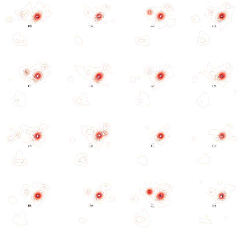
Figure 6: Visualization of each annotator’s $K$ based on 2D projection of Glove word embedding.

Figure 7: Visualization of each domain’s $K$ based on 2D projection of Glove word embedding.

Appendix B Derivation of Approaches

The direct score maximization model consists in maximizing:

$$\mathcal{L}=\sum\limits_{x}\theta_{K}(x)-\gamma\cdot\textsc{{kl}}(P||K),$$ (9)

We use Lagrange multipliers with the constraint that $K$ is a valid distribution:

$$L=$$

$$\sum\limits_{x}\theta_{K}(x)-\gamma\cdot\textsc{{kl}}(P||K)-\lambda\left(\sum\limits_{\omega_{j}}\mathbb{P}_{K}(\omega_{j})-1\right)$$ (10)

(ms$|$u) First, with $P=U$ the uniform and $\gamma\neq 0$, we have the following derivatives:

$$\frac{d\theta_{K}(x_{i})}{d\mathbb{P}_{K}(\omega_{j})}=-\frac{\mathbb{P}_{S_{i}}(\omega_{j})}{\mathbb{P}_{K}(\omega_{j})}$$ (11)

$$\frac{d\gamma\cdot\textsc{{kl}}(U||K)}{d\mathbb{P}_{K}(\omega_{j})}=-\frac{\gamma}{\mathbb{P}_{K}(\omega_{j})}$$ (12)

$$\frac{dL}{d\mathbb{P}_{K}(\omega_{j})}=-\sum\limits_{x}\frac{\mathbb{P}_{S_{i}}(\omega_{j})}{\mathbb{P}_{K}(\omega_{j})}+\frac{\gamma}{\mathbb{P}_{K}(\omega_{j})}-\lambda$$ (13)

Setting the Lagrange derivative to $0$ yields:

$$\mathbb{P}_{K}(\omega_{j})=\frac{1}{\lambda}\left(\gamma-\sum\limits_{x}\mathbb{P}_{S_{i}}(\omega_{j})\right),$$ (14)

where $\lambda$ is the normalizing constant. In particular, when $\gamma=1$:

$$\mathbb{P}_{K}(\omega_{j})=\frac{1}{\lambda}\left(1-\sum\limits_{x}\mathbb{P}_{S_{i}}(\omega_{j})\right).$$ (15)

Note that choosing $\gamma\geq 1$ ensures that for all $\omega_{j}$, we have $\mathbb{P}_{K}(\omega_{j})>0$.

(ms$|$d) Second, we consider the case $P=D$ the document and $\gamma\neq 0$. $U$ changes with every document-summary pair and $\mathcal{L}$ becomes:

$$\mathcal{L}=\sum\limits_{(D,S)}\theta(x)-\sum\limits_{(D,S)}\textsc{{kl}}(D||K),$$ (16)

Then, only the the derivative concerning $\textsc{{kl}}(U||K)$ is modified and becomes:

$$\frac{d\gamma\cdot\textsc{{kl}}(D||K)}{d\mathbb{P}_{K}(\omega_{j})}=-\frac{\gamma\cdot\mathbb{P}_{D}(\omega_{j})}{\mathbb{P}_{K}(\omega_{j})}$$ (17)

which gives the following solution after setting the Lagrange derivative to $0$:

$$\mathbb{P}_{K}(\omega_{j})=\frac{1}{\lambda}\left(\sum\limits_{x}\gamma\cdot\mathbb{P}_{D_{i}}(\omega_{j})-\mathbb{P}_{S_{i}}(\omega_{j})\right).$$ (18)

Here it is not clear that $\mathbb{P}_{K}(\omega_{j})$ is positive for every units. To avoid such issue, notice that we can choose $\gamma\geq\min_{j}\frac{\mathbb{P}_{S}(\omega_{j})}{\mathbb{P}_{D}(\omega_{j})}$.

Appendix C Datasets

The summarization track at the Text Analysis Conference (TAC) was a direct continuation of the DUC series. In particular, the main tasks of TAC-2008 Dang and Owczarzak (2008b) and TAC-2009 Dang and Owczarzak (2009b) were refinements of the pilot update summarization task of DUC 2007. A dataset of 48 topics was released as part of the 2008 edition and 44 new topics were created in 2009. TAC-2008 and TAC-2009 became standard benchmark datasets.

The New York Times Annotated Corpus Sandhaus (2008) counts as one of the largest summarization datasets currently available. It contains nearly 1 million carefully selected articles from the New York Times, each with summaries written by humans.

Also, the CNN/Daily Mail dataset Hermann et al. (2015) has been decisive in the recent development of neural abstractive summarization See et al. (2017); Paulus et al. (2017); Cheng and Lapata (2016). It contains CNN and Daily Mail articles together with bullet point summaries.

Zopf et al. (2016) also viewed the high-quality Wikipedia featured articles as summaries, for which potential sources were automatically searched on the web.

P.V.S. et al. (2018) recently crawled the live-blog archives from the BBC and The Guardian together with some bullet-point summaries reporting the main developments of the event covered.

To evaluate their opinion-oriented summarization system, Ganesan et al. (2010) constructed the Opinosis dataset. It contains 51 articles discussing the features of commercial products (e.g., iPod’s Battery Life).

Furthermore, we consider the large PubMed dataset Cohan et al. (2018), a collection of scientific publications.

The Reddit dataset Kim et al. (2019) has been collected on popular sub-reddits.

The AMI corpus Carletta et al. (2005) is a standard product review summarization dataset.

Koupaee and Wang (2018) automatically crawled the WikiHow website using the self-reported bullet points as summaries.

The XSUM dataset Narayan et al. (2018) is a large collection of news articles with a focus on abstractive summaries.

To measure the effect of information distortion in summarization cascades of scientific results, Horta Ribeiro et al. (2019) collected manual summaries of various lengths.

We also included the LegalReport dataset Galgani et al. (2012) where the task is to summarize legal documents.

Dataset	Creation	Input		Summary	Size
	Man./Auto.	Type	Genre	Length	Topics	Doc/Topic
TAC-2008	M	MDS	News	100	48	10
TAC-2009	M	MDS	News	100	44	10
SciSumm	A	MDS	Sci.	150	1000	1
CNN/Daily Mail	A	SDS	News	$\approx$50	$\approx$300K	1
NYT Corpus	A	SDS	News	$\approx$50	$\approx$650K	1
Opinosis	M	MDS	Review	$\approx$20	51	$\approx$100
LiveBlogs	A	Temporal	Snippets	$\approx$60	$\approx$2K	$\approx$70
hMDS	M	MDS	Heter.	$\approx$216	91	$\approx$14
PUBMED	A	SDS	Sci.	$\approx$100	$\approx$133K	1
XSUM	A	SDS	News	$\approx$25	$\approx$220K	1
Reddit	A	SDS	Heter.	$\approx$20	$\approx$122K	1
AMI	M	MDS	Meeting	$\approx$280	137	10
WikiHow	A	SDS	Heter.	$\approx$60	$\approx$230K	1
LegalReports	A	SDS	Legal	$\approx$280	3500	1
MDIC	M	Cascade	Sci.	varying	16	1

Table 3: Description of datasets used in the experiments

Appendix D Extracting Summaries: Example

Once $K$ is specified, the summary scoring function $\theta_{K}$ can be used to extract summaries. For extractive summarization, this is an optimal subset selection problem McDonald (2007). Unfortunately, $\theta_{K}$ is not linear and cannot be optimized with Integer Linear Programming. It is also not submodular and cannot be optimized with the greedy algorithm for submodularity. We have to rely on generic optimization techniques which do not make any assumption about the objective function and can approximately optimize any arbitrary function. We use the genetic algorithm proposed by Peyrard and Eckle-Kohler (2016) which creates and iteratively optimizes summaries over time. We denote as ($\theta_{K}$, Gen) the summarization system approximately solving the subset selection problem. We compare $3$ systems: when $K$ is inferred by ms|d, when $K$ is inferred by hpl and when $K$ is the uniform distribution. For reference, we report the standard summarization baselines described in the previous section. The summaries are evaluated with 2 automatic evaluation metrics: ROUGE-2 recall with stopwords removed (R-2) Lin (2004) and a recent BERT-based evaluation metric (MOVER) Zhao et al. (2019). The results, reported in Table 4, are encouraging since the systems based on the learned priors outperform the uniform prior. They also perform well in comparison to baselines. The inferred prior can benefit systems by preventing them from overfitting on the frequency signal.

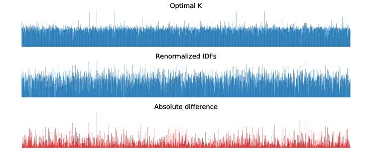
(a) Visualization of optimal $K$, renormalized idf and their absolute difference. One bar for word in the support ($2000$ words).

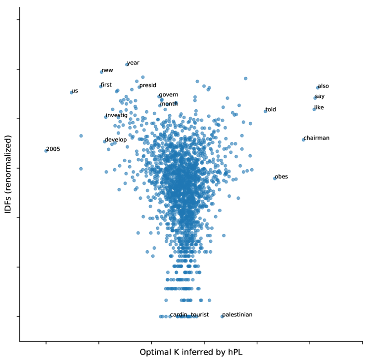
(b) Scatter-plot where each dot is a word and the coordinates are its probability in $K$ and its renomalized idf.

	TAC-08		TAC-09
	R-2	MOVER	R-2	MOVER
Baselines
lr	.078	.336	.090	.360
icsi	.101	.377	.103	.369
kl-greedy	.074	.294	.069	.289
(js, Gen)	.101	.375	.104	.373
Ours
($\theta_{U}$, Gen)	.098	.353	.094	.359
($\theta_{\textsc{{ms|d}}}$, Gen)	.101	.367	.102	.371
($\theta_{\textsc{{hpl}}}$, Gen)	.104	.377	.103	.374

Table 4: Comparison of summarization systems based on maximizing the summary scoring function $\theta_{K}$ induced by different background knowledge.

Appendix E Comparison: IDF vs. optimal $K$

To verify that our inferred $K$ contains different information from id, we compare idf and our optimal $K$ (see Sec. 7).

To be comparable, idf weights need to be renormalized, as the idf weights of known (unknown) words would be low (high) whereas $\mathbb{P}_{K}$ would be high (low). Thus, we compute $\frac{1}{C}(1-\textsc{{idf}}(\omega_{j}))$ for each word $\omega_{j}$, where $C=\sum_{j}(1-\textsc{{idf}}(\omega_{j}))$.

In Fig. 8(a), we represent the full distributions over all words in the support of $K$ and show the absolute difference with renormalized idf weights. Furthermore, Fig. 8(b) is a scatter plot where each dot represent a word and the coordinates are its idf and $K$ weights. The low correlation between the two indicates that $K$ learns a different signal than idf.

References

- Carletta et al. (2005) Jean Carletta, Simone Ashby, Sebastien Bourban, Mike Flynn, Mael Guillemot, Thomas Hain, Jaroslav Kadlec, Vasilis Karaiskos, Wessel Kraaij, Melissa Kronenthal, Guillaume Lathoud, Mike Lincoln, Agnes Lisowska, Iain McCowan, Wilfried Post, Dennis Reidsma, and Pierre Wellner. 2005. The AMI Meeting Corpus: A Pre-Announcement. In Proceedings of the Second International Conference on Machine Learning for Multimodal Interaction, page 28–39, Berlin, Heidelberg. Springer-Verlag.
- Cheng and Lapata (2016) Jianpeng Cheng and Mirella Lapata. 2016. Neural Summarization by Extracting Sentences and Words. In Proceedings of the 54th Annual Meeting of the Association for Computational Linguistics (Volume 1: Long Papers), pages 484–494. Association for Computational Linguistics.
- Cohan et al. (2018) Arman Cohan, Franck Dernoncourt, Doo Soon Kim, Trung Bui, Seokhwan Kim, Walter Chang, and Nazli Goharian. 2018. A Discourse-Aware Attention Model for Abstractive Summarization of Long Documents. In Proceedings of the 2018 Conference of the North American Chapter of the Association for Computational Linguistics: Human Language Technologies, Volume 2 (Short Papers), pages 615–621, New Orleans, Louisiana. Association for Computational Linguistics.
- Conroy et al. (2006) John M. Conroy, Judith D. Schlesinger, and Dianne P. O’Leary. 2006. Topic-Focused Multi-Document Summarization Using an Approximate Oracle Score. In Proceedings of the COLING/ACL 2006 Main Conference Poster Sessions, pages 152–159, Sydney, Australia. Association for Computational Linguistics.
- Dang and Owczarzak (2008a) Hoa Trang Dang and Karolina Owczarzak. 2008a. Overview of the TAC 2008 update summarization task. In Proceedings of the Text Analysis Conference (TAC) 2008 Workshop - Notebook papers and results, pages 10–23.
- Dang and Owczarzak (2008b) Hoa Trang Dang and Karolina Owczarzak. 2008b. Overview of the TAC 2008 Update Summarization Task. In Proceedings of the First Text Analysis Conference (TAC 2008), pages 1–16.
- Dang and Owczarzak (2009a) Hoa Trang Dang and Karolina Owczarzak. 2009a. Overview of the TAC 2009 Summarization Track. In Proceedings of the Text Analysis Conference (TAC), pages 10–23.
- Dang and Owczarzak (2009b) Hoa Trang Dang and Karolina Owczarzak. 2009b. Overview of the TAC 2009 Summarization Track. In Proceedings of the First Text Analysis Conference (TAC 2009), pages 1–12.
- Delort and Alfonseca (2012) Jean-Yves Delort and Enrique Alfonseca. 2012. DualSum: A Topic-model Based Approach for Update Summarization. In Proceedings of the 13th Conference of the European Chapter of the Association for Computational Linguistics, pages 214–223.
- Dunning (1993) Ted Dunning. 1993. Accurate Methods for the Statistics of Surprise and Coincidence. Computational linguistics, 19(1):61–74.
- Erkan and Radev (2004) Günes Erkan and Dragomir R. Radev. 2004. LexRank: Graph-based Lexical Centrality As Salience in Text Summarization. Journal of Artificial Intelligence Research, pages 457–479.
- Galgani et al. (2012) Filippo Galgani, Paul Compton, and Achim Hoffmann. 2012. Citation Based Summarisation of Legal Texts. In PRICAI 2012: Trends in Artificial Intelligence, pages 40–52, Berlin, Heidelberg. Springer Berlin Heidelberg.
- Ganesan et al. (2010) Kavita Ganesan, ChengXiang Zhai, and Jiawei Han. 2010. Opinosis: A Graph Based Approach to Abstractive Summarization of Highly Redundant Opinions. In Proceedings of the 23rd International Conference on Computational Linguistics (Coling 2010), pages 340–348.
- Gao et al. (2018) Yang Gao, Christian M. Meyer, and Iryna Gurevych. 2018. APRIL: Interactively learning to summarise by combining active preference learning and reinforcement learning. In Proceedings of the 2018 Conference on Empirical Methods in Natural Language Processing, pages 4120–4130, Brussels, Belgium. Association for Computational Linguistics.
- Gillick and Favre (2009) Dan Gillick and Benoit Favre. 2009. A Scalable Global Model for Summarization. In Proceedings of the Workshop on Integer Linear Programming for Natural Language Processing, pages 10–18, Boulder, Colorado. Association for Computational Linguistics.
- Haghighi and Vanderwende (2009) Aria Haghighi and Lucy Vanderwende. 2009. Exploring Content Models for Multi-document Summarization. In Proceedings of Human Language Technologies: The 2009 Annual Conference of the North American Chapter of the Association for Computational Linguistics, pages 362–370.
- Harabagiu and Lacatusu (2005) Sanda Harabagiu and Finley Lacatusu. 2005. Topic Themes for Multi-document Summarization. In Proceedings of the 28th Annual International ACM SIGIR Conference on Research and Development in Information Retrieval, pages 202–209.
- Hermann et al. (2015) Karl Moritz Hermann, Tomas Kocisky, Edward Grefenstette, Lasse Espeholt, Will Kay, Mustafa Suleyman, and Phil Blunsom. 2015. Teaching Machines to Read and Comprehend. In Advances in Neural Information Processing Systems 28, pages 1693–1701.
- Hong and Nenkova (2014) Kai Hong and Ani Nenkova. 2014. Improving the Estimation of Word Importance for News Multi-Document Summarization. In Proceedings of the 14th Conference of the European Chapter of the Association for Computational Linguistics, pages 712–721, Gothenburg, Sweden. Association for Computational Linguistics.
- Horta Ribeiro et al. (2019) Manoel Horta Ribeiro, Kristina Gligoric, and Robert West. 2019. Message Distortion in Information Cascades. In The World Wide Web Conference, page 681–692, New York, NY, USA. Association for Computing Machinery.
- Kim et al. (2019) Byeongchang Kim, Hyunwoo Kim, and Gunhee Kim. 2019. Abstractive Summarization of Reddit Posts with Multi-level Memory Networks. In Proceedings of the 2019 Conference of the North American Chapter of the Association for Computational Linguistics: Human Language Technologies, Volume 1 (Long and Short Papers), pages 2519–2531, Minneapolis, Minnesota. Association for Computational Linguistics.
- Koupaee and Wang (2018) Mahnaz Koupaee and William Yang Wang. 2018. WikiHow: A Large Scale Text Summarization Dataset. CoRR abs/1810.09305.
- Lin (2004) Chin-Yew Lin. 2004. ROUGE: A Package for Automatic Evaluation of Summaries. In Text Summarization Branches Out: Proceedings of the ACL-04 Workshop, pages 74–81, Barcelona, Spain. Association for Computational Linguistics.
- Liu and Singh (2004) Hugo Liu and Push Singh. 2004. ConceptNet — A Practical Commonsense Reasoning Tool-Kit. BT Technology Journal, 22(4):211–226.
- Louis (2014) Annie Louis. 2014. A Bayesian Method to Incorporate Background Knowledge during Automatic Text Summarization. In Proceedings of the 52nd Annual Meeting of the Association for Computational Linguistics (Volume 2: Short Papers), pages 333–338, Baltimore, Maryland.
- Luhn (1958) Hans Peter Luhn. 1958. The Automatic Creation of Literature Abstracts. IBM Journal of Research Development, 2:159–165.
- Mani (1999) Inderjeet Mani. 1999. Advances in Automatic Text Summarization. MIT Press, Cambridge, MA, USA.
- Maystre (2018) Lucas Maystre. 2018. Efficient Learning from Comparisons. EPFL, Lausanne.
- McDonald (2007) Ryan McDonald. 2007. A Study of Global Inference Algorithms in Multi-document Summarization. In Proceedings of the 29th European Conference on Information Retrieval Research, pages 557–564.
- Narayan et al. (2018) Shashi Narayan, Shay B. Cohen, and Mirella Lapata. 2018. Don’t Give Me the Details, Just the Summary! Topic-Aware Convolutional Neural Networks for Extreme Summarization. In Proceedings of the 2018 Conference on Empirical Methods in Natural Language Processing, pages 1797–1807, Brussels, Belgium. Association for Computational Linguistics.
- Nenkova and Passonneau (2004) Ani Nenkova and Rebecca Passonneau. 2004. Evaluating Content Selection in Summarization: The Pyramid Method. In Proceedings of the Human Language Technology Conference of the North American Chapter of the Association for Computational Linguistics (HLT-NAACL), pages 145–152, Boston, Massachusetts, USA.
- Paulus et al. (2017) Romain Paulus, Caiming Xiong, and Richard Socher. 2017. A Deep Reinforced Model for Abstractive Summarization. CoRR abs/1705.04304.
- Pennington et al. (2014) Jeffrey Pennington, Richard Socher, and Christopher Manning. 2014. Glove: Global Vectors for Word Representation. In Proceedings of the 2014 Conference on Empirical Methods in Natural Language Processing (EMNLP), pages 1532–1543, Doha, Qatar. Association for Computational Linguistics.
- Peyrard (2019) Maxime Peyrard. 2019. A Simple Theoretical Model of Importance for Summarization. In Proceedings of the 57th Annual Meeting of the Association for Computational Linguistics, pages 1059–1073, Florence, Italy. Association for Computational Linguistics.
- Peyrard and Eckle-Kohler (2016) Maxime Peyrard and Judith Eckle-Kohler. 2016. A General Optimization Framework for Multi-Document Summarization Using Genetic Algorithms and Swarm Intelligence. In Proceedings of the 26th International Conference on Computational Linguistics (COLING), pages 247 – 257.
- P.V.S. et al. (2018) Avinesh P.V.S., Maxime Peyrard, and Christian M. Meyer. 2018. Live Blog Corpus for Summarization. In Proceedings of the 11th International Conference on Language Resources and Evaluation, pages 3197–3203.
- Riedhammer et al. (2010) Korbinian Riedhammer, Benoit Favre, and Dilek Hakkani-Tür. 2010. Long Story Short - Global Unsupervised Models for Keyphrase Based Meeting Summarization. Speech Communication, 52(10):801–815.
- Sandhaus (2008) Evan Sandhaus. 2008. The New York Times Annotated Corpus. Linguistic Data Consortium, Philadelphia, 6(12).
- See et al. (2017) Abigail See, Peter J. Liu, and Christopher D. Manning. 2017. Get To The Point: Summarization with Pointer-Generator Networks. In Proceedings of the 55th Annual Meeting of the Association for Computational Linguistics (Volume 1: Long Papers), pages 1073–1083, Vancouver, Canada. Association for Computational Linguistics.
- Sparck Jones (1972) Karen Sparck Jones. 1972. A Statistical Interpretation of Term Specificity and its Application in Retrieval. Journal of documentation, 28(1):11–21.
- Zhao et al. (2019) Wei Zhao, Maxime Peyrard, Fei Liu, Yang Gao, Christian M. Meyer, and Steffen Eger. 2019. MoverScore: Text generation evaluating with contextualized embeddings and earth mover distance. In Proceedings of the 2019 Conference on Empirical Methods in Natural Language Processing and the 9th International Joint Conference on Natural Language Processing (EMNLP-IJCNLP), pages 563–578, Hong Kong, China. Association for Computational Linguistics.
- Zopf et al. (2016) Markus Zopf, Maxime Peyrard, and Judith Eckle-Kohler. 2016. The Next Step for Multi-Document Summarization: A Heterogeneous Multi-Genre Corpus Built with a Novel Construction Approach. In Proceedings of the 26th International Conference on Computational Linguistics: Technical Papers, pages 1535–1545.