Towards a self-consistent analysis of the anisotropic galaxy two- and three-point correlation functions on large scales: application to mock galaxy catalogues
Abstract
We establish a practical method for the joint analysis of anisotropic galaxy two- and three-point correlation functions (2PCF and 3PCF) on the basis of the decomposition formalism of the 3PCF using tri-polar spherical harmonics. We perform such an analysis with MultiDark Patchy mock catalogues to demonstrate and understand the benefit of the anisotropic 3PCF. We focus on scales above , and use information from the shape and the baryon acoustic oscillation (BAO) signals of the 2PCF and 3PCF. We also apply density field reconstruction to increase the signal-noise ratio of BAO in the 2PCF measurement, but not in the 3PCF measurement. In particular, we study in detail the constraints on the angular diameter distance and the Hubble parameter. We build a model of the bispectrum or 3PCF that includes the nonlinear damping of the BAO signal in redshift space. We carefully account for various uncertainties in our analysis including theoretical models of the 3PCF, window function corrections, biases in estimated parameters from the fiducial values, the number of mock realizations to estimate the covariance matrix, and bin size. The joint analysis of the 2PCF and 3PCF monopole and quadrupole components shows a and improvement in Hubble parameter constraints before and after reconstruction of the 2PCF measurements, respectively, compared to the 2PCF analysis alone. This study clearly shows that the anisotropic 3PCF increases cosmological information from galaxy surveys and encourages further development of the modeling of the 3PCF on smaller scales than we consider.
keywords:
cosmology: large-scale structure of Universe – cosmology: dark matter – cosmology: observations – cosmology: theory1 INTRODUCTION
Baryon Acoustic Oscillations (BAOs) are a powerful tool for measuring the expansion history of the Universe. In particular, the anisotropic signal of BAO via the Alcock-Paczyński (AP) effect (Alcock & Paczyński, 1979) provides an extremely important means of measuring the angular diameter distance and the expansion rate at each redshift separately. As dark energy, one of the most mysterious aspects of cosmology, mainly affects the cosmic expansion history of the universe, robust estimates of and via the anisotropic BAO will lead to an accurate probe of dark energy.
Eisenstein et al. (2005) reported the first unambiguous detection of the baryon acoustic peak in the galaxy two-point correlation function (2PCF) using spectroscopic samples of luminous red galaxies from the Sloan Digital Sky Survey (SDSS) (Eisenstein et al., 2001). Since this first detection, much effort has been put into measuring the BAO signature for the samples of galaxies (Tegmark et al., 2006; Okumura et al., 2008; Percival et al., 2010; Blake et al., 2011a; Beutler et al., 2011; Blake et al., 2011b; Seo et al., 2012; Padmanabhan et al., 2012; Anderson et al., 2013; Xu et al., 2013; Anderson et al., 2014; Tojeiro et al., 2014; Ross et al., 2015; Beutler et al., 2017a; Zhao et al., 2017), galaxy clusters (Veropalumbo et al., 2016) and quasars (du Mas des Bourboux et al., 2017; Zhu et al., 2018). More recently, the accuracy of the BAO data has been further improved by precise measurements in the Baryon Oscillation Spectroscopic Survey (BOSS; Eisenstein et al. 2011; Bolton et al. 2012; Dawson et al. 2013) Data Release 12 (DR12; Alam et al. 2015). Currently, the precision on and obtained from the 2PCF and its Fourier counter part, the power spectrum, is on the order of - percent and - percent before reconstruction, and - percent and - percent after reconstruction (e.g., Alam et al. 2017). Future missions such as the Subaru Prime Focus Spectrograph (PFS; Takada et al. 2014), the Dark Energy Spectroscopic Instrument (DESI; Levi et al. 2013) and the space-based Euclid mission (Laureijs et al., 2011) are expected to provide unprecedentedly accurate measurements of and .
Based on the great success of the analysis of the two-point statistics, there is a growing interest in using measurements of the three-point function (3PCF) or its Fourier counter part, the bispectrum for the cosmological data analysis (as recent works, see e.g. Hahn et al., 2020; Gualdi & Verde, 2020). There have been several studies on cosmological analysis using the three-point statistics, but they dealt only with the isotropic component of the three-point statistics, i.e., the monopole component. For example, Slepian et al. (2017) successfully detected a -level BAO signal from BOSS DR12 data using the 3PCF, and Pearson & Samushia (2018) also detected a -level BAO signal from the same data using the bispectrum. In the combined analysis of the two- and three-point statistics, Pearson & Samushia (2018) reported an improvement of for the volume-averaged angular diameter distance ; Gil-Marĺn et al. (2017) reported the results of a joint analysis using the monopole and quadrupole power spectra and the monopole bispectrum.
Now, it is time to analyze the anisotropic component of the 3PCF or bispectrum, i.e., the quadrupole component. In order to do so, we have several problems to solve. The first problem is how to characterize and decompose the anisotropic components. For example, adopting the plane-parallel approximation, the redshift-space 3PCF depends on two relative coordinate vectors and one line-of-sight (LOS) unit vector. With three angular dependences, the choice of coordinate system to characterize the anisotropy of the 3PCF is arbitrary. Although decomposition methods dependent on a specific coordinate system have been proposed by Scoccimarro et al. (1999); Slepian & Eisenstein (2018), in this paper, we will adopt a coordinate system-independent formalism using the tri-polar spherical harmonics (TripoSH) proposed by Sugiyama et al. (2019). The second issue is the impact of survey geometry on the 3PCF and bispectrum. Since we measure the 3PCF and bispectrum using an estimator based on the Fast Fourier Transform (FFT) proposed by Scoccimarro (2015); Slepian & Eisenstein (2016); Sugiyama et al. (2019), the measured 3PCF and bispectrum contain the effects of survey geometry. In particular, survey geometry can distort the observed density fluctuations and introduce spurious anisotropic signals. Therefore, we need to compute a theoretical model of the 3PCF or bispectrum corrected for the effects of survey geometry, following the method proposed by Sugiyama et al. (2019). Third, we need to construct a theoretical model to predict the galaxy 3PCF or bispectrum in redshift space. There are several empirical models of the monopole bispectrum (3PCF) applied to the actual BOSS dataset (Slepian & Eisenstein, 2017; Gil-Marín et al., 2015; Pearson & Samushia, 2018), which take into account the non-linear damping of BAO by replacing linear power spectra appearing in a tree-level based solution with non-linear power spectra. Since the non-linear effect on BAO is well understood in the power spectrum (2PCF) using cosmological perturbation theory (e.g., Crocce & Scoccimarro, 2008; Matsubara, 2008a), it is desirable to have a model that can explain the BAO damping based on the perturbation theory for the bispectrum (3PCF) as well. Furthermore, it is intrinsically important to be able to quickly compute the theoretical model, as cosmological analysis using e.g. Markov-Chain Monte Carlo (MCMC) algorithm requires tens or hundreds of thousands of iterations of theoretical models with different cosmological parameters. The forth is the relationship between the number of binned measurement data, the number of realizations of the mock simulation that reproduce the observed data, and the number of fitting parameters. To estimate the covariance matrix of the observed data, brute-force methods using a huge number of mock simulations are commonly used. The number of simulations required to compute a reliable covariance matrix depends on the number of data and fitting parameters (Hartlap et al., 2007; Percival et al., 2014). To perform a conservative analysis, one must either reduce the number of data and fitting parameters for a given number of simulations or increase the number of simulations for a given number of data and fitting parameters. Alternatively, one idea is to use an analytic model of the covariance matrix that corresponds to the results obtained from an infinite number of realizations, which is being vigorously studied (Sugiyama et al., 2020; Philcox & Eisenstein, 2019).
The aim of this paper is to establish a self-consistent cosmological analysis method using the anisotropic component of the 3PCF by solving all the four problems, for the first time. As the first and second problems have been already addressed by Sugiyama et al. (2019), we focus on the third and forth ones in this paper. We propose a simple template model of the galaxy bispectrum in redshift space as an analogy of the power spectrum template model presented by Eisenstein et al. (2007a). That is, our bispectrum template model restores a tree-level solution consisting of a smooth version (without BAO) of the linear power spectrum after degrading the BAO signature. We then develop an approximation method to compute the bispectrum template model fast, taking into account the window function correction. The specific form of the bispectrum model is as follows:
| (1) |
where , and denote wavevectors, and represents the LOS unit vector. The first order kernel function in the standard perturbation theory (for a review, see Bernardeau et al., 2002) is the so-called Kaiser formula of linear redshift space distortions (RSD; Kaiser, 1987; Hamilton, 1997), where and are the linear bias parameter and the logarithmic growth rate function , respectively. The second order kernel function depends on the non-linear gravity effect, non-linear redshift-space distortion effect, and the non-linear bias effect. For the BAO signal in the linear matter power spectrum , the “no-wiggle (nw)” part is a smooth version of with the baryon oscillations removed (Eisenstein & Hu, 1998), and the “wiggle (w)” part is defined as . The non-linear BAO degradation is represented by the two-dimensional Gaussian damping factor derived from an differential motions of Lagrangian displacements (Eisenstein & Hu, 1998; Crocce & Scoccimarro, 2006; Matsubara, 2008a): , where , and and are the radial and transverse components of smoothing parameters.
We perform data analysis on the MultiDark-Patchy mock catalogues (MD-Patchy mocks; Klypin et al., 2016; Kitaura et al., 2016) using the 2PCF and 3PCF. The reason of this choice is because the MultiDark-Patchy mock catalogues and the cosmological constraints on 2PCF or the power spectrum are well studied in previous works (Ross et al., 2017; Satpathy et al., 2017). We limit the scale of interest to and above. This restriction allows us to capture all the BAO signals appearing around , while still maintaining the validity of the template model of the 2PCF and 3PCF based on tree-level solutions (linear theory for the 2PCF and the second-order perturbation theory for the 3PCF) thanks to small non-linearities. Note that our analysis in principle can serve as a RSD analysis, since the theoretical model we use does not include any unphysical nuisance parameters, and we can also constrain the growth rate parameter. However, since we use only large scales, our RSD constraints are not expected to be competitive with previous studies (Satpathy et al., 2017; Beutler et al., 2017b), and hence are not main focus of this paper.
The methods for reducing the number of data bins are as follows. First, we use the 2PCF and 3PCF only around the BAO scale (). For example, in the case of the power spectrum, the BAO signal appears as an oscillation function up to . Therefore, in order to analyze BAO in the power spectrum, it is common to fit the broadband shape up to small scales, using some nuisance parameters. A similar analysis can be performed in the bispectrum, but the number of data bins required increases dramatically because the bispectrum depends on two scales. Thus, the 3PCF is more useful than the bispectrum in terms of reducing the number of data bins. Second, we adopt a wider bin size for the 3PCF than for the 2PCF in order for the compression of data. Specifically, we use a bin width of for the 2PCF, which is considered by e.g. Ross et al. (2017) to be a fiducial bin size, but for the 3PCF, we adopt a wider bin width of . Finally, when analyzing the data, we find a minimal combination of data by examining which coefficients in the TripoSH decomposition of the 3PCF have the main information on the anisotropic BAO. Through these efforts, we manage to keep the parameter (105), which corrects for the effect on the variance of the estimated parameters due to the fact that the number of the MD-Patchy mocks is finite (), to .
We apply the density field reconstruction to the 2PCF measurements. The reconstruction was originally proposed to enhance the BAO signal in 2PCF (Eisenstein et al., 2007b), but it is also known to reduce the non-Gaussian terms of the covariance matrix due to its ability to partially remove nonlinear gravity (Beutler et al., 2017b). Thus, it is expected to reduce the statistical error of the entire parameter of interest, in addition to the BAO signal. The reconstruction employed in this paper is the simplest one and does not remove the linear RSD effect. As a result, at the large scales above that we focus on, the shape of the 2PCF can be evaluated by linear theory, except for the BAO smoothing parameter. In other words, we can use Eisenstein et al. (2007a)’ template power spectrum model for theoretical predictions of the 2PCF even after reconstruction (e.g., White, 2015). Note that our analysis is the first RSD analysis of the post-reconstruction 2PCF and results in a rigorous (again, not competitive, though) constraint on . We do not apply reconstruction to the measurement of the 3PCF because the method for analyzing 3PCFs after reconstruction has not yet been established.
This paper is organized as follows: Section 2 briefly reviews the TripoSH decomposition formalism of the 3PCF and bispectrum; Section 3 builds a bispectrum template model for use in data analysis; Section 4 describes how to correct for the effect of survey geometry when calculating the 3PCF, and an approximation method to compute the 3PCF quickly; Section 5 performs parameter estimation using the 2PCFs before and after reconstruction; Section 6 performs the joint analysis with the 3PCF while checking for various systematic errors; Section 7 summarizes the discussion and conclusions of this paper. Throughout this paper, we adopt a flat CDM cosmology that is the same as used in the Patchy mocks: .
2 Decomposition formalism
We begin with a review of the decomposition formalism of the redshift-space bispectrum introduced by Sugiyama et al. (2019). In general, a function depending on an orientational unit vector can be expanded in the basis of spherical harmonic functions . The power spectrum and bispectrum in redshift space are characterized by and , where k and are wave vectors and the unit vector in the line-of-sight (LOS) direction, respectively. Since and thus depend on the two and three unit vectors, we can expand them using poly-polar spherical harmonics (Varshalovich et al., 1988), i.e., bipolar spherical harmonics (BipoSH; e.g., Hajian & Souradeep, 2003; Shiraishi et al., 2017; Sugiyama et al., 2018; Chiang & Slosar, 2018) for the power spectrum and tri-polar spherical harmonics (TripoSH; e.g., Verde et al., 2000; Bertacca et al., 2018; Sugiyama et al., 2019) for the bispectrum. In particular, under the assumption of the statistical isotropy and parity symmetry of the universe, the -modes appearing in the BipoSH and TripoSH expansions disappear. As a result, we can expand the redshift-space power spectrum using the Legendre polynomial function as follows (e.g., Hamilton, 1997):
| (2) |
For the bispectrum, we define the base function as
| (3) | |||||
with
| (4) |
where the circle bracket with multipole indices, , denotes the Wigner-3j symbol, and expand the redshift-space bispectrum as (Sugiyama et al., 2019)
| (5) |
We note here that the parity symmetry condition restricts to even numbers. The corresponding coefficients are given by
| (6) | |||||
In the multipole expansion method described above, the multipole index characterizes the anisotropy of the power and bispectra along the LOS direction induced by the RSD or AP effect. In the Newtonian limit, this anisotropy is axially symmetric around the LOS direction, and the allowed is restricted to even numbers. In the case of the power spectrum, the first three multipole components, i.e., the monopole (), quadrupole (), and hexadecapole () components, are known to contain almost all the cosmological information (Taruya et al., 2011). The relativistic effect leads to an odd (e.g., Clarkson et al., 2019; Maartens et al., 2020; de Weerd et al., 2020), which we will ignore throughout this paper.
In the case of the bispectrum, when is non-zero, is non-zero. For example, acceptable combinations of () are , , , etc. for , , , , etc. for , , , , etc. for , and , , , etc. for . Note that we define the base function to be a Legendre polynomial function when , i.e., with being the Kronecker delta. Thus, we can regard the bispectrum decomposition formalism considered here as a natural extension of the Legendre expansion of the monopole bispectrum (Szapudi, 2004; Pan & Szapudi, 2005; Slepian & Eisenstein, 2015, 2016). Since this decomposition formalism does not depend on the choice of coordinate system, we can choose any coordinate system that is convenient for numerical calculations, such as a coordinate system with or as the -axis (Scoccimarro et al., 1999; Slepian & Eisenstein, 2018). In addition, this coordinate independence facilitates comparison with the observed bispectrum because it does not matter if the coordinate system used for the measurement is different from that used for the theoretical prediction. In this paper, we choose the following coordinate systems for our theoretical predictions: for the power spectrum,
| (7) |
and for the bispectrum,
| (8) |
where . Then, the multiple integrals in Eq. (6) are single and triple integrals for the power spectrum and bispectrum, respectively. Measuring the power spectrum and bispectrum from the observed data, we use the Cartesian coordinate and choose the north pole as our -axis.
We can expand the two- and three-point correlation functions (2PCF and 3PCF) in the same way as those used for the power and bispectra. The multipole components of the 2PCF and 3PCF are related to the multipole components of the power and bispectra via the Hankel transform as follows:
| (9) |
and
| (10) | |||||
where is the spherical Bessel function at the -th order. These relations mean that and have the same information as and , respectively, facilitating the comparison of the results of the configuration-space and the Fourier-space analyses.
3 Model
In this section, we present a model of the galaxy bispectrum in redshift space that describes by construction the nonlinear damping of BAO in the framework of the Lagrangian perturbation theory. It is known that the nonlinear damping of the BAO signal in density fields such as dark matter particles, halos, and galaxies can be well explained by large-scale coherent flows of objects (e.g., Eisenstein et al., 2007a). In order to mathematically describe such large-scale flows, we need to consider flows with wavelength modes much larger than the scale of interest, i.e., infrared (IR) modes. For this purpose, the Lagrangian view is useful, because the long-wavelength mode of the displacement vector, which is a variable in the Lagrangian picture, corresponds to the IR flow of direct interest (e.g., Matsubara, 2008a). The IR mode can be manipulated to add up to the infinite order of perturbation theory. Namely, it can be treated as non-perturbative, called IR re-summation. On the other hand, in the Eulerian approach, this IR re-summation can be treated by focusing on perturbation solutions of the density field in the high- limit (e.g., Crocce & Scoccimarro, 2008). This is because the high- limit means that the nonlinear modes affecting the scale of interest are much larger than . We build our bispectrum model based on this idea of IR re-summation (e.g., Blas et al., 2016).
To simplify our notation, we omit the angular dependence of the LOS direction due to RSD effects in density fields, statistics, and etc., unless we specify otherwise. We calculate all the linear power spectra used in this paper using CLASS (Blas et al., 2011).
3.1 Lagrangian perturbation theory
In the Lagrangian picture, the displacement field maps the galaxies from the initial Lagrangian coordinate q to the final Eulerian coordinate x via the relation
| (11) |
The observed positions of the galaxies are displaced from their real-space coordinates along the direction of the LOS due to the RSD effect. In this paper, we use the distant observer approximation for the theoretical calculation of the power and bispectra and represent the direction of the LOS as a global direction . The displacement vector including the RSD effect is then given by (e.g., Taylor & Hamilton, 1996)
| (12) |
where the subscript “real” indicates a real space quantity, is the time-derivative of the real-space displacement vector, and is the Hubble parameter. Expanding the displacement field in perturbation theory, the displacement field for each perturbation order in redshift space is given by (Matsubara, 2008a)
| (13) |
where the superscript indicates the quantity of the -th order in perturbation theory, and the linear logarithmic growth rate function is denoted as with being the growth factor of the linear density perturbation. Note that the left-hand sides of Eqs. (12) and (13) omit the angle dependence of the dispacement vector, as mentioned at the beginning of this section.
The galaxy density perturbation is expressed in the Lagrangian picture as (Matsubara, 2008b)
| (14) |
In Fourier space, this is transformed into
| (15) |
where the tilde mark over any quantity denotes the Fourier transform of that quantity. The density perturbation represents the initial distribution of biased objects, such as galaxies, that form later.
We consider the initial density perturbation of biased objects up to second order (for a review, see Desjacques et al., 2018):
| (16) |
with
| (17) |
where and run over the three spatial coordinate labels denoted as , , and , and represents the Kronecker delta. Throughout this paper, we ignore all relevant stochastic terms and assume that can be expanded in terms of the Gaussian linear density perturbation . The Lagrangian bias parameters, , , and , are related to the Eulerian bias parameters, , , and as follows (Baldauf et al., 2012; Saito et al., 2014):
| (18) |
We vary all , and in our data analysis in Section 6. Note that, for a simple presentation purpose, we set , and in Figures 2 and 3.
3.2 Infra-red flows
Consider decomposing the displacement vector into components at the origin and other components:
| (19) |
We refer to this constant vector as the infra-red (IR) flow of galaxies, which is defined as 111There would be nothing wrong with focusing on a certain point other than the origin. However, since we finally compute the quantity taken as an ensemble average, we can consider the origin without loss of generality thanks to statistical translation symmetry.
| (20) |
The density perturbation (14) is then described by
| (21) |
where we assume that the origin does not contribute to the volume integral in Eq. (14). In Fourier space it becomes
| (22) |
Note that assuming the linear IR flow , we can derive the same expression as Eq. (22) in the Eulerian picture by taking the high- limit (Sugiyama & Futamase, 2013; Sugiyama & Spergel, 2014). Thus, focusing on the IR flow is equivalent to considering the high- limit solution in the Eulerian perturbation theory (PT).
If the IR flow is uncorrelated with the density perturbation, it does not affect the -point statistics because of the statistical homogeneity of the universe. For example, the two- and three-point functions, and , are
| (23) | |||||
where means the ensemble average. In Fourier space, the power spectrum and the bispectrum are
| (24) | |||||
This cancellation of the IR flow is known as the high- limit cancellation in the Eulerian PT and has been shown for the power spectrum at the -loop order (Vishniac, 1983; Suto & Sasaki, 1991; Makino et al., 1992), the -loop order (Sugiyama & Spergel, 2014; Sugiyama, 2014; Blas et al., 2013), and any order (Jain & Bertschinger, 1996). This IR flow cancellation is also closely related to the Galilean invariance of the large-scale structure (Scoccimarro & Frieman, 1996; Peloso & Pietroni, 2013; Kehagias & Riotto, 2013; Peloso & Pietroni, 2017).
In general, the IR flow is correlated with the density perturbation, so the cancellation of the IR flow in the -point statistics does not occur completely. Therefore, the nonlinear effects arising from tend to cancel each other out, but their residual terms are likely to have a physical impact on the -point statistics. In Section 3.5, we show how the breaking of the cancellation of the IR effect gives nonlinear corrections to the BAO signal on the redshift-space bispectrum.
3.3 -expansion
A useful method for extracting most of the information about BAO from the -point statistics is to apply the -expansion method (Bernardeau et al., 2008, 2012), also known as the multi-point propagator or the Wiener-Hermite expansion (Matsubara, 1995; Sugiyama & Futamase, 2012), to density fluctuations. The -expansion is an expansion method based on the statistical properties of the observed fluctuations such as density perturbations and velocity fields. The first-order term of the -expansion is defined as a Gaussian distribution, and its higher-order terms describe the departure from the Gaussian distribution. Using the -expansion, we can decompose the -point statistics into parts with and without the mode-coupling integral. The part without the mode-coupling integral has more information about BAO because the linear power spectrum appears directly, while the mode-coupling integral erases the information about BAO. For example, in the case of the power spectrum, the BAO information on the mode-coupling term is only a few per cent or less (e.g., Seo et al., 2008), and such a small effect is negligible in current galaxy surveys such as BOSS. This fact is likely to be true in the case of the bispectrum as well. Therefore, we do not take into account the BAO information in the mode-coupling integral in this paper when we construct the template model for describing the redshift-space bispectrum in Section 3.5.
In the standard PT, the density perturbation is expanded as
| (25) | |||||
where , is the so-called Kaiser factor (Kaiser, 1987), and are the non-linear kernel functions including the non-linear gravity effect, the non-linear RSD effect, and the non-linear bias effect.
Assuming that the linear density perturbation has a Gaussian distribution, i.e., no primordial non-Gaussianity, we define the first-order of the basis function of the -expansion as . Then, the higher-order basis functions are given by
| (26) |
where the superscript means the -th order of the -expansion. Using these basis functions, the density perturbation is expanded as
| (27) | |||||
The corresponding coefficients are expressed using the standard PT kernel functions as (Sugiyama & Futamase, 2012, 2013)
| (28) | |||||
The power spectrum is decomposed into two parts (Crocce & Scoccimarro, 2006, 2008):
| (29) |
where , known as the “two-point propagator”, represents how the information in the initial linear power spectrum propagates to the final non-linear power spectrum, and , called the “mode-coupling term”, represents the coupling between different modes. These two terms are expressed using as (Bernardeau et al., 2008)
| (30) | |||||
The expression of the bispectrum using the -expansion is given by Bernardeau et al. (2008); we classify that in terms of mode-coupling integrals into the following five parts:
| (31) | |||||
where
| (32) |
| (33) | |||||
| (34) | |||||
| (35) | |||||
and
| (36) | |||||
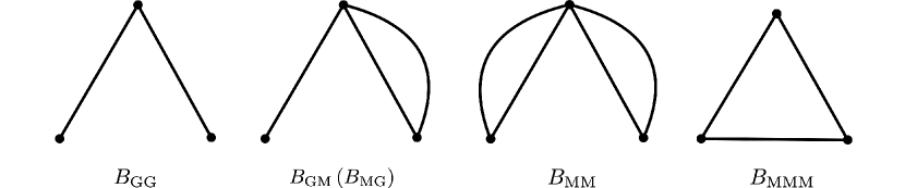
For intuitive understanding, each of the five terms in Eq. (31) is schematically illustrated in Figure 1. The straight line in the figure represents the term proportional to one linear power spectrum, and the closed line represents the mode-coupling effect. The term is proportional to the product of two linear power spectra, the and terms are proportional to the linear power spectrum, and the and terms are composed only of the mode-coupling effect.
3.4 IR cancellation
In this subsection, we demonstrate the IR cancellation by calculating the full order of the -expansion for both the power and bispectra. To see this, consider the linear galaxy perturbation with the linear IR flow
| (37) |
The linear IR flow is described by
| (38) |
where
| (39) |
Eq. (37) means that all nonlinear corrections of the density perturbation at the scale we are interested in are due to long-wavelength (infra-red, IR) modes beyond the scale . To explain Equation (37) in the standard PT context, we assume in Eq. (25) that the amplitude of one of the wave vectors is larger than that of the other, i.e., , resulting in . Then, we obtain
| (40) | |||||
Comparing Eq. (37) and Eq. (40) leads to
| (41) |
Substituting the above equation into Eq. (28) leads to
| (42) |
Here, the damping factor arising from the linear IR flow is given by (Matsubara, 2008a)
| (43) | |||||
where is the dispersion of the linear displacement vector, given by
| (44) |
The propagator term is then expressed as
| (45) |
To compute the mode-coupling term, we assume in the limit in Eq. (30), resulting in
| (46) | |||||
Inserting Eq. (42) in the above expression, we finally derive
| (47) |
and therefore,
| (48) | |||||
This result is as predicted in Eq. (24). The effect of the IR flow on the power spectrum completely is canceled out by summing up all orders of the -expansion, i.e., up to all orders in standard perturbation theory. In other words, in the high- limit, the nonlinear power spectrum becomes just the linear power spectrum.
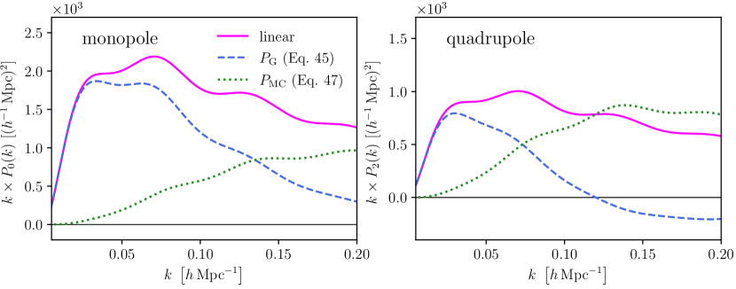
Figure 2 plots the theoretical predictions for the monopole and quadrupole components of the power spectrum in the high- limit, where the sum of the propagator term and the mode-coupling term is the linear theory prediction, as shown in Eq. (48). The propagator of the quadrupole component is negative on small scales. The scale at which the mode-coupling term dominates, i.e., the point at which the theoretical curves of the propagator term and the mode-coupling term intersect, is for the monopole component and for the quadrupole component. This fact shows the intrinsic difficulty of theoretical prediction of the quadrupole component. That is, when focusing on a certain scale , the quadrupole component requires to compute higher-order -expansion terms than the monopole component.
We next turn to the IR cancellation in the bispectrum. As in the case of the power spectrum, consider the second-order density perturbation with the linear IR flow:
| (49) |
The corresponding is given by
| (50) | |||||
where we used the relation
| (51) |
under the condition that the amplitudes of two of momenta, and , are much larger than those of the others: for . Using Eqs. (42) and (50), we derive
| (52) |
| (53) |
| (54) |
| (55) |
| (56) |
where means the tree-level solution of the bispectrum, given by
| (57) |
Obviously, summing up all the five terms , , , and , the nonlinear corrections coming from the IR flow are completely canceled out, and the resulting bispectrum is the same as the tree-level solution.
| (58) |
This ends the proof.
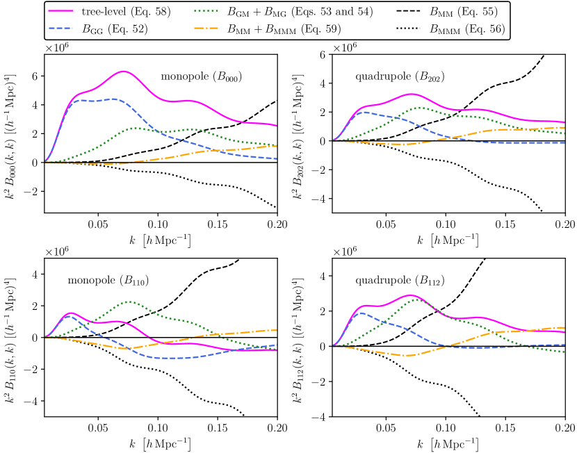
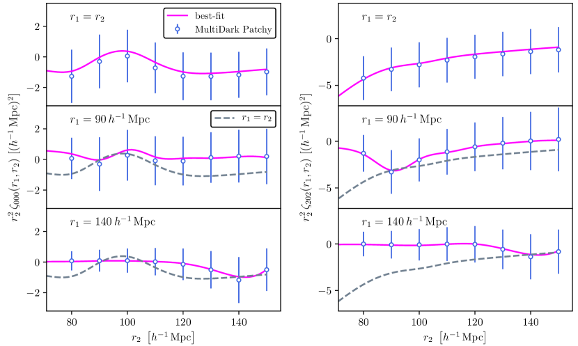
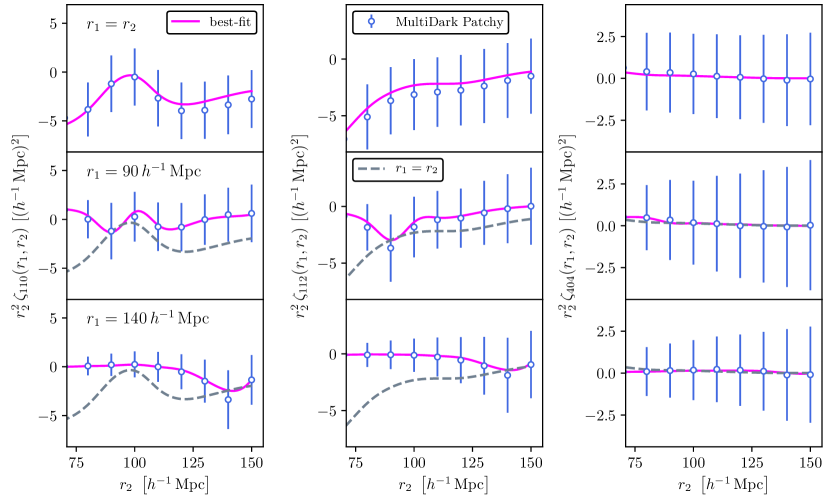
Figure 3 shows the theoretical predictions of the four bispectrum multipoles , , and as a function of , focusing only on the elements; , , , and shown in the figure are computed in the high- limit, and the sum of all of them reproduces the tree-level solution. The scale at which the terms including the mode-coupling integral dominate, i.e., the point at which the theoretical curves of and intersect, is for , for , for and for . The contribution of the , which consists of only the mode-coupling integral, is for , for , for and for up to . These results indicate that the contributions from the mode-coupling integrals to and are less than to and , and therefore, and are easier to predict than and . Sugiyama et al. (2019) showed that and have a higher signal-to-noise ratio than and , which suggests that and should be taken into account first when analyzing the bispectrum (or 3PCF). Note that both the and terms diverge, because they are proportional to and at small scales, respectively, as shown in Eqs. (55) and (56), and in Figure 3. However, the sum of them, , completely cancels out the divergence term (see orange lines in Figure 3.):
| (59) |
3.5 Template model
Now, we are ready to present a template model for the redshift-space bispectrum that explains the nonlinear degradation of the BAO signal. We start with the power spectrum case and show how to reproduce the power spectrum template model proposed by Eisenstein et al. (2007a) in the context of the IR cancellation. We then extend it to the bispectrum case.
The mode-coupling term is known to have a suppressed BAO signal compared to the linear power spectrum (Crocce & Scoccimarro, 2008). Nevertheless, the mode-coupling term arising from the IR flow is proportional to (47) and has the original BAO signal. This discrepancy is due to the assumption in Eq. (46), which corresponds to the assumption that the IR flow is uncorrelated with the density perturbation, as discussed in Section 3.2.
We propose an empirical method for breaking the IR cancellation and achieving physical effects. It is simply to replace appearing in the mode-coupling term (47) with (Eisenstein & Hu, 1998) that does not have the BAO signal:
| (60) |
Then, we obtain Eisenstein et al. (2007a)’s template
| (61) | |||||
where
| (62) |
Despite its simplicity, Eq. (61) provides highly unbiased constraints on the BAO signal and has passed various tests using high-precision -body simulations (e.g., Seo et al., 2008; Kim et al., 2009; Seo et al., 2010; Ross et al., 2017).
In a similar manner, we replace appearing in (53), (54), (55)and (56) with , resulting in
| (63) |
The above expression is one of the main results in this paper 222Blas et al. (2016) presented a bispectrum model for explaining the nonlinear BAO damping using an IR re-summation method in the context of the time-sliced perturbation theory. They performed the calculations for the case of dark matter in real space, and derived the term consisting of a product of and in the third line of Eq. (63).. The validity of this model will be examined in detail in Section 6 by comparing the theoretical predictions of the 3PCF using this model to the corresponding measurements from the mock catalogues.
4 Three-point correlation functions
4.1 Predictions of 3PCFs
As explained in the introduction, we adopt the 3PCF to analyze the data in order to extract all of the information from the BAO while keeping the number of data bins under control. The template model of the 3PCF for the data analysis is computed through the 2D Hankel transform (10) of the bispectrum template model given in Eq. (63).
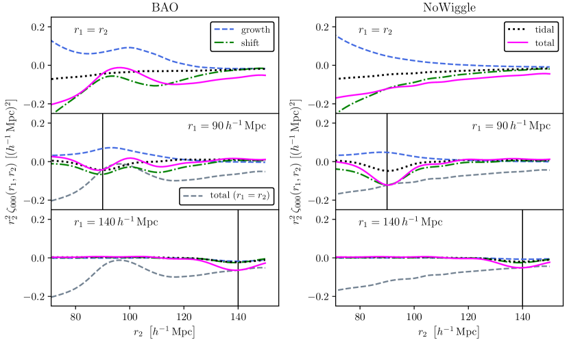
Here let us discuss the BAO information on the 3PCF, focusing on the impact of nonlinear gravity on the BAO signal. To this end, we focus on for dark matter in real space as the simplest example. We compare the theoretical predictions of our template model including BAO with those of the model without BAO, which consists of only , in Figure 4. In the no-wiggle case, the non-linearity arises from the second-order density perturbation of dark matter in real space only, and it can be decomposed into three sources, i.e., non-linear growth, shift effects, and tidal forces, as follows
| (64) | |||||
where the first, second and third terms represent the nonlinear growth, shift, and tidal force effects. In the figure, we investigate how those three components contribute to the final 3PCF. From the right panel of the figure, we find that in , in the range , the non-linear growth term is positive, and the shift and tidal force terms are negative. Since the total is negative, we can conclude that in this range, the shift and tidal force terms give the main contribution. In particular, from the middle and bottom right panels of the figure, we notice that at the point where , the shift and tidal force terms have a trough. We attribute this trough to the fact that the shift and tidal force terms arise from the spatial derivative of the density field, i.e., the relation between galaxies at different positions, and that thus the probability of finding a triplet of galaxies comprising the 3PCF at the same scale is reduced compared to the case. For the non-linear growth term, when the value at is positive or negative, it has a peak or trough, respectively. Thus, when we fix to , we find a peak; when we fix to , a trough appears, but this effect is too small to be visible in the figure.
In the case with BAO, we find the BAO signal around in the top left panel where is satisfied. However, in the middle left panel, the BAO peak at and the trough at cancel each other out and neither signal is clearly visible. On the scale where the BAO signal does not appear, i.e., in the bottom left panel (), we find an trough at as in the no-wiggle case.
4.2 Window function effects
Our estimator for measuring the 3PCF as shown in Section 6.1 requires to take into account how the survey geometry affects the measurement of 3PCFs. Following Sugiyama et al. (2019), we include the window function effect into the 3PCF model as follows
| (65) | |||||
where denotes the theoretical model corresponding the observed 3PCF multipoles, the bracket with multipole indices, , denotes the Wigner-j symbol, and is the 3PCF of the window function expanded in the TripoSH formalism. Throughout this paper, we ignore the contribution from the integral constraint (Peacock & Nicholson, 1991). This relation describes simply mixing of different multipole components, (), due to the survey window function. In practice we have one issue in calculating a 3PCF model that includes the effects of the window function in this method. As for the indexes corresponding to the LOS direction, and , due to RSD, one would expect that their contributions become smaller for larger and . However, for , , and corresponding to expansion w.r.t. and , it is not clear at which multipoles we should truncate to obtain a converged 3PCF. For this reason, let us examine below in detail the contributions of each multipole component. As a caveat, the results derived here correspond to the BOSS survey region, and a similar study is needed for each survey region in which the 3PCF is measured.
One may wonder why the survey window function correction is required for 3PCF measurements, i.e., in configuration space rather than Fourier space. We summarize key points here, leaving more elaborated discussions with some equations in Appendix A. In general, as long as we measure the multipole components of the 3PCF of galaxies, we have to take the survey window function of the 3PCF into account. Note that this fact is independent of whether we use FFTs to measure the 3PCF (Scoccimarro, 2015; Slepian & Eisenstein, 2016; Sugiyama et al., 2019), or not (Slepian & Eisenstein, 2015). We use FFTs for measuring the 3PCF, but if we only consider the monopole components of and , Eq. (65) matches Eq. (32) in Slepian & Eisenstein (2015), which is a measurement of 3PCF without FFTs, as already pointed out by Sugiyama et al. (2019). The difference from the treatment of the window function in Slepian & Eisenstein (2015) is that we convolve the window function in our theoretical model of the 3PCF, whereas Slepian & Eisenstein (2015) treats the multipole components of the 3PCF of the window function as a single matrix A and multiplies the measured multipole components of the 3PCF by its inverse matrix .
We propose one way to quantitatively assess the effect of the survey geometry. As can be seen from Figures 9 and 9, 3PCFs may change sign at large scales, i.e., 3PCFs may pass through a point with zero. In this case, for example, the calculation of the relative change diverges, making it difficult to interpret the results. Therefore, instead of checking for convergence in each (, )-bin, we calculate the 3PCFs averaged over a range of , which is used in the analysis of this paper (see Sections 5 and 6), and check whether the average values are converged: we compute
| (66) |
where is the number of data bins, which is for and for because we adopt a bin width of .
To estimate the extent to which other multipole components affect the multipole component of interest , we define the following quantities from Eq. (65):
| (67) | |||||
where means the same calculation manner as Eq. (66), and satisfies . In a similar manner, we also define the following quantities to find out which multipole components of the window function 3PCF are required:
| (68) | |||||
where . Note that the multipole indeces and associate with the theoretical model of the 3PCF, , and the window 3PCF, , respectively.
To compute and , we consider multipole components for monopole , for quadrupole , for hexadecapole () and for the tetrahexacontapole (), for a total of components. The specific multipole components that we calculate and their values for the NGC and SGC are summarized in Tables 1 and 2, where the absence or presence of round brackets represents the NGC or SGC results, respectively. The terms that contribute more than to the final results are highlighted in bold letters, and in this paper, we will include only such terms in the data analysis. These tables show that the contribution of the higher-order multipole components gradually decreases as the higher order is reached. This result allows us to conclude that we can use the expansion formalism of Eq. (65) with multipole components truncated at a finite order. The lower-order components of the quadrupole components such as and , are more important than the higher-order multipole components of the monopole components such as and . Unless we focus on the measurement of the hexadecapole, we do not need a theoretical model and a window function of the hexadecapole. As for the tetrahexacontapole (), we can ignore it for all the cases we are interested in. The contribution of each multipole component other than the multipole component of interest can be positive or negative, and the total contribution is - for , , and in both the NGC and SGC cases. For , the window function has a large effect of roughly , so the convergence of Eq. (65) is poor. For this reason, the results of may not have converged with just the components that we have consider in Tables 1 and 2. We include in our analysis with this caution; in Section 6, however, we find that does not have a significant contribution to our cosmological constraints at least in our setting.
We have further investigated the window function effect for the case of , even though we have not shown the results in Tables 1 and 2. The results are completely dominated by the effects of lower order multipole components rather than , and have not converged at all with the components that we have calculated here. This fact makes it difficult to use for cosmological analysis, but implies at the same time that there is little cosmological information in .
| monopole () | |||||
|---|---|---|---|---|---|
| 94.94 (90.02) | 2.16 (2.99) | -3.25 (-2.09) | 2.75 (1.80) | -2.74 (-3.88) | |
| 9.33 (12.60) | 103.22 (100.94) | 3.81 (2.65) | -8.74 (-5.55) | 1.96 (2.03) | |
| -0.02 (-0.05) | -0.56 (-0.77) | 2.31 (1.52) | 0.03 (-0.02) | 0.90 (0.95) | |
| 0.07 (0.11) | 0.05 (0.07) | 0.14 (0.06) | 0.02 (0.00) | -0.68 (-0.79) | |
| 0.01 (0.01) | -0.01 (-0.02) | 0.05 (0.03) | 0.02 (-0.00) | 1.62 (2.29) | |
| -0.02 (-0.03) | -0.02 (-0.04) | 0.02 (0.02) | 0.01 (-0.00) | 0.18 (0.29) | |
| -0.03 (-0.04) | -0.03 (-0.05) | 0.02 (-0.00) | -0.00 (0.00) | 0.00 (0.00) | |
| -0.02 (-0.03) | -0.02 (-0.04) | -0.00 (-0.00) | -0.00 (-0.00) | 0.00 (0.00) | |
| -0.02 (-0.03) | -0.02 (-0.02) | -0.00 (-0.00) | -0.00 (-0.00) | 0.00 (0.00) | |
| quadrupole () | |||||
| -4.51 (-2.74) | 1.16 (0.78) | 0.76 (0.83) | 3.28 (3.61) | 0.75 (0.81) | |
| 5.08 (3.33) | -3.76 (-2.45) | 5.02 (5.69) | 97.83 (93.54) | 1.78 (1.36) | |
| -4.00 (-2.44) | 0.93 (0.63) | 84.57 (83.32) | 2.64 (2.90) | 14.49 (9.00) | |
| -0.28 (-0.16) | -2.02 (-1.29) | 0.10 (0.18) | 0.38 (0.81) | -0.71 (-0.79) | |
| 0.10 (0.00) | 0.29 (0.18) | 0.04 (0.10) | 0.43 (0.69) | -0.27 (-0.32) | |
| -0.12 (-0.07) | -0.93 (-0.58) | 2.81 (3.69) | 0.23 (0.46) | -9.34 (-7.13) | |
| -0.10 (-0.08) | -0.20 (-0.12) | 0.72 (0.90) | 0.35 (0.52) | 0.55 (0.53) | |
| 0.06 (0.00) | 0.07 (-0.00) | 0.05 (0.12) | 0.09 (0.19) | 0.12 (0.16) | |
| -0.10 (-0.06) | -0.17 (-0.09) | 0.76 (1.09) | 0.23 (0.34) | 20.00 (15.27) | |
| -0.06 (-0.03) | -0.05 (-0.04) | 0.11 (0.15) | 0.17 (0.23) | -0.10 (-0.12) | |
| 0.02 (-0.01) | 0.02 (-0.00) | 0.02 (0.04) | 0.05 (0.09) | -0.16 (-0.21) | |
| -0.05 (-0.02) | -0.05 (-0.03) | 0.32 (0.48) | 0.11 (0.16) | 0.85 (0.46) | |
| -0.03 (-0.01) | -0.02 (-0.02) | 0.06 (0.09) | 0.11 (0.15) | 0.57 (0.34) | |
| 0.01 (-0.01) | 0.01 (-0.00) | 0.01 (0.02) | 0.03 (0.05) | 0.03 (0.05) | |
| -0.03 (-0.00) | -0.02 (-0.01) | 0.17 (0.24) | 0.08 (0.11) | 0.33 (0.35) | |
| hexadecapole () | |||||
| -0.01 (-0.01) | 0.00 (0.00) | 0.04 (0.03) | 0.00 (0.00) | 0.03 (0.05) | |
| -0.02 (-0.02) | 0.03 (0.03) | 0.03 (0.02) | -0.12 (-0.07) | 0.05 (0.07) | |
| -0.10 (-0.11) | 0.05 (0.05) | 0.78 (0.49) | -0.43 (-0.27) | 0.51 (0.67) | |
| 0.08 (0.08) | -0.05 (-0.05) | -0.14 (-0.09) | 0.37 (0.22) | 1.02 (1.39) | |
| -0.17 (-0.21) | 0.03 (0.03) | 0.54 (0.31) | 0.06 (0.04) | 62.42 (70.86) | |
| -0.00 (-0.00) | -0.01 (-0.02) | -0.00 (-0.01) | 0.00 (-0.00) | 0.03 (0.05) | |
| -0.02 (-0.02) | -0.00 (0.00) | 0.06 (0.08) | 0.01 (0.02) | -0.02 (-0.04) | |
| 0.03 (0.04) | 0.01 (0.01) | -0.00 (-0.00) | 0.00 (-0.01) | 0.00 (-0.02) | |
| -0.01 (-0.01) | -0.00 (-0.00) | 0.04 (0.01) | 0.00 (0.01) | 1.97 (1.04) | |
| -0.01 (-0.02) | -0.07 (-0.09) | 0.05 (0.02) | 0.02 (-0.00) | 3.29 (4.89) | |
| tetrahexacontapole () | |||||
| 0.00 (0.00) | -0.00 (-0.00) | -0.00 (-0.00) | -0.00 (-0.00) | 0.00 (-0.00) | |
| -0.00 (-0.00) | 0.00 (0.00) | -0.00 (-0.00) | -0.00 (-0.00) | -0.00 (-0.00) | |
| -0.00 (-0.00) | 0.00 (0.00) | 0.01 (0.01) | -0.00 (-0.00) | 0.01 (0.01) | |
| 0.01 (0.00) | -0.00 (-0.00) | -0.00 (-0.01) | 0.01 (0.01) | 0.02 (0.01) | |
| -0.00 (-0.00) | 0.00 (0.00) | 0.01 (0.01) | -0.00 (-0.00) | 0.38 (0.28) | |
| -0.00 (-0.00) | 0.00 (0.00) | 0.00 (0.00) | -0.00 (-0.00) | 0.10 (0.07) | |
| -0.00 (-0.00) | 0.00 (0.00) | 0.00 (0.00) | 0.00 (0.00) | 0.05 (0.04) |
| monopole () | |||||
|---|---|---|---|---|---|
| 94.94 (90.02) | 102.60 (99.94) | 86.30 (84.07) | 101.29 (95.33) | 64.25 (72.02) | |
| 9.33 (12.60) | 1.58 (2.19) | 5.84 (8.14) | 4.50 (6.08) | 3.59 (5.72) | |
| -0.02 (-0.05) | 0.64 (1.03) | 1.00 (1.60) | 0.81 (1.25) | 0.09 (0.16) | |
| 0.07 (0.11) | -0.00 (-0.01) | 0.49 (0.77) | 0.58 (0.90) | -0.02 (-0.04) | |
| 0.01 (0.01) | 0.01 (0.01) | 0.32 (0.51) | 0.32 (0.49) | -0.02 (-0.04) | |
| -0.02 (-0.03) | -0.01 (-0.03) | 0.10 (0.16) | 0.20 (0.30) | 0.03 (0.05) | |
| -0.03 (-0.04) | -0.02 (-0.03) | 0.06 (0.09) | 0.01 (0.01) | 0.00 (0.00) | |
| -0.02 (-0.03) | -0.02 (-0.03) | -0.00 (-0.00) | -0.00 (-0.00) | 0.00 (0.00) | |
| -0.02 (-0.03) | -0.00 (-0.01) | -0.00 (-0.00) | -0.00 (-0.00) | 0.00 (0.00) | |
| quadrupole () | |||||
| -4.51 (-2.74) | -3.81 (-2.40) | 3.16 (1.99) | -6.96 (-4.28) | 23.87 (17.48) | |
| 5.08 (3.33) | 2.56 (1.70) | 6.49 (4.40) | 4.51 (2.92) | -8.67 (-6.62) | |
| -4.00 (-2.44) | -3.00 (-1.89) | -4.94 (-3.14) | -6.70 (-4.13) | 13.74 (9.86) | |
| -0.28 (-0.16) | -0.29 (-0.17) | 0.10 (0.04) | -0.18 (-0.10) | 1.36 (0.84) | |
| 0.10 (0.00) | 0.21 (0.00) | 0.12 (0.01) | 0.37 (0.01) | -0.85 (-0.01) | |
| -0.12 (-0.07) | -0.25 (-0.14) | -0.43 (-0.24) | 0.11 (0.04) | 1.22 (0.78) | |
| -0.10 (-0.08) | -0.07 (-0.05) | 0.04 (0.02) | -0.06 (-0.03) | 0.36 (0.23) | |
| 0.06 (0.00) | 0.05 (0.00) | 0.04 (-0.00) | 0.10 (0.01) | -0.35 (-0.04) | |
| -0.10 (-0.06) | -0.06 (-0.03) | 0.02 (0.00) | 0.03 (0.00) | 0.25 (0.18) | |
| -0.06 (-0.03) | -0.05 (-0.03) | 0.03 (0.01) | -0.03 (-0.01) | 0.00 (0.00) | |
| 0.02 (-0.01) | 0.02 (-0.01) | 0.02 (-0.01) | 0.03 (-0.01) | -0.13 (0.05) | |
| -0.05 (-0.02) | -0.05 (-0.02) | 0.00 (-0.01) | 0.01 (-0.01) | 0.17 (0.09) | |
| -0.03 (-0.01) | -0.01 (-0.00) | 0.01 (-0.00) | -0.01 (-0.00) | 0.00 (0.00) | |
| 0.01 (-0.01) | 0.00 (-0.00) | 0.00 (-0.00) | 0.01 (-0.01) | -0.02 (0.02) | |
| -0.03 (-0.00) | -0.01 (-0.00) | 0.00 (-0.00) | 0.01 (-0.01) | 0.13 (0.02) | |
| hexadecapole () | |||||
| -0.01 (-0.01) | -0.00 (-0.00) | 0.72 (0.89) | 0.49 (0.59) | 1.83 (2.62) | |
| -0.02 (-0.02) | -0.00 (-0.00) | -0.12 (-0.10) | -0.22 (-0.20) | -0.64 (-0.86) | |
| -0.10 (-0.11) | 0.01 (0.01) | 0.40 (0.45) | 0.63 (0.68) | 0.56 (0.59) | |
| 0.08 (0.08) | 0.08 (0.09) | -0.34 (-0.33) | -0.15 (-0.14) | 2.89 (3.14) | |
| -0.17 (-0.21) | -0.11 (-0.14) | 0.48 (0.60) | 0.17 (0.21) | -4.36 (-6.20) | |
| -0.00 (-0.00) | 0.00 (0.00) | 0.02 (0.03) | 0.02 (0.03) | 0.20 (0.32) | |
| -0.02 (-0.02) | -0.00 (-0.00) | -0.05 (-0.07) | -0.06 (-0.07) | -0.22 (-0.34) | |
| 0.03 (0.04) | 0.01 (0.01) | 0.11 (0.15) | 0.13 (0.17) | -0.22 (-0.34) | |
| -0.01 (-0.01) | 0.01 (0.01) | -0.02 (-0.02) | -0.02 (-0.03) | 0.02 (0.01) | |
| -0.01 (-0.02) | -0.01 (-0.01) | -0.01 (-0.01) | 0.02 (0.02) | -0.12 (-0.25) | |
| tetrahexacontapole () | |||||
| 0.00 (0.00) | 0.00 (0.00) | -0.00 (-0.00) | 0.00 (0.00) | 0.57 (0.34) | |
| -0.00 (-0.00) | 0.00 (0.00) | -0.01 (-0.01) | 0.00 (0.00) | -0.08 (-0.13) | |
| -0.00 (-0.00) | -0.00 (-0.00) | 0.01 (0.01) | -0.00 (-0.00) | 0.42 (0.43) | |
| 0.01 (0.00) | 0.00 (0.00) | -0.00 (-0.00) | -0.02 (-0.01) | -0.65 (-0.55) | |
| -0.00 (-0.00) | -0.00 (-0.00) | 0.02 (0.02) | 0.01 (0.01) | 0.29 (0.28) | |
| -0.00 (-0.00) | 0.00 (0.00) | -0.01 (-0.01) | -0.01 (-0.01) | -0.10 (-0.17) | |
| -0.00 (-0.00) | 0.00 (0.00) | 0.02 (0.01) | 0.03 (0.02) | 0.60 (0.34) |
4.3 Decomposition in terms of parameters
In this subsection, we describe how to compute practically the theoretical predictions of the 3PCF in a fast manner. Before showing our procedure, let us first discuss the computational cost to calculate the 3PCF from the bispectrum template model given in Eq. (63) through the two-dimensional (2D) Hankel transformation in Eq. (10). First of all, a triple integration is needed to calculate the bispectrum multipole component (6). In particular, to compute the Hankel transform, we need to compute the model of the bispectrum multipole over a wide range of wavenumbers . In this paper, we compute bins on the log-scale over the range . The 2D Hankel transform itself can be computed fast using the FFTLog algorithm (Hamilton, 2000). Furthermore, as explained in Section 4.2, when we compute the theoretical prediction of the 3PCF multipole component of interest after taking into account the window function effect, we have to compute about other multipole components as well. Thus, calculating one multipole component of the 3PCF, e.g., or , requires triple integrals, which is so computationally expensive that it is not well suited for a fitting analysis.
To speed up the calculation of the theoretical predictions for 3PCFs, we linearize the fitting parameters on which the 3PCF depends by making the following two assumptions. The first is to fix the shape of the linear matter power spectrum and its smooth version contained in the bispectrum template model to their prediction by a fiducial cosmological model introduced in the introduction. Second, we rewrite the two-dimensional damping function describing the nonlinear attenuation of the BAO, (43), as
| (69) |
and fix the radial and transverse smoothing parameters, and , to the linear theory predictions (43) or the best-fitting values (see Section 5.2). Under these two assumptions, the bispectrum template model depends on five free parameters
| (70) |
except for the AP parameters, which will be discussed in detail in Section 4.4. Then, we can represent the model with a linear combination of those parameters as coefficients:
| (71) |
where
| (72) |
and
| (73) |
with
| (74) |
Finally, we replace and appearing in Eq. (63) with and , where , and are computed using fixed fiducial cosmological parameters, and substitute Eq. (71) into Eq. (63). We can then pre-calculate all the other parts of the template model (63) except and create a table of the resulting data. All that is left to do is to load that table when we perform our cosmological analysis.
4.4 AP effects
| monopole () | |||||
|---|---|---|---|---|---|
| 103.17 (98.20) | -0.00 (-0.00) | -3.72 (3.48) | -0.00 (-0.00) | 0.33 (0.77) | |
| -0.00 (-0.00) | 103.20 (98.43) | -0.00 (-0.00) | -4.11 (3.73) | 0.00 (0.00) | |
| 0.20 (0.21) | -0.00 (-0.00) | 0.41 (-0.49) | -0.00 (-0.00) | -1.82 (-4.40) | |
| -0.00 (-0.00) | 0.10 (0.10) | -0.00 (-0.00) | -0.00 (-0.00) | 0.00 (0.00) | |
| -0.00 (-0.00) | -0.00 (-0.00) | -0.00 (-0.00) | -0.00 (-0.00) | 0.44 (0.93) | |
| -0.00 (-0.00) | -0.00 (-0.00) | -0.00 (-0.00) | -0.00 (-0.00) | 0.00 (0.00) | |
| -0.00 (-0.00) | -0.00 (-0.00) | -0.00 (-0.00) | -0.00 (-0.00) | 0.00 (0.00) | |
| -0.00 (-0.00) | -0.00 (-0.00) | -0.00 (-0.00) | -0.00 (-0.00) | 0.00 (0.00) | |
| -0.00 (-0.00) | -0.00 (-0.00) | -0.00 (-0.00) | -0.00 (-0.00) | 0.00 (0.00) | |
| quadrupole () | |||||
| 5.42 (-5.73) | -0.00 (-0.00) | 0.18 (0.18) | -0.00 (-0.00) | 0.00 (0.00) | |
| -0.00 (-0.00) | -1.73 (1.68) | -0.00 (-0.00) | 104.59 (96.62) | 0.00 (0.00) | |
| -9.30 (9.42) | -0.00 (-0.00) | 103.98 (97.26) | -0.00 (-0.00) | 43.73 (-99.18) | |
| -0.00 (-0.00) | 2.80 (-3.01) | -0.00 (-0.00) | 0.02 (0.64) | 0.00 (0.00) | |
| 0.10 (0.11) | -0.00 (-0.00) | 0.26 (-0.31) | -0.00 (-0.00) | -0.97 (-2.33) | |
| 0.00 (0.00) | -4.16 (4.25) | -0.00 (-0.00) | -0.84 (0.65) | 0.00 (0.00) | |
| 0.00 (0.00) | -0.00 (-0.00) | -0.11 (-0.11) | -0.00 (-0.00) | 0.00 (0.00) | |
| 0.00 (0.00) | 0.04 (0.06) | -0.00 (-0.00) | 0.03 (0.03) | 0.00 (0.00) | |
| 0.00 (0.00) | -0.00 (-0.00) | 0.13 (0.12) | -0.00 (-0.00) | -13.59 (33.13) | |
| 0.00 (0.00) | -0.00 (-0.00) | -0.00 (-0.00) | -0.00 (-0.00) | 0.00 (0.00) | |
| 0.00 (0.00) | -0.00 (-0.00) | -0.00 (-0.00) | -0.00 (-0.00) | 0.27 (0.65) | |
| 0.00 (0.00) | -0.00 (-0.00) | -0.00 (-0.00) | -0.00 (-0.00) | 0.00 (0.00) | |
| 0.00 (0.00) | -0.00 (-0.00) | -0.00 (-0.00) | -0.00 (-0.00) | 0.00 (0.00) | |
| 0.00 (0.00) | -0.00 (-0.00) | -0.00 (-0.00) | -0.00 (-0.00) | 0.00 (0.00) | |
| 0.00 (0.00) | -0.00 (-0.00) | -0.00 (-0.00) | -0.00 (-0.00) | 0.01 (0.08) | |
| hexadecapole () | |||||
| -0.06 (-0.06) | -0.00 (-0.00) | -0.00 (-0.00) | -0.00 (-0.00) | 0.00 (0.00) | |
| -0.00 (-0.00) | 0.00 (0.00) | -0.00 (-0.00) | 0.04 (-0.07) | 0.00 (0.00) | |
| 0.02 (0.02) | -0.00 (-0.00) | -0.19 (0.17) | -0.00 (-0.00) | -0.26 (-0.62) | |
| -0.00 (-0.00) | 0.01 (0.01) | -0.00 (-0.00) | -1.19 (1.14) | 0.00 (0.00) | |
| 0.06 (0.06) | -0.00 (-0.00) | -1.11 (1.06) | -0.00 (-0.00) | 76.00 (161.08) | |
| -0.00 (-0.00) | -0.04 (-0.04) | -0.00 (-0.00) | -0.00 (-0.00) | 0.00 (0.00) | |
| -0.00 (-0.00) | -0.00 (-0.00) | -0.01 (-0.01) | -0.00 (-0.00) | 0.00 (0.00) | |
| -0.00 (-0.00) | 0.01 (0.01) | -0.00 (-0.00) | 0.01 (0.01) | 0.00 (0.00) | |
| -0.00 (-0.00) | -0.00 (-0.00) | 0.01 (0.01) | -0.00 (-0.00) | -2.17 (5.18) | |
| -0.00 (-0.00) | 0.03 (0.03) | -0.00 (-0.00) | -0.00 (-0.00) | 0.00 (0.00) | |
| tetrahexacontapole () | |||||
| -0.00 (-0.00) | -0.00 (-0.00) | -0.00 (-0.00) | -0.00 (-0.00) | 0.00 (0.00) | |
| -0.00 (-0.00) | -0.00 (-0.00) | -0.00 (-0.00) | -0.00 (-0.00) | 0.00 (0.00) | |
| -0.00 (-0.00) | -0.00 (-0.00) | -0.00 (-0.00) | -0.00 (-0.00) | 0.00 (0.00) | |
| -0.00 (-0.00) | -0.00 (-0.00) | -0.00 (-0.00) | 0.00 (0.00) | 0.00 (0.00) | |
| -0.00 (-0.00) | -0.00 (-0.00) | 0.00 (0.00) | -0.00 (-0.00) | -0.32 (0.77) | |
| -0.00 (-0.00) | -0.00 (-0.00) | -0.00 (-0.00) | 0.00 (0.00) | 0.00 (0.00) | |
| -0.00 (-0.00) | -0.00 (-0.00) | 0.00 (0.00) | -0.00 (-0.00) | -0.17 (0.33) |
In this section, we present a fast method for calculating the 3PCF changes due to the AP effect, which is caused by the use of incorrect cosmological parameters that are different from the true ones when calculating the distance to the galaxy from the measured redshift of the galaxy. In other words, the scale dependence of the theoretical model must be rescaled to compare the theoretical model calculated using the true cosmological parameters with the measurement with the wrong cosmological parameters. In particular, the anisotropic component of the AP effect gives rise to an additional angular dependence of the LOS direction, so the triple integral in Eq. (6) have to be recalculated each time in order to calculate the change of the bispectrum or 3PCF multipole component due to the AP effect. This fact makes it unsuitable for the method proposed in Section 4.3, which involves pre-building a table of the results of the 3PCF calculation. Therefore, we need to come up with a new approximation method to account for the anisotropic component of the AP effect.
To characterize the difference between the true and fiducial values of three-space coordinates (wavevectors), we usually introduce the following two AP parameters:
| (75) |
where and are the angular diameter distance and the Hubble parameter estimated at redshift in the observed region, respectively, and the subscript “fid” stands for “fiducial”. As an alternative parameterization of geometric distortions, we employ isotropic dilation and anisotropic warping parameters, defined as (Padmanabhan & White, 2008)
| (76) |
Using and , the true wavevector is represented as
| (77) |
and therefore, the corresponding wavenumber is given by
| (78) |
We then obtain the multipole components of the bispectrum, which contains the AP effect:
| (79) | |||||
where the pre-factor are because the bispectrum have dimensions of the square of the survey volume .
In the following, we explain how to compute the bispectrum multipoles, including the anisotropic warping of the AP effect, in a fast approximation. First, we decompose the true wavenumber into
| (80) |
where
| (81) |
Thus, as well as rescale wavenumber in , and also generates an additional angular-dependence of the LOS direction through . Second, we expand in TripoSHs with and as variables,
| (82) | |||||
where . Third, we expand around the point and obtain
| (83) | |||||
where
| (84) |
Finally, substituting Eqs. (82) and (83) into Eq. (79) leads to
| (85) | |||||
where
| (86) | |||||
The function depends only on and not on any other cosmological parameter. Therefore, it is possible to compute a function in various values of and create a table of data for it beforehand; can be expanded on the cosmological parameters, as described in Section 4.3, and a table of data can also be created by precomputing the parts of the function that do not depend on the cosmological parameters. This approximation method thus allows us to precompute all the functions needed for data analysis. When we actually analyze the data, we read these tables and use a numerical interpolation method to map them to any value.
Through the 2D Hankel transform (10), we derive the 3PCF multipoles including the AP effect:
| (87) | |||||
where
| (88) | |||||
| (89) |
and
| (90) | |||||
To investigate the convergence of the expansion of Eq. (87), we first calculate the average value of in the range , as in Eq. (66).
| (91) |
Here, is obtained by calculating the angle integral in Eq. (79) directly and does not use the approximation for the calculation of the AP effect described above. Next, as in Eq. (67), we define the following quantities
| (92) | |||||
where . We restrict the values of and that we calculate to . That is, we only calculate up to the first derivative of the bispectrum with respect to or , because it is difficult to calculate the higher derivative of the bispectrum with high precision by numerical calculations. Recall that the effect of multipole components other than the measured multipole component, which appears through the effect of the window function, is roughly - (Section 4.2). Therefore, we will only investigate the AP effect in detail for , , , and , which are the focus of our attention in this paper, and for other components, such as , , , and etc., we will simply consider the effect of the isotropic rescaling of the relative distance: .
Table 3 summarizes the contribution of the other multipolar components appearing through the anisotropic AP effect to the 3PCF multipole component of interest for and . Terms that contribute more than to the final results are written in bold, and we use only these bolded terms in our data analysis in Section 6. Each multipole component can be positive or negative, and the total contribution to , , or is less than . is more susceptible to the anisotropic AP effect, with for and for .
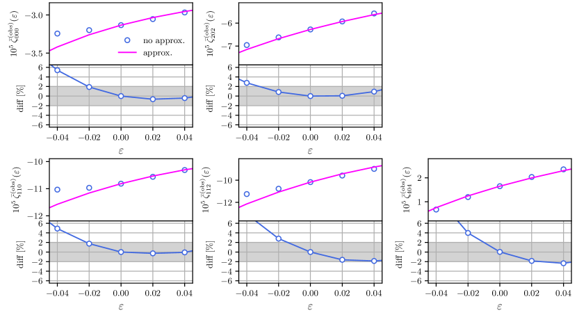
To check the validity of the approximation of our AP effect calculations in Eq. (87), Figure 5 plots (see Eq. (66)) as a function of . Note that, in this figure, the result shown is after accounting for the effect of the window function; therefore, this result is valid for a calculation in our actual data analysis. From this figure, we find that in the range , our approximation holds for , , and with a precision of . Since the standard deviation of estimated by the 2PCF, using the BOSS data we use in this paper, is for pre-reconstruction and for post-reconstruction (Ross et al., 2017; Beutler et al., 2017a), it is enough to consider the range . It is difficult to estimate the extent to which the uncertainty of a few percent in our approximation method will bias the final AP parameter estimates. Therefore, we will test the validity of this approximation by showing that it returns unbiased estimates of and in the data even for the case of and in Section 6.7.
5 2PCF analysis
The BAO and AP analysis in 2PCF is well established particularly for the BOSS survey (Ross et al., 2017; Beutler et al., 2017a; Gil-Marín et al., 2020). Nonetheless, in this section we summarize our 2PCF analysis, because we adopt a FFT-based multipole 2PCF estimator for a consistency with the 3PCF estimator. In short, we will show that our 2PCF analysis is consistent with previous studies, and hence readers interested in the joint analysis with 3PCF may skip to the next section.
5.1 Data
We use the MultiDark-Patchy mock catalogues (MD-Patchy mocks; Klypin et al., 2016; Kitaura et al., 2016), which are designed to reproduce the BOSS dataset. These mocks have been calibrated to a -body based reference sample using approximate gravity solvers and analytical-statistical biasing models and incorporate observational effects including the survey geometry, veto mask, and fiber collisions. The BOSS survey spans in two distinct sky regions (North and South Galactic Caps, hereafter NGC and SGC) in three redshift bins (, , and ). In this paper, we only use the middle redshift range, (), for both NGC and SGC. The fiducial cosmology for these mocks assumes a CDM cosmology given at the end of the introduction.
5.2 Methodology for 2PCF analysis
The fitting range we use for our analysis is . The bin width is for the 2PCF, and the number of bins in each multipole 2PCF is . Specifically, when we use and , the total number of bins is , and when we use , and , the total number of bins is .
When focusing only on large scales, such as , we expect Eisenstein et al. (2007a)’s template model (61) to be available to fit the 2PCF measurements, without the need for any nuisance parameters to reproduce the shape of the 2PCF at small scales. The validity of our expectations will be tested in Section 5.4. Then, the theoretical prediction of the 2PCF depends on the Kaiser factor (Kaiser, 1987) and the AP effect. Given that the galaxies in the NGC and SGC follow slightly different selections (Alam et al., 2017), we use two separate linear bias parameters to describe the clustering amplitude in the two samples: and . For the pre-reconstruction case, we compute and using the Zel’dovich approximation (Zel’Dovich, 1970) and fix them. For the post-reconstruction case, we find the best-fitting values of and by fixing , , , and to the best-fit values estimated for the pre-reconstruction case, resulting in and (for details of reconstruction, see Section 5.3). Note that the and values for post-reconstruction are larger than the expected values from the PT calculations (Seo et al., 2016). Beutler et al. (2017a) pointed out that this excess damping is because the MultiDark Patchy mocks tend to underestimate the BAO signal due to a limitation of the 2LPT approximation used in the mock production (for more details about the MultiDark-Patchy mock production, see Kitaura et al. (2016)). As shown by previous studies (e.g., Ross et al., 2017; Beutler et al., 2017a), the exact choice for and does not affect our analysis. The approach explained above yields fitting parameters as follows:
We measure the 2PCF through the inverse Fourier transform of the power spectrum. We employ the Fast Fourier Transform (FFT)-based estimator suggested by Bianchi et al. (2015); Scoccimarro (2015); Hand et al. (2017); Sugiyama et al. (2018). This method requires multiple FFT operations with the computational complexity of for each FFT process, where is the number of cells in the three-dimensional (3D) Cartesian grid in which the galaxies are binned. The FFT-based estimator is significantly faster than a straightforward pair counting analysis that would result in for the 2PCF, where is the number of galaxies or random particles. We use a Triangular Shaped Cloud (TSC) method to assign galaxies to 3D grid cells and correct for the aliasing effect following Jing (2005). Each side of our grid is in size, which is well below the minimum scale we use for analysis ().
Specifically, let and be the numbers of data galaxies and random galaxies at x. and include observational systematic weights (Ross et al., 2012; Anderson et al., 2014; Reid et al., 2016) and the FKP weight (Feldman et al., 1994). and are the total numbers of weighted data and random galaxies, respectively. The survey volume is estimated by
| (93) |
The observed density fluctuation is given by
| (94) |
We compute the Fourier transform of weighted by a spherical harmonic function
| (95) |
and then, we derive the estimator of the multipole 2PCF as follows:
| (96) |
with
| (97) |
where is the number of included in each bin, and is the TSC mass assignment function (Hockney & Eastwood, 1988). We properly subtract the shot-noise term from before transforming to (e.g., see Beutler et al., 2017a).
For the same reason as we mentioned in our 3PCF case in Section 4.2, we need to take into account the survey window function in this multipole 2PCF estimator. To this end, we measure the 2PCF multipoles of survey window functions, denoted , by replacing by in Eqs. (94)-(96). The theoretical model taking the survey geometry effect into account is given by (Wilson et al., 2017)
| (98) |
where “model” means that this masked model will be compared with the measured estimator. In the summation on the right-hand-side, we ignore all multipole terms beyond the hexadecapole of their smallness.
We estimate the covariance matrix from the set of Patchy mock catalogues described in Section 5.1. The mean of each 2PCF multipole is given by
| (99) |
with being the number of mock catalogues. Then, we derive the covariance matrix of as follows
| (100) |
The elements of the matrix are given by with .
The covariance matrix C that is inferred from mock catalogues suffers from the noise due to the finite number of mocks, which propagates directly to increased uncertainties in cosmological parameters (Hartlap et al., 2007; Taylor et al., 2013; Dodelson & Schneider, 2013; Percival et al., 2014; Taylor & Joachimi, 2014). This effect is decomposed into two factors. First, the inverse covariance matrix, , provides a biased estimate of the true inverse covariance matrix. To correct for this bias we rescale the inverse covariance matrix as (Hartlap et al., 2007)
| (101) |
where is the number of data bins. (see also Sellentin & Heavens (2016) as a recent work.) Second, we propagate the error in the covariance matrix to the error on the estimated parameters; this is done by scaling the standard deviation for each parameter by (Percival et al., 2014)
| (102) |
where is the number of parameters, and
| (103) | |||||
| (104) |
We compute the following quantity in each analysis performed in Sections 5 and 6 to estimate how much the fact that the number of mock catalogues is finite affects the final results:
| (105) |
This scaling is derived under the assumption of a Gaussian error distribution, which is not strictly true in our dataset. Therefore, it is better to produce many mock catalogues to keep this correction factor small. When using and , , and when using , and , . Thus, as long as we focus on the 2PCF-only analysis, the correction of Eq. (105) increases the parameter variance by about , which is negligible. However, in the joint analysis with the 3PCF, the number of data bins increases significantly, making this correction even more important (see Section 6).
5.3 Reconstruction
Density field reconstruction (Eisenstein et al., 2007b; Padmanabhan et al., 2012) is designed to improve the signal-to-noise ratio of the BAO signature by partially cancelling the nonlinear effects of structure formation, i.e., by returning the information that leaks to the higher-order statistics of the galaxy distribution back to the two-point statistics (Schmittfull et al., 2015).
In this paper, we adopt the simplest reconstruction scheme. We compute the displacement vector using the observed density fluctuation,
| (106) |
where is the input linear bias parameter. We smooth the density field with a Gaussian filter of the form, , where we chose , which is close to the optimal smoothing scale given by the signal-to-noise ratio of the BOSS data (Xu et al., 2012; Burden et al., 2014; Vargas-Magaña et al., 2017; Seo et al., 2016). The positions of all galaxies are modified based on the estimated displacement field . This procedure leads to a shifted galaxy field, , and a shifted random field, :
| (107) |
The reconstructed density fluctuation, required for the 2PCF estimate, can be obtained in an analogous way to Eq. (94) and is given by
| (108) |
We do not remove linear RSDs. At large scales, our reconstruction does not affect the linear density perturbation except for the damping effect of BAO. Therefore, we do not need to change the theoretical model of the quadrupole and hexadecapole.
We compute the window function multipoles using . In principle, after reconstruction, is correlated with through . In this paper, however, we assume that they are uncorrelated. In other words, we use the same equation (98) as before reconstruction to correct for the window function effect. This assumption is the same as used in Beutler et al. (2017a).
5.4 Results
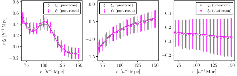
Figure 6 displays the measured pre- and post-reconstruction , and , from the MultiDark Patchy mock catalogues in the NGC for , and the associated best-fit model. We display the results for BAO fits on the mean of the MD-Patchy 2PCF multipoles in Table 4. The expected values of and are unity, and hence, and show how the estimated and from the analysis are biased. The standard deviations of and are denoted as and , respectively. is the correlation coefficient between and . We show (105) to clarify the impact on the effect due to the finite number of mocks to estimate the covariance matrix. We also fit each of individual mock catalogues and summarize the mean and standard deviation of the results in Table 5. The minimum statistics, denoted , is estimated for the best-fit parameters for each mock catalogue.
All of the four cases result in the values that are nearly unity and the -values that are larger than ; therefore, we conclude that the Eisenstein et al. (2007a)’s template model fits the measured Patchy 2PCF multipoles well at scales larger than . The results of the analysis are and for pre-reconstruction, and and for post-reconstruction, which are consistent with the results of the previous studies: e.g., compare our results with Table in Ross et al. 2017 or Table in Beutler et al. 2017a. The addition of the hexadecapole information reduces by for pre-reconstruction as shown by Taruya et al. (2011); Beutler et al. (2017b), while in the case of post-reconstruction, the addition of does not cause a significant improvement.
Tables 11 and 12 summarize our results of the constraints on . Since the expected value is , the bias of the estimated in our analysis is roughly of the - error. The - error in is before reconstruction and after reconstruction. As expected, the density field reconstruction decreases the errors in , with a reduction rate of about . In our analysis, the addition of does not change the results much.
According to previous studies, the error in using the monopole and quadrupole is for the 2PCF analysis (see Table 1 in Satpathy et al., 2017) and for the power spectrum analysis (see Table 2 in Beutler et al., 2017b). The power spectrum analysis also examines the addition of the hexadecapole, in which case the error in is reduced to . The reason why our constraint is weaker than the results of these previous studies is that our analysis uses only the large scales, , and our setup is such that the 2PCF extracts mostly the BAO-only information with a conservative estimate of .
6 Joint analysis with 3PCF
6.1 Methodology for 3PCF analysis
One of the major problems in the 3PCF analysis is the high degree of freedom, i.e., the large number of data bins. To reduce the number of data bins, we choose for the 3PCF measurements in the same scale range, , as used in the 2PCF analysis; the number of bins is then . For our decomposition formalism of the 3PCF, which is characterized by , the number of data bins is for and for .
Since we focus only on , we can directly use our template model given in Eq. (63), which is based on the tree-level solution with the nonlinear damping of BAO. We fix and to the same values used in the pre-reconstruction 2PCF analysis. We use two separate nonlinear bias parameters in the NGC and SGC samples: , , and . Thus, our 3PCF analysis uses fitting parameters as follows:
| (109) |
We employ the FFT-based estimator of the 3PCF suggested by Scoccimarro (2015); Slepian & Eisenstein (2016); Sugiyama et al. (2019). The setting of the FFT grids for the 3PCF measurements is the same as used for the 2PCF measurements. Specifically, the estimator of is given by (Section 4.3 in Sugiyama et al., 2019)
| (110) | |||||
where
| (111) |
Similar to the 2PCF case, we subtract the shot-noise term (Eq. (51) in Sugiyama et al., 2019) from the above estimator.
We have described in Section 4.2 how to compute a theoretical model of 3PCF that takes into account the effects of the window function.
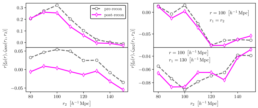
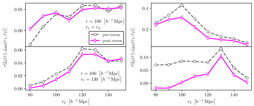
We follow the same manner to compute the mean and covariance matrix of mock 3PCF multipoles as used for the 2PCF analysis. Figure 7 displays the correlation coefficients between the 2PCF and 3PCF multipoles. Since the cross-covariance between the 2PCF and 3PCF arises from the non-linearity effect of gravity, we find that the correlation coefficient decrease as expected when reconstruction of the 2PCF is performed to partially remove the non-linear gravitational effect. Note that our reconstruction can mainly affect the isotropic component of the density field because it preserves linear RSDs (108). Therefore, and , which are dominated by monopole components, can be reduced, while and , which are dominated by quadrupole components, are virtually unchanged before and after the 2PCF reconstruction.
6.2 Results
| Patchy mock () | ||||||
| 0.003 | 0.026 | 0.000 | 0.061 | -0.49 | 1.012 | |
| (1) | 0.008 | 0.026 | -0.024 | 0.062 | -0.46 | 1.047 |
| (2) | 0.002 | 0.023 | -0.008 | 0.043 | -0.16 | 1.062 |
| (3) | 0.001 | 0.023 | -0.005 | 0.040 | -0.02 | 1.083 |
| (4) | 0.002 | 0.024 | -0.008 | 0.044 | -0.12 | 1.099 |
| (5) | 0.004 | 0.022 | 0.003 | 0.037 | -0.05 | 1.121 |
| 0.002 | 0.023 | 0.007 | 0.048 | -0.28 | 1.020 | |
| (6) | 0.002 | 0.024 | -0.003 | 0.049 | -0.28 | 1.055 |
| (7) | 0.001 | 0.023 | -0.003 | 0.040 | -0.06 | 1.071 |
| (8) | 0.001 | 0.023 | -0.002 | 0.038 | 0.07 | 1.091 |
| (9) | 0.000 | 0.024 | 0.000 | 0.040 | -0.03 | 1.108 |
| (10) | 0.000 | 0.023 | 0.000 | 0.037 | 0.08 | 1.130 |
| 0.006 | 0.017 | 0.006 | 0.033 | -0.44 | 1.012 | |
| (11) | 0.007 | 0.017 | -0.002 | 0.033 | -0.38 | 1.047 |
| (12) | 0.007 | 0.016 | 0.000 | 0.027 | -0.23 | 1.062 |
| (13) | 0.007 | 0.016 | 0.001 | 0.027 | -0.20 | 1.083 |
| (14) | 0.007 | 0.017 | -0.001 | 0.028 | -0.26 | 1.099 |
| (15) | 0.007 | 0.017 | 0.003 | 0.028 | -0.23 | 1.121 |
| 0.005 | 0.017 | 0.008 | 0.031 | -0.35 | 1.020 | |
| (16) | 0.007 | 0.017 | 0.003 | 0.032 | -0.30 | 1.055 |
| (17) | 0.006 | 0.016 | 0.003 | 0.027 | -0.18 | 1.071 |
| (18) | 0.006 | 0.016 | 0.004 | 0.027 | -0.15 | 1.091 |
| (19) | 0.006 | 0.016 | 0.005 | 0.027 | -0.18 | 1.108 |
| (20) | 0.006 | 0.017 | 0.003 | 0.027 | -0.16 | 1.130 |
| Patchy mock () | ||||||
|---|---|---|---|---|---|---|
| 0.003 | 0.0260.007 | -0.011 | 0.0610.020 | -0.480.05 | (55.510.5)/55 | |
| -0.001 | 0.0230.006 | -0.014 | 0.0430.010 | -0.160.19 | (239.923.3)/250 | |
| 0.001 | 0.0240.006 | 0.000 | 0.0490.015 | -0.290.08 | (84.212.0)/85 | |
| -0.002 | 0.0220.006 | -0.008 | 0.0390.009 | -0.080.19 | (265.423.2)/280 | |
| 0.004 | 0.0180.004 | 0.000 | 0.0350.008 | -0.450.037 | (53.210.1)/55 | |
| 0.004 | 0.0170.004 | -0.001 | 0.0280.007 | -0.280.121 | (238.922.8)/250 | |
| 0.002 | 0.0170.003 | 0.004 | 0.0320.006 | -0.360.070 | (83.813.0)/85 | |
| 0.003 | 0.0170.004 | 0.002 | 0.0270.006 | -0.230.16 | (266.423.0)/280 | |
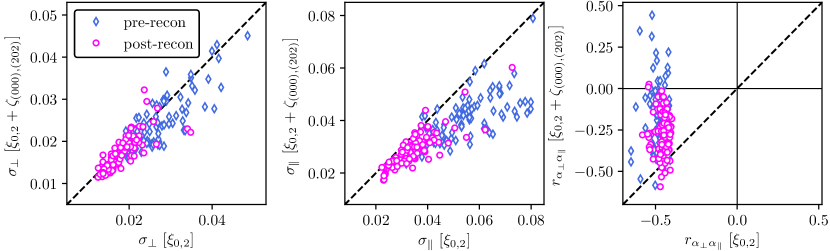
Figures 9 and 9 display , , , and measured from the MultiDark Patchy mock catalogues in the NGC for . Since the 3PCF multipoles depends on two scales, and , for display purposes, we plot them as a function of when fixing to , and , where we also show the associated best-fit models. For the BAO signal and non-linear gravitational effects found in in the case of real-space dark matter shown in Section 4.1, a similar behavior is observed even in the case of redshift-space galaxies. In the case of quadrupole components such as and , the BAO signal is largely suppressed by the non-linear effects of the bulk flow, so that only the effect of the trough at appears. Just to show how our best-fit model looks like at smaller scales, we leave Figures 13 and 13 in Appendix; they are the same as Figures 9 and 9, but extend the multipole components of the 3PCF at scales smaller than . We find that when and are both smaller than , the best-fit models start to deviate from the measurements from the mocks.
We present the results fitted to the mean of the MD-Patchy 2PCF multipoles in Table 4 and illustrate the results in Figure 14. We build on four 2PCF-only analyses presented in Section 5 and consider a joint analysis with the 3PCF multipoles in the following five cases. Hence in total we investigate cases, as labeled in Table 4 and Figure 14. First, let us consider the first and second terms of the monopole 3PCF. See cases (1), (6), (11) and (16). In all these four cases, we cannot find any improvement in the constraints on and compared to the 2PCF-only analysis. Next, let us consider the first terms of the monopole and quadrupole 3PCFs. See cases (2), (7), (12) and (17). We then find an improvement in constraints of , , and compared to the 2PCF analyses using , , and , respectively. With respect to constraints, only in case (2), we find an improvement compared to the corresponding 2PCF analysis. Note that after adding and , the results with and without hardly change. Finally, we add the second term of the quadrupole 3PCFs (), the first term of the hexadecapole 3PCFs (), or both of them to and . See cases (3)-(5), (8)-(10), (13)-(15) and (18)-(20). Even in all of these cases, we cannot find any significant change in the outcome. From these results, we conclude that the quadrupole 3PCFs are effective in constraining the Hubble parameter, and that a combination of data from , , and has the main information on the AP parameters. In the case of this minimum data set, the correction factor coming from the fact that we have a finite number of mocks to estimate the covariance matrix is , indicating that our covariance estimate is conservative. The 2D contours in the - plane for the and analyses are shown in Figure 15.
We fit each of individual mock catalogue when we add and to the 2PCF analysis and summarize the mean and standard deviation of the results in Table 5. All of the four cases result in the values that are nearly unity and the -values that are larger than , indicating that our template model (63) can explain the measured and well at . Considering the offset between our mean results and the fiducial value, i.e., and , the largest one for is in the analysis, less than of the standard deviation expected in these measurements. The bias in is larger than that in for pre-reconstruction, which is in the analysis. 2PCF reconstruction decreases the bias of and results in in the analysis, which is less than of the standard deviation.
We find that the addition of the isotropic and anisotropic 3PCFs ( and ) reduces the absolute value of by , , and compared to the original 2PCF analyses using , , and , respectively, while the 2PCF reconstruction does not significantly reduce , as shown in Table 5. In particular, before reconstruction, the value of is consistent with zero within the error. This fact means that we can treat the angular diameter distance and the Hubble parameter as mostly independent information to constrain cosmological parameters such as the equation of state of dark energy.
Figure 10 displays the uncertainties in and derived from the -only analysis vs. those from the joint analysis with and , recovered for each mock realization. This figure graphically confirms that the errors in and and the correlation coefficient between them tend to be reduced with the 3PCF for both pre- and post-reconstruction of the 2PCF. Specifically, the possibility that the information on and provides smaller errors in and is and , respectively.
In terms of derived parameters, we complement the results for and in Tables 9 and 10, and Figures 16 and 17. While the addition of the anisotropic 3PCF information does not improve the constraints on , there are , , and improvements for compared to the 2PCF analyses using , , and , respectively. After 2PCF reconstruction, even appears to show little improvement. Focusing on the correlation coefficient, , it is clearly less than half as much as the 2PCF results, similar to the case of .
Finally, we show in Tables 11 and 12 the results for , and the bias parameters. We do not find any improvement over the 2PCF results for , and even for , the constraints are weak. There are two possible reasons for the large errors in in particular: we focus only on large scales (), and is degenerate with the nonlinear bias parameters such as and .
6.3 Detection level of BAO
| Patchy mock () | |||||||
|---|---|---|---|---|---|---|---|
| (a) | -0.001 | 0.0650.017 | 0.007 | 0.1260.040 | -0.10 0.20 | (82.815.6)/55 | 27.310.6 |
| (b) | 0.003 | 0.0250.007 | -0.014 | 0.0480.013 | -0.19 0.17 | (243.123.9)/250 | 3.284.05 |
| (c) | -0.022 | 0.0610.009 | -0.054 | 0.0960.014 | 0.54 0.12 | (265.525.8)/250 | 25.711.1 |
| (d) | -0.004 | 0.0240.007 | -0.008 | 0.0370.009 | -0.110.22 | (242.123.1)/250 | 2.273.33 |
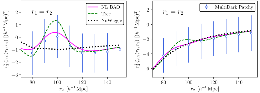
We discuss the detection level of the BAO signal. To do so, we analyze the dataset using each of the mock catalogues for the following three cases: (a) the 2PCF analysis using the no-wiggle 2PCF model, (b) the joint analysis using the non-linear BAO 2PCF model and the no-wiggle 3PCF model, and (c) the joint analysis using the no-wiggle 2PCF and 3PCF models. The results are summarized in Table 6. Using the no-wiggle 2PCF model, the constraints of and are and in case (a), and and in case (c), which are much weaker than in the results of Table 5 for both cases. This fact suggests that the BAO signal on the 2PCF makes a significant contribution to the constraint of the AP parameters, as has been well studied in the past. In case (b), where the no-wiggle model is used only for the 3PCF, the error in increases to , indicating that we loose constraining power by when we remove the BAO signal even on the 3PCF. In Figure 11, we find a clear difference between the no-wiggle 3PCF model and our non-linear BAO model. However, since case (b) results in a -value of , we cannot statistically reject the no-wiggle 3PCF model as long as we use the appropriate model for the 2PCF, which implies that we do not detect the BAO signal in the 3PCF with any high significance in our analysis.
To define the detection of the BAO signal, we calculate , which is the difference between the computed in our main analysis presented in Table 5 and those computed in cases (a), (b) and (c). Then, cases (a) to (c) results in statistical significances of , and , respectively, for the BAO detection. Our results show that the 3PCF contributes little to increasing the statistical significance for the BAO detection, and case (b) shows that the 3PCF alone can only yield a statistical significance of less than . As a reminder, in Section 6.2 we showed that for BOSS, including higher-order multipoles such as and did not increase the S/N of the BAO detection. This however might change for other datasets at different redshift. In addition, if one increases the number of multipole components to be considered, the value of (105) will increase. See Section 6.5 for a discussion of the impact of changes in the value on the results. From these results, we conclude that the reduction of (or ) errors by adding the 3PCF is not due to the BAO signal in the 3PCF, but rather to the effect of the shape of the anisotropic 3PCF.
6.4 Versus the tree-level solution
To demonstrate the validity of our template model (63), we compared our main result presented in Table 5 with the results of the analysis using the tree-level model. We have performed a joint analysis using the non-linear BAO 2PCF model and the tree-level 3PCF model, and the results are summarized as case (d) in Table 6. Figure 11 displays the best-fit tree-level 3PCF model. is calculated in the same way as in Section 6.3. The results show that the tree level model reduces the error in by compared to the results in Table 5 due to the emphasis on the BAO signal. If we assume that has a Gaussian distribution, the probability that our model gives a better fit, i.e., the probability that has a positive value, is . Based on these results, we conclude that it is safer to use our 3PCF model than using the tree-level solution, though as with the no-wiggle model, we cannot statistically reject the tree-level solution because the -value in case (d) is .
6.5 Number of mock realizations
| Patchy mock () | ||||||||
|---|---|---|---|---|---|---|---|---|
| [] | ||||||||
| 500 | 0.001 | 0.021 | -0.008 | 0.042 | -0.17 | 1.321 | ||
| 1000 | 0.004 | 0.022 | -0.005 | 0.042 | -0.09 | 1.137 | ||
| 1500 | 0.002 | 0.022 | -0.007 | 0.042 | -0.04 | 1.087 | ||
| 2048 | 0.007 | 0.023 | -0.011 | 0.040 | 0.053 | 1.218 | ||
We discuss the impact of changes in the number of the MD-Patchy mock catalogs on the results when estimating the covariance matrix. We compute three covariance matrices using , , and catalogs and then use them to analyze the data. We have performed an analysis using with bins, corresponding to case in Table 4. The results are summarized in Table 7 and illustrated in Figure 18. In this case, which has data bins, we find that if we use a number of mock catalogues, the error in is less than if we use catalogues. Thus, even using about times the number of catalogues as the number of data bins, the estimated error results are not fully converged. This fact indicates that for a more conservative analysis, it is important to keep the value of as close to as possible, as in our main result corresponding to 333Instead of the parameter, a more improved method to correct for the effect of a finite number of simulations have been proposed by (Sellentin & Heavens, 2016). This method requires fewer simulations and is expected to allow us to use higher multipole components safely..
6.6 A narrower bin size for 3PCFs
So far in this paper, we have used a wider bin size, , in our 3PCF analysis than used in our 2PCF analysis. Here, we show in Table 7 the results for the 3PCF analysis when we used the same bin size, i.e., , for the 3PCF analysis as for the 2PCF analysis. We have performed the same analysis as in case in Table 4, where we have used . In this case, the number of bins is and . With respect to , the error is reduced by about compared to the corresponding result in Table 4. However, we cannot determine whether this reduction in the error is the result of using the narrow bin width or whether it is due to the fact that the number of the mock catalogues is too small compared to the number of data bins. In the analysis using , the estimates of and return sufficiently low bias values, and the value of is also kept to a small value of . Therefore, to be conservative, we adopt the results in Tables 4 and 5 with as our main result.
6.7 Test of the AP effect
| Patchy mock () | ||||||
|---|---|---|---|---|---|---|
| 0.0045 | 0.0270.007 | 0.007 | 0.1100.063 | -0.40 0.08 | (54.410.6)/55 | |
| -0.0055 | 0.0240.006 | -0.011 | 0.0490.013 | -0.07 0.17 | (232.520.2)/250 | |
| 0.0031 | 0.0200.004 | -0.003 | 0.0420.014 | -0.43 0.03 | (55.29.1)/55 | |
| -0.0024 | 0.0190.004 | 0.001 | 0.0340.008 | -0.21 0.12 | (233.419.1)/250 | |
The previous analyses in this paper have verified that the estimated and return unity in measurements where no AP effect is present, i.e., where . In this subsection, we test whether the parameter estimation can correctly yield the expected values of and even when an AP effect is present, i.e., when and . This analysis is another validation of the approximate calculation of the anisotropy of the AP effect in the 3PCF given in Section 4.4.
We compute the radial distance to the galaxies using different cosmological parameters than those used to generate the Patchy mock catalogues and generate new 3D distributions of the galaxies. Specifically, we add the equation-of-state parameters for dark energy, and , to the fiducial parameters given in the introduction. In this case, the expected values of the AP parameters are and . For these newly created 3D galaxy catalogues, we repeat the same analysis as done in Table 5 and show the results in Table 8. The estimated biases of and are sufficiently small, e.g., less than of the standard deviation for the analysis using . This result validates the approximation method given in Section 4.4 to calculate the AP effect on the 3PCF. We therefore conclude that we can safely apply our analysis to actual observed galaxy data for which the AP parameters should not be 1.
7 Conclusions
We have established a joint analysis of anisotropic galaxy two- and three-point correlation functions (2PCF and 3PCF) in the range . Our analysis is based on a decomposition formalism of the 3PCF using tri-polar spherical harmonics (5). The reason why we have focused on the 3PCF instead of the bispectrum in Fourier space is that by looking only at scales larger than , it is possible to extract almost all of the BAO information that appears around . At such large scales, the non-linearity is weak, which simplifies the construction of the theoretical model of the 3PCF, and furthermore, the number of data bins required for analysis can be reduced. We apply density field reconstruction to the 2PCF measurement, but not in the 3PCF measurement. Specifically, we have (1) built a theoretical model of the bispectrum (3PCF) that incorporates the effects of BAO nonlinear damping (Section 3), (2) established an approximation to the fast computation of the theoretical model (Section 4), (3) applied our analysis method to the MultiDark Patchy mock catalogues to investigate which terms in the TripoSH expansion coefficients have the main cosmological information (Section 6.2), and (4) examined various systematic errors in our analysis, such as the comparison with the no-wiggle model (Section 6.3), the comparison with the tree-level solution (Section 6.4), the change in the number of mock realizations to estimate the covariance matrix (Section 6.5), the change in data bin size of the measured 3 PCF (Section 6.6), and the estimate of biases from the expected values of the AP parameters (Section 6.7). In particular, we highlight the result in Section 6.7, which confirms that the expected values of the AP parameters can be returned reliably even in the case of and , i.e., in the presence of the AP effect. In conclusion, we find that, in addition to the monopole and quadrupole components of the 2PCF ( and ), we can extract almost all the information for the angular diameter distance and the Hubble parameter by considering only the first terms of the monopole and quadrupole components of the 3PCF expanded using the TripoSH basis, i.e., and ; We have found the quadrupole component of the 3PCF to be particularly useful in constraining the Hubble parameter.
Our bispectrum model (63) is an analogy to the power spectrum model widely used in BAO analysis given by Eisenstein et al. (2007a). The shape of the bispectrum model is described by a tree-level solution consisting of no-wiggle power spectra with no BAO, while including the nonlinear damping of the BAO signature. The following three steps are required to build our bispectrum model. The first step is to expand the bispectrum using the -expansion according to Bernardeau et al. (2008) and classify it according to the structure of the mode-coupling integral (Section 3.3). The second step is to focus on the long-wavelength (infra-red) mode of flow of galaxies (IR flow) and to describe the non-linearity from the IR flow using the -expansion: in the limit where the IR flow is uncorrelated with the density perturbation, all the non-liniearities from the IR flow cancel each other out, resulting in the tree-level bispectrum (Sections 3.2 and 3.4). As the third step, we replace the linear power spectrum appearing in the mode-coupling terms of the bispectrum arising from the IR flow with no-wiggle power spectra without BAO (Section 3.5). These three operations yield the bispectrum model used in our analysis.
In describing the nonlinear terms arising from the IR flow using the -expansion, we can estimate the scale at which the mode-coupling terms begin to dominate in the bispectrum. It turns out that the mode-coupling terms start to become more important at larger scales for higher order multipole components such as and than for and , which are of particular interest to us in this paper (Figure 3). Thus, the model building would be much easier if one can show that it is sufficient to include and without the other higher multipole components.
A 2D Hankel transform (10) of the bispectrum model expanded in the TripoSH basis allows us to compute a theoretical model of the corresponding multipole components of the 3PCF. The TripoSH-expanded 3PCF is more attenuated at than at (the right panel in Figure 4). This is due to the terms called "shift" and "tidal force" in the second-order non-linear gravity (64). As expected, we find the BAO peak around in (top of the left panel in Figure 4). Interestingly, when we fix and plot as a function of , the trough at (which is more obvious in the right panel) closes in on the BAO peak at and the two partially cancel each other out and neither signal is clearly visible (middle of the left panel in Figure 4).
Since we measure the 3PCF using an FFT estimator presented by Sugiyama et al. (2019), we need to consider the effect of the survey geometry in the theoretical model in order to explain the results of our measurements. In the TripoSH expansion, a method to correct for the effect of the survey geometry on the 3PCF is given in Sugiyama et al. (2019). Although this method, in principle, requires an infinite number of multipole components to account for a single observed multipole component, we have tested the convergence of the expansion formalism in Eq. (65) for BOSS in this paper. To do so, we have considered several multipole components of the 3PCF: for monopole, for quadrupole, for hexadecapole, and for tetrahexacontapole, for a total of . For these components, we have calculated the theoretical model of the 3PCF and measured the window function 3PCF, respectively, to determine which multipole components contribute to the final result and to what extent. As a result, we have confirmed that the contribution tends to be smaller for higher order multipole components. In our analysis, we have decided to treat only the terms that contribute more than of these components (Tables 1 and 2).
In order to speed up the computation of the theoretical model of the 3PCF, we fix the shape of linear power spectra and the smoothing parameters, and (69), that describes the non-linear erasing of BAO. That is, we only vary parameters related to the amplitude of the 3PCF, such as , , and the bias parameters (, , and ). The 3PCF is then decomposed into terms (71) that depend only on the linear power spectrum, and . By calculating them in advance before analyzing the data, we can create a table of the resulting data and simply load the table when we perform the data analysis.
In order to quickly calculate the dependence of the anisotropic components of the AP parameters parameterized in (76) on the 3PCF, we expand the 3PCF with respect to (87). Then, by precomputing the terms that depend only on and creating a table of the resulting data, we can calculate the -dependence on the 3PCF by simply reading that table. We have confirmed that this approximation method can calculate the 3PCF multipoles of interest with an accuracy of in the range of (Figure 5).
We analyze both the pre- and post-reconstruction 2PCFs in the range . In this case, we use the template model of Eq. (61) for the theoretical calculation of the 2PCF without any nuisance parameter. This means that our analysis is in principle not a BAO analysis, but an RSD analysis. In particular, even though we only focus on large scales (), our analysis is the first rigorous RSD analysis to use the 2PCF after reconstruction. As for the constraints on the AP parameters (Table 5), our results using and measured from the MD-Patchy mock catalogues at have , and for pre-reconstruction, and , and for post-reconstruction, which are in good agreement with the previous studies of the BAO-only analysis (Ross et al., 2017; Beutler et al., 2017a). The results for (Table 12) are for pre-reconstruction and for post-reconstruction, which are weaker than in the previous studies of the full shape clustering (Satpathy et al., 2017; Beutler et al., 2017b), since we have only used large scales above ; after reconstruction, as expected, the error in is about smaller than the result before reconstruction.
We have measured five multipole components, , , , , and , and used them to perform a joint analysis with the 2PCF (Table 4). In the analysis of the 3PCF, we pay particular attention to the value of (105), a factor that compensates for the uncertainty in the estimated errors in parameters arising from the fact that the number of simulations used to measure the covariance matrix is finite, and we believe that the closer is to , the more conservative the analysis is. For this reason, we treat a minimum dataset as the main analysis of our paper, and we have confirmed that even adding other components such as and does not change the results significantly. In the main analysis, where the corresponding value is , the error in the Hubble parameter is better before the 2PCF reconstruction (i.e., ) and better after the 2PCF reconstruction (i.e., ) than the results using the 2PCF alone. Furthermore, the absolute value of the anti-correlation coefficient () between the angular diameter distance and the Hubble parameter is reduced by before the 2PCF reconstruction and after the 2PCF reconstruction. This is a major feature of adding the anisotropic 3PCF, considering that the with the pre- or post-reconstruction 2PCF alone remains near that is expected for the 2PCF BAO-only analysis. That is, adding 3PCF changes the degeneracy direction. Specifically, from the mean of the results from each independent mock catalogue (Table 5), we obtain , and before the 2PCF reconstruction, and , and after the 2PCF reconstruction. The constraint on the growth rate, (Table 12), does not improve at all compared to the results of our analysis using only the 2PCF. This is due to the fact that we only use large scales (). For similar reasons, the constraint, , obtained from the 3PCF is also very weak.
In our main analysis using , we have not detected the BAO signal in the 3PCF with any high significance: the statistical significance is . Therefore, we conclude that the reduction of the error in the Hubble parameter in our analysis is not due to the BAO signal in the 3PCF, but rather to the changes in the shape of and due to the anisotropic AP effect (Section 6.3).
The possibility that our template model (63) gives a better fit to the measurement than the tree-level model is ; if we use the tree-level model, the error in the Hubble parameter is reduced compared to our main result because of the emphasis on the BAO signal. Therefore, it is safer to use our model for a conservative analysis (Section 6.4). For future galaxy surveys, such as DESI, this difference in theoretical models should be more pronounced.
Table 7 and Figure 18 summarize the differences in results for different numbers of mock simulations to compute the covariance matrix. The number of data bins in our main analysis using is . We have found that using a number of simulations of e.g. underestimates the error in the diameter distance by , even after accounting for the correction by the factor (105). Similarly, the same table and figure summarize the results when the bin width of the 3PCF measurement has been decreased to and the number of data bins has been increased to . Then, we have found a reduction in the Hubble parameter error when using mock simulations compared to the results of our main analysis. We leave it to future work to find out if a similar reduction in the errors is seen when we increase the number of simulations beyond . As long as we only use mock catalogues, for a conservative analysis we propose to continue to use .
Finally, we have tested whether our analysis can correctly estimate the expected values of the angular diameter distance and the Hubble parameter in the presence of an AP effect, i.e., if and are not . To do so, we have measured the distance to the mock galaxies using the equation-of-state parameters for dark energy, and , to create a new 3D mock galaxy catalogues. The expected value of the AP parameters are then and . Our results (Table 8) show and for , and and for . Thus, for the joint analysis of the post-reconstruction 2PCF and the pre-reconstruction 3PCF, the biases in and are less than of the corresponding - errors. This test confirms the validity of applying our analysis method to real observed galaxy data, which should have and .
There are a variety of possible next research directions. The first and most obvious one is to apply our analysis method to actual observed galaxy data. The analysis of the 3PCF after reconstruction would also be straightforward. A conservative analysis of the 3PCF using up to small scales would require building a theoretical model of the 3PCF (or the bispectrum) to explain the observations and either increasing the number of mock simulations or calculating the covariance matrix of the 3PCF from an analytical approach (Sugiyama et al., 2020; Philcox & Eisenstein, 2019). We expect that our 3PCF analysis will also play a major role in the probe of primordial non-Gaussianity (Shirasaki et al., 2020).
Acknowledgements
NSS is grateful to Masato Shirasaki for very useful discussion. NSS acknowledges financial support from JSPS KAKENHI Grant Number 19K14703. Numerical computations were carried out on Cray XC50 at Center for Computational Astrophysics, National Astronomical Observatory of Japan. FB is a Royal Society University Research Fellow.
Data availability
The data underlying this article are available at the SDSS data base (https://www.sdss.org/dr12/).
References
- Alam et al. (2015) Alam S., et al., 2015, Astrophys. J. Suppl., 219, 12
- Alam et al. (2017) Alam S., et al., 2017, Mon. Not. Roy. Astron. Soc., 470, 2617
- Alcock & Paczyński (1979) Alcock C., Paczyński B., 1979, Nature, 281, 358
- Anderson et al. (2013) Anderson L., et al., 2013, Mon. Not. Roy. Astron. Soc., 427, 3435
- Anderson et al. (2014) Anderson L., et al., 2014, Mon. Not. Roy. Astron. Soc., 441, 24
- Audren et al. (2013) Audren B., Lesgourgues J., Benabed K., Prunet S., 2013, JCAP, 1302, 001
- Baldauf et al. (2012) Baldauf T., Seljak U., Desjacques V., McDonald P., 2012, Phys. Rev. D, 86, 083540
- Bernardeau et al. (2002) Bernardeau F., Colombi S., Gaztanaga E., Scoccimarro R., 2002, Phys. Rept., 367, 1
- Bernardeau et al. (2008) Bernardeau F., Crocce M., Scoccimarro R., 2008, Phys. Rev., D78, 103521
- Bernardeau et al. (2012) Bernardeau F., Crocce M., Scoccimarro R., 2012, Phys. Rev., D85, 123519
- Bertacca et al. (2018) Bertacca D., Raccanelli A., Bartolo N., Liguori M., Matarrese S., Verde L., 2018, Phys. Rev. D, 97, 023531
- Beutler et al. (2011) Beutler F., et al., 2011, Mon. Not. Roy. Astron. Soc., 416, 3017
- Beutler et al. (2017a) Beutler F., et al., 2017a, Mon. Not. Roy. Astron. Soc., 464, 3409
- Beutler et al. (2017b) Beutler F., et al., 2017b, Mon. Not. Roy. Astron. Soc., 466, 2242
- Bianchi et al. (2015) Bianchi D., Gil-Marín H., Ruggeri R., Percival W. J., 2015, Mon. Not. Roy. Astron. Soc., 453, L11
- Blake et al. (2011a) Blake C., et al., 2011a, Mon. Not. Roy. Astron. Soc., 415, 2892
- Blake et al. (2011b) Blake C., et al., 2011b, Mon. Not. Roy. Astron. Soc., 418, 1707
- Blas et al. (2011) Blas D., Lesgourgues J., Tram T., 2011, J. Cosmology Astropart. Phys., 2011, 034
- Blas et al. (2013) Blas D., Garny M., Konstandin T., 2013, JCAP, 1309, 024
- Blas et al. (2016) Blas D., Garny M., Ivanov M. M., Sibiryakov S., 2016, JCAP, 1607, 028
- Bolton et al. (2012) Bolton A. S., et al., 2012, Astron. J., 144, 144
- Brinckmann & Lesgourgues (2018) Brinckmann T., Lesgourgues J., 2018, arXiv e-prints, p. arXiv:1804.07261
- Burden et al. (2014) Burden A., Percival W. J., Manera M., Cuesta A. J., Magana M. V., Ho S., 2014, Mon. Not. Roy. Astron. Soc., 445, 3152
- Chiang & Slosar (2018) Chiang C.-T., Slosar A. z., 2018, JCAP, 07, 049
- Clarkson et al. (2019) Clarkson C., de Weerd E. M., Jolicoeur S., Maartens R., Umeh O., 2019, MNRAS, 486, L101
- Crocce & Scoccimarro (2006) Crocce M., Scoccimarro R., 2006, Phys. Rev., D73, 063519
- Crocce & Scoccimarro (2008) Crocce M., Scoccimarro R., 2008, Phys. Rev., D77, 023533
- Dawson et al. (2013) Dawson K. S., et al., 2013, Astron. J., 145, 10
- Desjacques et al. (2018) Desjacques V., Jeong D., Schmidt F., 2018, Phys. Rept., 733, 1
- Dodelson & Schneider (2013) Dodelson S., Schneider M. D., 2013, Phys. Rev., D88, 063537
- Eisenstein & Hu (1998) Eisenstein D. J., Hu W., 1998, Astrophys. J., 496, 605
- Eisenstein et al. (2001) Eisenstein D. J., et al., 2001, Astron. J., 122, 2267
- Eisenstein et al. (2005) Eisenstein D. J., et al., 2005, Astrophys. J., 633, 560
- Eisenstein et al. (2007a) Eisenstein D. J., Seo H.-j., White M. J., 2007a, Astrophys. J., 664, 660
- Eisenstein et al. (2007b) Eisenstein D. J., Seo H.-j., Sirko E., Spergel D., 2007b, Astrophys. J., 664, 675
- Eisenstein et al. (2011) Eisenstein D. J., et al., 2011, Astron. J., 142, 72
- Feldman et al. (1994) Feldman H. A., Kaiser N., Peacock J. A., 1994, Astrophys. J., 426, 23
- Gil-Marín et al. (2015) Gil-Marín H., Noreña J., Verde L., Percival W. J., Wagner C., Manera M., Schneider D. P., 2015, Mon. Not. Roy. Astron. Soc., 451, 539
- Gil-Marín et al. (2020) Gil-Marín H., et al., 2020, MNRAS, 498, 2492
- Gil-Marĺn et al. (2017) Gil-Marĺn H., Percival W. J., Verde L., Brownstein J. R., Chuang C.-H., Kitaura F.-S., Rodrlguez-Torres S. A., Olmstead M. D., 2017, Mon. Not. Roy. Astron. Soc., 465, 1757
- Gualdi & Verde (2020) Gualdi D., Verde L., 2020, JCAP, 06, 041
- Hahn et al. (2020) Hahn C., Villaescusa-Navarro F., Castorina E., Scoccimarro R., 2020, JCAP, 03, 040
- Hajian & Souradeep (2003) Hajian A., Souradeep T., 2003, Astrophys. J., 597, L5
- Hamilton (1997) Hamilton A. J. S., 1997, in Ringberg Workshop on Large Scale Structure Ringberg, Germany, September 23-28, 1996. (arXiv:astro-ph/9708102), doi:10.1007/978-94-011-4960-0_17
- Hamilton (2000) Hamilton A., 2000, Mon. Not. Roy. Astron. Soc., 312, 257
- Hand et al. (2017) Hand N., Li Y., Slepian Z., Seljak U., 2017, JCAP, 07, 002
- Hartlap et al. (2007) Hartlap J., Simon P., Schneider P., 2007, A&A, 464, 399
- Hockney & Eastwood (1988) Hockney R. W., Eastwood J. W., 1988, Computer Simulation Using Particles. CRC Press, PA, United States, https://ui.adsabs.harvard.edu/abs/1981csup.book.....H
- Jain & Bertschinger (1996) Jain B., Bertschinger E., 1996, Astrophys. J., 456, 43
- Jing (2005) Jing Y., 2005, Astrophys. J., 620, 559
- Kaiser (1987) Kaiser N., 1987, Mon. Not. Roy. Astron. Soc., 227, 1
- Kehagias & Riotto (2013) Kehagias A., Riotto A., 2013, Nucl. Phys., B873, 514
- Kim et al. (2009) Kim J., Park C., Gott III R., Dubinski J., 2009, Astrophys. J., 701, 1547
- Kitaura et al. (2016) Kitaura F.-S., et al., 2016, Mon. Not. Roy. Astron. Soc., 456, 4156
- Klypin et al. (2016) Klypin A., Yepes G., Gottlober S., Prada F., Hess S., 2016, Mon. Not. Roy. Astron. Soc., 457, 4340
- Landy & Szalay (1993) Landy S. D., Szalay A. S., 1993, Astrophys. J., 412, 64
- Laureijs et al. (2011) Laureijs R., et al., 2011, arXiv e-prints, p. arXiv:1110.3193
- Levi et al. (2013) Levi M., et al., 2013, preprint, (arXiv:1308.0847)
- Maartens et al. (2020) Maartens R., Jolicoeur S., Umeh O., De Weerd E. M., Clarkson C., Camera S., 2020, J. Cosmology Astropart. Phys., 2020, 065
- Makino et al. (1992) Makino N., Sasaki M., Suto Y., 1992, Phys. Rev., D46, 585
- Matsubara (1995) Matsubara T., 1995, Astrophys. J. Suppl., 101, 1
- Matsubara (2008a) Matsubara T., 2008a, Phys. Rev., D77, 063530
- Matsubara (2008b) Matsubara T., 2008b, Phys. Rev., D78, 083519
- Okumura et al. (2008) Okumura T., Matsubara T., Eisenstein D. J., Kayo I., Hikage C., Szalay A. S., Schneider D. P., 2008, Astrophys. J., 676, 889
- Padmanabhan & White (2008) Padmanabhan N., White M. J., 2008, Phys. Rev., D77, 123540
- Padmanabhan et al. (2012) Padmanabhan N., Xu X., Eisenstein D. J., Scalzo R., Cuesta A. J., Mehta K. T., Kazin E., 2012, Mon. Not. Roy. Astron. Soc., 427, 2132
- Pan & Szapudi (2005) Pan J., Szapudi I., 2005, Mon. Not. Roy. Astron. Soc., 362, 1363
- Peacock & Nicholson (1991) Peacock J. A., Nicholson D., 1991, MNRAS, 253, 307
- Pearson & Samushia (2018) Pearson D. W., Samushia L., 2018, Mon. Not. Roy. Astron. Soc., 478, 4500
- Peloso & Pietroni (2013) Peloso M., Pietroni M., 2013, JCAP, 1305, 031
- Peloso & Pietroni (2017) Peloso M., Pietroni M., 2017, JCAP, 1701, 056
- Percival et al. (2010) Percival W. J., et al., 2010, Mon. Not. Roy. Astron. Soc., 401, 2148
- Percival et al. (2014) Percival W. J., et al., 2014, Mon. Not. Roy. Astron. Soc., 439, 2531
- Philcox & Eisenstein (2019) Philcox O. H., Eisenstein D. J., 2019, Mon. Not. Roy. Astron. Soc., 490, 5931
- Reid et al. (2016) Reid B., et al., 2016, Mon. Not. Roy. Astron. Soc., 455, 1553
- Ross et al. (2012) Ross A. J., et al., 2012, Mon. Not. Roy. Astron. Soc., 424, 564
- Ross et al. (2015) Ross A. J., Samushia L., Howlett C., Percival W. J., Burden A., Manera M., 2015, Mon. Not. Roy. Astron. Soc., 449, 835
- Ross et al. (2017) Ross A. J., et al., 2017, Mon. Not. Roy. Astron. Soc., 464, 1168
- Saito et al. (2014) Saito S., Baldauf T., Vlah Z., Seljak U., Okumura T., McDonald P., 2014, Phys. Rev. D, 90, 123522
- Sánchez (2020) Sánchez A. G., 2020, Phys. Rev. D, 102, 123511
- Satpathy et al. (2017) Satpathy S., et al., 2017, Mon. Not. Roy. Astron. Soc., 469, 1369
- Schmittfull et al. (2015) Schmittfull M., Feng Y., Beutler F., Sherwin B., Chu M. Y., 2015, Phys. Rev. D, 92, 123522
- Scoccimarro (2015) Scoccimarro R., 2015, Phys. Rev. D, 92, 083532
- Scoccimarro & Frieman (1996) Scoccimarro R., Frieman J., 1996, Astrophys. J. Suppl., 105, 37
- Scoccimarro et al. (1999) Scoccimarro R., Couchman H. M. P., Frieman J. A., 1999, Astrophys. J., 517, 531
- Sellentin & Heavens (2016) Sellentin E., Heavens A. F., 2016, MNRAS, 456, L132
- Seo et al. (2008) Seo H.-J., Siegel E. R., Eisenstein D. J., White M., 2008, Astrophys. J., 686, 13
- Seo et al. (2010) Seo H.-J., et al., 2010, Astrophys. J., 720, 1650
- Seo et al. (2012) Seo H.-J., et al., 2012, Astrophys. J., 761, 13
- Seo et al. (2016) Seo H.-J., Beutler F., Ross A. J., Saito S., 2016, Mon. Not. Roy. Astron. Soc., 460, 2453
- Shiraishi et al. (2017) Shiraishi M., Sugiyama N. S., Okumura T., 2017, Phys. Rev., D95, 063508
- Shirasaki et al. (2020) Shirasaki M., Sugiyama N. S., Takahashi R., Kitaura F.-S., 2020, arXiv e-prints, p. arXiv:2010.04567
- Slepian & Eisenstein (2015) Slepian Z., Eisenstein D. J., 2015, Mon. Not. Roy. Astron. Soc., 454, 4142
- Slepian & Eisenstein (2016) Slepian Z., Eisenstein D. J., 2016, Mon. Not. Roy. Astron. Soc., 455, L31
- Slepian & Eisenstein (2017) Slepian Z., Eisenstein D. J., 2017, Mon. Not. Roy. Astron. Soc., 469, 2059
- Slepian & Eisenstein (2018) Slepian Z., Eisenstein D. J., 2018, MNRAS, 478, 1468
- Slepian et al. (2017) Slepian Z., et al., 2017, Mon. Not. Roy. Astron. Soc., 469, 1738
- Sugiyama (2014) Sugiyama N. S., 2014, Astrophys. J., 788, 63
- Sugiyama & Futamase (2012) Sugiyama N. S., Futamase T., 2012, Astrophys. J., 760, 114
- Sugiyama & Futamase (2013) Sugiyama N. S., Futamase T., 2013, Astrophys. J., 769, 106
- Sugiyama & Spergel (2014) Sugiyama N. S., Spergel D. N., 2014, JCAP, 1402, 042
- Sugiyama et al. (2018) Sugiyama N. S., Shiraishi M., Okumura T., 2018, Mon. Not. Roy. Astron. Soc., 473, 2737
- Sugiyama et al. (2019) Sugiyama N. S., Saito S., Beutler F., Seo H.-J., 2019, MNRAS, 484, 364
- Sugiyama et al. (2020) Sugiyama N. S., Saito S., Beutler F., Seo H.-J., 2020, MNRAS, 497, 1684
- Suto & Sasaki (1991) Suto Y., Sasaki M., 1991, Phys. Rev. Lett., 66, 264
- Szapudi (2004) Szapudi I., 2004, Astrophys. J., 605, L89
- Takada et al. (2014) Takada M., et al., 2014, PASJ, 66, R1
- Taruya et al. (2011) Taruya A., Saito S., Nishimichi T., 2011, Phys. Rev. D, 83, 103527
- Taylor & Hamilton (1996) Taylor A. N., Hamilton A. J. S., 1996, Mon. Not. Roy. Astron. Soc., 282, 767
- Taylor & Joachimi (2014) Taylor A., Joachimi B., 2014, Mon. Not. Roy. Astron. Soc., 442, 2728
- Taylor et al. (2013) Taylor A., Joachimi B., Kitching T., 2013, Mon. Not. Roy. Astron. Soc., 432, 1928
- Tegmark et al. (2006) Tegmark M., et al., 2006, Phys. Rev., D74, 123507
- Tojeiro et al. (2014) Tojeiro R., et al., 2014, Mon. Not. Roy. Astron. Soc., 440, 2222
- Vargas-Magaña et al. (2017) Vargas-Magaña M., Ho S., Fromenteau S., Cuesta A., 2017, Mon. Not. Roy. Astron. Soc., 467, 2331
- Varshalovich et al. (1988) Varshalovich D. A., Moskalev A. N., Khersonskii V. K., 1988, Quantum Theory of Angular Momentum. WORLD SCIENTIFIC, Singapore, doi:10.1142/0270
- Verde et al. (2000) Verde L., Heavens A. F., Matarrese S., 2000, Mon. Not. Roy. Astron. Soc., 318, 584
- Veropalumbo et al. (2016) Veropalumbo A., Marulli F., Moscardini L., Moresco M., Cimatti A., 2016, Mon. Not. Roy. Astron. Soc., 458, 1909
- Vishniac (1983) Vishniac E., 1983, Mon. Not. Roy. Astron. Soc., 203, 345
- White (2015) White M., 2015, MNRAS, 450, 3822
- Wilson et al. (2017) Wilson M. J., Peacock J. A., Taylor A. N., de la Torre S., 2017, Mon. Not. Roy. Astron. Soc., 464, 3121
- Xu et al. (2012) Xu X., Padmanabhan N., Eisenstein D. J., Mehta K. T., Cuesta A. J., 2012, Mon. Not. Roy. Astron. Soc., 427, 2146
- Xu et al. (2013) Xu X., Cuesta A. J., Padmanabhan N., Eisenstein D. J., McBride C. K., 2013, Mon. Not. Roy. Astron. Soc., 431, 2834
- Zel’Dovich (1970) Zel’Dovich Y. B., 1970, A&A, 500, 13
- Zhao et al. (2017) Zhao G.-B., et al., 2017, Mon. Not. Roy. Astron. Soc., 466, 762
- Zhu et al. (2018) Zhu F., et al., 2018, Mon. Not. Roy. Astron. Soc., 480, 1096
- de Weerd et al. (2020) de Weerd E. M., Clarkson C., Jolicoeur S., Maartens R., Umeh O., 2020, J. Cosmology Astropart. Phys., 2020, 018
- du Mas des Bourboux et al. (2017) du Mas des Bourboux H., et al., 2017, Astron. Astrophys., 608, A130
Appendix A Unbiased estimator of 3PCFs
The estimator of the 3PCF depending on , and is given by
| (112) | |||||
where and , (93) denotes the survey volume, (94) is the observed density fluctuation, and is the LOS direction under the assumption of the local plane-parallel approximation, i.e., . Assuming that can be described by a product of the window function and the theoretically predicted , where with being the density field of random particles, the ensemble average of is then calculated as
| (113) |
where the theoretical prediction of the 3PCF is
| (114) |
and the 3PCF of the window function is
| (115) | |||||
Therefore, the unbiased estimator of the 3PCF is obtained by dividing by :
| (116) |
We can measure such an unbiased 3PCF by direct pair-counting of galaxies, like the estimator of the 2PCF proposed by Landy & Szalay (1993). However, we usually measure the multipole component of the 3PCF to increase the speed of our measurements. Specifically, substituting Eq. (112) into the formalism of the TripoSH expansion, given by
| (117) | |||||
leads to Eq. (65). Then, we can no longer treat the effects of the window function in such a simple way as in Eq. (116), and we need to estimate the effect of the multipole component of the window 3PCF, as described in detail in Section 4.2.
Appendix B Supplemental tables and figures
We summarize several supplemental tables and figures in this paper.
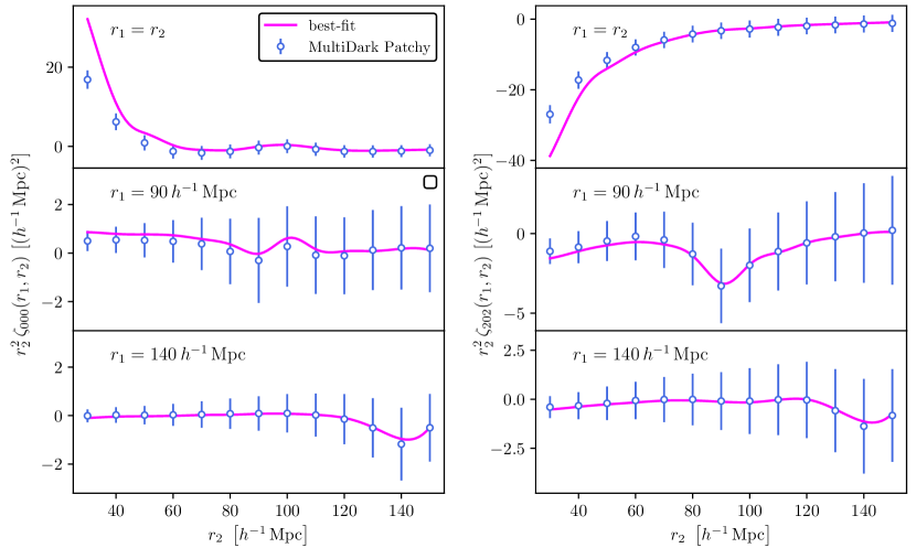
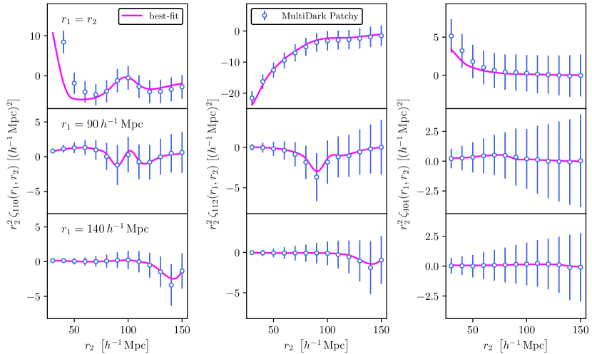
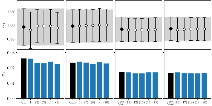
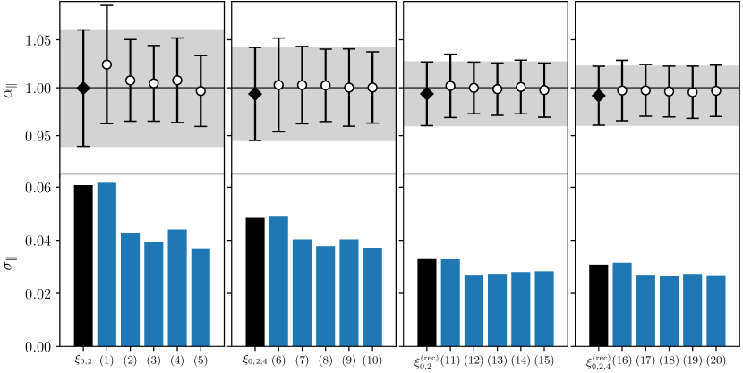
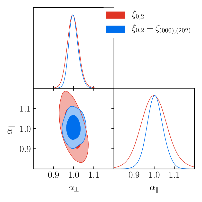
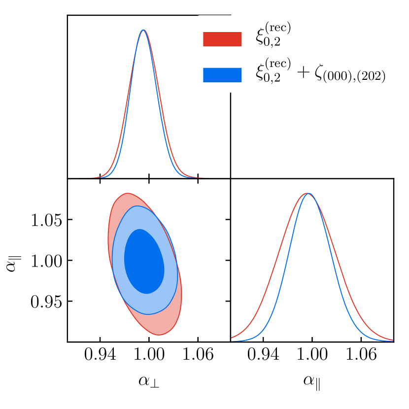
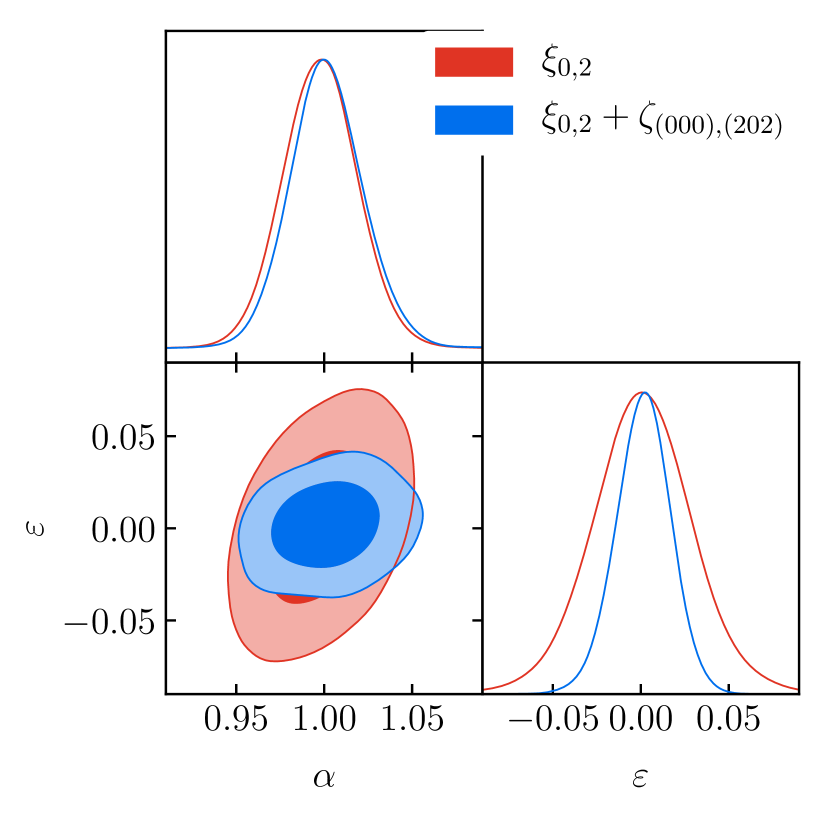
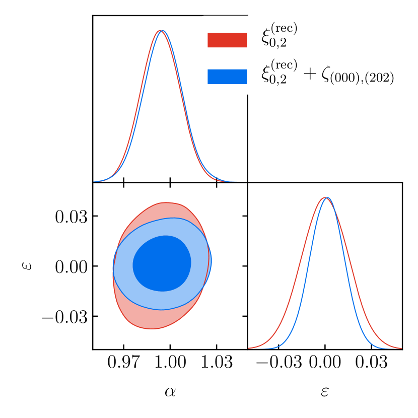
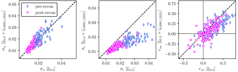
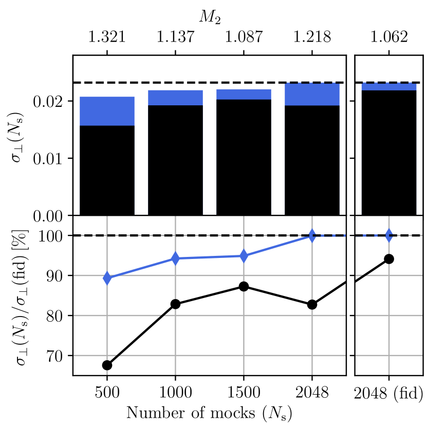
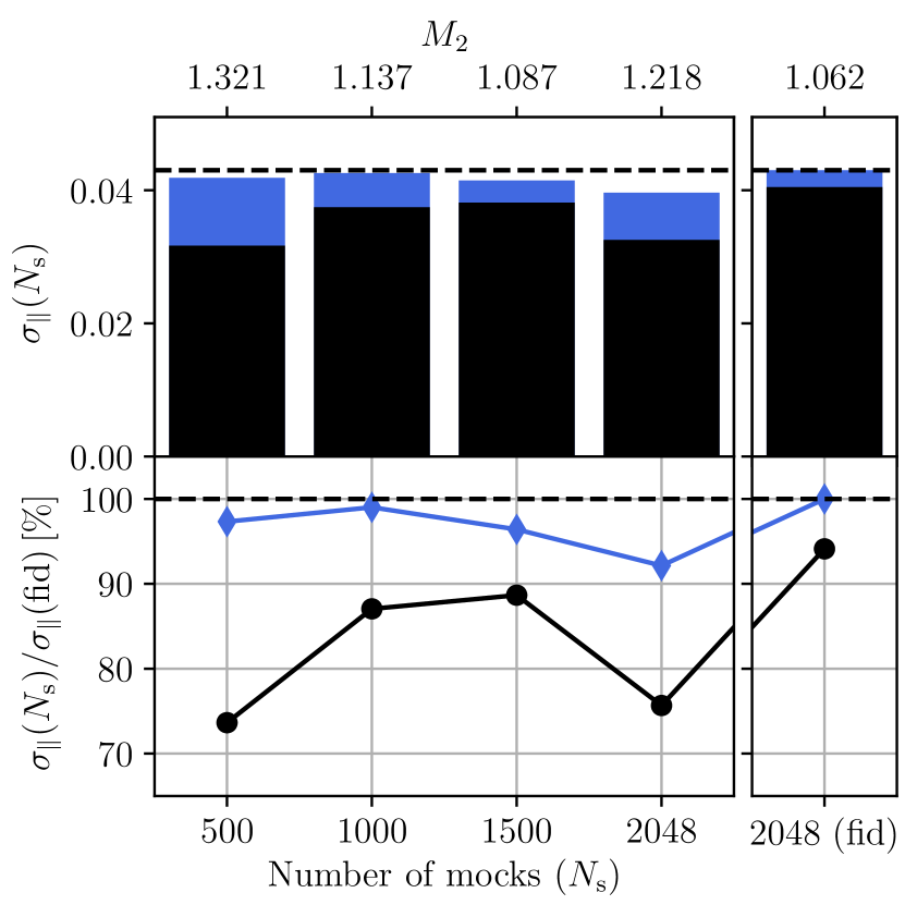
| Patchy mock () | |||||
|---|---|---|---|---|---|
| 0.0021 | 0.022 | 0.0008 | 0.029 | 0.38 | |
| (1) | -0.0028 | 0.023 | 0.0113 | 0.029 | 0.21 |
| (2) | -0.0026 | 0.022 | 0.0033 | 0.018 | 0.18 |
| (3) | -0.0016 | 0.022 | 0.0024 | 0.016 | 0.18 |
| (4) | -0.0025 | 0.023 | 0.0034 | 0.019 | 0.19 |
| (5) | 0.0033 | 0.021 | 0.0006 | 0.016 | 0.12 |
| 0.0031 | 0.023 | -0.0019 | 0.021 | 0.27 | |
| (6) | 0.0001 | 0.022 | 0.0014 | 0.022 | 0.15 |
| (7) | -0.0015 | 0.023 | 0.0014 | 0.017 | 0.17 |
| (8) | -0.0012 | 0.022 | 0.0010 | 0.015 | 0.17 |
| (9) | -0.0011 | 0.023 | 0.0009 | 0.017 | 0.17 |
| (10) | -0.0012 | 0.023 | 0.0005 | 0.015 | 0.13 |
| 0.0062 | 0.014 | -0.0001 | 0.017 | 0.15 | |
| (11) | 0.0044 | 0.015 | 0.0034 | 0.016 | 0.09 |
| (12) | 0.0047 | 0.014 | 0.0026 | 0.013 | 0.11 |
| (13) | 0.0049 | 0.014 | 0.0020 | 0.012 | 0.08 |
| (14) | 0.0044 | 0.014 | 0.0029 | 0.014 | 0.10 |
| (15) | 0.0052 | 0.015 | 0.0017 | 0.013 | 0.10 |
| 0.0064 | 0.013 | -0.0011 | 0.014 | 0.14 | |
| (16) | 0.0055 | 0.014 | 0.0013 | 0.014 | 0.09 |
| (17) | 0.0049 | 0.014 | 0.0013 | 0.012 | 0.09 |
| (18) | 0.0050 | 0.014 | 0.0007 | 0.012 | 0.08 |
| (19) | 0.0053 | 0.014 | 0.0006 | 0.013 | 0.10 |
| (20) | 0.0048 | 0.015 | 0.0001 | 0.012 | 0.06 |
| Patchy mock () | |||||
|---|---|---|---|---|---|
| -0.0008 | 0.0210.0051 | 0.0042 | 0.0280.0075 | 0.320.22 | |
| -0.0060 | 0.0210.0060 | 0.0051 | 0.0180.0036 | 0.170.19 | |
| 0.0008 | 0.0210.0054 | 0.0002 | 0.0210.0052 | 0.260.20 | |
| -0.0047 | 0.0210.0058 | 0.0023 | 0.0160.0031 | 0.140.18 | |
| 0.0033 | 0.0130.0025 | 0.0011 | 0.0160.0037 | 0.140.19 | |
| 0.0023 | 0.0140.0035 | 0.0023 | 0.0130.0024 | 0.070.19 | |
| 0.0038 | 0.0130.0023 | -0.0010 | 0.0140.0024 | 0.120.16 | |
| 0.0028 | 0.0130.0034 | 0.0004 | 0.0120.0020 | 0.040.17 | |
| Patchy mock () | ||||||||
|---|---|---|---|---|---|---|---|---|
| 0.470.085 | – | 1.210.15 | 1.190.24 | – | – | – | – | |
| (1) | 0.520.100 | 0.980.57 | 1.030.19 | 0.910.24 | 0.242.06 | 0.074.10 | -0.170.64 | 0.531.10 |
| (2) | 0.470.089 | 0.880.54 | 1.130.16 | 1.020.25 | 0.391.73 | 0.642.85 | -0.240.67 | 0.381.05 |
| (3) | 0.470.087 | 0.850.52 | 1.130.16 | 1.030.25 | 0.481.62 | 0.552.55 | -0.210.65 | 0.371.01 |
| (4) | 0.470.088 | 0.890.54 | 1.130.16 | 1.030.25 | 0.351.72 | 0.632.89 | -0.250.67 | 0.341.02 |
| (5) | 0.470.089 | 1.000.61 | 1.060.15 | 0.960.23 | 0.341.72 | 0.482.70 | -0.220.71 | 0.401.10 |
| 0.460.082 | – | 1.220.15 | 1.200.23 | – | – | – | – | |
| (6) | 0.500.095 | 0.800.50 | 1.060.17 | 0.960.24 | 0.292.02 | 0.472.65 | -0.080.60 | 0.370.88 |
| (7) | 0.470.086 | 0.880.53 | 1.130.16 | 1.020.25 | 0.331.73 | 0.442.77 | -0.250.67 | 0.361.04 |
| (8) | 0.460.082 | 0.890.55 | 1.140.16 | 1.030.25 | 0.301.72 | 0.572.80 | -0.260.67 | 0.381.04 |
| (9) | 0.460.084 | 0.880.54 | 1.130.16 | 1.020.25 | 0.301.72 | 0.572.80 | -0.260.67 | 0.381.04 |
| (10) | 0.460.082 | 0.850.53 | 1.140.16 | 1.040.25 | 0.371.60 | 0.562.60 | -0.250.64 | 0.341.00 |
| 0.460.075 | – | 1.260.13 | 1.240.20 | – | – | – | – | |
| (11) | 0.490.085 | 0.620.37 | 1.140.14 | 1.030.23 | 0.091.54 | 0.023.27 | -0.140.48 | 0.350.82 |
| (12) | 0.450.078 | 0.680.43 | 1.210.13 | 1.120.22 | 0.391.57 | 0.712.50 | -0.230.58 | 0.250.89 |
| (13) | 0.450.077 | 0.660.41 | 1.210.13 | 1.110.20 | 0.471.46 | 0.662.42 | -0.200.56 | 0.270.84 |
| (14) | 0.450.079 | 0.740.47 | 1.210.13 | 1.070.24 | 0.201.64 | 0.212.50 | -0.320.68 | 0.451.12 |
| (15) | 0.450.076 | 0.770.48 | 1.200.13 | 1.150.21 | 0.161.59 | -0.102.90 | -0.330.63 | -0.070.74 |
| 0.460.075 | – | 1.260.13 | 1.250.20 | – | – | – | – | |
| (16) | 0.480.079 | 0.510.31 | 1.170.14 | 1.090.21 | 0.851.40 | 0.812.12 | 0.010.48 | 0.350.63 |
| (17) | 0.460.077 | 0.660.41 | 1.210.13 | 1.110.22 | 0.371.58 | 0.732.40 | -0.210.57 | 0.310.87 |
| (18) | 0.450.077 | 0.660.41 | 1.200.13 | 1.120.22 | 0.431.42 | 0.542.30 | -0.210.56 | 0.240.83 |
| (19) | 0.450.078 | 0.790.50 | 1.210.13 | 1.110.22 | -0.051.80 | 0.302.43 | -0.380.67 | 0.080.92 |
| (20) | 0.450.076 | 0.680.42 | 1.210.13 | 1.120.23 | 0.371.52 | 0.822.30 | -0.230.58 | 0.260.84 |
| Patchy mock () | ||||||||
|---|---|---|---|---|---|---|---|---|
| 0.460.085 | – | 1.250.15 | 1.220.23 | – | – | – | – | |
| 0.460.089 | 0.960.55 | 1.150.16 | 1.040.23 | 0.291.77 | 0.293.01 | -0.260.69 | 0.361.09 | |
| 0.450.082 | – | 1.250.15 | 1.220.23 | – | – | – | – | |
| 0.460.086 | 0.940.54 | 1.160.15 | 1.040.22 | 0.291.76 | 0.242.97 | -0.250.68 | 0.341.08 | |
| 0.450.077 | – | 1.280.13 | 1.250.20 | – | – | – | – | |
| 0.450.079 | 0.740.43 | 1.220.13 | 1.120.21 | 0.321.58 | 0.382.70 | -0.240.59 | 0.250.92 | |
| 0.450.075 | – | 1.280.13 | 1.260.20 | – | – | – | – | |
| 0.450.077 | 0.720.42 | 1.220.13 | 1.120.21 | 0.321.58 | 0.392.67 | -0.250.58 | 0.250.90 | |