Neural Gaussian Mirror
for Controlled Feature Selection in Neural Networks

Abstract

Deep neural networks (DNNs) have become increasingly popular and achieved outstanding performance in predictive tasks. However, the DNN framework itself cannot inform the user which features are more or less relevant for making the prediction, which limits its applicability in many scientific fields. We introduce neural Gaussian mirrors (NGMs), in which mirrored features are created, via a structured perturbation based on a kernel-based conditional dependence measure, to help evaluate feature importance. We design two modifications of the DNN architecture for incorporating mirrored features and providing mirror statistics to measure feature importance. As shown in simulated and real data examples, the proposed method controls the feature selection error rate at a predefined level and maintains a high selection power even with the presence of highly correlated features.

1 Introduction

Recent advances in deep neural networks (DNNs) significantly improve the state-of-the-art prediction methods in many fields such as image processing, healthcare, genomics, and finance. However, complex structures of DNNs often lead to their lacks of interpretability. In many fields of science, model interpretation is essential for understand the underlying scientific mechanisms and for rational decision-making. At the very least, it is important to know which features are more relevant to the prediction outcome and which are not, i.e., conducting feature selection. Without properly assessing and controlling the reliability of such feature selection efforts, the reproducibility and generalizability of the discoveries are likely unstable. For example, in genomics, current developments lead to good predictions of complex traits using millions of genetic and phenotypic predictors. If one trait is predicted as “abnormal,” it is important for the doctor to know which predictors are active in such a prediction, whether they make medical and biological sense, and whether there exist targeted treatment strategies.

In the classical statistical inference, some $p$-value based methods such as the Benjamini-Hochberg [5] and Benjamini-Yekutieli [6] procedures have been widely employed for controlling the false discovery rate (FDR). However, in nonlinear and complex models, it is often difficult to obtain valid p-values since the analytical form of the distribution of a relevant test statistics is largely unknown. Approximating p-values by bootstrapping and other resampling methods is a valid strategy, but is also often infeasible due to model non-identifiability, (i.e., the existence of multiple equivalent models, such as a DNN with permuted input or internal nodes), complex data and model structures, and high computational costs. In an effect to code with these difficulties, [2] proposed the knockoff filter, which constructs a “fake” copy of the feature matrix that is independent of the response but retains the covariance structure of the original feature matrix (also called the “design matrix”). Important features can be selected after comparing inferential results for the true features with those for the knockoffs. To extend the idea to higher dimensional and more complex models, [9] further proposed the Model-X knockoff, which considers a random design with known joint distribution (Gaussian) of the input features. Recently, [34] develops the PCS inference to investigate the stability of the data by introducing perturbations to the data, the model, and the algorithm. Dropout [29] and Gaussian Dropout can be viewed as examples of model perturbations, which are efficient for reducing the instability and elevating out-of-sample performances.

For enhancing interpretability, feature selection in neural networks has attracted some recent attention. To this end, gradients with respect to each input are usually taken as an effective measurement of feature importance in convolutional and multi-layer neural networks as shown in [18]. [27] selects features in DNNs based on changes of the cross-validation (CV) classification error rate caused by the removal of an individual feature. However, how to control the error of such a feature selection process in DNNs is unclear. A recent work by [22] utilizes the Model-X Knockoff method to construct a pairwisely-connected input layer to replace the original one, and the latent “competition” within each pair separates important features from unimportant ones by the measurement of knockoff statistics. However, the Model-X method requires that the distribution of $\bm{X}$ be either known exactly, or known to be in a nice distribution family that possesses simple sufficient statistics [20]. Also, the construction procedure for the knockoffs in [22] is based on the Gaussian assumption on the input features, which is not satisfied in many applications such as genome wide association studies with discrete input data. In addition, the DeepPINK does not fit exactly the purpose of network interpretation since the input layer is not fully connected to hidden layers, and thus some of the connections in the “original” structure may be lost in this specific Pairwise-Input structure.

In this paper, we introduce the neural Gaussian mirror (NGM) strategy for feature selection with controlled false selection error rates. NGM does not require any knowledge about or assumption on the joint distribution of the input features. Each NGM is created by perturbing an input feature explicitly. For example, for the $j$th feature, we create two mirrored features as $\bm{X}_{j}^{+}=\bm{X}_{j}+c_{j}\bm{Z}_{j}$ and $\bm{X}_{j}^{-}=\bm{X}_{j}-c_{j}\bm{Z}_{j}$, where $\bm{Z}_{j}$ is the vector of i.i.d. standard Gaussian random variables. The scalar $c_{j}$ is chosen so as to minimize the dependence between $\bm{X}_{j}^{+}$ and $\bm{X}_{j}^{-}$ conditional on the remaining variables, $\bm{X}_{-j}$. To cope with nonlinear dependence, we introduce a kernel-based conditional independence measure and obtain $c_{j}$ by solving an optimization problem. Then, we construct two modifications of the network architectures based on the mirrored design. The proposed mirror statistics tend to take large positive values for important features and are symmetric around zero for null features, which enables us to control the selection error rate.

2 Background

2.1 Controlled feature selection

In many modern applications, we are not only interested in fitting a model (with potentially many predictors) that can achieve a high prediction accuracy, but also keen in selecting relevant features with controlled false selection error rate. Mathematically, we consider a general model with an unknown link function $F$ illustrating the connection between the response variable $Y$ and $p$ predictor variables $X\in\mathbb{R}^{p}$: $Y=F(X)+\epsilon$, where $\epsilon$ denotes the random noise.

We define $S_{0}$ to be the set of “null” features: $\forall\ k\in S_{0}$, we have $Y\perp\!\!\!\!\perp X_{j}\mid X_{-j}$, where $X_{-j}=\{X_{1},\dots,X_{p}\}\backslash\{X_{j}\}$ and define $S_{1}=\{1,\dots,p\}\backslash S_{0}$ as the set for relevant features. Feature selection is equivalent to recovering $S_{1}$ based on observations. When the estimated set $\widehat{S}_{1}$ is produced, the false discoveries can be denoted as $\widehat{S}_{1}\cap S_{1}^{c}$, where $S_{1}$ is the true set of important features. The false discovery proportion (FDP) is defined as

$$\text{FDP}=\frac{|\widehat{S}_{1}\cap S_{1}^{c}|}{|\widehat{S}_{1}|},$$ (2.1)

and its expectation is called the false discovery rate (FDR), i.e., ${\rm FDR}=\mathbb{E}[{\rm FDP}]$.

Technically, controlled feature selection methods are different from conventional feature selection methods such as Lasso in that the former require additional efforts in assessing the selection uncertainty by means of estimating the FDP, which becomes more challenging in DNNs.

2.2 Gaussian mirror design for linear models

To discern relevant features from irrelevant ones, we intentionally perturb the input features via the following Gaussian mirror design: for each feature $X_{j}$, we construct a mirrored pair $(X_{j}^{+},X_{j}^{-})=(X_{j}+c_{j}Z_{j},X_{j}-c_{j}Z_{j})$ with $Z_{j}\sim N(0,1)$ being independent of all the $X$. We call $(X_{j}^{+},X_{j}^{-},X_{-j})$ the $j$-th mirror design. Regressing $Y$ on the $j$-th mirror design, we obtain coefficients via the ordinary least squares (OLS) method. Let $\widehat{\beta}_{j}^{+}$ and $\widehat{\beta}_{j}^{-}$ be the estimated coefficients for $X_{j}^{+}$ and $X_{j}^{-}$, respectively. The mirror statistics for the $j$th feature is defined as:

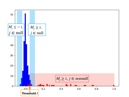
Figure 1: Histogram of mirror statistics: red represents important variables and blue stands for null variables

$$M_{j} =|\widehat{\beta}_{j}^{+}+\widehat{\beta}_{j}^{-}|-|\widehat{\beta}_{j}^{+}-\widehat{\beta}_{j}^{-}|$$ (2.2)

For important features $j\in S_{1}$, $\widehat{\beta}_{j}^{+}$ tends to be similar to $\widehat{\beta}_{j}^{-}$, which helps cancel out the perturbation part leading to a large positive value of $M_{j}$. From another point of view, the large value of $M_{j}$ indicates that the importance of the $j$th features is more stable to the perturbation, i.e. $\widehat{\beta}_{j}^{+}\approx\widehat{\beta}_{j}^{-}$. For null features $j\in S_{0}$, the mirror statistics can be made symmetric about zero by choosing a proper $c_{j}$ as detailed in Theorem 2.1.

Theorem 2.1

Assume $Y=X\beta+\epsilon$ where $\epsilon$ is Gaussian white noise. Let $X_{j}^{+}=X_{j}+cZ_{j}$, $X_{j}^{-}=X_{j}-cZ_{j}$, and $I^{L}_{j}(c)=\rho_{X_{j}^{+}X_{j}^{-}\cdot X_{-j}}$, i.e., the partial correlation of $X_{j}^{+}$ and $X_{j}^{-}$ given $X_{-j}$. For any $j\in S_{0}$, if we set

$$c_{j}=\arg\min_{c}[I^{L}_{j}(c)]^{2},$$ (2.3)

then we have $P(M_{j}<-t)=P(M_{j}>t)$ for any $t>0$.

A detailed proof of the theorem can be found in [31]. It shows that the symmetric property of the mirror statistics $M_{j}$ for null features is satisfied if we choose $c_{j}$ that minimizes the magnitude of the partial correlation $I^{L}_{j}(c)$, which is equivalent to solving $I^{L}_{j}(c)=0$ in linear models. In other words, the perturbation $c_{j}Z_{j}$ makes $X_{j}^{+}$ and $X_{j}^{-}$ partially uncorrelated given $X_{-j}$.

We note that in linear models with OLS fitting, the above construct is equivalent to generating an independent noise feature $c_{j}Z$ and regress $Y$ on $(\bm{X},c_{j}Z)$. The mirror statistic is simply the magnitude difference between the estimated coefficient for $X_{j}$ and that for $c_{j}Z$. However, this simpler construct is no longer equivalent to the original design for nonlinear models or for high-dimensional linear models where the OLS is not used for fitting. Also, the conditional independence motivation for choosing $c_{j}$ is lost in this simpler formulation.

Figure 1 shows the distribution of the $M_{j}$’s. It is seen that relevant features can be separated from the null ones fairly well and a consistent estimate of the false discoveries proportion based on the symmetric property can be obtained.

For a threshold $t$, we select features as $\widehat{S}_{1}=\{j:M_{j}\geq t\}$. The symmetric property of $M_{j}$ for $j\in S_{0}$ implies that $\mathbb{E}[\#\{j\in S_{0}:\;M_{j}\geq t\}]=\mathbb{E}[\#\{j\in S_{0}:\;M_{j}\leq-t\}]$. Thus we obtain an estimate of the FDP as

$$\widehat{FDP}(t)=\frac{\#\{j:M_{j}\leq-t\}}{\#\{j:M_{j}\geq t\}\vee 1}$$ (2.4)

In practice, we choose a data adaptive threshold

$$\tau_{q}=\min_{t}\{t>0:\widehat{FDP}(t)\leq q\}$$ (2.5)

to control the FDR at a predefined level $q$.

As shown in Theorem 4 of [31], under weak dependence assumption of $M_{j}$s, we have

$$\mathbb{E}[FDP(\tau_{q})]<q$$

as $p$ goes to infinity, i.e., the FDR is asymptotically controlled under the predefined threshold $q$.

3 Neural Gaussian mirror

We here describe a model-free mirror design for controlling variable selection errors in DNNs. In linear models, a key step of our mirror design is to choose a proper perturbation level $c_{j}$ so as to annihilate the partial correlation between the mirror variables $X_{j}^{+}$ and $X_{j}^{-}$. Since the partial correlation being zero for two random variables implies that they are conditional independence under the joint Gaussian assumption, for more complex models such as DNNs, we consider a general kernel-based measure of conditional dependence between $X_{j}^{+}$ and $X_{j}^{-}$ and choose $c_{j}$ by minimizing this measure. Then, we can construct the mirror statistics and establish a data-adaptive threshold to control the selection error rate in a similar way as in linear models. We call this whole procedure the neural Gaussian mirror (NGM).

3.1 Model-free mirror design

Without any specific model assumption, we construct the mirrored pair as

$$(\bm{X}_{j}^{+},\bm{X}_{j}^{-})=(\bm{X}_{j}+c_{j}\bm{Z}_{j},\bm{X}_{j}-c_{j}\bm{Z}_{j}),$$

where $\bm{Z}_{j}\sim N(0,I_{n})$, and $c_{j}$ is chosen as

$$c_{j} ={\rm arg}\min_{c}[I^{K}_{j}(c)]^{2}$$ (3.1)

Here $[I_{j}^{K}(c)]^{2}$ is a kernel-based conditional independence measure between $X_{j}^{+}$ and $X_{j}^{-}$ given $X_{-j}$. We give a detailed expression of $[I_{j}^{K}(c)]^{2}$ in Sections 3.2 and 3.3. Compared with (2.3), the kernel-based mirror design can incorporate nonlinear dependence effectively.

3.2 Decomposition of log-density function

For notational simplicity, we write $(U,V,W)=(X_{j}+cZ,X_{j}-cZ,X_{-j})$ and denote their log-transferred joint density function as $\eta$, which belongs to a tensor product reproducing kernel Hilbert space (RKHS) $\mathcal{H}$ [21]. We define $\mathcal{H}=\mathcal{H}^{U}\otimes\mathcal{H}^{V}\otimes\mathcal{H}^{W}$, where $\mathcal{H}^{U}$, $\mathcal{H}^{V}$ and $\mathcal{H}^{W}$ are marginal RKHSs and “$\otimes$” denotes the tensor product of two vector spaces. We decompose $\eta$ as

$$\eta(u,v,w)=\eta_{U}(u)+\eta_{V}(v)+\eta_{W}(w)+\eta_{U,W}(u,w)\\ +\eta_{V,W}(v,w)+\eta_{U,V}(u,v)+\eta_{U,V,W}(u,v,w).$$ (3.2)

The uniqueness of the decomposition is guaranteed by the probabilistic decomposition of $\mathcal{H}$.

For simplicity, we use the Euclidean space as an example to illustrate the basic idea of tensor sum decomposition, which is also known as ANOVA decomposition in linear models. For example, for the $d$-dimensional Euclidean space, we let $f$ be a vector and let $f(x)$ be its $x$-th entry, $x=1,\dots,d$. Suppose $\mathcal{A}$ is the average operator defined as $\mathcal{A}f(x)=\left\langle\delta,f\right\rangle$, where $\delta=(\delta_{1},\dots,\delta_{d})$ is a probability vector (i.e., $\delta_{i}\geq 0$, and $\sum\delta_{i}=1$). The tensor sum decomposition of the Euclidean space $\mathbb{R}^{d}$ is

$$\mathbb{R}^{d}=\mathbb{R}^{d}_{0}\oplus\mathbb{R}^{d}_{1}:=\{\delta\}\oplus\{f\in\mathbb{R}^{d}\,|\,\sum_{x=1}^{d}\delta_{x}f(x)=0\},$$

where the first space is called the grand mean and the second space is called the main effect. Then, we construct the kernel for $\mathbb{R}^{d}_{0}$ and $\mathbb{R}^{d}_{1}$ as in Lemma A.2 in the Supplementary Material (SM).

However, in RKHS of infinite dimension, the grand mean is not a single vector. Here, we set the average operator $\mathcal{A}_{l}$ as $\mathcal{A}_{l}:=f\to E_{x}f(x)=E_{x}\left\langle K^{l}_{x},f\right\rangle_{\mathcal{H}^{l}}=\left\langle E_{x}K^{l}_{x},f\right\rangle_{\mathcal{H}^{l}}$ where $K^{l}$ is the kernel function in $\mathcal{H}^{l}$ and the first equality is due to the reproducing property. $E_{x}K^{l}_{x}$ plays the same role as $\delta$ in Euclidean space. Then we have the tensor sum decomposition of marginal RKHS $\mathcal{H}^{l}$ defined as

$$\mathcal{H}^{l}=\mathcal{H}^{l}_{0}\oplus\mathcal{H}^{l}_{1}:=\{E_{x}K_{x}\}\oplus\{f\in\mathcal{H}^{l}:\mathcal{A}_{l}f=0\}.$$ (3.3)

Following the same fashion, we call $\mathcal{H}^{l}_{0}$ as the grand mean space and $\mathcal{H}^{l}_{1}$ as the main effect space. Note that $E_{x}K^{l}_{x}$ is also known as the kernel mean embedding, which is well established in the statistics literature [7]. We show the kernel functions for $\mathcal{H}^{l}_{0}$ and $\mathcal{H}^{l}_{1}$ in Lemma A.3 (see SM for details).

Following [17], we apply the distributive law and have the decomposition of $\mathcal{H}$ as

$$\mathcal{H}= (\mathcal{H}^{U}_{0}\oplus\mathcal{H}^{U}_{1})\otimes(\mathcal{H}^{V}_{0}\oplus\mathcal{H}^{V}_{1})\otimes(\mathcal{H}^{W}_{0}\oplus\mathcal{H}^{W}_{1})$$

$$\equiv \mathcal{H}_{000}\oplus\mathcal{H}_{100}\oplus\mathcal{H}_{010}\oplus\mathcal{H}_{001}\oplus\mathcal{H}_{110}\oplus\mathcal{H}_{101}$$

$$\oplus\mathcal{H}_{011}\oplus\mathcal{H}_{111}$$ (3.4)

where $\mathcal{H}_{ijk}=\mathcal{H}^{U}_{i}\otimes\mathcal{H}^{V}_{j}\otimes\mathcal{H}^{W}_{k}$. We show the kernel functions for each subspace in Lemma A.4 (see SM). Each component in (3.2) is the projection of $\eta$ on the corresponding subspace in (3.4). Thus, the decomposition of the log-density function in (3.2) is unique.

We introduce the following lemma to establish a sufficient and necessary condition for the conditional independence of $U$ and $V$ given $W$ based on the decomposition in (3.2).

Lemma 3.1

Assume that the log-joint-density function $\eta$ of $(U,V,W)$ belongs to a tensor product RKHS. $U$ and $V$ are conditional independent if and only if $\eta_{U,V}+\eta_{U,V,W}=0$.

Here $\eta_{\mathcal{C}}$ is the function only of variables in the set $\mathcal{C}$. The proof of this lemma is given in SM. Lemma 3.1 implies that the following two hypothesis testing problems are equivalent:

$$H_{0}:U\perp\!\!\!\!\perp V\mid W\mbox{ vs. }H_{1}:U\not\!\perp\!\!\!\perp V\mid W$$ (3.5)

and

$$H_{0}:\eta\in\mathcal{H}_{0}\mbox{ vs. }H_{1}:\eta\in\mathcal{H}/\mathcal{H}_{0},$$ (3.6)

where $\mathcal{H}_{0}:=\mathcal{H}_{000}\oplus\mathcal{H}_{100}\oplus\mathcal{H}_{010}\oplus\mathcal{H}_{001}\oplus\mathcal{H}_{011}\oplus\mathcal{H}_{101}$. Compared to (3.5), a key advantage of (3.6) is that we are able to specify the function space of the log-transferred density under both null and alternative.

3.3 Kernel-based Conditional Dependence Measure

Let $\bm{t}_{i}=(U_{i},V_{i},W_{i})$, $i=1,\ldots,n$, be i.i.d. observations generated from the distribution of ${\mathcal{T}}=(U,V,W)$. The log-likelihood-ratio functional is

$$\begin{split}LR_{n}(\eta)&=\ell_{n}(\eta)-\ell_{n}(P_{\mathcal{H}_{0}}\eta)\\ &=-\frac{1}{n}\sum_{i=1}^{n}\{\eta(\bm{t}_{i})-P_{\mathcal{H}_{0}}\eta(\bm{t}_{i})\},\,\,\eta\in\mathcal{H},\end{split}$$ (3.7)

where $P_{\mathcal{H}_{0}}$ is a projection operator from $\mathcal{H}$ to $\mathcal{H}_{0}$. Using the reproducing property, we rewrite (3.7) as

$$LR_{n}(\eta)=-\frac{1}{n}\sum_{i=1}^{n}\left\{\left\langle K^{\mathcal{H}}_{\bm{t}_{i}},\eta\right\rangle_{\mathcal{H}}-\left\langle K^{\mathcal{H}_{0}}_{\bm{t}_{i}},\eta\right\rangle_{\mathcal{H}}\right\},$$ (3.8)

where $K^{\mathcal{H}}$ is the kernel for $\mathcal{H}$ and $K^{\mathcal{H}_{0}}$ is the kernel for $\mathcal{H}_{0}$. Then, we calculate the Fréchet derivative of the likelihood ratio functional as

$$DLR_{n}(\eta)\Delta\eta =\left\langle\frac{1}{n}\sum_{i=1}^{n}(K^{\mathcal{H}}_{\bm{t}_{i}}-K^{\mathcal{H}_{0}}_{\bm{t}_{i}}),\Delta\eta\right\rangle_{\mathcal{H}}$$

$$=\left\langle\frac{1}{n}K^{1}_{\bm{t}_{i}},\Delta\eta\right\rangle_{\mathcal{H}}$$ (3.9)

where $K^{1}$ is the kernel for $\mathcal{H}_{110}\oplus\mathcal{H}_{111}$. The score function $\frac{1}{n}K_{\bm{t}_{i}}^{1}$ is the first order approximation of the likelihood ratio functional. We define our kernel-based conditional measure as the squared norm of the score function of the likelihood ratio functional as

$$[I_{j}^{K}(c)]^{2}=\left\|\frac{1}{n}\sum_{i=1}^{n}K^{1}_{\bm{t}_{i}}\right\|_{\mathcal{H}}^{2},$$ (3.10)

which, by the reproducing property, can be expanded as

$$[I_{j}^{K}(c)]^{2}=\frac{1}{n^{2}}\sum_{i=1}^{n}\sum_{j=1}^{n}K^{1}(\bm{t}_{i},\bm{t}_{j}).$$ (3.11)

The construction of $[I_{j}^{K}(c)]^{2}$ is related to the kernel conditional independence test [13], which generalizes the conditional covariance matrix to a conditional covariance operator in RKHS. However, the calculation of the norm of the conditional covariance operator involves the inverse of an $n\times n$ matrix, which is expensive to obtain when the sample size $n$ is large. But we will show that our proposed score test statistics only involve matrix multiplications.

We introduce a matrix form of the squared norm of score function to facilitate the computation process. In (3.11), $[I_{j}^{N}(c)]^{2}$ is determined by the kernel on $\mathcal{H}^{U}_{1}\otimes\mathcal{H}^{V}_{1}\otimes\mathcal{H}^{W}_{0}\oplus\mathcal{H}^{U}_{1}\otimes\mathcal{H}^{V}_{1}\otimes\mathcal{H}^{W}_{1}$. Thus, by Lemma A.2 and Lemma A.3, we can rewrite (3.11) as

$$[I_{j}^{K}(c)]^{2}=\frac{1}{n^{2}}[(HK^{U}H)\circ(HK^{V}H)\circ K^{W}]_{++}$$ (3.12)

where $H=I_{n}-\frac{1}{n}\mathbf{1}\mathbf{1}^{T}$, $I_{n}$ is a $n\times n$ identity matrix and $\mathbf{1}_{n}$ is a $n\times 1$ vector of ones, and $[A]_{++}=\sum_{i=1}^{n}\sum_{j=1}^{n}A_{ij}$.The most popular kernel choices are Gaussian and polynomial kernels. With parallel computing, the computational complexity for using either is approximately linear in $n$.

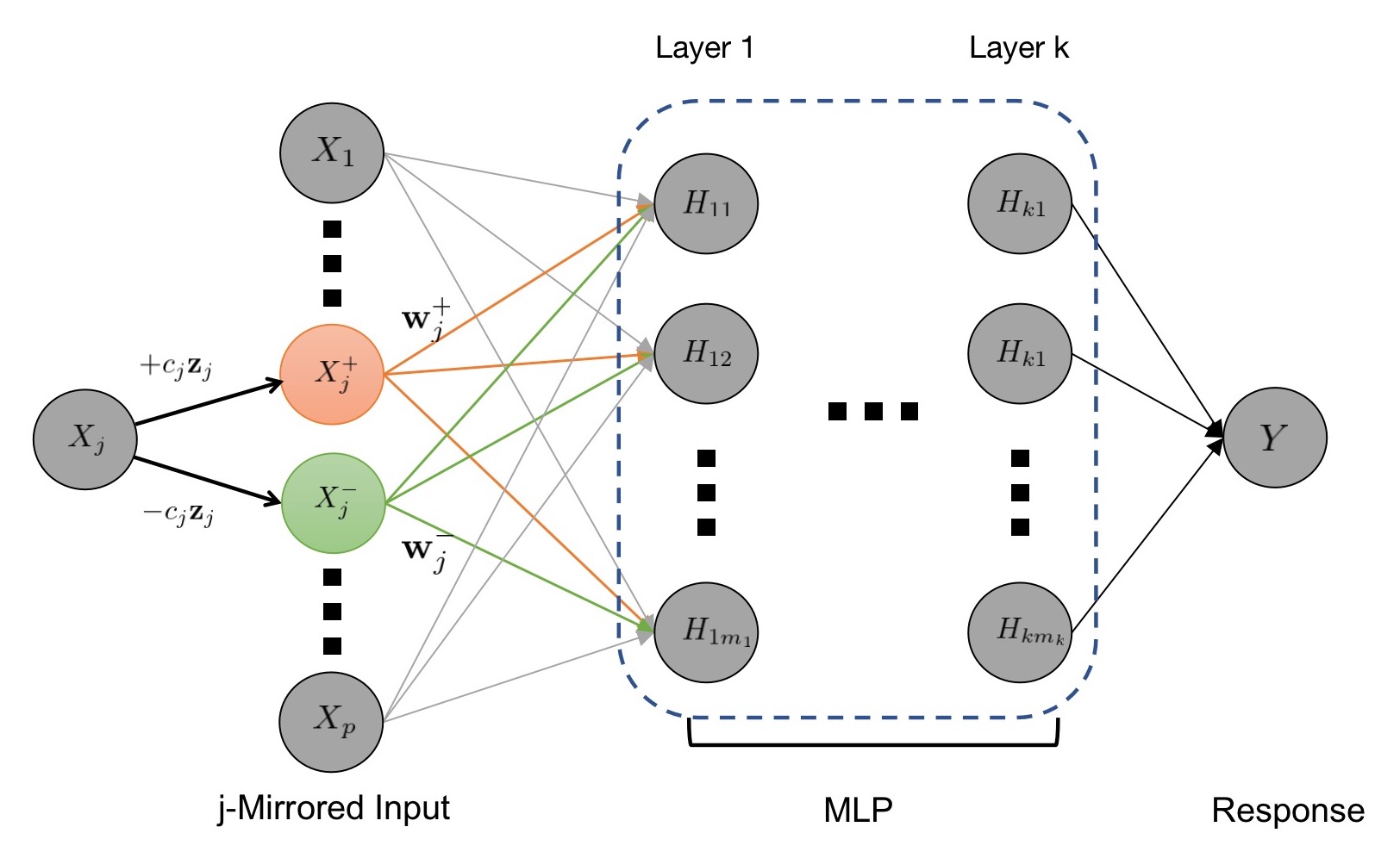
Figure 2: Indivdual neural Gaussian mirror in DNN

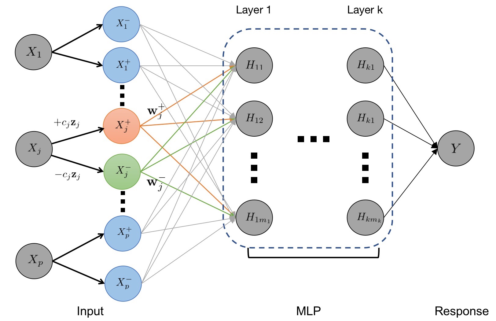
Figure 3: Simultaneous neural Gaussian mirror in DNN

3.4 Mirror Statistics in DNNs

In order to construct mirror statistics in DNNs, we introduce an importance measure for each input feature as a generalization of the connection weights method proposed by [10]. We consider a fully connected multi-layer perceptron (MLP) with $k$ hidden layers denoted as $(H^{(t)}_{1},\dots,H^{(t)}_{n_{t}})$ for $t=1,\dots,k$. The connection between the $t$-th and $(t+1)$-th layers can be expressed as

$$H_{j}^{(t+1)}=g_{t+1}(\sum_{i=1}^{n_{t}}w_{ij}^{(t)}H_{i}^{(t)}),\ \mbox{for }\ j=1,\dots,n_{t+1},$$

where $g_{t+1}$ is the activation function. We let $t=0$ and $t=k+1$ denote the input and output layers, respectively.

For a path $\bm{l}=(X_{j},H_{i_{1}}^{(1)},...,H_{i_{k}}^{(k)},y)$ through the network, We define its accumulated weight as

$$\delta(\bm{l})=\omega_{ji_{1}}^{(0)}\omega^{(k)}_{i_{k}1}\prod_{t=1}^{k-1}\omega^{(t)}_{i_{t}i_{t+1}}.$$

Let $\bm{\Omega}^{(0)}_{j}=(\omega_{j1}^{(0)},\dots,\omega_{jn_{1}}^{(0)})$ be the weight vector connecting $X_{j}$ with the first layer. We define the feature importance of $X_{j}$ as

$$L(X_{j})=\sum_{\bm{l}\in P_{j}}\delta(\bm{l})=\langle\bm{C},\bm{\Omega}^{(0)}_{j}\rangle,$$ (3.13)

where $P_{j}$ is the set consisting of all paths connecting $X_{j}$ to $y$ with one node in each layer and $\bm{C}=\prod_{t=1}^{k}\bm{\Omega}^{(t)}$, where $\bm{\Omega}^{(t)}_{ij}=\omega_{ij}^{(t)}\in\mathbb{R}^{n_{t}\times n_{t+1}}$ for $i=1,\dots,n_{t}$ and $j=1,\dots,n_{t+1}$. The gradient w.r.t. each input feature $\partial y/\partial X_{j}$ in [18] is a modified version of $L(X_{j})$ (see the SM for details).

Based on (3.13), we define mirror statistics as

$$M_{j}=|L(X_{j}^{+})+L(X_{j}^{-})|-|L(X_{j}^{+})-L(X_{j}^{-})|,$$ (3.14)

and use (2.4) to estimate FDP. By setting a predefined error rate $q$, a data adaptive threshold is given by $\tau_{q}=\min_{t}\{t>0:\widehat{FDP}(t)\leq q\}$ and $\widehat{S}_{1}=\{j:M_{j}\geq\tau_{q}\}$ is the set of selected features.

4 Implementations

4.1 Two forms of neural Gaussian mirror

The NGM can be realized in two ways: individual or simultaneous. As shown in Figure 2, the individual neural Gaussian mirror (INGM) is constructed by treating one feature a time. More specifically, for feature $\bm{X}_{j}$, we create $\bm{X}_{j}^{+}$ and $\bm{X}_{j}^{-}$ with $c_{j}$ minimizing $[I_{j}^{K}(c)]^{2}$. Then, we set the input layer as $(X_{1},\dots,X_{j}^{+},X_{j}^{-},\dots,X_{p})$ and fit the MLP as shown in Figure 2. For any predefined error rate $q$, we select feature by Algorithm 1.

Algorithm 1 Individual NGM: feature selection in deep neural networks

Input: Fixed FDR level $q$, $(\bm{x}_{i},y_{i})$, $i=1,...,n$ with $\bm{x}_{i}\in\mathbb{R}^{p}$, $y_{i}\in\mathbb{R}^{1}$
Output: $\widehat{S}_{1}$

1:for $i=1$ to $p$ do

2:     Generate $\bm{Z}_{j}\sim\mathcal{N}(0,\bm{I}_{n})$

3:     Compute $c_{j}={\rm arg}\min_{c}[I_{j}^{K}(c)]^{2}$

4:     Create mirrored pair$(\bm{X}_{j}^{+},\bm{X}_{j}^{-})=(\bm{X}_{j}+c_{j}\bm{Z}_{j},\bm{X}_{j}-c_{j}\bm{Z}_{j})$

5:     Train MLP with $\bm{X}^{(j)}=(\bm{X}_{j}^{+},\bm{X}_{j}^{-},\bm{X}_{-j})$ as the input layer

6:     Compute mirror statistics $M_{j}$ by (3.14)

7:end for

8:Calculate $T=\min\{t>0:\widehat{FDP}(t)\leq q\}$.

9:Return $\widehat{S}_{1}\leftarrow\{j:\;M_{j}\geq T\}$.

To increase the efficiency, we construct the simultaneous neural Gaussian mirror (SNGM), by mirroring all the $p$ features at the same time as shown in Figure 3. The input layer include all mirrored pairs, i.e., $(X_{1}^{+},X_{1}^{-},\dots,X_{p}^{+},X_{p}^{-})$. The detailed algorithm is given in Algorithm 2.

Algorithm 2 SNGM: Feature selection with simultaneous-mirrored Pairs

Input: Fixed FDR level $q$, $(\bm{x}_{i},y_{i})$, $i=1,...,n$ with $\bm{x}_{i}\in\mathbb{R}^{p}$, $y_{i}\in\mathbb{R}^{1}$
Output: $\widehat{S}_{1}$

1:for $i=1$ to $p$ do

2:     Generate $\bm{Z}_{j}\sim\mathcal{N}(0,\bm{I}_{n})$

3:     Compute $c_{j}={\rm arg}\min_{c}[I_{j}^{K}(c)]^{2}$

4:     Create mirrored pair $(\bm{X}_{j}^{+},\bm{X}_{j}^{-})=(\bm{X}_{j}+c_{j}\bm{Z}_{j},\bm{X}_{j}-c_{j}\bm{Z}_{j})$

5:end for

6:Train MLP with input layer as $(\bm{X}_{1}^{+},\bm{X}_{1}^{-},\dots,\bm{X}_{p}^{+},\bm{X}_{p}^{-})$.

7:Calculate $M_{j}$ by (3.14) for $j=1,\dots,p$.

8:Calculate $T=\min\{t>0:\widehat{FDP}(t)\leq q\}$.

9:Output $\widehat{S}_{1}\leftarrow\{j:\;M_{j}\geq T\}$.

4.2 Screening

To further reduce the computational cost, we propose a screening step based on the rank of feature importance measure defined in (3.13). The screening procedure is inspired by the RANK method proposed by [11, 22], which uses part of the data for estimating the precision matrix and subset selection and leaves the remaining data for controlled feature selection.

In the screening procedure, we first randomly select $[n/3]$ samples $(\bm{X}^{(1)},\bm{y}^{(1)})$ to train a neural network. We calculate feature importance measure $\{L(\bm{X}^{(1)}_{j})$ for $j=1,2,\dots,p\}$ and rank their absolute values from large to small as $|L|_{(1)}\geq|L|_{(2)}\geq\dots\geq|L|_{(p)}$. We denote $\widehat{S}_{m}=\{j:L(\bm{X}^{(1)}_{j})\geq|L|_{(m)}\}$ as our screened set. Empirically, we can set $m$ as $[n/2]$ or $[2n/log(n)]$. The screening can be implemented before the INGM and the SNGM algorithms to save computational costs. we call the INGM with screening and SNGM with screening as S-INGM and S-SNGM, respectively.

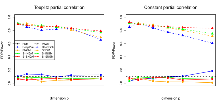
Figure 4: Performance comparison of NGMs and DeepPINK with predefined FDR level $q=0.1$ in linear models with two partial correlation structures

Table 1: Varying single-index link functions with two PC (partial correlation) structures (q=0.1)

Setting	$n=1000$	Link function	S-SNGM		SNGM		S-INGM		DeepPink
			FDR	Power	FDR	Power	FDR	Power	FDR	Power
Toeplitz PC	$p=500$	$f_{1}(t)=t+sin(t)$	0.071	0.867	0.045	0.857	0.057	0.900	0.085	0.900
		$f_{2}(t)=0.5t^{3}$	0.092	0.873	0.080	0.843	0.061	0.830	0.155	0.413
		$f_{3}(t)=0.1t^{5}$	0.059	0.865	0.071	0.847	0.132	0.807	0.148	0.333
	$p=2000$	$f_{1}(t)=t+sin(t)$	0.085	0.843	0.081	0.820	0.084	0.837	0.126	0.817
		$f_{2}(t)=0.5t^{3}$	0.076	0.788	0.082	0.587	0.081	0.810	0.149	0.320
		$f_{3}(t)=0.1t^{5}$	0.093	0.737	0.108	0.530	0.185	0.620	0.477	0.053
Constant PC	$p=500$	$f_{1}(t)=t+sin(t)$	0.057	0.880	0.067	0.877	0.070	0.900	0.136	0.86
		$f_{2}(t)=0.5t^{3}$	0.084	0.870	0.047	0.867	0.057	0.847	0.084	0.587
		$f_{3}(t)=0.1t^{5}$	0.066	0.867	0.066	0.847	0.027	0.802	0.143	0.46
	$p=2000$	$f_{1}(t)=t+sin(t)$	0.055	0.857	0.012	0.833	0.057	0.813	0.094	0.800
		$f_{2}(t)=0.5t^{3}$	0.064	0.787	0.016	0.613	0.104	0.803	0.174	0.313
		$f_{3}(t)=0.1t^{5}$	0.080	0.743	0.020	0.548	0.111	0.607	0.412	0.147

5 Numerical simulations

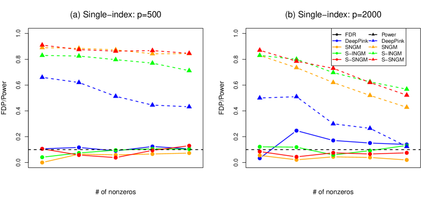
Figure 5: Performance comparison of NGM and DeepPINK with predefined FDR level $q=0.1$ under single-index model with link function $f_{2}$. The triangle dots denote power and round dots denote FDR. (a). p=500; (b). p=2000

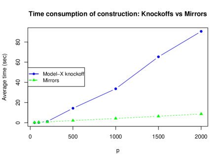
Figure 6: Computational time for constructing input variables: Mirrors vs Model-X Knockoffs

We choose an MLP structure with two hidden layers, with $N_{1}=20log(p)$ and $N_{2}=10log(p)$ hidden nodes respectively.We compare the selection power and FDR of NGMs with the DeepPINK, and conduct experiments in both simulated and real-data settings with $20$ repetitions. In the simulation studies, we consider data from both linear models and nonlinear models. In each setting we consider two covariance structures for $\bm{X}$: the Toeplitz partial correlation structure and the constant partial correlation structure. The Toeplitz partial correlation structure has its precision matrix (i.e., inverse) as $\bm{\Omega}=(\rho^{|i-j|})$. The constant partial correlation structure has its precision matrix as $\bm{\Omega}=(1-\rho)\bm{I}_{p}+\rho\bm{J}_{p}$ where $\bm{J}_{p}=\frac{1}{p}\bm{1}_{p}\bm{1}_{p}^{T}$, where $\rho=0.5$.

5.1 Linear models

First, we examine the performance of all methods in linear models: $y_{i}=\bm{\beta}^{\top}\bm{x}_{i}+\epsilon_{i},\ \epsilon_{i}\stackrel{{\scriptstyle\mbox{\small{i.i.d.}}}}{{\sim}}N(0,1)$, for $i=1,\dots,n$. We randomly set $k=30$ elements in $\bm{\beta}$ to be nonzero and generated from $\mathcal{N}(0,(20\sqrt{log(p)/n})^{2})$ to mimic various signal strengths in real applications.

As shown in Figure 4, NGMs control the FDR at $q=0.1$ and have a higher power than the DeepPINK. In the constant partial correlation setting with partial correlation $\rho=0.5$, DeepPINK shows a power loss when $p$ is larger than $1500$ since the minimum eigenvalue of the correlation matrix is $1/(1+(p-1)\rho)$, which approaches 0 as $p\rightarrow\infty$ and makes important features highly correlated with their knockoff counterparts. By introducing a random perturbation, which reduces the correlation between mirror statistics, NGMs control FDR at the level of $q=0.1$ and maintain power around $0.8$ in both correlation structures.

In high-dimensional cases when $p\geq 2000$, the NGMs, especially the SNGM and S-SNGM, are computationally more efficient than DeepPINK. In addition, we note that the difference in time consumption between DeepPINK and SNGM mainly lies in the construction of input variables. As shown in 6, computational time of constructing knockoff variables in DeepPINK increases rapidly when the number of features grows.In contrast, for SNGM and S-SNGM, the construction of mirrored input is parallel for each feature, which makes the computation time less affected by the increase of dimension $p$.

5.2 Single-index models

We further test the performance of the proposed methods and DeepPINK in nonlinear cases such as single-index models. In our experiment, we choose three nonlinear link functions: $f_{1}(t)=t+sin(t)$, $f_{2}(t)=0.5t^{3}$ and $f_{3}(t)=0.1t^{5}$. We try both high-dimensional cases with $p=2000$ and low-dimensional cases with $p=500$. As shown in Table 1, NGMs and DeepPINK all have desirable performances similar to that in linear models since the first function $f_{1}(t)=t+sin(t)$ is dominated by its linear term. However, in the latter two cases where $f$ is a polynomial, Table 1 shows that DeepPINK suffers a loss of power. In all the three cases, NGMs are capable of maintaining the power at a higher level than DeepPINK.

To study the influence of sparsity, we further consider an experiment with constant partial correlation $\rho=0.5$ and varying the number of important features from $10$ to $50$ skipping by $10$. For varying sparsity levels, as shown in Table 1, NGMs maintain high power with controlled error rate in both the low dimensional case with $p=500$ and the high dimensional setting with $p=2000$, whereas DeepPINK tends to loss power when the sparsity level is high.

5.3 Real data design: tomato dataset

We consider a panel of 292 tomato accessions in [4]. The panel includes breeding materials that are built and characterized with over 11,000 SNPs. Each SNP is coded as 0, 1 and 2 to denote the homozygous (major), heterozygous, and the other homozygous (minor) genotypes, respectively. To evaluate the performance of NGMs and DeepPINK under non-Gaussian designs, we randomly select $p$ ranging from 100 to 1000 SNPs to form our design matrix, and generate the response $y_{i}$ in the same way as with the simulated examples. This simulation is replicated $20$ times independently, to which each method in consideration is applied.

We set the pre-defined FDR rate at $q=0.2$ and compare the empirical FDR and power of NGMs with those of DeepPINK. As shown in table 2, the S-INGM method shows the lowest FDR and highest power when $p=100$ and 500. When $p=$1000 and 2000, S-INGM is more powerful than DeepPINK but the its FDR inflates slightly. S-SNGM is computationally more efficient, but with slightly inferior performances, than S-INGM.

To provide a better visualization of the trade-off between the error rate and power, we plot the ROC curve for the three methods. Specifically the ROC curve is plotted with true positive rate

$${\rm TPR}=\frac{{\rm TP}}{{\rm TP+FN}}$$ (5.1)

against the false positive rate

$${\rm FPR}=\frac{{\rm FP}}{{\rm FP+TN}}.$$ (5.2)

A method with a larger area under the curve (AUC) is regarded as a method with better trade-off between power and FDR. In both low-dimensional and high-dimensional settings, Figure 7 shows that NGMs have a larger AUC than DeepPINK.

Table 2: Performance comparison with tomato design (q=0.2, k=30)

$n=292$	S-INGM		S-SNGM		DeepPink
	FDR	Power	FDR	Power	FDR	Power
$p=100$	0.171	0.893	0.131	0.690	0.182	0.607
$p=500$	0.156	0.964	0.129	0.586	0.209	0.403
$p=1000$	0.229	0.942	0.281	0.520	0.145	0.490
$p=2000$	0.296	0.864	0.347	0.577	0.244	0.453

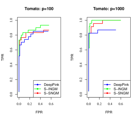
Figure 7: ROC curve for performance on tomato dataset

6 Discussion

In this paper, we propose NGMs for feature importance assessment and controlled selection in neural network models, which is an important aspect for model interpretation. Even in situations with no need of explicit feature selections, having a good rank of the predictors according to their influence on the output can be very helpful for practitioners to prioritize their follow-up work. We emphasize that our method does not require any distributional assumption on $\bm{X}$, thus is widely applicable to a broad class of neural network models including those with discrete or categorical features. In addition, the mirror design can be generated to convolutional neural networks (CNN) to measure the stability of the filters. For example, for each original CNN slice in the input tensor, we can create its corresponding mirrored slice by adding and subtracting a slice of random perturbations, and contrast the influences of the original and mirrored slices. detailed study in this direction is deferred to a future work. The data used in the real example is available in (ftp.solgenomics.net/manuscripts/Bauchet_2016/).

Supplementary materials

Appendix A Test statistics for conditional independence

To simplify the notations, let

$$(U,V,W)=(X_{j}^{+},X_{j}^{-},X_{-j})$$

Lemma A.1

$U$ and $V$ are conditional independent if and only if $\eta_{U,V}(u,v)+\eta_{U,V,W}(u,v,w)=0$

Proof

Suppose $f$ is the joint density function for $(U,V,W)=(X_{j}^{+},X_{j}^{-},X_{-j})$, then it can be decomposed into $2^{3}=8$ factors:

$$f(u,v,w) =\exp(\eta_{U}(u)+\eta_{V}(v)+\eta_{W}(w)$$

$$+\eta_{U,W}(u,w)+\eta_{V,W}(v,w)+\eta_{U,V}(u,v)$$

$$+\eta_{U,V,W}(u,v,w)),$$ (A.1)

where $\eta$ represents log-transformed density and $\eta_{A}(\alpha)$ means the part as the function only of $\alpha$. Then

$$\eta(u,v,w) =\eta_{U}(u)+\eta_{V}(v)+\eta_{W}(w)$$

$$+\eta_{U,W}(u,w)+\eta_{V,W}(v,w)+\eta_{U,V}(u,v)$$

$$+\eta_{U,V,W}(u,v,w)$$ (A.2)

To assess the dependence between $(U,V)$ conditioned on $W$, we derive the conditional density as

$$f_{(U,V|W)}(u,v|w)=\frac{e^{\eta(u,v,w)}}{\int_{\mathcal{U}}\int_{\mathcal{V}}e^{\eta(u,v,w)}}$$

$$=C(w)\cdot e^{\eta_{U}(u)+\eta_{U,W}(u,w)}\cdot$$

$$~{}~{}~{}e^{\eta_{V}(v)+\eta_{V,W}(v,w)}\cdot e^{\eta_{U,V}(u,v)+\eta_{U,V,W}(u,v,w)}$$ (A.3)

where $C(w)$ denotes the denominator as the marginal density of $W$. Therefore $U\perp\!\!\!\!\perp V|W$ if and only if any interaction of $U$ and $V$ is constants, i.e. $\eta_{U,V}+\eta_{U,V,W}=0.$ $\hfill\blacksquare$

Appendix B Importance measurement in DNN

In order to construct mirror statistics in DNNs, we first adopt an importance measure for each input feature.

We consider a fully connected multi-layer perceptron (MLP) with $k$ hidden layers denoted as $(H^{(t)}_{1},\dots,H^{(t)}_{n_{t}})$ for $t=1,\dots,k$. The output of the ($t+1$)-th layer can be described as

$$H_{j}^{(t+1)}=g_{t+1}(\sum_{i=1}^{n_{t}}w_{ij}^{(t)}H_{i}^{(t)}),\ \mbox{for }\ j=1,\dots,n_{t+1},$$

where $g_{t+1}$ is the activation function. Note that $t=0$ denotes the input layer and $t=k+1$ denotes the output layer.

We define

$$\delta(\bm{l}(X_{j},H_{i_{1}}^{(1)},...,H_{i_{k}}^{(k)},y))=\omega_{ji_{1}}^{(0)}\omega^{(k)}_{i_{k}1}\prod_{t=1}^{k-1}\omega^{(t)}_{i_{t}i_{t+1}}$$

as the accumulated weight of the path $\bm{l}$.

Let $\bm{\Omega}^{(0)}_{j}=(\omega_{j1}^{(0)},\dots,\omega_{jn_{1}}^{(0)})$ as the weight vector connecting $X_{j}$ with the first layer. We define the feature importance of $j$th feature as

$$L(X_{j})=\sum_{\bm{l}\in P_{j}}\delta(\bm{l})=\langle\bm{C},\bm{\Omega}^{(0)}_{j}\rangle,$$ (B.1)

where $P_{j}$ is the set consisting of all paths connecting $X_{j}$ to $y$ with one node in each layer and $\bm{C}=\prod_{t=1}^{k}\bm{\Omega}^{(t)}$, where $\bm{\Omega}^{(t)}_{ij}=\omega_{ij}^{(t)}\in\mathbb{R}^{n_{t}\times n_{t+1}}$ for $i=1,\dots,n_{t}$ and $j=1,\dots,n_{t+1}$.

For $t=1,\dots,k$, define diagonal matrices

$$\bm{G}^{(t)}={\rm diag}( \frac{\partial g_{t}}{\partial h}(\sum_{i=1}^{n_{t-1}}w_{i1}^{(t-1)}H_{i}^{(t-1)}),\dots,$$

$$\frac{\partial g_{t}}{\partial h}(\sum_{i=1}^{n_{t-1}}w_{in_{t}}^{(t-1)}H_{i}^{(t-1)})).$$ (B.2)

Then, the gradient w.r.t. $X_{j}$ can be written as

$$\frac{\partial y}{\partial X_{j}}=\bm{\Omega}^{(0)}_{j}\prod_{t=1}^{k}(\bm{G}^{(t)}\bm{\Omega}^{(t)}),$$ (B.3)

which is a weighted version of $L(X_{j})$.

Appendix C Perturbation with linear kernel

Suppose $n$ observations $(\bm{x}_{i},y_{i}),i=1,2,\dots,n$ are drawn from the model

$$y=\phi(\bm{x})^{\top}\bm{\beta}+\epsilon$$

where $\phi(\cdot)$ is a feature map and the kernel function $k(\cdot,\cdot)$ is define as

$$k(\bm{x},\bm{z})=\langle\phi(\bm{x}),\phi(\bm{z})\rangle$$

In the classical linear model $y=\bm{x}^{\top}\bm{\beta}+\epsilon$, $\phi$ is chosen to be the identity with a constant interception and thus $k(\cdot,\cdot)=\langle\cdot,\cdot\rangle+{\rm const}$.

To specify the test statistics when adopting linear kernels

$$[I_{j}^{K}(c)]^{2}$$

$$=\frac{1}{n^{2}}[(\bm{H}\bm{K}^{U}\bm{H})\circ(\bm{H}\bm{K}^{V}\bm{H})\circ\bm{K}^{W}]_{++}$$

$$=\frac{1}{n^{2}}\{[(\bm{H}U)(\bm{H}U)^{\top}]\circ[(\bm{H}V)(\bm{H}V)^{\top}]$$

$$~{}~{}~{}~{}~{}~{}\circ(WW^{\top})\}_{++}$$ (C.1)

where $(U,V,W)=(X_{j}^{+},X_{j}^{-},X_{-j})$ and $\bm{H}=I_{n}-\frac{1}{n}\mathbf{1}_{n}\mathbf{1}_{n}^{\top}$. To simplify notations, denote $U=\bm{H}U$ and $V=\bm{H}V$, with which

$$G(c)\triangleq n^{2}[I_{j}^{K}(c)]^{2}$$

$$=\{[(X_{j}+cZ_{j})(X_{j}+cZ_{j})^{\top}]$$

$$~{}~{}~{}~{}~{}~{}\circ[(X_{j}-cZ_{j})(X_{j}-cZ_{j})^{\top}]\circ(WW^{\top})\}_{++}.$$ (C.2)

We take gradient of $G(c)$ with respect to $c$ and due to the community of operators:

$$\nabla_{c}G(c)$$

$$=\{\frac{\partial}{\partial c}([(X_{j}+cZ_{j})(X_{j}+cZ_{j})^{\top}]$$

$$~{}~{}~{}~{}~{}~{}\circ[(X_{j}-cZ_{j})(X_{j}-cZ_{j})^{\top}])\circ(WW^{\top})\}_{++}$$

$$=\{\nabla_{c}[(X_{j}+cZ_{j})(X_{j}+cZ_{j})^{\top}]$$

$$~{}~{}~{}~{}~{}~{}\circ[(X_{j}-cZ_{j})(X_{j}-cZ_{j})^{\top}]\circ(WW^{\top})$$

$$~{}~{}~{}+[(X_{j}+cZ_{j})(X_{j}+cZ_{j})^{\top}]$$

$$~{}~{}~{}~{}~{}~{}\circ\nabla_{c}[(X_{j}-cZ_{j})(X_{j}-cZ_{j})^{\top}]\circ(WW^{\top})\}_{++}$$

$$=c\{[2c^{2}(Z_{j}Z_{j}^{\top})\circ(Z_{j}Z_{j}^{\top})+2(X_{j}X_{j}^{\top})\circ(Z_{j}Z_{j}^{\top})$$

$$~{}~{}~{}-(X_{j}Z_{j}^{\top})\circ(X_{j}Z_{j}^{\top})-(Z_{j}X_{j}^{\top})\circ(Z_{j}X_{j}^{\top})$$

$$~{}~{}~{}~{}~{}~{}-2(X_{j}Z_{j}^{\top})\circ(Z_{j}X_{j}^{\top})]\circ(WW^{\top})\}_{++}.$$ (C.3)

Therefore, $\nabla_{s}G(s)=0$ leads to the solution as follow:

$$c^{*}_{j}=\sqrt{\frac{\{A(X_{j},Z_{j})\circ(WW^{\top})\}_{++}}{2[(Z_{j}Z_{j}^{\top})\circ(Z_{j}Z_{j}^{\top})\circ(WW^{\top})]_{++}}},$$ (C.4)

with $A(X_{j},Z_{j})=(Z_{j}X_{j}^{\top})\circ(Z_{j}X_{j}^{\top})+(X_{j}Z_{j}^{\top})\circ(X_{j}Z_{j}^{\top})$. And $c_{j}^{*}$ is the minimum point by computing the second-order derivatives w.r.t. $c$.

For the space $span\{W\}$, let $P_{W}$ be the projection operator, then $c_{j}$ in the Gaussian Mirror can be written as

$$c_{j}^{\rm GM}=\sqrt{\frac{\|(I-P_{W})X_{j}\|^{2}}{\|(I-P_{W})Z_{j}\|^{2}}}.$$ (C.5)

We should note that, without the term $WW^{\top}$, $[(Z_{j}Z_{j}^{\top})\circ(Z_{j}Z_{j}^{\top})]_{++}=\|Z_{j}\|^{4}$, $[(Z_{j}X_{j}^{\top})\circ(Z_{j}X_{j}^{\top})]_{++}=[(X_{j}Z_{j}^{\top})\circ(X_{j}Z_{j}^{\top})]_{++}=\|X_{j}\|^{2}\|Z_{j}\|^{2}$. Therefore, comparing the form of C.4 and C.5, $c_{j}^{*}$ and $c_{j}^{\rm GM}$ are of the same scale which is validated in the simulation and they are equivalent with orthogonal designs.

Table 3: Linear Model with varying constant partial correlation(q=0.1)

$n=1000$	partial correlation	S-SNGM		SNGM		S-INGM		DeepPink
		FDR	Power	FDR	Power	FDR	Power	FDR	Power
$p=500$	$\rho=0$	0.064	0.910	0.083	0.907	0.060	0.890	0.135	0.907
	$\rho=0.2$	0.065	0.903	0.071	0.905	0.096	0.887	0.092	0.900
	$\rho=0.4$	0.068	0.902	0.012	0.815	0.080	0.898	0.094	0.913
	$\rho=0.6$	0.071	0.893	0.024	0.870	0.067	0.900	0.169	0.927
	$\rho=0.8$	0.076	0.880	0.008	0.838	0.103	0.882	0.168	0.907
$p=2000$	$\rho=0$	0.076	0.798	0.017	0.842	0.053	0.860	0.146	0.787
	$\rho=0.2$	0.053	0.808	0.058	0.873	0.062	0.850	0.058	0.740
	$\rho=0.4$	0.072	0.798	0.014	0.810	0.044	0.840	0.096	0.800
	$\rho=0.6$	0.083	0.805	0.048	0.812	0.063	0.810	0.125	0.767
	$\rho=0.8$	0.063	0.798	0.330	0.815	0.073	0.737	0.177	0.740

Appendix D Additional simulation results with varying correlation

Consider the linear model $y_{i}=\bm{\beta}^{\top}\bm{x}_{i}+\epsilon_{i},\ \epsilon_{i}\stackrel{{\scriptstyle\mbox{\small{i.i.d.}}}}{{\sim}}N(0,1)$, for $i=1,\dots,n$. We randomly set $k=30$ elements in $\bm{\beta}$ to be nonzero and generated from $\mathcal{N}(0,(20\sqrt{log(p)/n})^{2})$ to mimic various signal strengths in real applications. We set $n=1000$ and study both the low-dimensional case with $p=500$ and the high-dimensional case with $p=2000$ respectively.

As shown in the Table 3, S-SNGM and S-INGM have exact FDR control under $q=0.1$ and meanwhile have higher power than the DeepPINK. Besides, SNGM controls FDR under $q=0.1$ except for the case with $p=2000,\rho=0.8$ that is diffcult for mirror construction. In the high-dimensional setting with high partial correlation, DeepPINK undergoes an obvious power loss since the minimum eigenvalue of correlation matrix is $1/(1+(p-1)\rho)\approx 0$, which imposes great obstacles for the Knockoff construction, but NGM with screening procedure is more stable in power maintenance.

References

- [1] Reza Abbasi-Asl and Bin Yu. Interpreting convolutional neural networks through compression. arXiv preprint arXiv:1711.02329, 2017.
- [2] Rina Foygel Barber, Emmanuel J Candès, et al. Controlling the false discovery rate via knockoffs. The Annals of Statistics, 43(5):2055–2085, 2015.
- [3] Rina Foygel Barber, Emmanuel J Candès, et al. A knockoff filter for high-dimensional selective inference. The Annals of Statistics, 47(5):2504–2537, 2019.
- [4] Guillaume Bauchet, Stéphane Grenier, Nicolas Samson, Julien Bonnet, Laurent Grivet, and Mathilde Causse. Use of modern tomato breeding germplasm for deciphering the genetic control of agronomical traits by genome wide association study. Theoretical and applied genetics, 130(5):875–889, 2017.
- [5] Yoav Benjamini and Yosef Hochberg. Controlling the false discovery rate: a practical and powerful approach to multiple testing. Journal of the Royal statistical society: series B (Methodological), 57(1):289–300, 1995.
- [6] Yoav Benjamini, Daniel Yekutieli, et al. The control of the false discovery rate in multiple testing under dependency. The annals of statistics, 29(4):1165–1188, 2001.
- [7] Alain Berlinet and Christine Thomas-Agnan. Reproducing kernel Hilbert spaces in probability and statistics. Springer Science & Business Media, 2011.
- [8] Alexander Binder, Grégoire Montavon, Sebastian Lapuschkin, Klaus-Robert Müller, and Wojciech Samek. Layer-wise relevance propagation for neural networks with local renormalization layers. In International Conference on Artificial Neural Networks, pages 63–71. Springer, 2016.
- [9] Emmanuel Candès, Yingying Fan, Lucas Janson, and Jinchi Lv. Panning for gold:‘model-x’knockoffs for high dimensional controlled variable selection. Journal of the Royal Statistical Society: Series B (Statistical Methodology), 80(3):551–577, 2018.
- [10] Juan De Oña and Concepción Garrido. Extracting the contribution of independent variables in neural network models: A new approach to handle instability. Neural Comput. Appl., 25(3–4):859–869, September 2014.
- [11] Yingying Fan, Emre Demirkaya, Gaorong Li, and Jinchi Lv. Rank: large-scale inference with graphical nonlinear knockoffs. Journal of the American Statistical Association, pages 1–43, 2019.
- [12] Yingying Fan, Jinchi Lv, et al. Innovated scalable efficient estimation in ultra-large gaussian graphical models. The Annals of Statistics, 44(5):2098–2126, 2016.
- [13] Kenji Fukumizu, Arthur Gretton, Xiaohai Sun, and Bernhard Schölkopf. Kernel measures of conditional dependence. In Advances in neural information processing systems, pages 489–496, 2008.
- [14] Amirata Ghorbani, Abubakar Abid, and James Zou. Interpretation of neural networks is fragile. In Proceedings of the AAAI Conference on Artificial Intelligence, volume 33, pages 3681–3688, 2019.
- [15] Amir Globerson and Sam Roweis. Nightmare at test time: robust learning by feature deletion. In Proceedings of the 23rd international conference on Machine learning, pages 353–360. ACM, 2006.
- [16] Arthur Gretton, Karsten M Borgwardt, Malte J Rasch, Bernhard Schölkopf, and Alexander Smola. A kernel two-sample test. Journal of Machine Learning Research, 13(Mar):723–773, 2012.
- [17] Chong Gu. Smoothing spline ANOVA models, volume 297. Springer Science & Business Media, 2013.
- [18] Yotam Hechtlinger. Interpretation of prediction models using the input gradient. arXiv preprint arXiv:1611.07634, 2016.
- [19] Geoffrey E Hinton and Ruslan R Salakhutdinov. Reducing the dimensionality of data with neural networks. science, 313(5786):504–507, 2006.
- [20] Dongming Huang and Lucas Janson. Relaxing the assumptions of knockoffs by conditioning. arXiv preprint arXiv:1903.02806, 2019.
- [21] Yi Lin et al. Tensor product space anova models. The Annals of Statistics, 28(3):734–755, 2000.
- [22] Yang Lu, Yingying Fan, Jinchi Lv, and William Stafford Noble. Deeppink: reproducible feature selection in deep neural networks. In Advances in Neural Information Processing Systems, pages 8676–8686, 2018.
- [23] Avanti Shrikumar, Peyton Greenside, and Anshul Kundaje. Learning important features through propagating activation differences. In Proceedings of the 34th International Conference on Machine Learning-Volume 70, pages 3145–3153. JMLR. org, 2017.
- [24] Nitish Srivastava, Geoffrey Hinton, Alex Krizhevsky, Ilya Sutskever, and Ruslan Salakhutdinov. Dropout: a simple way to prevent neural networks from overfitting. The journal of machine learning research, 15(1):1929–1958, 2014.
- [25] John D Storey, Jonathan E Taylor, and David Siegmund. Strong control, conservative point estimation and simultaneous conservative consistency of false discovery rates: a unified approach. Journal of the Royal Statistical Society: Series B (Statistical Methodology), 66(1):187–205, 2004.
- [26] Ryan Turner. A model explanation system. In 2016 IEEE 26th International Workshop on Machine Learning for Signal Processing (MLSP), pages 1–6. IEEE, 2016.
- [27] Antanas Verikas and Marija Bacauskiene. Feature selection with neural networks. Pattern Recognition Letters, 23(11):1323–1335, 2002.
- [28] Pascal Vincent, Hugo Larochelle, Yoshua Bengio, and Pierre-Antoine Manzagol. Extracting and composing robust features with denoising autoencoders. In Proceedings of the 25th international conference on Machine learning, pages 1096–1103. ACM, 2008.
- [29] Stefan Wager, Sida Wang, and Percy S Liang. Dropout training as adaptive regularization. In Advances in neural information processing systems, pages 351–359, 2013.
- [30] Sida Wang and Christopher Manning. Fast dropout training. In international conference on machine learning, pages 118–126, 2013.
- [31] Xin Xing, Zhigen Zhao, and Jun S. Liu. Controlling false discovery rate using gaussian mirrors. Technical Report, 2019.
- [32] Méziane Yacoub and Younès Bennani. Hvs : A heuristic for variable selection in multilayer artificial neural network classifier. 1997.
- [33] Bin Yu et al. Stability. Bernoulli, 19(4):1484–1500, 2013.
- [34] Bin Yu and Karl Kumbier. Three principles of data science: predictability, computability, and stability (pcs). arXiv preprint arXiv:1901.08152, 2019.