Cut-and-Paste Object Insertion by Enabling Deep Image Prior for Reshading

Abstract

We show how to insert an object from one image to another and get realistic results in the hard case, where the shading of the inserted object clashes with the shading of the scene. Rendering objects using an illumination model of the scene doesn’t work, because doing so requires a geometric and material model of the object, which is hard to recover from a single image. In this paper, we introduce a method that corrects shading inconsistencies of the inserted object without requiring a geometric and physical model or an environment map. Our method uses a deep image prior (DIP), trained to produce reshaded renderings of inserted objects via consistent image decomposition inferential losses. The resulting image from DIP aims to have (a) an albedo similar to the cut-and-paste albedo, (b) a similar shading field to that of the target scene, and (c) a shading that is consistent with the cut-and-paste surface normals. The result is a simple procedure that produces convincing shading of the inserted object. We show the efficacy of our method both qualitatively and quantitatively for several objects with complex surface properties and also on a dataset of spherical lampshades for quantitative evaluation. Our method significantly outperforms an Image Harmonization (IH) baseline for all these objects. They also outperform the cut-and-paste and IH baselines in a user study with over 100 users.

1 Introduction

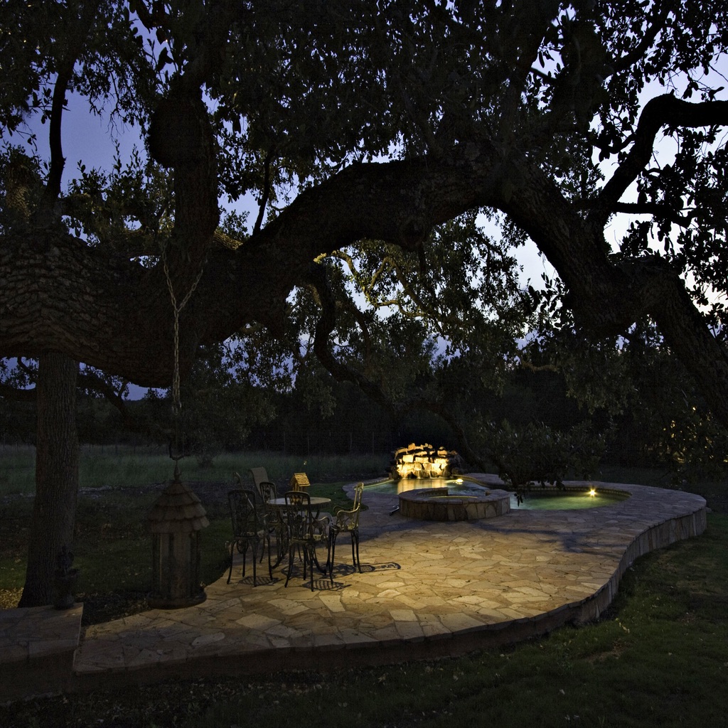
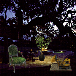
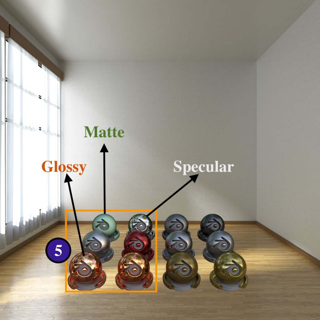
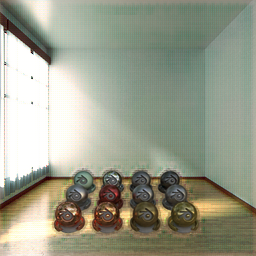
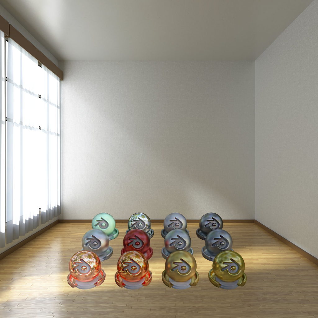
Target Scene	Cut-and-Paste (CP)	Image Harmonization (IH) [9]	DIPR (ours)

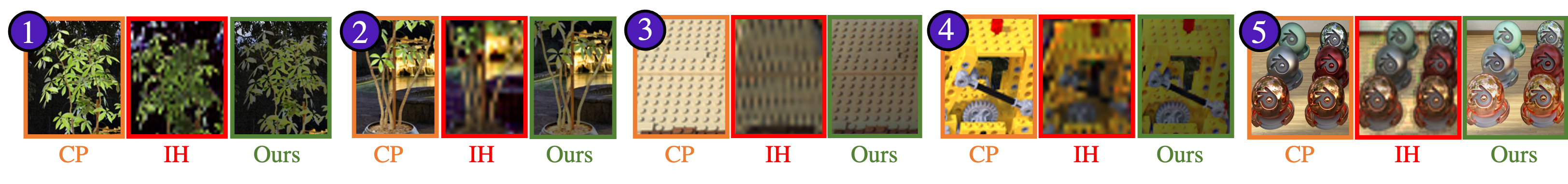
Figure 1: We synthesize realistic, high-resolution renderings of objects added to scenes – cut from one image and pasted into another. Our approach, DIPR, is entirely image-based and can convincingly insert objects with complex surface properties (a lego dozer, a plant and a chair in the first row) and matte, glossy and specular objects (a set of 16 different materials in the second row; crop$\#5$ in bottom row) added to spatially varying illuminating scenes (indoor-outdoor, day-night) without requiring the geometry of the inserted objects or the parameters of the target scene. Key findings from our method are (a) it appears to handle complex and subtle interaction with light; for eg., leaves (crop$\#1$) (b) it appears to understand 3D scene and illumination reasonably well (crop$\#2$); CP in crop$\#2$ looks realistic in local context, but it isn’t capturing the 3D scene – the light source behind is far away from the plant, and (c) it preserves material properties because of a carefully designed model; enabling object insertion without any loss of high-frequency details (crop$\#3\ \&\ \#4$).

Inserting objects into images is an appealingly easy rendering paradigm – one just moves objects from one image into another. Applications of this task are abundant, ranging from room planners to image editing for artists to training detectors [33, 11]. But most insertions are not realistic because the shading between the inserted object clashes with the target scene and the object sticks out [23]. Current state-of-the-art (SOTA) methods recover an environment map and render objects using their geometric and physical model [29, 15]. Current single-image methods for shape and material recovery cannot accurately reconstruct realistic objects (say, a lego toy) [32]. Therefore, in this work, we focus on an image-based insertion approach: one takes an object from one image, inserts it into another, and expects a system to correct it. Our method not only synthesizes plausibly realistic renderings of inserted objects with complex surface properties but also does not require a geometric or physical model or an environment map at test time. Furthermore, it does not require rendered images during training.

Our method, DIPR, uses Deep Image Prior [54] for reshading. DIPR adjusts shading so that simple inferences are consistent with cut-and-paste predictions. The rendering process produces an image that is realistic, guaranteed by our use of a deep image prior. The rendering must also produce (a) an albedo that matches the cut-and-paste albedo, (b) a shading that matches the target scene’s shading outside the inserted fragment, and (c) the rendered shading and the cut-and-paste normals are consistent with each other. The result is a simple procedure that produces convincing shading. Our entire process, including image decomposition, does not require any form of labeled data for training. We use an extension of Retinex[26], build a statistical process for data generation and train variants of image decomposition models for DIPR. In fact, our only use of simulated ground truth is our use of a pre-trained, off-the-shelf, normal estimator [41].

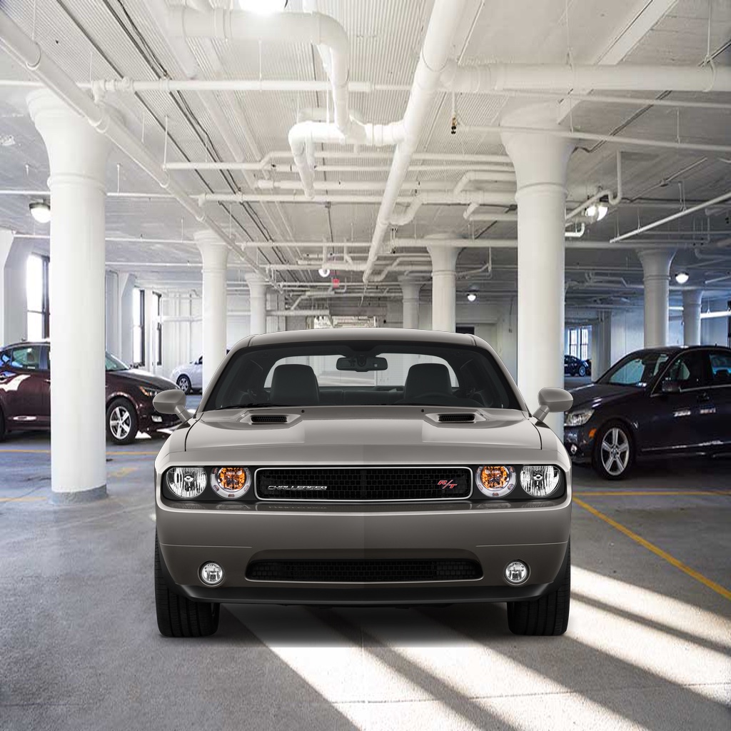
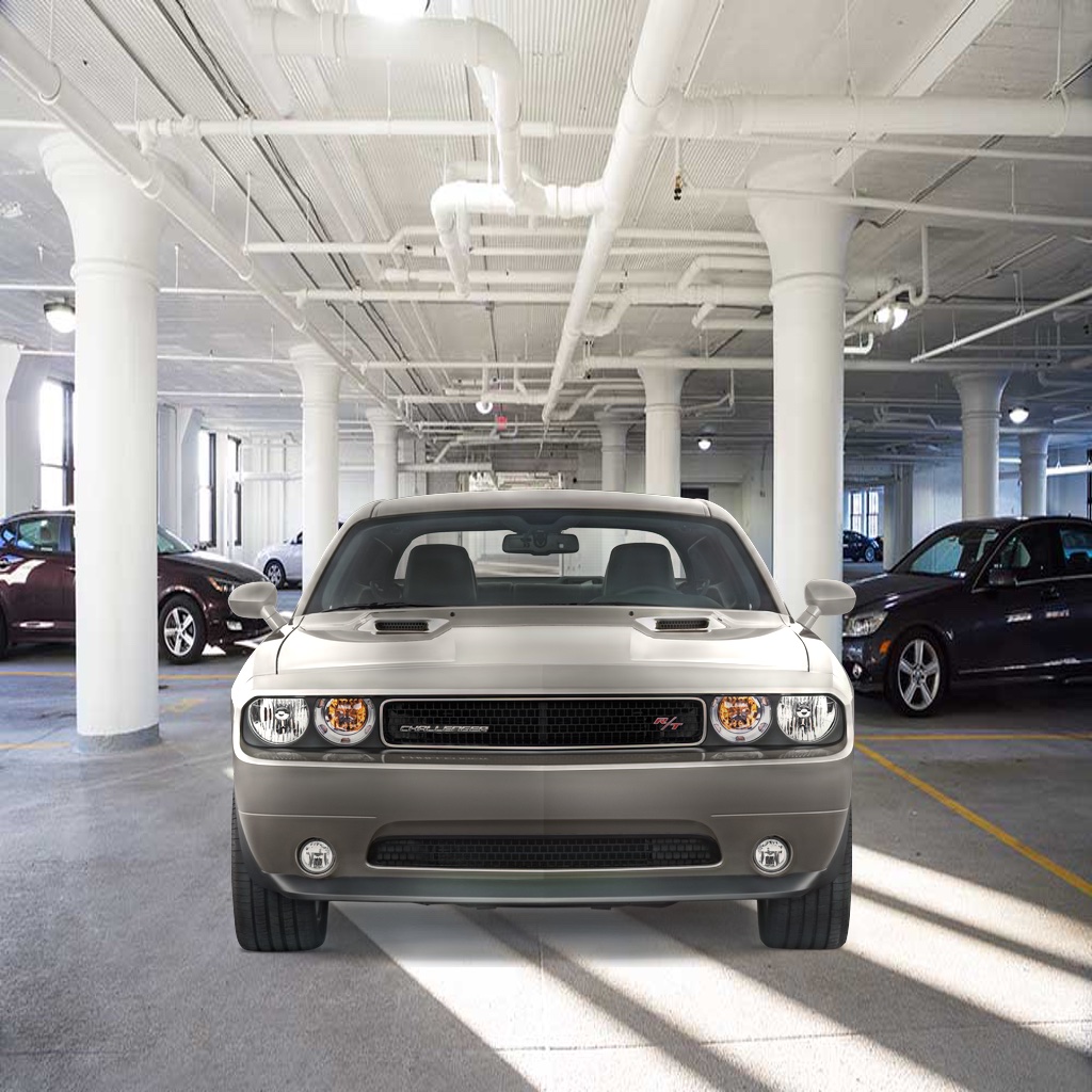
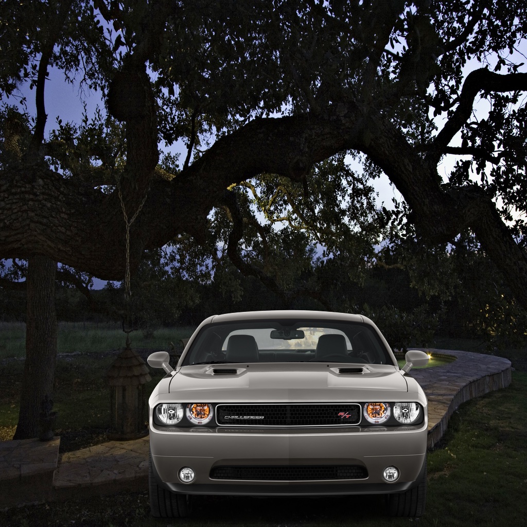
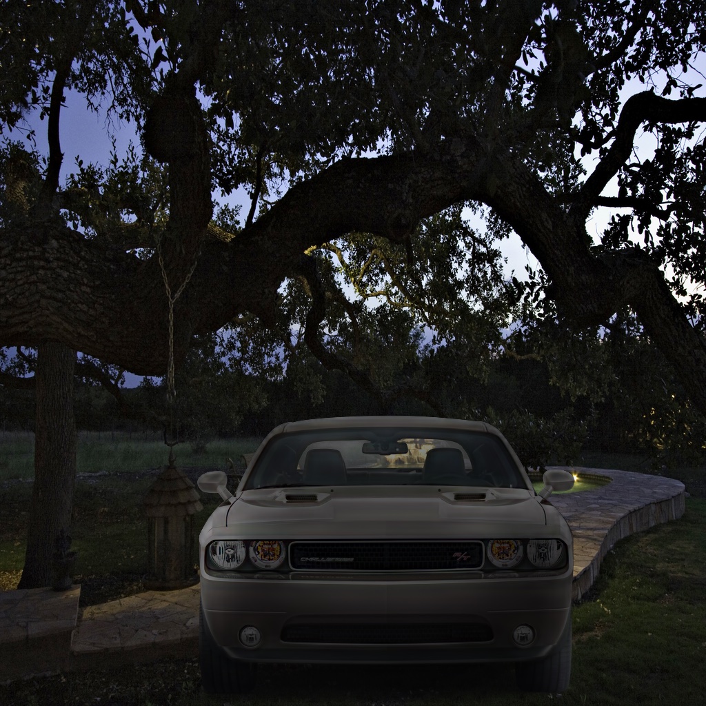
Target Scene	CP	IH [9]	DIPR (ours)

Figure 14: Additional examples of reshading real cars. Glossy effects in car paint with glitter in them make reshading cars a particularly challenging case with their complex reflective properties. DIPR successfully reshades cars without a distinct shift in object and background color produced by IH. Note the bright patch on the metallic bonnet of the grey car in the top row that may possibly be because of the light source just above it.

Our experiments show DIPR convincingly inserts several objects with complex surface properties – a lego dozer, a plant, a chair and a set of 16 materials with different reflective properties (Fig. 1), cars (Fig. 14) and spherical lampshades (Fig. 6). In qualitative analysis, we show DIPR produces convincing results compared to a SOTA image harmonization baseline [9]. We also find that DIPR achieves significantly better PSNR, MSE and LPIPS scores, outperforming a SOTA image harmonization baseline for lampshades renderings (Tab. 1). We conduct user studies comparing our renderings against baselines and real images. We also show our method has an implicit notion of 3D shape as an emergent property of our consistent reshading (Fig. 10).

In summary, our main contributions are (1) we enable deep image priors to explicitly reason about the shading of the scene by a new class of image decomposition model. (2) Our method can realistically insert objects without any ground truth labeled data. The only labeled data that our method requires is a surface normal, obtained from a pretrained network. Other than that, our method is completely self-supervised. (3) Our method works for matte, glossy and specular objects with complex surface properties and without using explicit geometric or physical model of the scene. (4) Our method works for diverse (indoor-outdoor, day-night) spatially varying illuminated complex scenes. (5) Our method produces convincing results compared to a SOTA image harmonization baseline and achieves significantly better PSNR, MSE and LPIPS scores. (6) Our method has an implicit notion of 3D shape as an emergent property of our consistent reshading.

2 Related Work

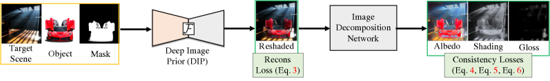
Figure 2: DIPR overview. DIPR generates a plausibly realistic rendering of an object inserted from a source image to a target scene. DIPR uses a DIP to generate a reshaded rendering that has consistent image decomposition inferences. The resulting rendering from DIP should have an albedo, same as the cut-and-paste albedo; it should have a shading and gloss field that, outside the inserted fragment, is the same as the target scene’s shading and gloss field. The rendering must have similar spherical harmonic properties as target scene and meet a consistency test everywhere (Sec 3.4, Fig. 5). This simple procedure inserts objects convincingly in real images.

Object insertion originated with Lalonde et al. [23]. They insert objects into target images and control illumination problems by checking objects for compatibility with targets; Bansal et al. [1] and Lee et al. [28] do so by matching contexts. Poisson blending [43, 20] can resolve nasty boundary artifacts, but significant illumination and color mismatches will cause cross-talk between target and fragment, producing ugly results. Karsch et al. [21, 22] how convincing insertions of computer graphics (CG) objects into inverse rendering models. Inverse rendering trained with rendered images can produce excellent reshading of CG objects [45]. However, recovering a renderable model from an image fragment is extremely difficult, particularly if the fragment has an odd surface texture. Liao et al.[34, 35] showed that a weak geometric model of the object can be sufficient for correcting shading if one has strong the geometric information about the target scene. However, we do not know about geometry of the target scene, except for their normals.

We use image harmonization (IH) methods as a strong baseline. IH train models to correct corrupted images where a fragment is adjusted by some noise process (made brighter; recolored; etc.) to the original image [52, 53, 9, 37, 18], and so could clearly be applied here. But we find those IH methods very often change the albedo of an inserted object, rather than its shading. This is because they rely on ensuring consistency of color representations across the image. In contrast, we wish to correct shading alone.

Image Relighting: With appropriate training data, for indoor-scenes, one can predict multiple spherical harmonic components of illumination [15], or parametric lighting model [14] or even full radiance maps at scene points from images [49, 50]. For outdoor scenes, the sun’s position is predicted in panoramas using a learning-based approach [19]. However, we do not have access to either training data with lighting parameters/environment maps to construct such a radiance field. Recent single-image relighting methods relight portrait faces under directional lighting [51, 59, 42]. Our method can relight matte, gloss and specular objects with complex material properties like cars (Fig. 14) for both indoor and outdoor spatially varying lighting only from a single image and without requiring physics-based BRDF [29].

Land’s Retinex (image decomposition) model assumes effective albedo displays sharp, localized changes (which result in large image gradients), and that shading has small gradients [24, 25, 26, 27]. These models require no ground truth. An alternative is to use CG rendered images for training [30, 6, 12]. Current image decomposition evaluation uses the weighted human disagreement rate (WHDR) [4]; current champions are [12, 13]. We use an image decomposition built around approximate statistical models of albedo and shading [13] to train our network without requiring real image decompositions. Our method has reasonable, but not SOTA, WHDR; but we show that improvements in WHDR do not result in improvements in reshading (Fig. 3).

3 Approach

DIPR synthesizes a reshaded object transferred from the source image ($s$) into a target scene image ($t$). We use a deep image prior (DIP) [54] as a renderer to produce a reshaded image. We enable DIP to reshade by forcing it to produce consistent image decomposition inferences that meet certain shading consistency tests. We use an image decomposition trained on statistical samples of albedo, shading and gloss; Fig. 4a and not real images (Sec 3.2), and surface normals inferred by the method of [41] to meet the shading consistency tests (Sec 3.4). The final reshaded image’s albedo must be like the cut-and-paste albedo; the reshaded image’s shading must match the shading of the target scene outside the fragment; and the shading of the reshaded image must have reasonable spherical harmonic properties and meet a consistency test everywhere Fig. 2 summarizes our method.

3.1 Enabling DIP for object reshading

Assume we have a noisy image ${I}_{t}$, and wish to reconstruct the original. Write $z$ for a random vector, and $f_{\theta}$ for a CNN with parameters $\theta$ and $E(f_{\theta}(z);{I}_{t})$ for a loss comparing the image $f_{\theta}(z)$ to ${I}_{t}$. DIP seeks

$$\hat{\theta}=\mbox{argmin}_{\theta}E(f_{\theta}(z);{I}_{t})$$ (1)

and then reports $f_{\hat{\theta}}(z)$. In this naive setup we find that the DIP always converges to cut-and-paste image. This is because the inconsistency we observe in cut-and-paste images are subtle view-dependent lighting effects that are difficult to capture using a simple DIP.

An alternative strategy is to decompose image into two components – a persistent map, one that is invariant to lighting effects and a transient map, one that changes with lighting. We then have to train a DIP only to make corrections to the extrinsic map and use intrinsic map as it is. To this end, we modify Eq. 1 by requiring that $E(\cdot;{I}_{t})$ only to adjust the extrinsic properties of the inserted object. In particular, write $g_{\phi}$ for some inference network(s), $t_{\psi}({I}_{s},{I}_{t})$ for inferences constructed out of ${I}_{t}$ and the source image ${I}_{s}$. DIPR seeks

$$\hat{\theta}=\mbox{argmin}_{\theta}E(g_{\phi}(f_{\theta}(z));t_{\psi}({I}_{s},{I}_{t})).$$ (2)

For us, $g_{\phi}$ is an image decomposition network, which is pretrained and fixed.

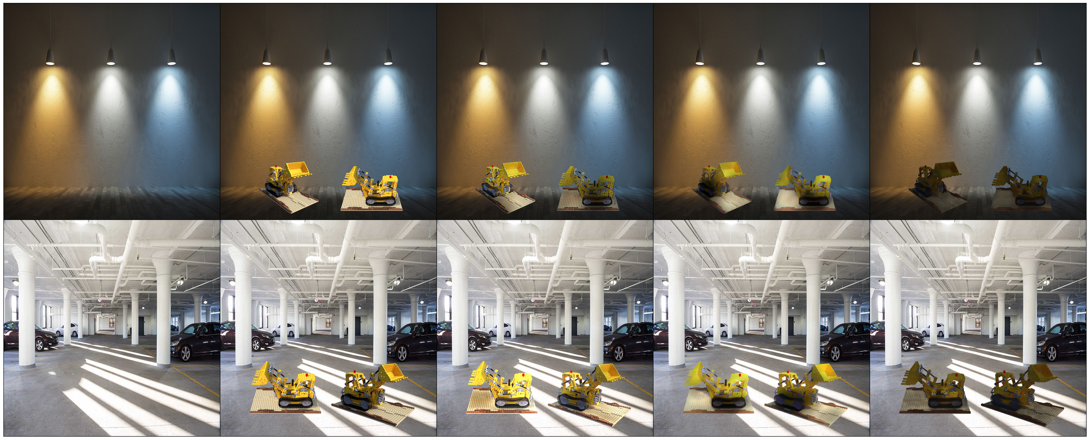
Target  Scene

CP

Our Decomposition

Paradigms [13]

CGIntrinsics[30]

Figure 3: Better WHDR does not mean better reshading. We show reshaded images when using target inferences from different decomposition models. Our decomposition achieves (relatively weak) WHDR of $19\%$; Paradigms [13] achieve $17\%$, and a supervised SOTA [30] achieve $15\%$. Paradigm  [13] decomposition produces worse reshading. Moreover, reshading using a supervised SOTA, CGIntrinsics[30], is worse than ours and Paradigms decomposition. This reflects that better recovery of albedo, as measured by WHDR, does not produce better reshading. The key issue is that methods that get low WHDR do so by suppressing small spatial details in the albedo field (for example, the surface detail on the lego dozer), and the shading inference method cannot recover these details, and so they do not appear in the final rendering. From the perspective of reshading, it is better to model them as fine detail in albedo than in shading.

3.2 Image Decomposition

A natural choice for an image decomposition is an albedo map (persistent to lighting) and a shading map (transient to lighting). One could then use a SOTA pretrained image decomposition network as $g_{\phi}$ only to adjust the shading of the scene and use the cut-and-paste albedo as it is. Next, we train DIP to reshade (DIPR) the inserted object to produce an image with their albedo, same as the cut-and-paste albedo and a shading field, same as the cut-and-paste image only for the background region other than the inserted fragment. DIPR then learns to extrapolate or interpolate shading for the inserted fragment from the background’s shading field.

We first evaluated DIPR with two SOTA image decomposition methods (one supervised [30] and one unsupervised [13]) as measured by strong WHDR performance. The supervised decomposition train their models on CG-generated datasets with ground-truth supervision. [13] uses Paradigms, a statistical model of albedo and shading, an extension of the Retinex [26]. Albedo paradigms are Mondrian images. Shading paradigms are Perlin noise [44]. We show these methods result in poor reshading outcomes (Fig  3). SOTA albedo-shading decompositions get strong WHDR performance by suppressing fine spatial details in albedo. These methods preserve spatial and geometric details in the shading field and not albedo because they construct albedo as a piece-wise color constant (Mondrian) with no fine details on them. These fine geometric details are hard to recover accurately from a DIP when trained to interpolate the foreground shading field from their background. However, [13] offers an interesting feature in their Paradigms construction. The statistical models used are authored. Changing the statistical properties of their models would result in a different class of decompositions. We take advantage of this feature. We change [13] and construct an albedo ($A$) – a persistent map, a diffuse shading ($S$) – a multiplicative transient map and a gloss ($G$) – an aditive transient map using the same statistical process. We compose them as $I=A\times S+G$ to form an image and train a network to decompose them back. Fig. 4a shows samples of our. Fig. 4b illustrates the resulting decompositions are satisfactory on MSCOCO [36] real images. The main difference between ours and  [13] is that we assume shading to be smooth and albedo has all the high-frequency information so that they can be recovered when reshading with a DIP. This is a reasonable assumption for our method because we aim to preserve all the fine-spatial details of inserted fragment when transferring from one image to another. The additional gloss map that we use helps us to extract better lighting representations in scenes with strong lighting effects like shafts. We show our decomposition produces convincing object reshading when compared to other SOTA image decomposition methods (Fig. 3).

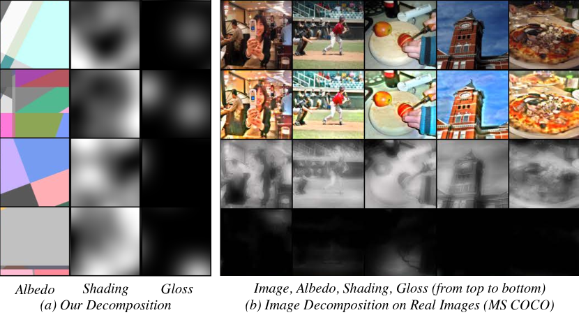
Figure 4: Image decomposition. Left: samples of our albedo, shading and gloss used to train our image decomposition network. Right: examples showing MS COCO image decompositions.

3.3 Base Losses

We first construct the desired target albedo ($A_{t}$), target shading and gloss ($S_{t}$ and $G_{t}$). We then train DIPR to produce an image that has reasonable albedo, shading and gloss properties. For DIPR, the input $z$ is the cut-and-paste image and $f_{\theta}$ is optimized to inpaint inserted fragment and also to meet satisfactory image decomposition consistency tests. We use U-Net with partial convolution [38, 48]. However, we find the standard partial convolution converges to a trivial solution, producing images close to cut-and-paste. To prevent this overfitting, we flip the context for partial convolution. We consider the inserted object(s) as the context and hallucinate/outpaint the entire target scene around it. We call this flipped partial convolution. This encourages the network not to overfit to the input cut-and-paste image.

We use ${CP}({I}_{s};{I}_{t};s)$ for an operator that cuts the fragment out of the source image (${I}_{s}$), scales it by $s$, and places it in the relevant location in the target image (${I}_{t}$). ${M}$ for a mask with the size of the target image that is $0$ inside the fragment and $1$ outside. Our reconstruction loss for the background is:

$$\small\mathcal{L}_{recons}={\mid\!\mid\!\!{{I}_{t}{\odot}{M}-(f_{\theta}({CP}({I}_{s};{I}_{t};s);{M}))}\!\!\mid\!\mid^{2}}$$ (3)

We then pass the DIP rendered image through the image decomposition network $g_{\phi}$ making $A_{r}$, $S_{r}$ and $G_{r}$ for the rendered albedo, shading and gloss maps respectively. Our consistent image decomposition inference losses to train DIPR are:

$$\mathcal{L}_{decomp}={\mid\!\mid\!\!{A_{{CP}({I}_{s};{I}_{t};s)}-A_{r}}\!\!\mid\!\mid^{2}}+{\mid\!\mid\!\!{S_{t}{\odot}{M}-S_{r}{\odot}{M}}\!\!\mid\!\mid^{2}}\\ +{\mid\!\mid\!\!{G_{t}{\odot}{M}-G_{r}{\odot}{M}}\!\!\mid\!\mid^{2}}$$ (4)

3.4 Normal Consistency Losses

We use two normal consistency losses to make the strong structure of a shading field apparent to a DIP’s reshading. There is good evidence that shading (image extrinsic)is tied across surface normals (this underlies spherical harmonic models [32, 56]), and one should think of a surface normal as a latent variable that explains shading or extrinsic similarities. We assume the resulting illumination approximated with the first 9 spherical harmonics basis coefficients ($Y$) and does not change when an object is inserted into a scene. We get $Y$ by solving the least square regression between normals (${N}$) and shading ($S$) for both the target scene and the resulting composite image. We then minimize loss ($\mathcal{L}_{Y}$) between the target and rendered image $Y$($S;{N}$) and use a Huber loss.

$$\centering\small\mathcal{L}_{Y}={\begin{cases}{\frac{1}{2}}({Y}(S_{t};{{N}}_{t})-{Y}(S_{r};{{N}_{CP}}))^{2}&{\textrm{for}}|Y_{t}-Y_{r}|\leq 1,\\ |{Y}(S_{t};{{N}}_{t})-{Y}(S_{r};{{N}_{CP}})|-{\frac{1}{2}}&{\textrm{otherwise.}}\end{cases}}\@add@centering$$ (5)

Spherical harmonic shading fields have some disadvantages: every point with the same normal must have the same shading value, which results in poor models of (say) indoor shading on walls. To control this effect, we use a novel neural shading consistency loss ($\mathcal{L}_{Z}$) that allows the shading field to depart from a spherical harmonic shading field, but only in ways consistent with past inferences. Our shading consistency discriminator, $\zeta(S;{N})$, is a U-Net [47] (Fig. 5); trained to discriminate real and fake shading-normal pairs. $\zeta(S;{N})$ produces two outputs: one a pixel-level map, yielding the first loss term in Eq. 6, which measures per-pixel consistency; the other an image-level value, the second term in Eq. 6, which measures consistency for the entire image. The $\mathcal{L}_{Z}$ loss is a binary cross-entropy loss. Let $m\times n$ be the resolution of our renderings, then $\mathcal{L}_{Z}$ is given by

$$\small\centering\mathcal{L}_{Z}=-\sum_{i=1}^{m}\sum_{j=1}^{n}\log\zeta(S_{r}[i,j];{N}_{{C}{P}}[i,j])-log\zeta(S_{r}{{N}_{CP}})\@add@centering$$ (6)

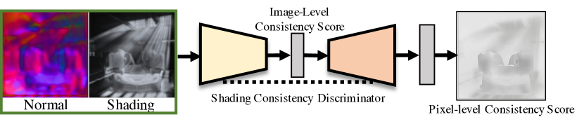
Figure 5: Shading consistency discriminator penalizes shading, if it is not consistent with the cut-and-paste normals.

In summary, we update DIPR with

$$\small\centering\mathcal{L}_{r}=\mathcal{L}_{recons}+\mathcal{L}_{decomp}+\mathcal{L}_{Y}+\mathcal{L}_{Z}\@add@centering$$ (7)

4 Experiments

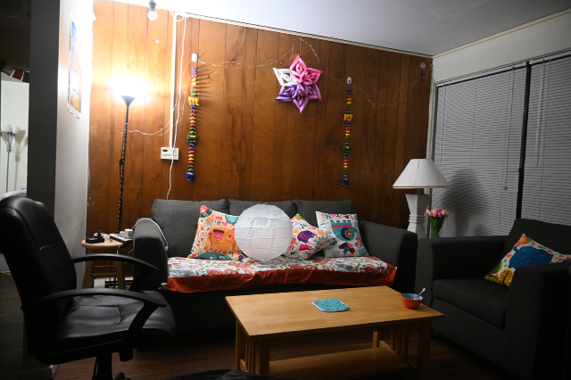
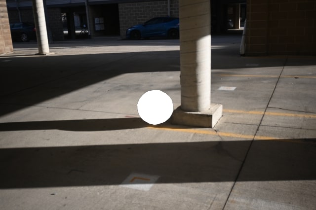
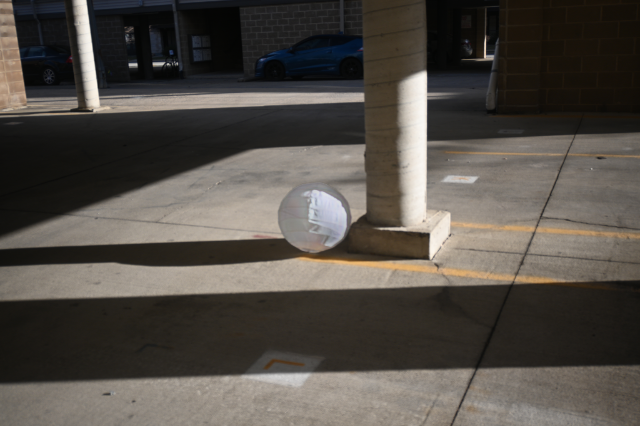
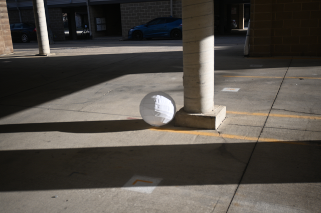
CP	IH [9]	DIPR (ours)	Real Scene

Figure 6: Reshading spherical lampshades. Similar to Fig. 9, we generate sphere rendering by overlaying 2D white disks over the real sphere from the photograph. We then use DIPR to reshade the overlaid 2D disk and combine that with the actual albedo (as they remain same irrespective of lighting) into a final rendering. IH copies average color. Our renderings are close to the ground truth (also see Tab. 1).

Scenes and objects. We collected about $100$ diverse images with spatially varying illumination, both indoors-outdoors, day-night, to act as target scenes in our experiments. $25$ of these scenes are captured by placing a spherical lampshade, which we use as ground truth for quantitative evaluation. We first test DIPR by inserting simple 2D bright disks at various locations in target scenes (Fig. 9). We also show reshading results for real cars inserted into our target scenes (Fig. 14). We also tested DIPR with complex surface properties – a lego dozer, a plant, a chair, and a set of sixteen materials with different reflective properties used in NeRF [39] (Fig. 1). Other objects from [32] are in our Appendix. We use ADE20K validation set [58] for supplying real residual loss to our image decomposition network and also to train our shading consistency network. ADE20K does not have ground truth normals and we use normals from [41].

Network architecture. Our DIP network is very similar to the U-Net used in 3DPhotoInpainting [48]. We use their provided model in our implementation as DIP. The only difference is our use of flipped partial convolution instead of standard partial convolution as described in our Sec 3.

Training details. We used U-Net for DIP, Image Decomposition and Shading Consistency Network. Network architecture and other training details are in our supplementary. We update our DIP for a fixed $10$k iterations and this takes about $900$ seconds using our image decomposition network and $1600$ seconds when using CGIntrinsic [30].

IH baseline. We use Cong et al.’s DoveNet [9] and their provided pretrained model for our IH baseline.

Quantitative comparison to ground truth. We compare 25 photographs of a spherical lampshade with DIPR based insertions. We get insertions by placing a white disk over the lampshade, reshading the disk using DIPR, then multiplying by lampshade’s albedo (a favorable case as it correctly rendered cast shadows). We then quantitatively compare results with ground truth (the real lampshade) using PSNR, LPIPS or MSE (Tab. 1; Fig. LABEL:fig:teaser, Fig. 6). Fig. LABEL:fig:teaser (b) and (c) are real.

Table 1: Quantitative Evaluation on Spherical Lampshades (Fig. 6). Cases: fixed shading fields ($S$ is constant); fixed albedo fields ($A$ constant); cut-and-paste albedo fields ($A_{{CP}({I}_{s};{I}_{t};s)}$); image harmonization (IH); and our reconstruction ($S_{r}$). Note DIPR reshading wins in all metrics. Note such comparisons to ground truth occur in circumstances favorable to a method like ours (because the shading around the object is consistent), but we know of no way to avoid this.

Shading ($S$)	Albedo ($A$)	LPIPS[57] $\downarrow$	PSNR $\uparrow$
$1$	$1$	$0.0105$	$30.81$
$S{{}_{r}}$	$1$	${0.0070}$	${34.26}$
DoveNet [9]	$A_{{CP}({I}_{s};{I}_{t};s)}$	${0.0072}$	${35.57}$
RainNet [37]	$A_{{CP}({I}_{s};{I}_{t};s)}$	${0.0070}$	${36.10}$
Harmony Transformer [18]	$A_{{CP}({I}_{s};{I}_{t};s)}$	${0.0069}$	${36.52}$
$0.25$	$A_{{CP}({I}_{s};{I}_{t};s)}$	$0.0113$	$26.74$
$0.50$	$A_{{CP}({I}_{s};{I}_{t};s)}$	$0.0060$	$31.28$
$0.75$	$A_{{CP}({I}_{s};{I}_{t};s)}$	0.$0032$	$38.18$
$1.0$	$A_{{CP}({I}_{s};{I}_{t};s)}$	0.$0043$	$36.66$
$S_{r}$ (ours)	$A_{{CP}({I}_{s};{I}_{t};s)}$	$\bf{0.0021}$	$\bf{39.53}$

Table 2: Ablation over losses show each helps improve reshading.

${\cal L}_{decomp}$(Eq. 4)	$\cal{L}_{Y}$ (Eq. 5)	$\cal{L}_{Z}$(Eq. 6)	LPIPS[57] $\downarrow$	PSNR $\uparrow$
✓			$0.0026$	$37.89$
✓		✓	${0.0023}$	${38.74}$
✓	✓		${0.0022}$	${39.09}$
✓	✓	✓	$\bf{0.0021}$	$\bf{39.53}$

Fooling users. The gold standard evaluation here is user studies (after all, the goal is to fool people). However, user studies are a poor way to polish a method, and a proxy would be valuable. For images of the spherical lampshade used in the quantitative evaluation of Tab. 1, we asked users to identify which of the two presented images (showing distinct scenes, but both containing the lampshade) was real. One image presented was always a rendering, the other always real. Users each see 16 pairs, and there were $72$ participants performing this study. Our DIPR renderings are very good at fooling users ($50\%$ is a chance). They pick DIPR $42.7\%$ of the time. We then use logistic regression to predict each rendered image’s probability of being marked real against MSE, PSNR and LPIPS. An accurate regression would mean that we had a score of “realness”. However, such a model explains almost none of the variation of the data (null deviance: $17.87$, residual deviance: $17$). This means that, while it is pleasant that DIPR has strong MSE, PSNR, and LPIPS scores, these scores can not be used to predict user preferences for our task.

For other object when we did not have ground truth for objects like cars, lego dozer, plant and chair, we conducted another user study to compare DIPR, CP, and IH renderings. Each study comprises a pre-qualifying process, followed by $9$ pair-wise comparisons, where the user is asked which of two images are more realistic. The result is $109$ pre-qualified studies. The comparisons are balanced. Each study is $3$ DIPR-IH pairs, $3$ CP-IH pairs, and $3$ DIPR-CP pairs, in random order.

We collected data from a total of 122 unique users in 500 studies from Amazon Mechanical Turk. Each study consists of a prequalifying process, followed by 9 pair-wise comparisons, where the user is asked which of two images are more realistic. The prequalifying process presents the user with five tests; each consists of an image with inserted white spheres which are not reshaded (i.e. bright white disks) and an image with inserted spheres which have been reshaded (see Fig 9). We ignore any study where the user does not correctly identify all five reshaded images, on the grounds that the difference is very obvious and the user must not have been paying attention.

The simplest analysis strongly supports DIPR is preferred over both alternatives. One compares the probability that DIPR is preferred to IH ($.673$, over $327$ comparisons, so standard error is $.026$, and the difference from $0.5$ is clearly significant); DIPR is preferred to CP ($.645$, over 327 comparisons, so the standard error is $.026$, and the difference from $0.5$ is clearly significant); IH is preferred to CP ($.511$, over $327$ comparisons, so standard error is $.027$, and there is no significant difference from $0.5$). An alternative is a Bradley-Terry model [53, 9] used in IH evaluation, regressing the quality predicted by the Bradley-Terry model against the class of algorithm. This yields coefficients of $0$ for IH, $-0.347$ for CP, and $0.039$ for DIPR, implying again that DIPR is preferred over IH and strongly preferred over CP.

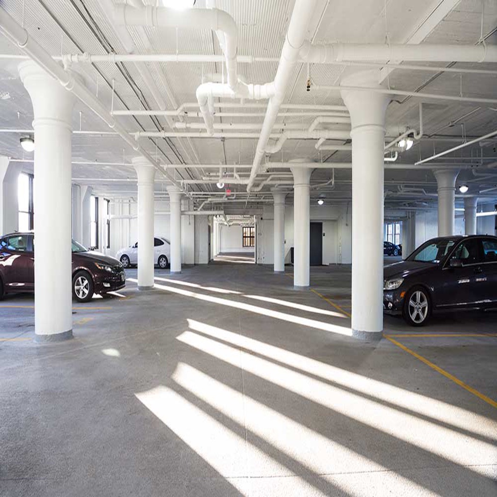
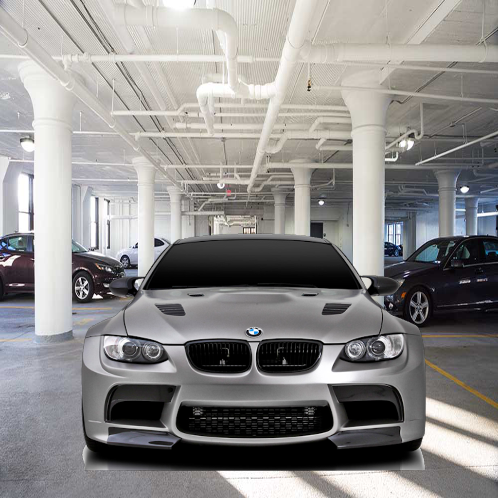
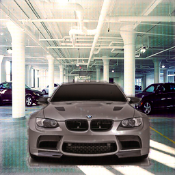
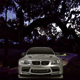
Target Scene	CP	IH [9]	DIPR (ours)

Figure 7: Reshading real cars. Glossy effects in car paint with glitter in them make reshading cars a particularly challenging case with their complex reflective properties. DIPR successfully reshades cars without a distinct shift in object and background color produced by IH. Note the bright patch on the metallic bonnet of the grey car in the top row that may possibly be because of the light source just above it.

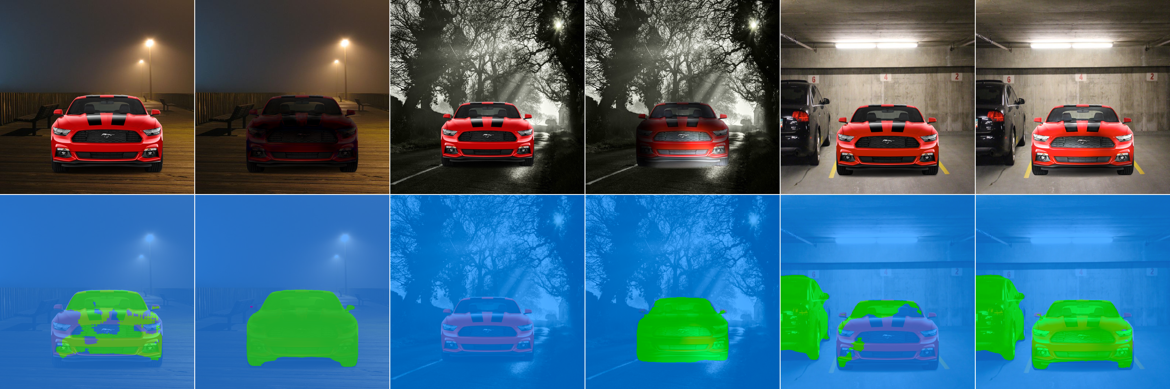
CP

DIPR

CP

DIPR

CP

DIPR

Figure 8: Instance segmentation. DIPR rendered images produce consistent and accurate segmentation maps (bottom row). We observe segmentation fails for cut-and-paste images often. Our key intuition is that the instance segmentation network inherently “knows” if the object’s placement is natural or not and expects the foreground object to have consistent shading with the background. If the object’s shading does not match with that of the background then the resulting segmentation fails to segment object completely.

Consistent Instance Segmentation. We cannot quantitatively evaluate our reshading method when we do not know the ground truth. But we can test whether standard image tasks (which likely benefit from structural consistency in images) perform better on our images. We observe image segmentation methods (we used [8] ) seem to prefer our images (Fig 8) compared to the naïve cut-and-paste. We believe the instance segmentation network inherently “knows” if the object’s placement is natural or not and hence requires the foreground object to be consistent with the background. If not, the segmentation would produce inconsistent results. Our findings are also consistent with Ghiasi et al.[17], who show cut-and-paste is a strong data augmentation method for the instance segmentation. Previous models trained without this augmentation, such as  [8] are sensitive to cut-and-paste images if the inserted fragments contradict the background’s shading. This suggests downstream standard image analysis tasks can serve as a proxy evaluation to further polish reshading methods and also DIPR data augmentations could further improve various recognition tasks.

5 Shape from Shading and its Consistency

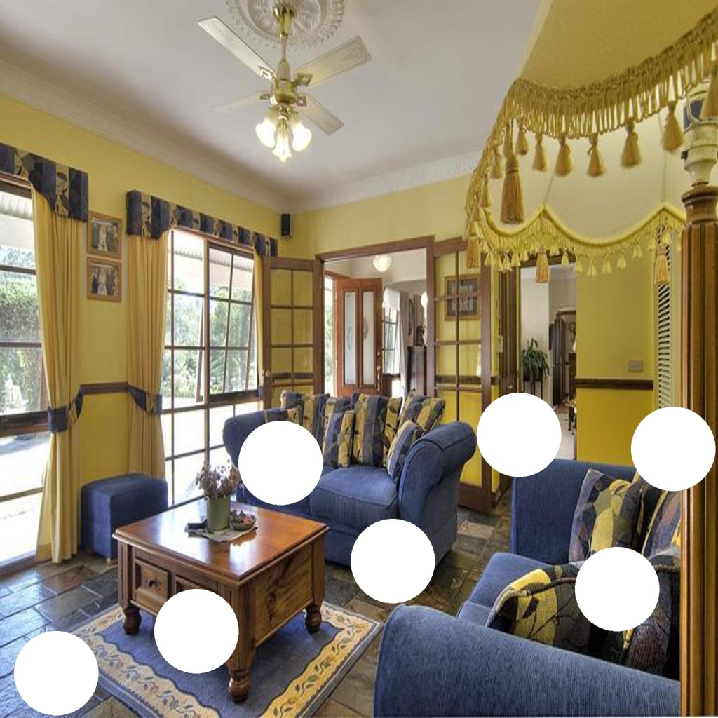
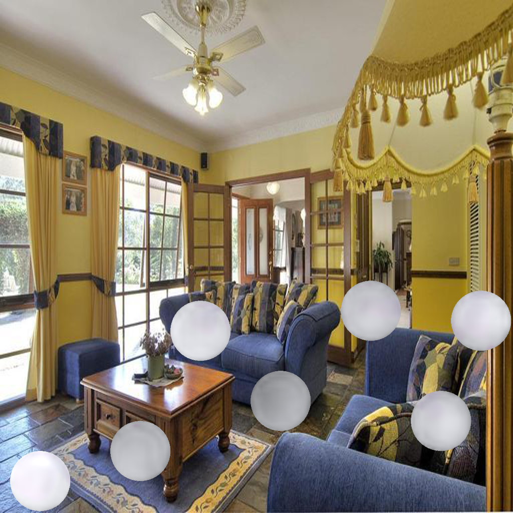
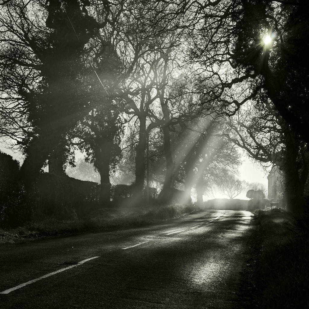
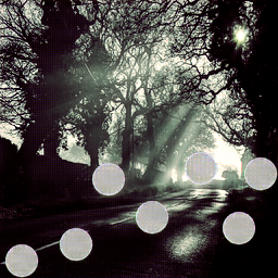
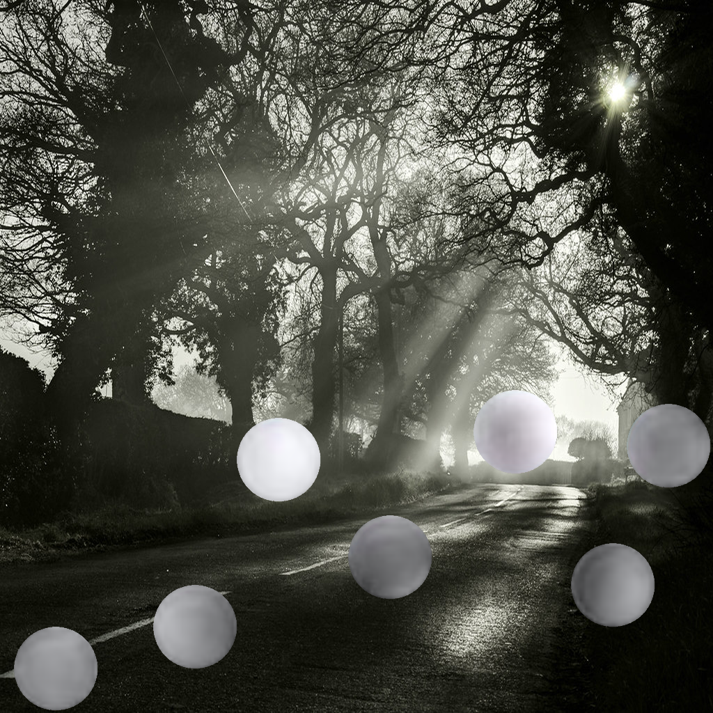
Target Scene	CP	IH [9]	DIPR (ours)

Figure 9: Rendering spheres. DIPR has some implicit notion of the 3D layout of the scene, which is required to choose the appropriate shading. DIPR shades the white discs as spheres (rather better than IH, implying it “knows” about shape; also see Fig. 10).

Reshadings are derived from consistent shapes. DIPR renderings of circles look like spheres (see Fig 9), suggesting the method has some notion of shape. We test if our shadings are consistent, using two procedures: a large scale using singular values and explicit reconstruction (expensive in compute) at a small scale. Results suggest there is indeed some emergent notion of shape, obtained with no shape annotated data.

(a) Large scale: Imagine we have many different reshadings $S_{i,k}$ of a particular inserted shape (we use white circles in albedo). It is known that multiple shadings of the same geometry have important similarities [3]. Assume that the shading value $S_{i,k}({\bf{x}})$ is a slowly changing spatial function of the (unknown) normal ${\bf{N}}({\bf{x}})$, so that $S_{i,k}({\bf{x}})=\sum_{m=1}^{N_{s}}a_{m,k}({\bf{x}})\phi_{m}({\bf{N}}({\bf{x}})$. Assume here that $k$ is small, and $a_{m,k}({\bf{x}})$ are spatially slow. These assumptions apply to, for example, spherical harmonic shading of diffuse surfaces [46]) and shading using the spherical gaussian basis of [29]. Now straighten each image into a vector ${\bf{S}}_{i,k}$. Then these vectors span a $N_{s}$ dimensional space. Form ${\cal D}_{i}=\left[{\bf{S}}_{i,1}^{T},\ldots,{\bf{S}}_{i,N_{o}}\right]$ (where $N_{o}>N_{s}$). We expect the singular values $\sigma_{r}$ of ${\cal M}_{i}$ to be small for $r>N_{s}$ if all the ${\bf{S}}_{i,j}$ are shadings of the same scene, and large if they are not. Using these observations to make a test of consistency requires knowing what is a “small” singular value, and what $N_{s}$ and $N_{o}$ should be. We use $N_{s}=14$ and $200$ sample points on each shading field. We now draw $10000$ sets of $N_{s}$ reshadings from our examples, and look at the test statistic $T{=}\frac{\Pi_{r=10}^{14}\sigma_{r}}{\sigma_{0}^{5}}$. We see a mean of 0.21 and a standard deviation of $7.4{\times}10^{-2}$ for $T$, which appears to be normally distributed. We compare this with a baseline of randomly chosen shading from natural scenes (cropped to the 2D disk). This yields a mean of 0.66 and a standard deviation of $5.9{\times}10^{-2}$. We conclude DIPR reshadings of spheres are strongly different from random shading and display a degree of shape consistency.

(b) Explicit shape reconstruction: We produce explicit shape of our inserted circles from their predicted shadings. We take $7$ reshaded circles, each from two different images. From this pool of $14$, we draw $7$ at random, use them to drive a shape reconstruction procedure (see Appendix; a typical reconstruction in Fig. 10). We then compute the spherical harmonic reshading of the resulting reconstruction that is closest to each of the $7$ held out images and record the mean squared error of the shading residual for each. A small residual means that the shape is consistent across the reshaded circles. Box plots of the resulting residuals for $7$ different splits of the data in Fig. 10. To calibrate, we compare this with $3$ baselines; we reshade: (1) a sphere using actual spherical harmonic shading, reconstruct from reshadings, then predict the held out reshadings (‘SphHarm’), (2) a constant height surface (‘Const’) and (3) a surface reconstructed from smoothed random noise shadings (‘Rand’). These residuals and singular value analysis suggest the reshading network has some form of shape theory as an emergent property.

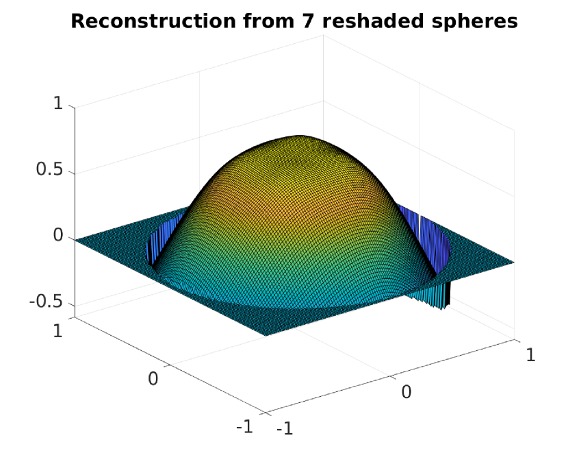
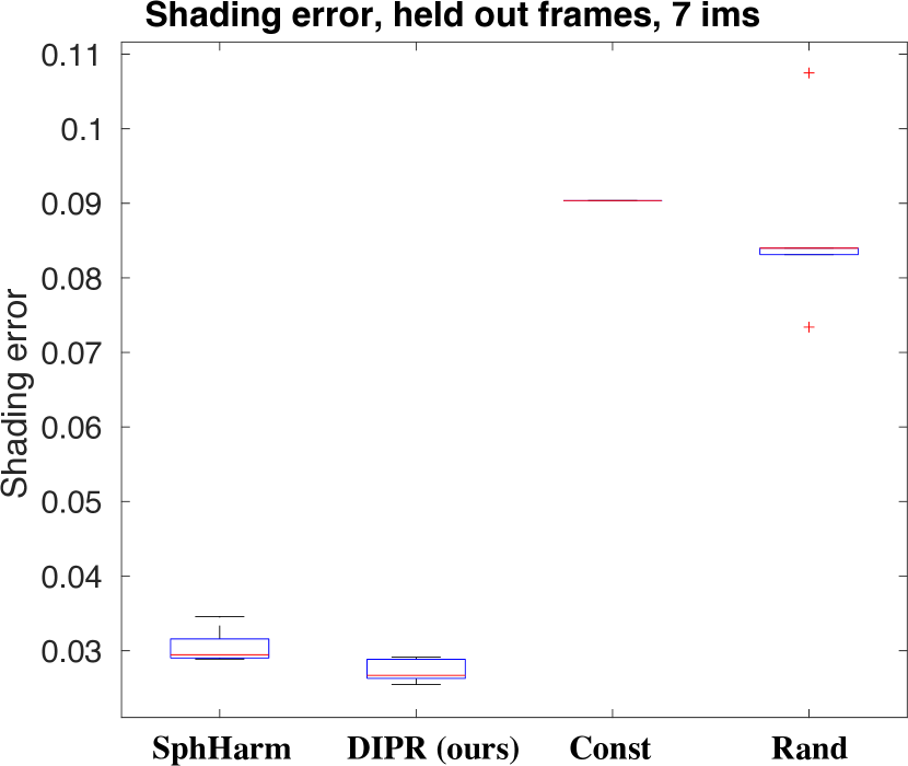
Figure 10: Shape theory and shading consistency: On the left a sample surface reconstruction produced by using $7$ reshaded spheres (Fig. 9). On the right, predicted shading residuals for held out spheres’ shadings using our reconstructed shapes. The residuals suggest: there is a consistent underlying shape. Our DIPR residuals are small. The reconstruction process is reliable but the underlying surface is not quite a sphere. ‘SphHarm’ residuals are also small, but not as small as DIPR. ‘Const’ residuals are large. Therefore, underlying surface is not flat. Smooth ‘Rand’ residuals are large, that is, random shadings cannot explain this consistency.

6 Discussion and Conclusions

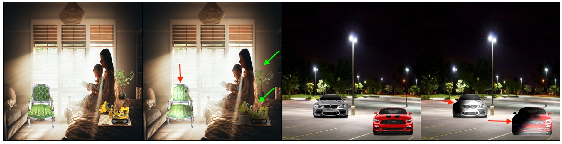
CP

DIPR (ours)

CP

DIPR (ours)

Figure 11: Failure cases. Red arrows point to shading errors. In first image, DIPR aggressively copies background shading onto the chair. However, lego’s and plant’s shading looks plausible. In the second scene, it has two dominant normals – the ground (upwards) and the sky (towards viewer). The lack of third direction results in copying shading either from the sky or the ground.

Limitations. DIPR is slow because DIP takes $15$ mins to render. DIPR cannot cast shadows; very hard and we leave that for our future work. DIPR likely copies shading, so has problems when there is little shading variation and responds poorly when there are “few” normals in the scene (Fig. 11).

Why DIPR works? Corrections to object shading cannot be veridical. [34, 35] finds corrected shading often fool humans more effectively than physically accurate lighting, likely because humans attend to complex materials much more than to consistent lighting [5]. The alternative physics theory [7] argues that the brain employs a set of rules that are convenient, but not strictly physical and a violation leads to perception alarm or affects recognition negatively [16]. Otherwise, the scene “looks right”. This means humans may tolerate a fair degree of error, as long as it is of the right kind. By requiring image to produce consistent inferences, we appear to be forcing errors to be “of the right kind”.

Supplementary Material

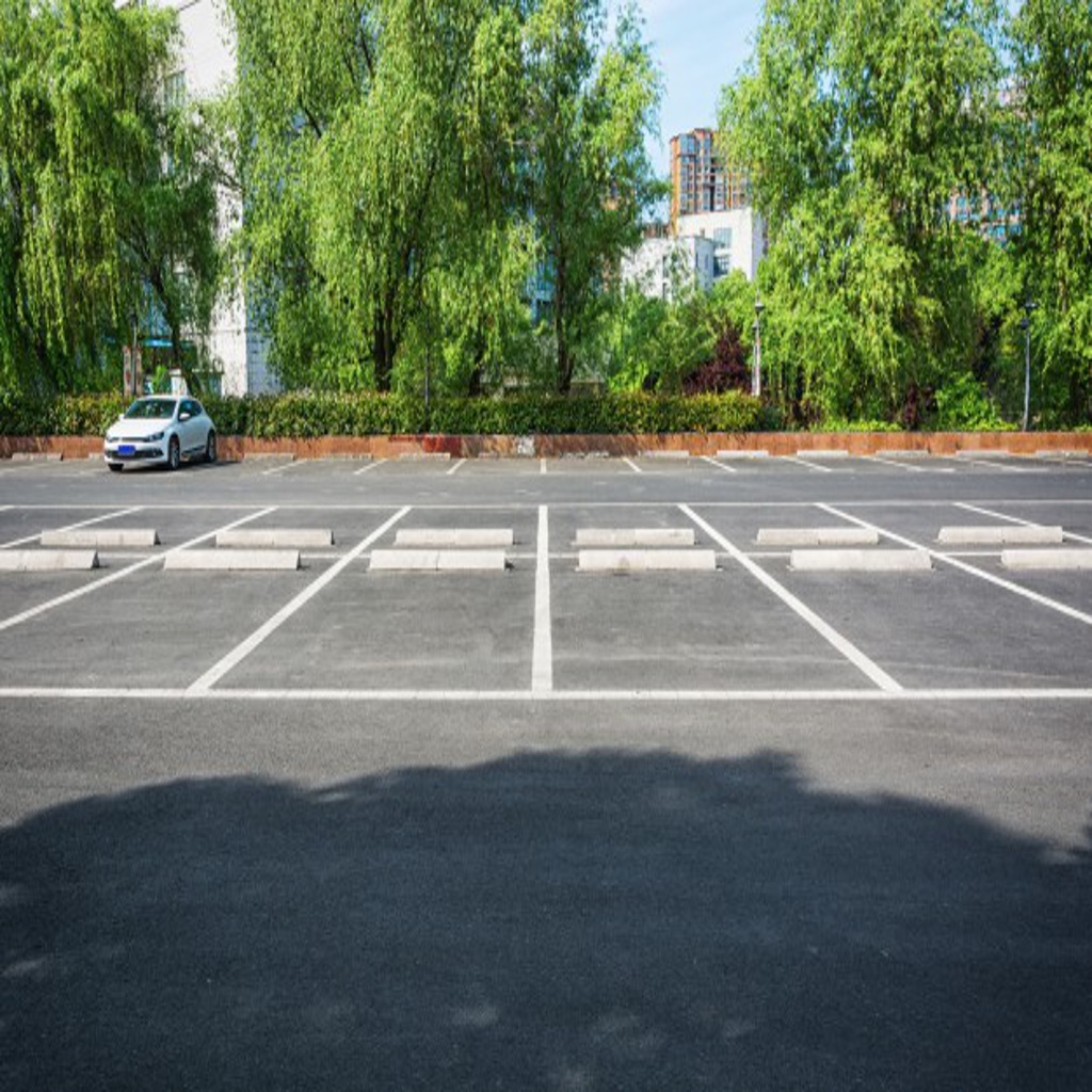
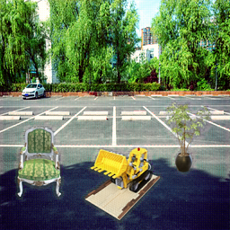
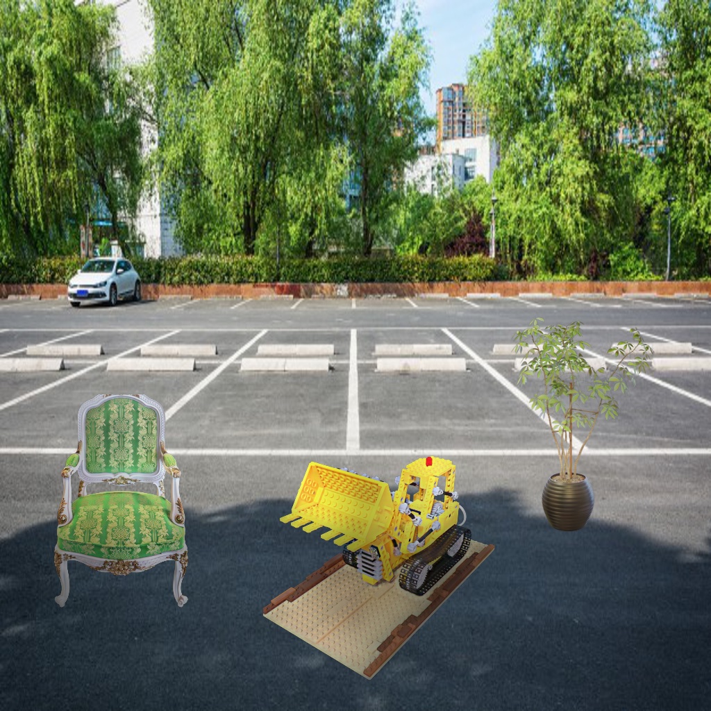
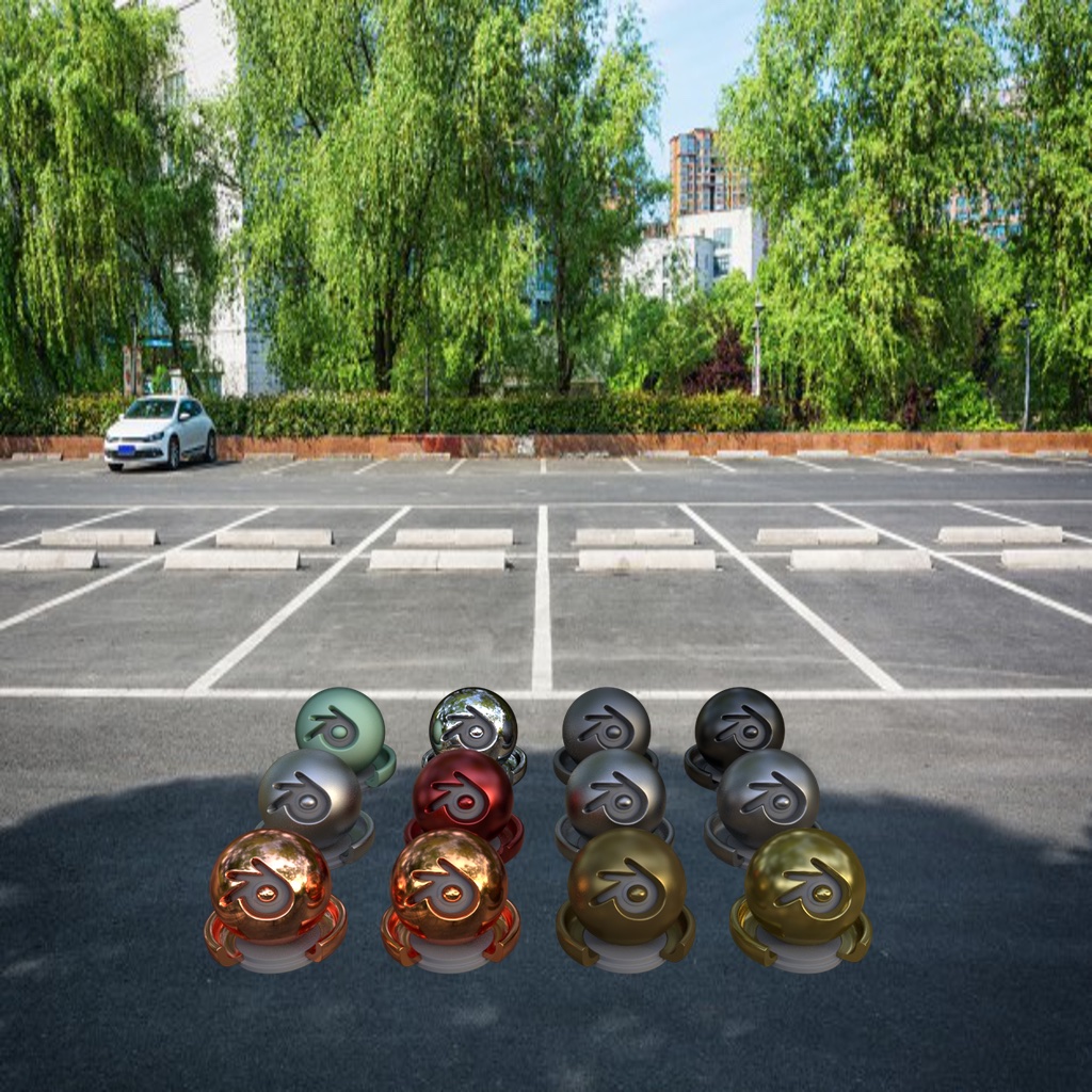
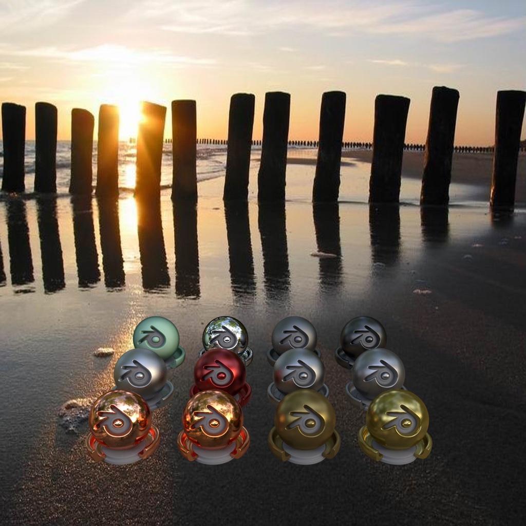
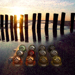
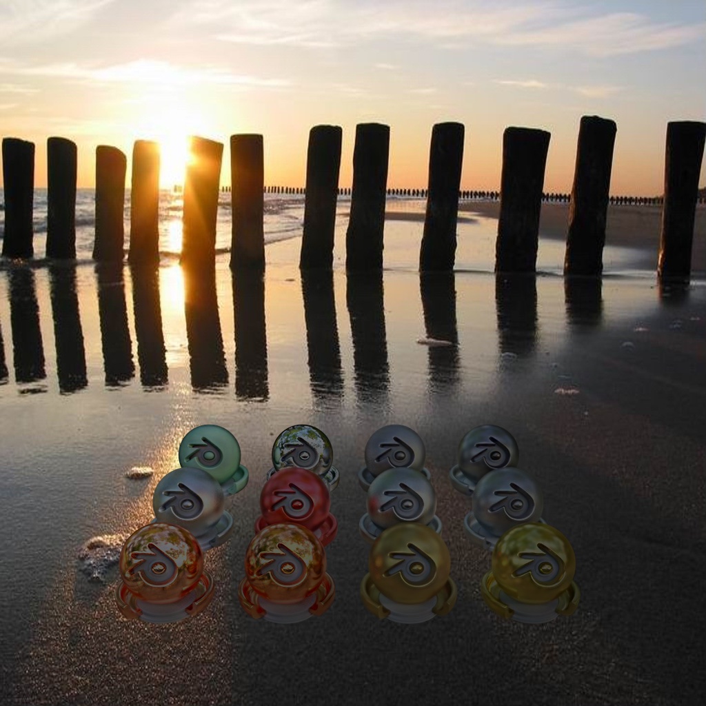
Target Scene	CP	IH [9]	DIPR (ours)

Figure 12: Reshading complex sufaces. DIPR reshades objects with complex surface geometry and complex material properties convincingly, and appears to preserve the identity of the material without a distinct shift in object and background color produced by IH.

Images	NIQE [40]$\downarrow$	CNN-D [55]$\downarrow$	B-T [9]$\uparrow$
IH	38.39	0	0
CP	9.67	0	-0.35
DIPR (ours)	9.78	0	0.04
Target Scene	12.51	0	NA

Table 3: Additional quantitative Analysis for plants, lego, 16-set materials and cars when no ground truth is available. We report numbers for a no-reference image quality estimator (NIQE), a CNN-based tampering detector (CNN-D) and Bradley-Terry (BT) model’s analysis from the user-study. Surprisingly, NIQE is worse for target scenes, CNN-D cannot detect any image as fake, and from the user study between three methods, BT analysis shows our reshaded images are preferred over CP and IH.

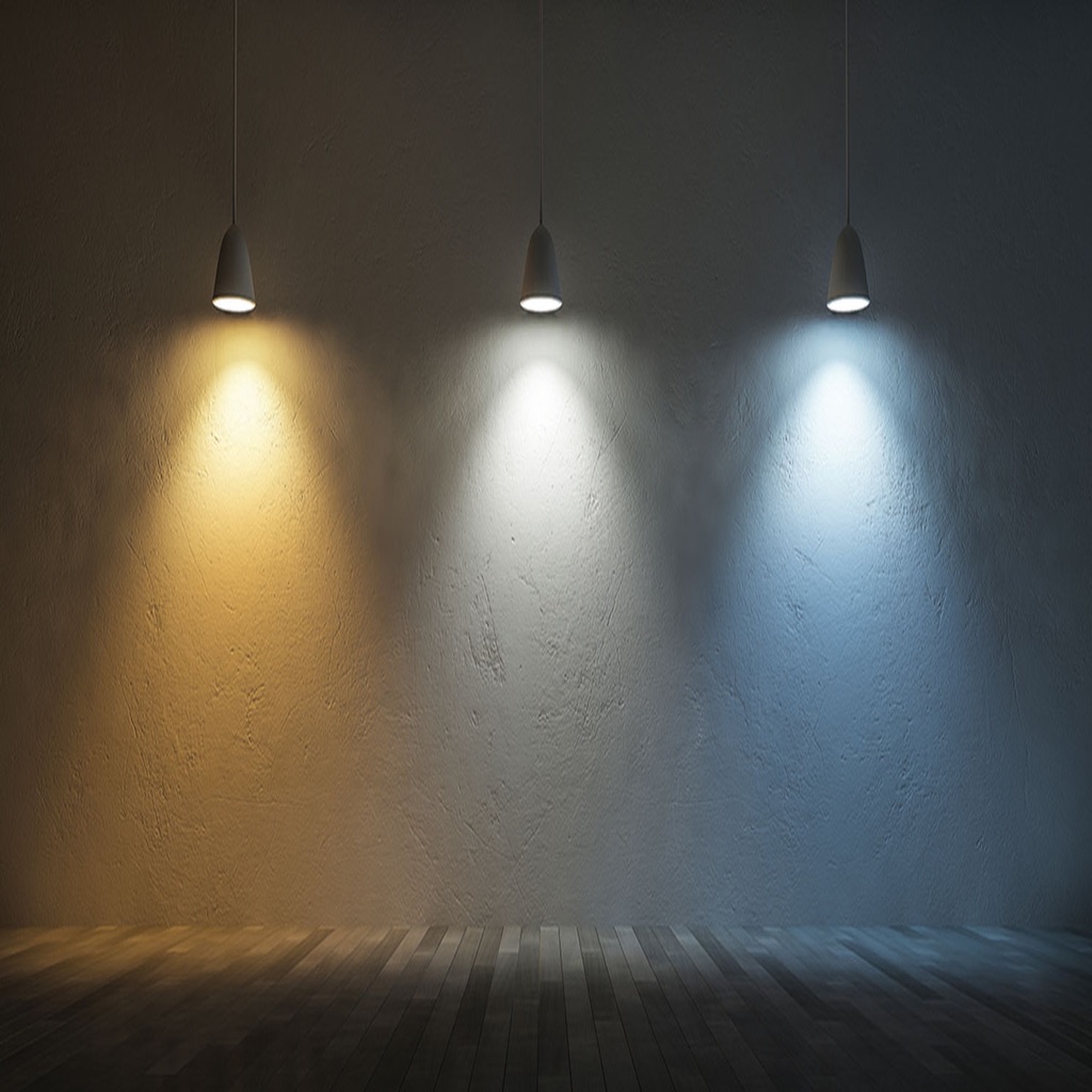
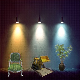
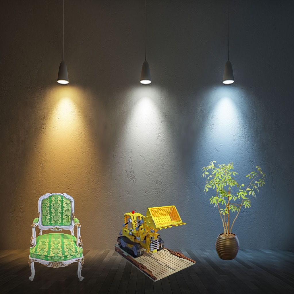
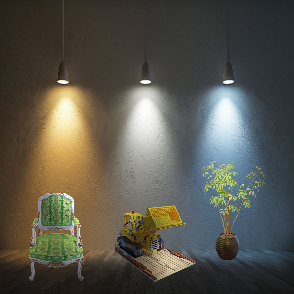
Target Scene	CP	IH [9]	$\mathcal{L}_{recons}+\mathcal{L}_{decomp}$	+$\mathcal{L}_{Z}$	+$\mathcal{L}_{Z}+\mathcal{L}_{Y}$

Figure 13: Ablation Study. We show the role of each of the loss components. Results improve from left to right (see the lego dozer). We find neural shading consistency loss ($\mathcal{L}_{Z}$) helps in improving local changes based on the near-by surroundings and spherical harmonics matching loss ($\mathcal{L}_{Y}$) considers the overall lighting providing complementary solutions. Tab. 2 in the main text has quantitative analysis for losses.

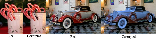
Figure 15: Samples from iharmony dataset [9]. Image Harmonization methods mostly deals with albedo or color correction and for object reshading we expect only shading corrections.

Appendix A 3D Shape Reconstruction

We wish to reconstruct a shape from $N$ images, each showing that shape illuminated by an unknown spherical harmonic illumination field. Illuminants are restricted to the first nine spherical harmonics. We choose $N=7$, because preliminary experiments showed that this was the smallest $N$ that led to reasonably reliable reconstructions. We ignore boundary conditions, and reconstruct by constructing a surface $(x,y,f(x,y))$ and a set of spherical harmonic coefficients $a_{ij}$ to minimize

$$\small\sum_{j=1}^{7}\mid\!\mid\!(\mbox{shading predicted by $f$ and $a_{\cdot j}$}-I_{i})\mid\!\mid\!^{2}\\ +1e-5\mbox{smoothing term}$$ (8)

where the smoothing term is the squared magnitude of the surface gradient. Results described construct a height map on a 128 x 128 grid. We use an approximate Newton method (LBFGS for the Hessian approximation), and use multigrid to accelerate convergence. This reconstruction procedure can be dependent on the start point. We obtain a start point from a random initialization by building a very coarse scale reconstruction (we use 30x30) of a normal field that minimizes shading error, meets boundary conditions (Augmented Lagrangian Method) and is integrable (ALM). We then integrate that normal field to yield a start point.

Appendix B Least Square Formulation for Spherical Harmonics Loss $L_{Y}$

Consider we have $k=m\times n$ pixels in an image, our $\mathcal{N}\in{R}^{k\times 3}$ and $\mathcal{S}\in{R}^{k\times 1}$. We estimate first 9 basis ($\mathcal{B}(\mathcal{N})\in{R}^{k\times 9}$) from $\mathcal{N}$. We can now write $\mathcal{S}=Y\times\mathcal{B}(\mathcal{N})$. The solution for $Y$ is then $\mathcal{B}(\mathcal{N})^{\dagger}\mathcal{S}$. $\mathcal{B}(\mathcal{N})^{\dagger}$ is pseudo-inverse of $\mathcal{B}(\mathcal{N})$.

Appendix C Our Decomposition Model

Our decomposer works as follows. An encoder, with a resnet structure, produces an image code. This is decoded (again with a resnet structure) into an albedo field, a shading field and a gloss field. The albedo field is colored. Shading and gloss field are colorless. The training process accepts albedo, shading and gloss paradigms (generated as samples in advance and cached) and real images from [58]. The real images are given without any of their ground truth. We use them to ensure our image decomposition inferences when recomposed back are able to produce an image that very much looks like real images. We update our decomposer with this residual loss after training with about 50k paradigm samples.

There are four losses. The decomposer must decompose a fake image (constructed out of randomly selected albedo, shading and gloss paradigms) into its correct, known paradigms (mixed L1/L2 loss). The albedo, shading and gloss fields constructed from a real image using our decomposer must combine into that real image (mixed L1/L2 loss). The remaining two losses are adversarial. The albedo field constructed from a real image must fool a classifier trained to distinguish between fake albedo fields and those constructed from real images. Similarly, the shading field constructed from a real image must fool a classifier trained to distinguish between fake shading fields and those constructed from real images.

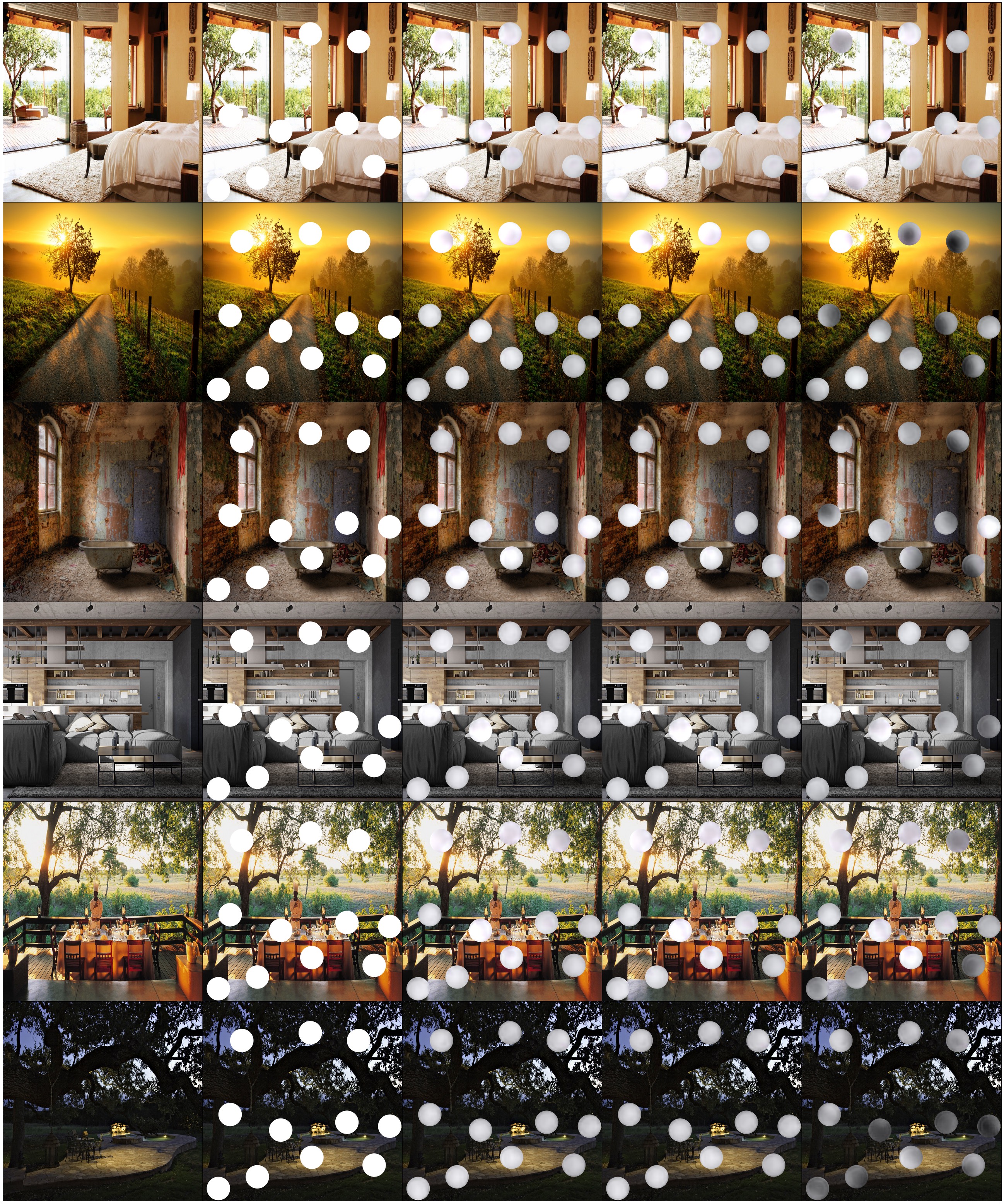
Target  Scene

CP

$\mathcal{L}_{decomp}$

$+\mathcal{L}_{Z}$

$+\mathcal{L}_{Z}+\mathcal{L}_{Y}$

Figure 16: Ablation. We show more renderings of spheres from circle cut-outs (see Fig 10 in main text) in scenes exhibiting complex lighting. Results improve moving from left to right.

Appendix D Post-Processing

Removing DIP artifacts. The input to DIPR are both the target scene and the cut-and-paste image. We let DIP inpaint the shading of the original target image and also the composited image for the masked region. This is analogous to rendering scenes twice with and without inserted object [10, 21]. Doing so means the target scene’s shading field acts like a regularizer that prevents DIP copying cut-and-paste. Furthermore, we can remove DIP (network) specific noisy artifacts. We write ${I}_{obj}$ for the target image rendered by DIP with the object and ${I}_{noobj}$ for the target scene rendered without object, we then form

$${I}_{final}=(1-{M})\odot{I}_{obj}+{M}\odot({I}_{t}+{I}_{obj}-{I}_{noobj})$$ (9)

High-resolution rendering. Our decomposition network can decompose high-resolution intrinsics reliably for real images when trained only on $128$p albedo like intrinsic maps. Since our extrinsic maps are both locally smooth and does not have fine details in them, we can easily upsample them to high-resolution without loss of spatial details. Thus we can render a very high-resolution ($1024$p) composites, without significant loss of geometric detail.

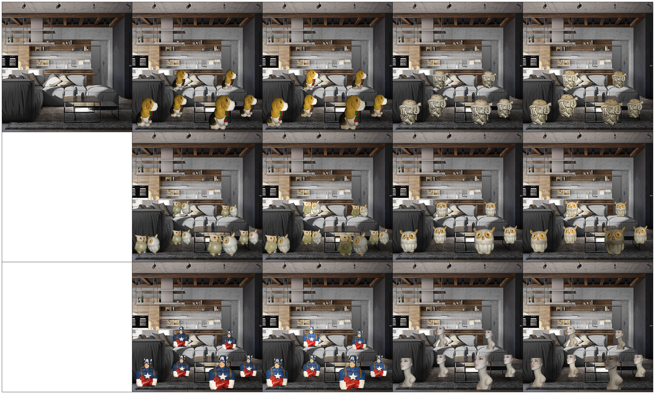
Target  Scene

Cut & Paste

DIPR (Ours)

Cut & Paste

DIPR (Ours)

Figure 17: Multiple Objects. We show multiple objects from [31] added to a scene at different location produce consistent shading that conforms to the target scene’s lighting.

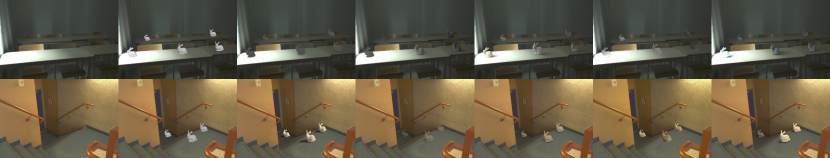
Target Scene

Barron et al. [2]

Gardner et al. [14]

Garon et al. [15]

Li et al. [29]

DIPR (ours)

Simulated GT

Figure 18: Qualitative comparison with SOTA image insertion methods with heavy supervision (which require a geometric and physical model of the inserted objects – the bunnies – and the predicted lighting map for target scene). For the top DIPR image we use Barron’s rendering; for the bottom, we use Gardner’s rendering. DIPR produces plausible shadings in each case, but is outperformed by methods that have access to detailed models of illumination and surface models.

References

- [1] Aayush Bansal, Yaser Sheikh, and Deva Ramanan. Shapes and context: In-the-wild image synthesis & manipulation. In Proceedings of the IEEE Conference on Computer Vision and Pattern Recognition, pages 2317–2326, 2019.
- [2] Jonathan T Barron and Jitendra Malik. Shape, illumination, and reflectance from shading. IEEE transactions on pattern analysis and machine intelligence, 2014.
- [3] Peter N Belhumeur and David J Kriegman. What is the set of images of an object under all possible illumination conditions? International Journal of Computer Vision, 1998.
- [4] Sean Bell, Kavita Bala, and Noah Snavely. Intrinsic images in the wild. ACM Transactions on Graphics (TOG), 2014.
- [5] Julia Berzhanskaya, Gurumurthy Swaminathan, Jacob Beck, and Ennio Mingolla. Remote effects of highlights on gloss perception. Perception, 2005.
- [6] Sai Bi, Xiaoguang Han, and Yizhou Yu. An l 1 image transform for edge-preserving smoothing and scene-level intrinsic decomposition. ACM Transactions on Graphics (TOG), 2015.
- [7] Patrick Cavanagh and George A Alvarez. Tracking multiple targets with multifocal attention. Trends in cognitive sciences, 9(7):349–354, 2005.
- [8] Liang-Chieh Chen, George Papandreou, Florian Schroff, and Hartwig Adam. Rethinking atrous convolution for semantic image segmentation. arXiv preprint arXiv:1706.05587, 2017.
- [9] Wenyan Cong, Jianfu Zhang, Li Niu, Liu Liu, Zhixin Ling, Weiyuan Li, and Liqing Zhang. Dovenet: Deep image harmonization via domain verification. In Proceedings of the IEEE/CVF Conference on Computer Vision and Pattern Recognition, pages 8394–8403, 2020.
- [10] Paul Debevec. Rendering synthetic objects into real scenes: bridging traditional and image-based graphics with global illumination and high dynamic range photography. In Proceedings of the 25th annual conference on Computer graphics and interactive techniques, 1998.
- [11] Debidatta Dwibedi, Ishan Misra, and Martial Hebert. Cut, paste and learn: Surprisingly easy synthesis for instance detection. In Proceedings of the IEEE International Conference on Computer Vision, pages 1301–1310, 2017.
- [12] Qingnan Fan, Jiaolong Yang, Gang Hua, Baoquan Chen, and David Wipf. Revisiting deep intrinsic image decompositions. In Proceedings of the IEEE conference on computer vision and pattern recognition, 2018.
- [13] DA Forsyth and Jason J Rock. Intrinsic image decomposition using paradigms. arXiv preprint arXiv:2011.10512, 2020.
- [14] Marc-André Gardner, Yannick Hold-Geoffroy, Kalyan Sunkavalli, Christian Gagné, and Jean-François Lalonde. Deep parametric indoor lighting estimation. In Proceedings of the IEEE International Conference on Computer Vision, 2019.
- [15] Mathieu Garon, Kalyan Sunkavalli, Sunil Hadap, Nathan Carr, and Jean-François Lalonde. Fast spatially-varying indoor lighting estimation. In Proceedings of the IEEE Conference on Computer Vision and Pattern Recognition, 2019.
- [16] Isabel Gauthier, Pepper Williams, Michael J Tarr, and James Tanaka. Training ‘greeble’experts: a framework for studying expert object recognition processes. Vision research, 38(15-16):2401–2428, 1998.
- [17] Golnaz Ghiasi, Yin Cui, Aravind Srinivas, Rui Qian, Tsung-Yi Lin, Ekin D Cubuk, Quoc V Le, and Barret Zoph. Simple copy-paste is a strong data augmentation method for instance segmentation. arXiv preprint arXiv:2012.07177, 2020.
- [18] Zonghui Guo, Dongsheng Guo, Haiyong Zheng, Zhaorui Gu, Bing Zheng, and Junyu Dong. Image harmonization with transformer. In Proceedings of the IEEE/CVF International Conference on Computer Vision, pages 14870–14879, 2021.
- [19] Yannick Hold-Geoffroy, Akshaya Athawale, and Jean-François Lalonde. Deep sky modeling for single image outdoor lighting estimation. In Proceedings of the IEEE Conference on Computer Vision and Pattern Recognition, 2019.
- [20] Jiaya Jia, Jian Sun, Chi-Keung Tang, and Heung-Yeung Shum. Drag-and-drop pasting. ACM Transactions on graphics (TOG), 25(3):631–637, 2006.
- [21] Kevin Karsch, Varsha Hedau, David Forsyth, and Derek Hoiem. Rendering synthetic objects into legacy photographs. ACM Transactions on Graphics (TOG), 2011.
- [22] Kevin Karsch, Kalyan Sunkavalli, Sunil Hadap, Nathan Carr, Hailin Jin, Rafael Fonte, Michael Sittig, and David Forsyth. Automatic scene inference for 3d object compositing. ACM Transactions on Graphics (TOG), 2014.
- [23] Jean-François Lalonde, Derek Hoiem, Alexei A Efros, Carsten Rother, John Winn, and Antonio Criminisi. Photo clip art. ACM transactions on graphics (TOG), 2007.
- [24] Edwin H Land. Color vision and the natural image. part i. Proceedings of the National Academy of Sciences of the United States of America, 1959.
- [25] Edwin H Land. Color vision and the natural image part ii. Proceedings of the National Academy of Sciences of the United States of America, 1959.
- [26] Edwin H Land. The retinex theory of color vision. Scientific american, 1977.
- [27] Edwin H Land and John J McCann. Lightness and retinex theory. Josa, 1971.
- [28] Donghoon Lee, Sifei Liu, Jinwei Gu, Ming Yu Liu, Ming Hsuan Yang, and Jan Kautz. Context-aware synthesis and placement of object instances. In Advances in Neural Information Processing Systems, 2018.
- [29] Zhengqin Li, Mohammad Shafiei, Ravi Ramamoorthi, Kalyan Sunkavalli, and Manmohan Chandraker. Inverse rendering for complex indoor scenes: Shape, spatially-varying lighting and svbrdf from a single image. In Proceedings of the IEEE Conference on Computer Vision and Pattern Recognition, 2020.
- [30] Zhengqi Li and Noah Snavely. Cgintrinsics: Better intrinsic image decomposition through physically-based rendering. In Proceedings of the European Conference on Computer Vision (ECCV), 2018.
- [31] Zhengqi Li and Noah Snavely. Learning intrinsic image decomposition from watching the world. In Proceedings of the IEEE Conference on Computer Vision and Pattern Recognition, 2018.
- [32] Zhengqin Li, Zexiang Xu, Ravi Ramamoorthi, Kalyan Sunkavalli, and Manmohan Chandraker. Learning to reconstruct shape and spatially-varying reflectance from a single image. ACM Transactions on Graphics (TOG), 2018.
- [33] Zicheng Liao, Ali Farhadi, Yang Wang, Ian Endres, and David Forsyth. Building a dictionary of image fragments. In 2012 IEEE Conference on Computer Vision and Pattern Recognition, pages 3442–3449. IEEE, 2012.
- [34] Zicheng Liao, Kevin Karsch, and David Forsyth. An approximate shading model for object relighting. In Proceedings of the IEEE Conference on Computer Vision and Pattern Recognition, 2015.
- [35] Zicheng Liao, Kevin Karsch, Hongyi Zhang, and David Forsyth. An approximate shading model with detail decomposition for object relighting. International Journal of Computer Vision, 2019.
- [36] Tsung-Yi Lin, Michael Maire, Serge Belongie, James Hays, Pietro Perona, Deva Ramanan, Piotr Dollár, and C Lawrence Zitnick. Microsoft coco: Common objects in context. In European conference on computer vision. Springer, 2014.
- [37] Jun Ling, Han Xue, Li Song, Rong Xie, and Xiao Gu. Region-aware adaptive instance normalization for image harmonization. In Proceedings of the IEEE/CVF Conference on Computer Vision and Pattern Recognition, 2021.
- [38] Guilin Liu, Fitsum A Reda, Kevin J Shih, Ting-Chun Wang, Andrew Tao, and Bryan Catanzaro. Image inpainting for irregular holes using partial convolutions. In Proceedings of the European Conference on Computer Vision (ECCV), 2018.
- [39] Ben Mildenhall, Pratul P Srinivasan, Matthew Tancik, Jonathan T Barron, Ravi Ramamoorthi, and Ren Ng. Nerf: Representing scenes as neural radiance fields for view synthesis. arXiv preprint arXiv:2003.08934, 2020.
- [40] Anish Mittal, Rajiv Soundararajan, and Alan C Bovik. Making a “completely blind” image quality analyzer. IEEE Signal processing letters, 20(3):209–212, 2012.
- [41] Vladimir Nekrasov, Thanuja Dharmasiri, Andrew Spek, Tom Drummond, Chunhua Shen, and Ian Reid. Real-time joint semantic segmentation and depth estimation using asymmetric annotations. In 2019 International Conference on Robotics and Automation (ICRA). IEEE, 2019.
- [42] Thomas Nestmeyer, Jean-François Lalonde, Iain Matthews, Epic Games, Andreas Lehrmann, and AI Borealis. Learning physics-guided face relighting under directional light. 2020.
- [43] Patrick Pérez, Michel Gangnet, and Andrew Blake. Poisson image editing. In ACM SIGGRAPH 2003 Papers, pages 313–318, 2003.
- [44] Ken Perlin. An image synthesizer. ACM Siggraph Computer Graphics, 1985.
- [45] Vilayanur S Ramachandran. Perceiving shape from shading. Scientific American, 1988.
- [46] Ravi Ramamoorthi and Pat Hanrahan. On the relationship between radiance and irradiance: determining the illumination from images of a convex lambertian object. JOSA A, 2001.
- [47] Edgar Schönfeld, Bernt Schiele, and Anna Khoreva. A u-net based discriminator for generative adversarial networks. arXiv preprint arXiv:2002.12655, 2020.
- [48] Meng-Li Shih, Shih-Yang Su, Johannes Kopf, and Jia-Bin Huang. 3d photography using context-aware layered depth inpainting. In Proceedings of the IEEE/CVF Conference on Computer Vision and Pattern Recognition, pages 8028–8038, 2020.
- [49] Shuran Song and Thomas Funkhouser. Neural illumination: Lighting prediction for indoor environments. In Proceedings of the IEEE Conference on Computer Vision and Pattern Recognition, 2019.
- [50] Pratul P Srinivasan, Ben Mildenhall, Matthew Tancik, Jonathan T Barron, Richard Tucker, and Noah Snavely. Lighthouse: Predicting lighting volumes for spatially-coherent illumination. In Proceedings of the IEEE Conference on Computer Vision and Pattern Recognition, 2020.
- [51] Tiancheng Sun, Jonathan T Barron, Yun-Ta Tsai, Zexiang Xu, Xueming Yu, Graham Fyffe, Christoph Rhemann, Jay Busch, Paul Debevec, and Ravi Ramamoorthi. Single image portrait relighting. ACM Transactions on Graphics (Proceedings SIGGRAPH), 2019.
- [52] Kalyan Sunkavalli, Micah K Johnson, Wojciech Matusik, and Hanspeter Pfister. Multi-scale image harmonization. ACM Transactions on Graphics (TOG), 29(4):1–10, 2010.
- [53] Yi-Hsuan Tsai, Xiaohui Shen, Zhe Lin, Kalyan Sunkavalli, Xin Lu, and Ming-Hsuan Yang. Deep image harmonization. In Proceedings of the IEEE Conference on Computer Vision and Pattern Recognition, pages 3789–3797, 2017.
- [54] Dmitry Ulyanov, Andrea Vedaldi, and Victor Lempitsky. Deep image prior. In Proceedings of the IEEE Conference on Computer Vision and Pattern Recognition, 2018.
- [55] Sheng-Yu Wang, Oliver Wang, Richard Zhang, Andrew Owens, and Alexei A Efros. Cnn-generated images are surprisingly easy to spot…for now. In CVPR, 2020.
- [56] Ye Yu and William AP Smith. Inverserendernet: Learning single image inverse rendering. In Proceedings of the IEEE Conference on Computer Vision and Pattern Recognition, 2019.
- [57] Richard Zhang, Phillip Isola, Alexei A Efros, Eli Shechtman, and Oliver Wang. The unreasonable effectiveness of deep features as a perceptual metric. In CVPR, 2018.
- [58] Bolei Zhou, Hang Zhao, Xavier Puig, Sanja Fidler, Adela Barriuso, and Antonio Torralba. Scene parsing through ade20k dataset. In Proceedings of the IEEE conference on computer vision and pattern recognition, 2017.
- [59] Hao Zhou, Sunil Hadap, Kalyan Sunkavalli, and David W Jacobs. Deep single-image portrait relighting. In Proceedings of the IEEE International Conference on Computer Vision, 2019.